Simulation of Electromagnetic Forming Process and Optimization of Geometric Parameters of Perforated Al Sheet Using RSM

Abstract

Electromagnetic forming (EMF) is a kind of high-speed forming technology that can be useful for materials like aluminum. EMF helps to overcome the limitations of traditional forming. Due to this ability, the use of EMF in automotive applications has risen in recent years. The application of finite element software packages such as ANSYS 22 gives numerical modelling capabilities to simulate the EMF process and to design the forming process. Hence, the aim of this research work is to build and study the three-dimensional finite element model for the electromagnetic forming process and analyze the geometric parameters influencing the deformation of the perforated sheet with a design of experiments (DOE) approach. The finite element simulation is used in two stages. In the first stage, the electromagnetic force or Lorentz force striking the workpiece (i.e., Al sheet) is predicted using the ANSYS 22 Emag module. In the second stage, the predicted Lorentz force is then applied on an Al sheet to calculate the sheet deformation. The deformation of the sheet is predicted for different combinations of the geometric parameters of the sheet, such as open area percentage, ligament ratio (LR) and size of the hole, using ANSYS 22 Structural. In the DOE, response surface methodology (RSM) is used by considering the geometric parameters of perforated sheet such as open area percentage, ligament ratio (LR) and size of the hole. To minimize the number of experiments, an RSM model named central composite design (CCD) is employed. Further, the optimization study finds that the maximum deformation 0.0435 mm is calculated for the optimized combination of 25% open area, 0.14 LR and 4 mm hole size.

1. Introduction

In the electromagnetic forming (EMF) process, metal sheets are deformed by using repulsive force created between the opposite magnetic fields in adjacent conductors. When a pulsed current passes through the coil, it generates transient magnetic field which in turn induces eddy currents in the metallic workpiece opposite to the direction of the current passing through the coil. Due to the induced eddy current, a repulsive force is generated between the work piece and the forming coil, which causes the deformation of the workpiece.

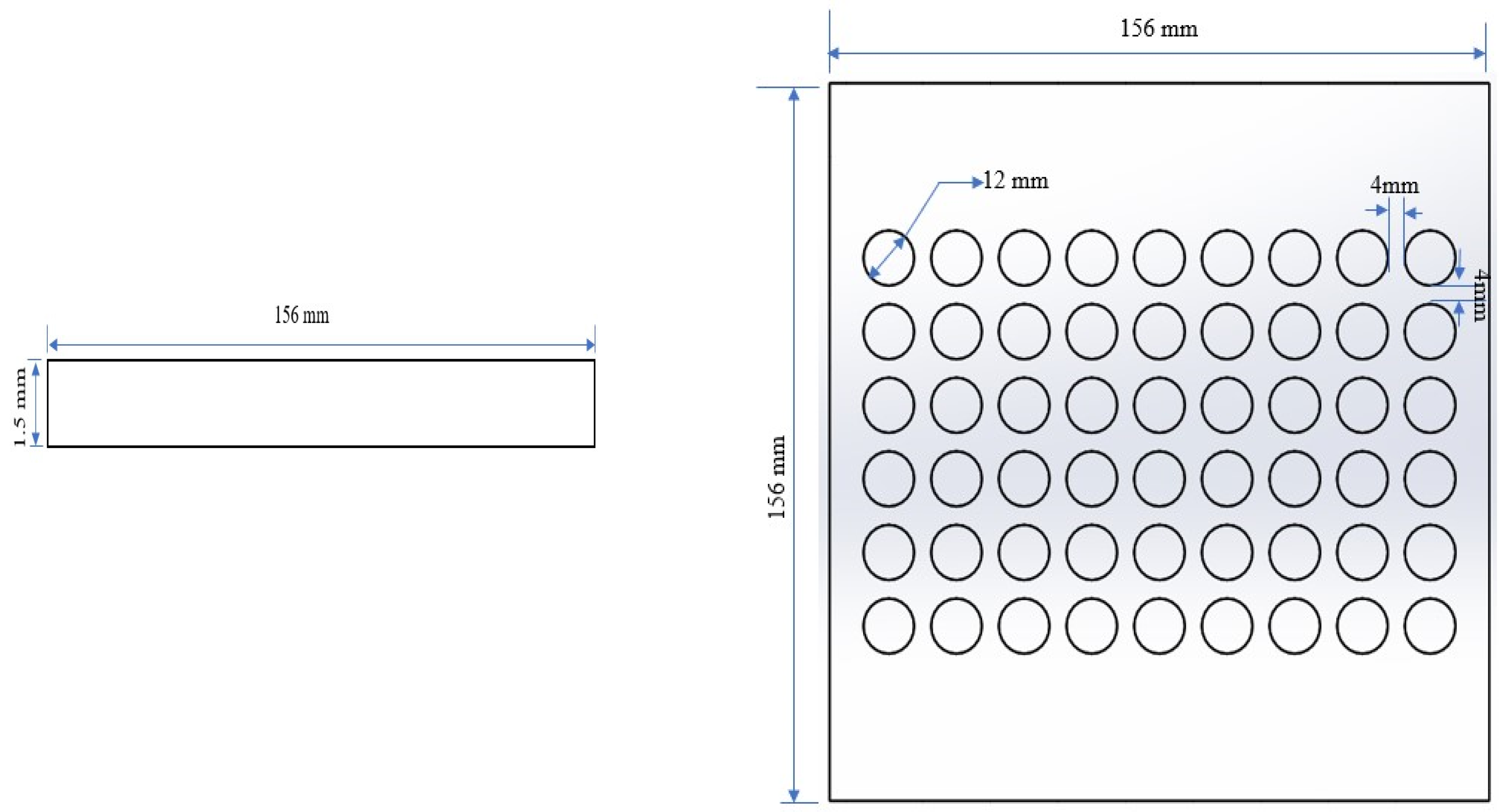
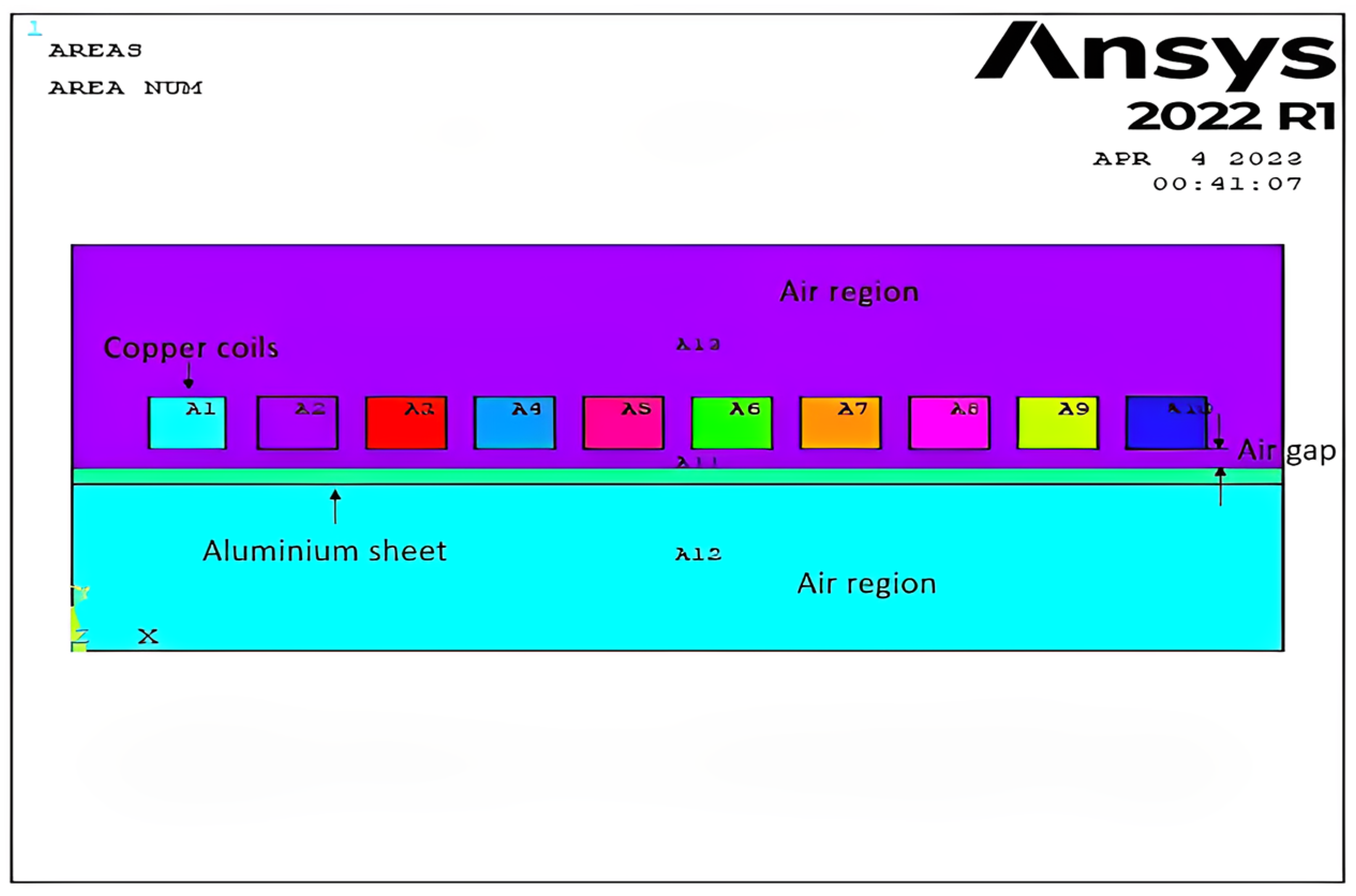
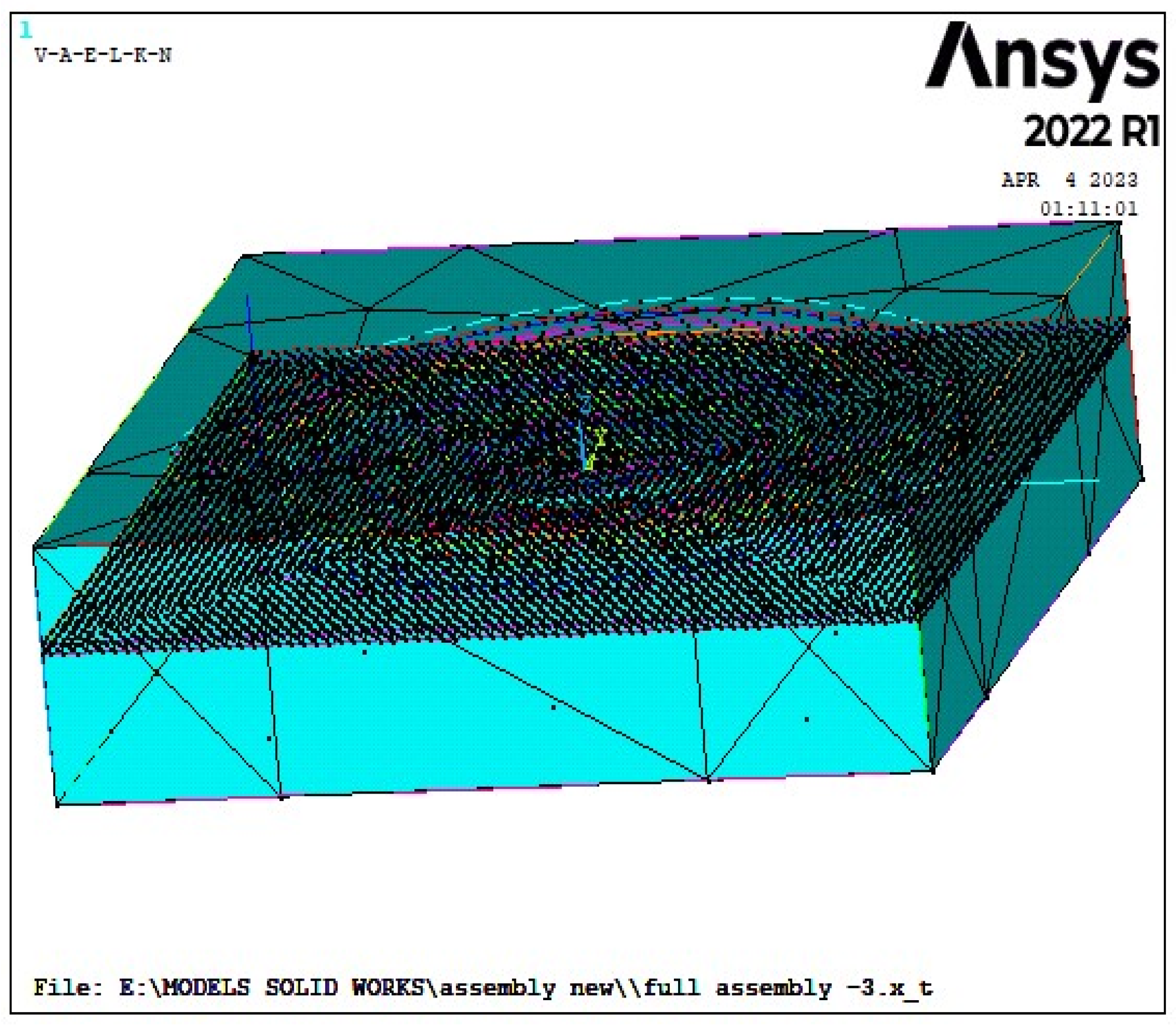
This repulsive force causes the workpiece to stress beyond its yield limit, so that the workpiece is shaped permanently at high strain rates. In order to design an EMF system successfully and analyze its performance, appropriate numerical methods must be used in order to have cost effective industrial applications. For calculating the magnetic forces, a three-dimensional (3D) finite element model is created. To determine the deformation, this generated magnetic force is applied to a perforated aluminum 5052 sheet.

1.1. Working Principle of EMF

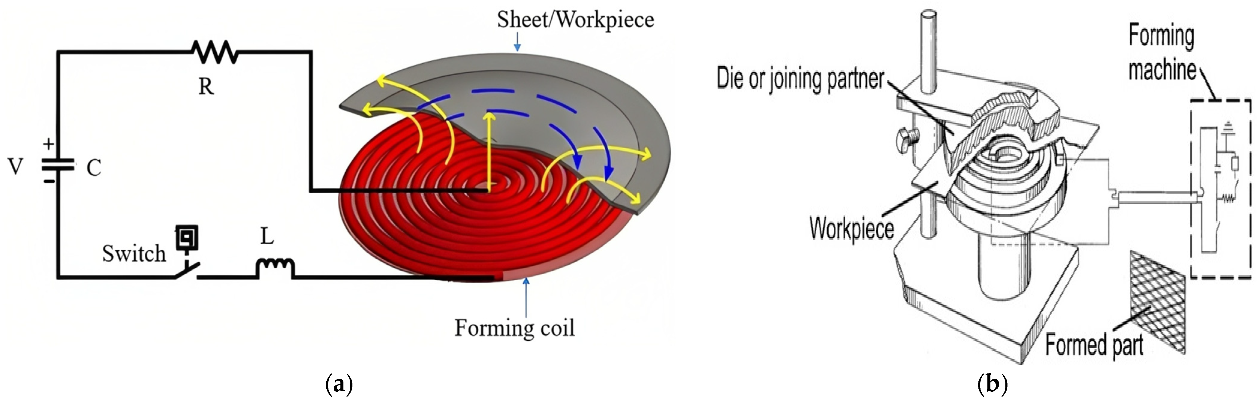
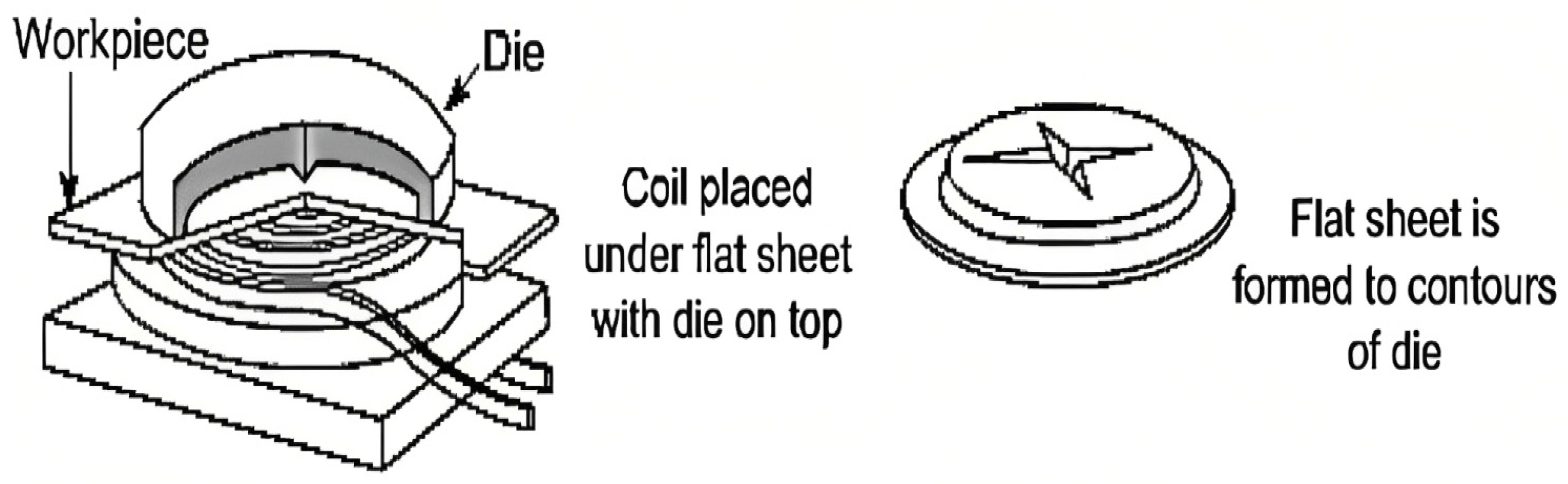
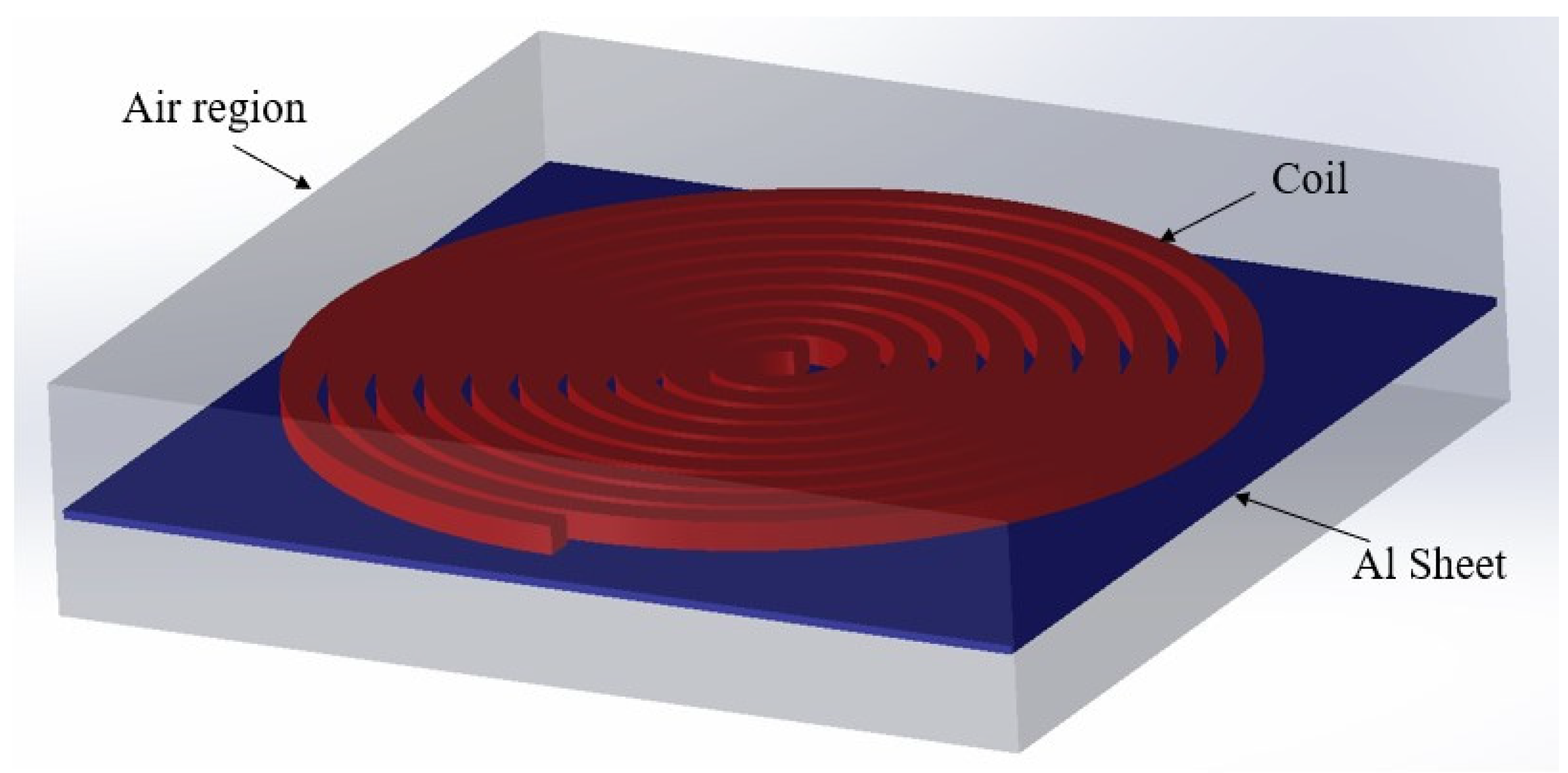
In electromagnetic forming, Lorentz forces (magnetic forces) are used to deform metallic sheets at high speeds. Figure 1a,b shows the set-up of the EMF process, consisting of a low inductance electrical circuit with large capacitance, which supplies electric current through a (forming) coil tool. Therefore, by Faraday’s law of induction, the current induces a magnetic flux in the nearby conductor (workpiece), which generates eddy current. This eddy current induces magnetic forces, causing the deformation of the metal sheet (workpiece) beyond its elastic limit. The impulse electromagnetic system is used for different applications, including welding, compression or expansion of sheet metal tubes, and the forming of flat metal sheets (e.g., Figure 2) such as panels used in the automotive industry. The arrangement of an impulse electromagnetic forming system depends on the geometries of the forming coils and the geometry of the workpiece to be modified.

The fundamental equations representing the electromagnetic fields are governed by Maxwell, as given in Equations (1)–(5) [1].

$$\Delta \times \overline{E}=-\frac{d\overline{B}}{\mathrm{dt}}$$

(1)

$$\Delta \times \overline{H} = \overline{J}$$

(2)

$$\Delta ·\overline{B} = 0$$

(3)

$$\overline{B} = \mathsf{\mu }\overline{H}$$

(4)

$$\Delta ·\overline{J} = 0$$

(5)

where, $\overline{E}$ is the electric field, $\overline{H}$ is the magnetic field intensity, $\overline{B}$ is the magnetic field density, μ is the permeability, $\overline{F}$ is the Lorentz force, and $\overline{J}$ is the current density.

The current density dependence can be represented per Equation (6):

$$\overline{J} = \mathsf{\sigma }\overline{E},$$

(6)

in which σ is the electrical conductivity of workpiece.

In 1895, Lorentz stated that the force density ($\overline{F}$) acting on the workpiece depends upon the magnetic flux density ($\overline{B}$), generated due to the supplied current density ($\overline{J}$), given as:

$$\overline{F} = \overline{J} \times \overline{B}$$

(7)

1.2. Existing Research Efforts

Furth and Waniek [2] first introduced the electromagnetic forming by which the workpiece is pushed away from the tool coil. The authors suggested using two different coils to establish pulling forces, which in turn allow the formation of bulges on hollow workpieces or large sheets.

Kleiner et al. [3] analyzed the effects of process parameters such as strain rate and magnetic pressure on workpiece deformation for tubular as well as flat sheet workpieces. Meriched et al.’s [4] investigation developed a numerical technique to solve the three coupled problems: electric circuit analysis, electromagnetic force and the deformation of a circular thin sheet using a flat spiral coil. Fenton et al. [5] used a computer code ALE (Arbitrary Lagrangian–Eulerian) to simulate the EMF process. They validated the simulation results of deformation of a thin aluminum sheet using two dimensional axi-symmetric models with experimental results. Zhang et al. [6] simulated a 2D axi-symmetric model in the COMSOL Multiphysics software package, and analyzed the dynamic behavior of a sheet metal workpiece. Reese et al. [7] focused on the use of coarse mesh, with which the accuracy of the numerical solution can be increased. It also reduced the computational time by reducing the gauss points. This reduced integration and hourglass stabilization method may be used to couple the mechanical and electromagnetic fields more efficiently. Mamalis et al. [8] used the ANSYS finite element code and LS-DYNA software to model a 2D axi-symmetric aluminum alloy sheet using a loose coupling approach. The authors also validated the current numerical model with experimental results using an equivalent circuit method.

Another 2D finite element model was developed by Luca [9], using FLUX2D software. The stresses and strains on the AlMn0.5Mg0.5 sheet are calculated using the ALGOR software. These numerical simulation results were compared with the EMF experiment and found to be in good agreement with each other.

Siddiqui et al. [10] considered the simulation of the electromagnetic forming process as two separate problems, i.e., an electromagnetic problem and a mechanical problem. The magnetic forces were predicted with the help of a finite element code named FEMM4.0. These forces were taken as the input boundary condition, and by a subroutine VDLOAD, were then applied to a finite element model with commercial FE software ABAQUS/Explicit. Unger et al. [11] investigated the coupled multi-field formulation of the electromagnetic forming process with which a thermo-magneto-mechanical model was developed, and simulation was performed on an aluminum alloy (AA 6005) plate. Denga et al. [12] studied electromagnetic attractive force forming, in which ANSYS software was used to simulate a 2D axisymmetric model. Along the flat coil, magnetic flux was distributed and validated with the experiment results, indicating that the workpiece was attracted to the coil and moved quickly.

Khandelwal et al. [13] performed experimental and numerical analyses of EMF on aluminum tubes. They considered discharge energy, standoff distance (gap between workpiece and coil) and workpiece thickness as influencing parameters on the workpiece’s deformation using an ANOVA approach. Imbert et al. [14] employed a commercial FEA package LS-DYNA to carry out numerical simulation of EMF process on conical and V-shaped AA 5754 sheets. For both models, the numerical and experimental results were compared and found to be in good agreement. The authors concluded that the formability of the sheets was improved due to the reduction in tool–sheet interaction. To explore the numerical approaches to the EMF process, Parez et al. [15] used software such as Maxwell 3D, Sysmagna^® and Pam-Stamp2G. These pieces of software were used to model sequential coupling and loose coupling, and their results were validated with experimental results carried out on an Al 1050 sheet.

Siddiqui et al. [16] carried out numerical simulation of an Al 1050 aluminum tube, with the help of FE code FORTRAN and FEA software FEMM. The results were compared with experimental results from earlier literature. Then, these numerical results were introduced in FEA software ABAQUS/Explicit to predict the electromagnetic tube expansion process. Bahmani et al. [17] used field shapers to concentrate the magnetic field at required points of metal sheet. They concluded that in 3D modeling of the EMF process, the magnitude of magnetic flux density generated is greater than 2D axisymmetric simulation by 15%. Haiping et al. [18] formulated a sequential coupling approach to model a 2D axisymmetric electromagnetic model in ANSYS for the process of electromagnetic tube compression. They analyzed the effect of tube deformation on electromagnetic geometry so that accuracy of simulation would be improved.

Xu et al. [19] focused on using various meshing types in the simulation of the EMF process in order to reduce the computational time and increase the accuracy of numerical simulation. They also concluded that due to the use of a regular progressive meshing method, there is a reduction in the computational time. Ahmed et al. [20] placed emphasis on the design of the forming coil, which helped to distribute the magnetic forces properly along the workpiece. The authors used ANSYS software to perform electromagnetic simulation. Additionally, they investigated the current density and distribution of magnetic forces.

Psyk et al. [21] reviewed various aspects of electromagnetic forming such as the process principle, influential process parameters, workpiece deformation and various industrial applications. The authors also reviewed the various research articles on process analysis, analytical analysis, numerical analysis and experimental analysis of electromagnetic forming.

Bhole et al. [22] studied the stress and strain generated in tool–sheet interactions, as well as the formability improvement of ALU5754MF and ALU5182MF metal sheets. The authors created a numerical model for the EMF process using LS-DYNA explicit finite element code. They calculated the strain distributions on workpieces at various levels of discharge energy, which produced points of failure. Qiu et al. [23] used pieces of finite element software such as COMSOL multiphysics and FLUX to develop numerical models of the EMF process. The authors concluded that when the workpiece velocity is above 200 m/s, the effect of workpiece motion on forming velocity should be taken into account.

Since a loosely coupled approach gives accurate simulation results within short period of time, Abdelhafeez et al. [24] focused on using it to simulate the electromagnetic forming process. The authors developed two material hardening models named the Steinberg model and the rate-dependent power law model. The numerical simulation results of these models were compared with the experimental results of Takatsu et al. [25]/Fenton and Daehn [5], and found to be in good agreement. Deng et al. [26] proposed the electromagnetic punching–flanging (EMPF) process for 6061 Al alloy sheets, along with electromagnetic-mechanical-fracture numerical simulation of them. This numerical model predicted the electromagnetic punching–flanging process. It also established the relationship between flange deformations and discharge energies. Xu et al. [27] focused on electromagnetic blanking’s ability to make high-quality, no-burr diaphragm parts. In conclusion, electromagnetically driven loading was used to finish both the punching and the flanging. In order to achieve precise control of the forming process, Yan et al. [28] investigated the impact of the induced eddy current in electromagnetic forming (EMF). To forecast the current-carrying dynamic deformation behaviors of aluminum alloy bands, they created a semi-phenomenological model.

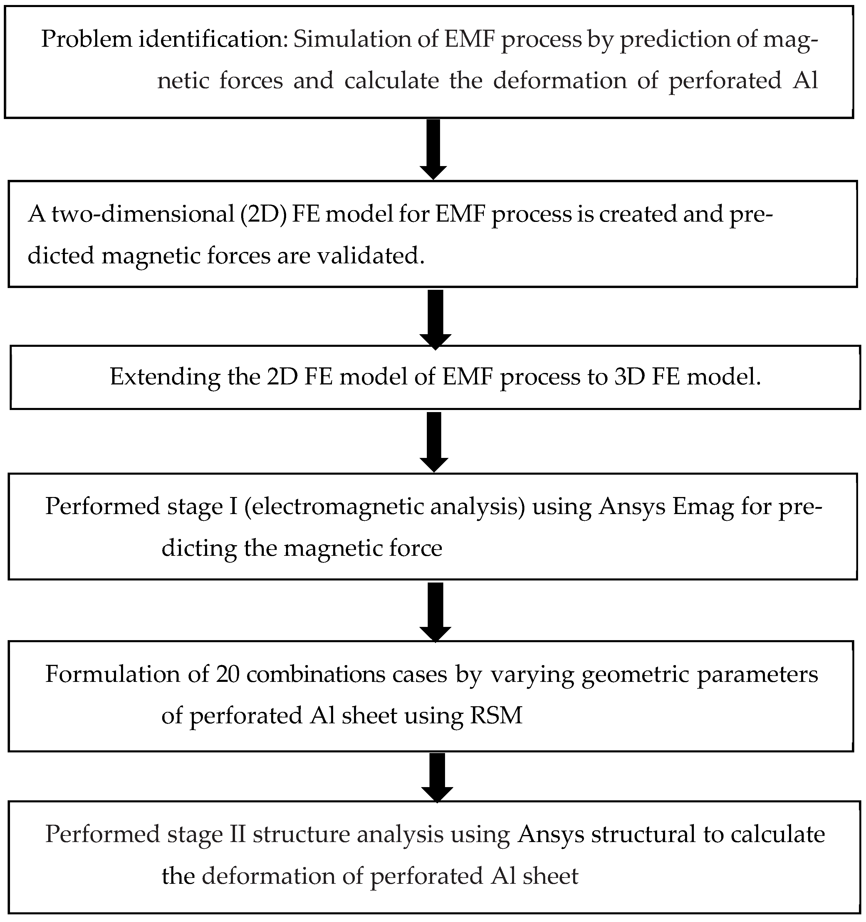
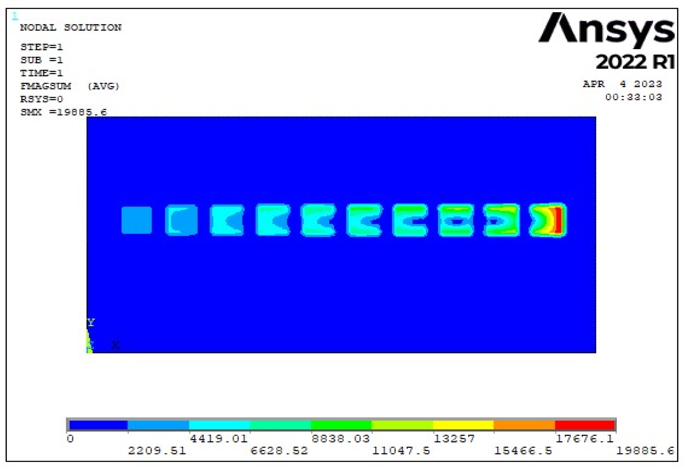
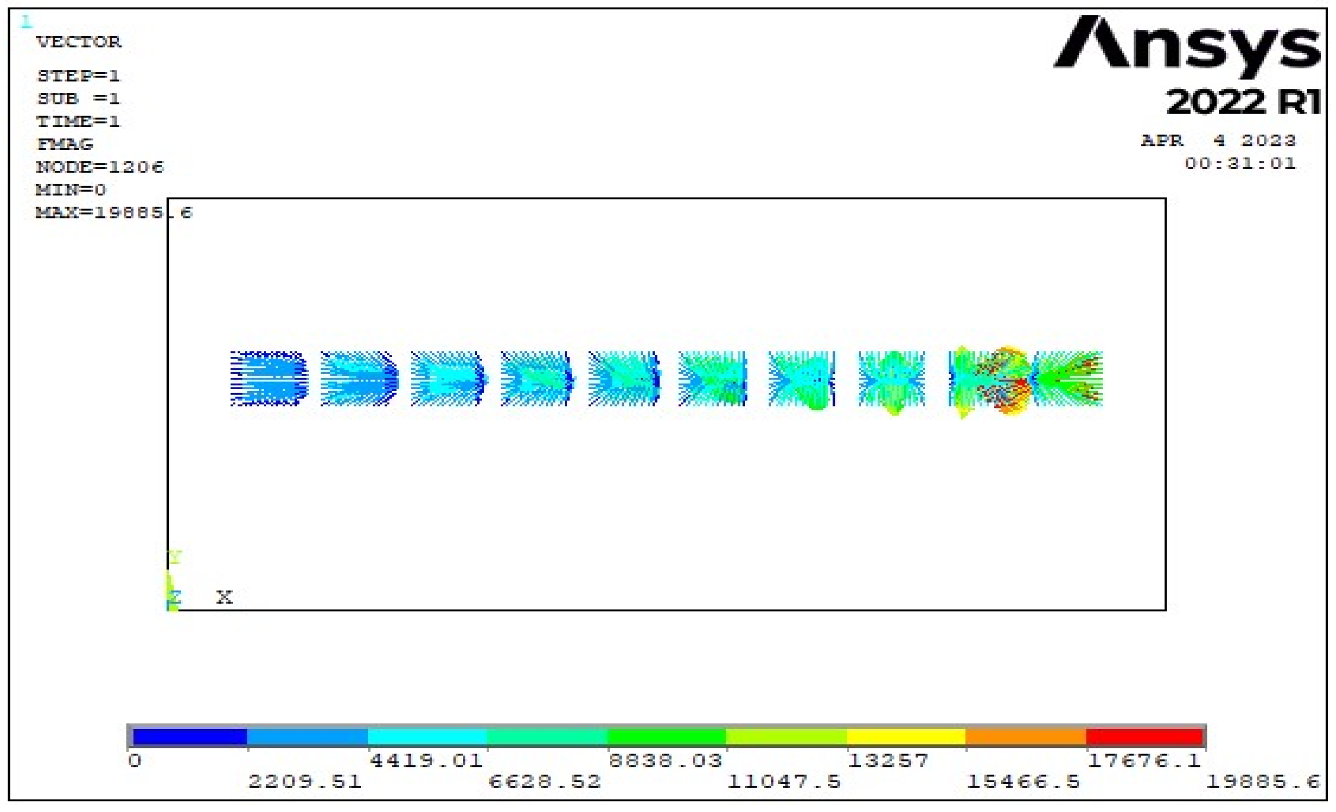
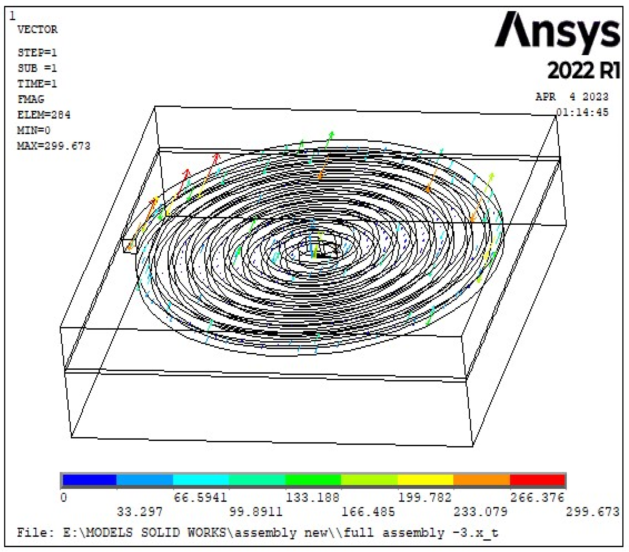
From the literature, it can be concluded that very few researchers have attempted three-dimensional finite element modeling of the EMF process. In this research work, the study and analysis of perforated aluminum sheet metals is carried out by applying the electromagnetic forming process in two stages. In the first stage (electromagnetic analysis), the magnetic force (also called the Lorentz force) is generated by applying current density to the forming coil. In the second stage (structural analysis), the generated Lorentz force is applied to an aluminum 5052 perforated sheet to study deformation.

2. Modeling and Finite Element Simulation

To simulate the electromagnetic forming process, the result of Asati et al. [29] is referred to. Firstly, a two-dimensional (2D) finite element (FE) model is created axi-symmetrically. In order to validate this finite element model, it is compared with the results of Asati et al. [29]. Based on these results, the authors developed a three-dimensional (3D) simulation of the EMF process and calculated the deformation of a perforated aluminum sheet workpiece. Figure 3 shows the flow chart of steps followed.

2.1. Geometric Parameters of the Perforated Sheet

Perforated sheets (dimension 156 mm × 156 mm × 1.5 mm) of a rectangular shape with circular holes are considered for the structural analysis. The modeled commercial aluminum 5052 sheet for the sample (Run 1) is shown in Figure 4. The sheet has a Poisson’s ratio and Young’s modulus of 0.27 and 70 GPa, respectively. Venkatachalam et al. [30] studied the influential geometrical parameters of the perforated sheet, such as the open area percentage, ligament ratio and hole size. The open area is a ratio that reflects how much of the sheet is occupied by holes, normally expressed by a percentage. The ligament ratio is the ratio of ligament width to perforation pitch. Ligament width is the distance between the boundaries of two successive holes, whereas the perforation pitch is the distance between the center points of two successive holes. The open areas considered are 5%, 10%, 15%, 20% and 25%. For the study, ligament ratios of 0.14, 0.2, 0.25, 0.29 and 0.33 are used. The third geometrical measure is the diameter of a circular hole, which is taken as 4 mm, 8 mm, 12 mm, 16 mm and 20 mm.

2.2. Two-Dimensional (2D) Finite Element Model

The electromagnetic forming process simulation and computation of Lorentz force (magnetic force) is achieved using commercial FEA software ANSYS 22 Emag. With reference to literature results from Asati et al. [29], a two-dimensional (2D) FE model is created axi- symmetrically, as shown in Figure 5. The geometric parameters are given in

Table 1. Geometric parameters for 2D model.

Geometric Parameters	Values
Length of the sheet (mm)	156
Thickness of the sheet (mm)	1.5
Number of coils	10
Size of the square coil (mm2)	5 × 5

. Four noded axi-symmetric elements (PLANE13) are used to simulate the mesh coil, workpiece (Sheet) and air region. The material properties that are assigned to simulate the electromagnetic forming process are given in

Table 2. Material properties of finite element model.

Material	Relative Permeability (µ)
Air	1
Copper (for forming coil)	0.999
Aluminum (for metal sheet)	1.003

. In this simulation, the model is discretized into 12,480 elements, with a total number of 12,717 nodes.

The flux parallel boundary conditions are used, and current density (equal to 8000 A/m²) is given as an input to the square-shaped copper coil with 10 turns, which induces a magnetic field. The magnetic force generated due to the forming coil is calculated. Figure 6 shows the meshed model. Figure 7, Figure 8 and Figure 9 illustrate the magnetic force vector sum, a 2D flux line plot and a Vector plot, respectively. In order to validate this finite element model, it is compared with the results of Asati et al. [29], as shown in

Table 3. Comparison of the present finite element model with Asati et al. [29].

Process Parameters	Input Values	Magnetic Force Generated (N)		Error Percentage (%)
		Asati et al. [29]	Present 2D model
Current density (A/m2)	8000	19,923.9	19,885.6	0.192
Gap between sheet and coil (mm)	2
Size of square coil (Length × Height) (mm2)	5

. The error percentage is 0.19%, which shows the accuracy of the present model.

2.3. Three-Dimensional (3D) Finite Element Model

After the validation of the 2D finite element model, the same approach is extended to develop a three-dimensional simulation of the EMF process. The three-dimensional (3D) setup of the EMF system, as shown in Figure 10, is modelled in Solidworks 2021 and imported into ANSYS 22 Emag. The geometry details are given in

Table 4. Geometric parameters for 3D model.

Geometric Parameters	Values
Length of the sheet (mm)	156
Thickness of the sheet (mm)	1.5
Number of turns of coil	10
Cross-section of the square coil (mm2)	5 × 5

. The material properties used are given in

Table 5. Material properties of the 3D finite element model.

Material	Relative Permeability (µ)
Air	1
Copper (for forming coil)	0.999
Aluminum (for metal sheet)	1.003

.

ANSYS 22 Emag software is used to simulate the 3D electromagnetic simulation. The electromagnetic force is generated after the current excitation of the forming coil. Figure 11 represents the finite element model of the EMF process. A SOLID97 element is used for meshing the forming coil, the Al sheet and the air region so that a magnetic field is propagated in the region. Over the outer surface area, the flux parallel boundary condition is provided. As shown in Figure 12, a magnetic field is created when a square-shaped copper coil with 10 turns is subjected to a current density of 13.75 × 10⁶ A/m², which produces a Lorentz force of 300 N in the area. This force is given to a perforated aluminum sheet in the structural analysis to determine the sheet’s deformation.

3. Structural Analysis

3.1. Design of Experiments and Optimization

In the RSM designs, the CCD (central composite design) is the most widely used design. In a minimum number of runs, it provides much information on variable effects and overall error. It consists of 20 points with 6 axial and 8 corner points. Five different levels of all three parameters are set. The levels of all three parameters are categorized as −2, −1, 0, 1 and 2 (

Table 6. Geometric parameter levels.

Factors	Levels
	−2	−1	0	1	2
Open area (%)	5	10	15	20	25
Ligament Ratio	0.14	0.2	0.25	0.29	0.33
Hole size (mm)	4	8	12	16	20

). In Figure 13, the CCD with 20 simulation runs is shown. The influential geometric parameters of the perforated sheet are considered to be the open area percentage, ligament ratio and size of the hole. To perform the simulation, 20 different combinations (Runs) of open area percentage, ligament ratio and size of hole are found with the help of the DOE method. For each of these open area percentage, ligament ratio and size of the hole parameters, five different levels are considered. As depicted in Figure 13, the response surface methodology’s central composite design (CCD) is employed.

After the end of stage I (electromagnetic analysis), the Lorentz force is obtained, and stage II (structural analysis) is used to determine the deformation and stresses in the sheet following the forming process. The generated Lorentz force from stage I is then applied to a perforated sheet to determine the deformation. The outcomes for Run 1 are shown in Figure 14.

Figure 15 depicts the three-dimensional finite element model of the perforated aluminum sheet for Run 1. Solidworks 2021 software is used to build the geometric model, which is then imported into ANSYS 22 software. The nonlinear material properties of an Al 5052 sheet with a Poisson’s ratio of 0.27 are included in numerical model.

The DOE table, i.e.,

Table 7. DOE table representing different combinations and corresponding sheet deformation.

Run	Open Area (%)	Ligament Ratio	Hole Size (mm)	Deformation (mm) × (10−3)
1	25	0.25	12	3.6
2	15	0.25	20	0.75
3	5	0.25	12	0.61
4	10	0.29	8	1.7
5	15	0.25	12	1.4
6	15	0.25	12	1.4
7	15	0.14	12	5.8
8	10	0.2	8	2.2
9	15	0.25	12	1.4
10	15	0.25	4	5.4
11	15	0.25	12	1.4
12	10	0.29	16	0.53
13	15	0.25	12	1.4
14	20	0.2	8	18.5
15	15	0.33	12	1.1
16	15	0.25	12	1.4
17	20	0.29	16	1
18	20	0.29	8	5.7
19	10	0.2	16	0.9
20	20	0.2	16	1.6

, gives the number of simulations to be performed, and accordingly, the geometric models are created. With the help of ANSYS structural, the obtained Lorentz force (i.e., 300 N) from stage I (electromagnetic analysis) is applied, and the corresponding deformation is calculated for each sample model (combinations or runs). To determine the impact of three input geometrical parameters, namely the open area percentage, ligament ratio, and hole size, on the response parameter, i.e., deformation, the analysis of variance (ANOVA) technique is used.

Table 8. ANOVA results.

Source	DF	Adj SS	Adj MS	F-Value	p-Value
Model	9	0.000255	0.000028	5.14	0.009
Linear	3	0.000078	0.000026	4.72	0.027
Open area (%)	1	0.000041	0.000041	7.53	0.021
Ligament ratio	1	0.000005	0.000005	0.96	0.351
Hole size (mm)	1	0.000008	0.000008	1.44	0.257
Square	3	0.000010	0.000003	0.62	0.616
Open area (%) × Open area (%)	1	0.000002	0.000002	0.40	0.543
Ligament ratio × Ligament ratio	1	0.000005	0.000005	0.87	0.373
Hole size (mm) × Hole size (mm)	1	0.000007	0.000007	1.31	0.278
2-Way interaction	3	0.000090	0.000030	5.41	0.018
Open area (%) × Ligament ratio	1	0.000022	0.000022	4.04	0.072
Open area (%) × Hole size (mm)	1	0.000046	0.000046	8.30	0.016
Ligament ratio × Hole size (mm)	1	0.000021	0.000021	3.90	0.077
Error	10	0.000055	0.000006
Lack-of-Fit	5	0.000055	0.000011
Pure error	5	0.000000	0.000000
Total	19	0.000310

Where Adj SS—adjusted some of squares, DF–degrees of freedom, Adj MS—adjusted mean squares, with p-value guides to find the significance of results. The F-value helps to decide whether to “accept or reject” the hypothesis.

displays the ANOVA findings. A regression equation that describes the connection between the response parameter and the input parameters is produced from the ANOVA. It also shows the relationships between the variables of the model. The ANOVA is performed with the help of MINITAB 19 software.

3.2. Regression Equation

The regression equation (Equation (8)) is a second-order polynomial equation obtained through MINITAB software. In this regression equation, the deformation of the Al sheet is calculated by substituting the corresponding values of open area percentage, ligament ratio and size of the hole for different samples, as shown in

Table 9. DOE table showing different combinations and deformation and error percentage.

Run	Open Area (%)	Ligament Ratio	Hole Size (mm)	Deformation (mm) × (10−3)		Error (%)
				Finite Element Simulation	Regression Equation
1	25	0.25	12	3.6	3.98	9.54
2	15	0.25	20	0.75	0.714	3.46
3	5	0.25	12	0.61	0.624	2.24
4	10	0.29	8	1.7	1.68	1.17
5	15	0.25	12	1.4	1.51	7.28
6	15	0.25	12	1.4	1.51	7.28
7	15	0.14	12	5.8	6.3	8.62
8	10	0.2	8	2.2	2.5	1.01
9	15	0.25	12	1.4	1.51	7.28
10	15	0.25	4	5.4	6.1	10
11	15	0.25	12	1.4	1.51	7.28
12	10	0.29	16	0.53	0.49	9.43
13	15	0.25	12	1.4	1.51	7.28
14	20	0.2	8	18.5	17.2	7.02
15	15	0.33	12	1.1	1	9.03
16	15	0.25	12	1.4	1.51	7.28
17	20	0.29	16	1	0.98	2
18	20	0.29	8	5.7	5.91	9.98
19	10	0.2	16	0.9	0.89	1.9
20	20	0.2	16	1.6	1.75	9.3

. Table 9 also contains the error percentage between the sheet deformation calculated from the finite element simulation (ANSYS Emag) and the regression equation.

Deformation (mm) = 0.0077 + 0.00325 A − 0.124 B − 0.00178 C+ 0.000012 A² + 0.196 B²
+ 0.000034 C² − 0.00739 AB − 0.000120 AC + 0.00908 BC

(8)

where A = percentage of open area, B = ligament ratio, and C = hole size.

Regression model compatibility is tested by comparing it with FEA findings. The error calculated between the regression model and the finite element simulation pertaining to the deformation value is less than 10%, which shows the legitimacy of regression model.

Figure 16 shows the influence of different parameters on sheet deformation. Figure 17 shows the maximum deformation generated when the percentage of open area ranges from 20 to 25%, with respect to a variation of ligament ratio from 0.2 to 0.25.

In Figure 18, the contour plot helps to identify the effect of open area (%) and hole size on deformation. Figure 19 shows that maximum deformation is generated for hole sizes ranging from 4 to 8 mm.

3.3. Response Optimization

The MINITAB software is used to carry out study on response optimization. It predicts the optimized combination of variables that optimizes a single or multiple responses. As shown in Figure 20, it helps to observe the effect of multiple variables on response. After the optimized values are obtained from MINITAB, they are again checked and validated with finite element simulation. The maximum deformation (equal to 0.0435 mm) is calculated for the optimized combination of 25% open area, 0.14 LR and 4 mm hole size, as shown in

Table 10. Response optimization results.

Variable			Setting
Open area (%)			25
Ligament ratio			0.14
Hole size (mm)			4
Response	Fit	SE Fit	95% CI	95% PI
Deformation (mm)	0.04351	0.00757	(0.02664, 0.06038)	(0.02585, 0.06118)

. The deformation is also calculated for this optimized combination in ANSYS Emag, and is equal to 0.0419 mm. The error for deformation calculated by optimized combination in MINITAB (0.0435 mm) and FE simulation (0.0419 mm) is 4%, which shows worthiness of optimized model (Figure 21).

4. Conclusions

In this research work, a three-dimensional (3D) model for the EMF process is developed by extending a validated 2D axisymmetric model to three dimensions. In terms of the EMF process, experimental studies are usually very expensive, whereas numerical analyses are much more cost-effective and enable a wider range of parameters to be investigated quickly. The deformation of the perforated Al sheet is caused due to the magnetic force generated, which is then calculated by finite element simulation of the EMF process. The DOE/RSM approach is used to investigate the influences of the geometric parameters of the perforated sheet (i.e., the open area percentage, ligament ratio and size of the hole). For 20 different combinations, finite element simulations are performed, and the corresponding deformation is calculated. These finite element results are compared with the deformation calculated by a regression equation developed through ANOVA, which gives less than 10% error, showing the accuracy of the regression model. It is concluded that the optimized combination of 25% open area, 0.14 LR and 4 mm hole size gives the maximum deformation of the sheet, equal to 0.0435 mm. The confirmation simulation is carried out to validate the optimization study, showing good agreement (error percentage = 4%) with the optimized regression model, which will help by saving lot of time in future designs.

References

1. Daehn, G.S. High Velocity Metal Forming, ASM Handbook of Forming and Forging; ASM International: Materials Park, OH, USA, 2003. [Google Scholar]
2. Furth, H.; Waniek, R. New ideas on magnetic forming. Am. Mach. Metalwork. Manuf. 1962, 106, 92–95. [Google Scholar]
3. Kleiner, M.; Beerwald, C.; Homberg, W. Analysis of Process Parameters and Forming Mechanisms within the Electromagnetic Forming Process. CIRP Ann. Manuf. Technol. 2005, 54, 225–228. [Google Scholar] [CrossRef]
4. Meriched, A.H.; Feliachi, M.; Mohellebi, H. Electromagnetic Forming of Thin Metal Sheets. IEEE Trans. Magn. 2000, 36, 1804–1807. [Google Scholar] [CrossRef]
5. Fenton, G.; Deahn, G.S. Modeling of electromagnetically formed sheet metal. J. Mater. Process Technol. 1998, 75, 6–16. [Google Scholar] [CrossRef]
6. Cao, Q.; Li, L.; Lai, Z.; Zhou, Z.; Xiong, Q.; Zhang, X.; Han, X. Dynamic analysis of electromagnetic sheet metal forming process using finite element method. Int. J. Adv. Manuf. Technol. 2014, 74, 361–368. [Google Scholar] [CrossRef]
7. Reese, S.; Svendsen, B.; Stiemer, M.; Unger, J.; Schwarze, M.; Blum, H. On a new finite element technology for electromagnetic metal forming processes. Arch. Appl. Mech. 2005, 74, 834–845. [Google Scholar] [CrossRef]
8. Mamalis, A.G.; Manolakos, D.E.; Kladas, A.G.; Koumoutsos, A.K. On the electromagnetic sheet metal forming: Numerical simulation. AIP Conf. Proc. Am. Inst. Phys. 2004, 712, 778–783. [Google Scholar]
9. Luca, D. Finite element modeling and experiment for behavior estimation of AlMn0.5Mg0.5 sheet during electromagnetic forming. Trans. Nonferrous Met. Soc. China 2015, 25, 2331–2341. [Google Scholar] [CrossRef]
10. Siddiqui, M.A.; Correia, J.P.M.; Ahzi, S.; Belouettar, S. A numerical model to simulate electromagnetic sheet metal forming process. Int. J. Mater. Form. 2008, 1 (Suppl. S1), 1387–1390. [Google Scholar] [CrossRef]
11. Unger, J.; Stiemer, M.; Svendsen, B.; Blum, H. Multifield modeling of electromagnetic metal forming processes. J. Mater. Process. Technol. 2006, 177, 270–273. [Google Scholar] [CrossRef]
12. Deng, J.; Li, C.; Zhao, Z.; Tu, F.; Yu, H. Numerical simulation of magnetic flux and force in electromagnetic forming with attractive force. J. Mater. Process. Technol. 2007, 184, 190–194. [Google Scholar] [CrossRef]
13. Khandelwal, R.; Dabade, U.A. Performance Analysis of Electromagnetic Forming Process; GRIN Verlag: München, Germany, 2015. [Google Scholar]
14. Imbert, J.M.; Winkler, S.L.; Worswick, M.J.; Golovashchenko, S. Formability and Damage in Electromagnetically Formed AA5754 and AA6111. In Proceedings of the 1st International Conference on High Speeding Forming, Dortmund, Germany, 31 March–1 April 2004; pp. 201–210. [Google Scholar]
15. Parez, I.; Aranguren, I.; Gonzlez, B.; Eguia, I. Electromagnetic forming: A new coupling method. Int. J. Mater. Form. 2009, 2, 637–640. [Google Scholar] [CrossRef]
16. Siddiqui, M.A.; Correia, J.P.M.; Ahzi, S.; Belouettar, S. Electromagnetic forming process: Estimation of magnetic pressure in tube expansion and numerical simulation. In Proceedings of the 12th ESAFORM Conference on Material Forming, Enschede, The Netherlands, 27–29 April 2009; pp. 27–29. [Google Scholar]
17. Bahmani, M.A.; Niayesh, K.; Karimi, A. 3D Simulation of magnetic field distribution in electromagnetic forming systems with field-shaper. J. Mater. Process. Technol. 2009, 209, 2295–2301. [Google Scholar] [CrossRef]
18. Haiping, Y.U.; Chunfeng, L.I.; Jianghua, D.E.N.G. Sequential coupling simulation for electromagnetic mechanical tube compression by finite element analysis. J. Mater. Process. Technol. 2009, 209, 707–713. [Google Scholar] [CrossRef]
19. Xu, W.; Liu, X.S.; Yang, J.G.; Fang, H.Y.; Xu, D.; Xu, W.L. Meshing and choice of evaluating parameters of results in simulation of electromagnetic force for forming of sheet metal. J. Mater. Process. Technol. 2009, 209, 3320–3324. [Google Scholar] [CrossRef]
20. Ahmed, M.; Panthi, S.K.; Ramakrishnan, N.; Jha, A.K.; Yegneswaran, A.H.; Dasgupta, R. Alternative flat coil design for electromagnetic forming using FEM. Trans. Nonferrous Met. Soc. China 2011, 21, 618–625. [Google Scholar] [CrossRef]
21. Psyk, V.; Risch, D.; Kinsey, B.L.; Tekkaya, A.E.; Kleiner, M. Electromagnetic forming—A review. J. Mater. Process. Technol. 2011, 211, 787–829. [Google Scholar] [CrossRef]
22. Bhole, K.S.; Kale, B.S.; Deshmukh, P.D.; Sonare, O.G. Numerical Analysis and Investigation of Aluminum Alloys in Electromagnetic Metal Forming Process. Int. J. Technol. Eng. Syst. 2011, 2, 98–102. [Google Scholar]
23. Qiu, L.; Han, X.; Xiong, Q.; Zhou, Z.; Li, L. Effect of Workpiece Motion on Forming Velocity in Electromagnetic Forming. In Proceedings of the 5th International Conference on High-Speed Forming, Dortmund, Germany, 24–26 April 2012; Volume 12800, pp. 103–112. [Google Scholar]
24. Abdelhafeez Ali, M.; Nemat-Alla, M.M.; El-Sebaie, M.G. Finite element analysis of electromagnetic bulging of sheet metal. Int. J. Sci. Eng. Res. 2012, 3, 1–7. [Google Scholar]
25. Takatsu, N.; Kato, M.; Sato, K.; Tobe, T. High-speed forming of metal sheets by electromagnetic force. JSME Int. J. Vib. Control. Eng. Eng. Ind. 1988, 31, 142–148. [Google Scholar] [CrossRef]
26. Zhang, X.; Huang, Y.; Wang, Y.; Shen, W.; Cui, J.; Li, G.; Deng, H. Numerical simulation and experimental study on electromagnetic punching-flanging process of 6061 aluminum alloy sheets. J. Manuf. Process. 2022, 84, 902–912. [Google Scholar] [CrossRef]
27. Xu, J.; Huang, L.; Hong, X.; Liu, X.; Su, H.; Ma, F.; Li, J. Research on the electromagnetic blanking based on force-free region deformation: Simulation and experiments. Int. J. Adv. Manuf. Technol. 2020, 108, 1751–1766. [Google Scholar] [CrossRef]
28. Li, H.W.; Yan, S.L.; Zhan, M.; Zhang, X. Eddy current induced dynamic deformation behaviors of aluminum alloy during EMF: Modeling and quantitative characterization. J. Mater. Process. Technol. 2019, 263, 423–439. [Google Scholar] [CrossRef]
29. Asati, R.; Pradhan, S.K. Two-stage Finite Element simulation to predict deformation and stresses in Electromagnetic Formed component. Procedia Manuf. 2017, 12, 42–58. [Google Scholar] [CrossRef]
30. Venkatachalam, G.; Narayanan, S.; Sathiyanarayanan, C. A finite element method-based formability analysis of triangular pattern of square hole perforated commercial pure aluminium sheets. Int. J. Mech. Mater. Eng. 2012, 7, 209–213. [Google Scholar]
Figure 1. (a) Schematic representation of the EMF process (b) Set- up of the EMF process.
Mathematics 11 01983 g001
Figure 2. Electromagnetic flat sheet forming.
Mathematics 11 01983 g002
Figure 3. Flow chart of the research work.
Mathematics 11 01983 g003
Figure 4. Perforated sheet (for Run 1).
Mathematics 11 01983 g004
Figure 5. Finite element model.
Mathematics 11 01983 g005
Figure 6. 2D Meshed model.
Mathematics 11 01983 g006
Figure 7. The magnetic force vector sum.
Mathematics 11 01983 g007
Figure 8. 2D flux lines.
Mathematics 11 01983 g008
Figure 9. Vector plot.
Mathematics 11 01983 g009
Figure 10. Three-dimensional setup of the Al sheet, forming the coil and air regions.
Mathematics 11 01983 g010
Figure 11. 3D Meshed model.
Mathematics 11 01983 g011
Figure 12. Magnetic force generated.
Mathematics 11 01983 g012
Figure 13. Central composite design.
Mathematics 11 01983 g013
Figure 14. Deformed sheet.
Mathematics 11 01983 g014
Figure 15. 3D finite element model (for Run 1).
Mathematics 11 01983 g015
Figure 16. Main effects plot showing influences of different parameters on the sheet deformation.
Mathematics 11 01983 g016
Figure 17. Influence of percentage of open area and ligament ratio.
Mathematics 11 01983 g017
Figure 18. Influence of percentage of open area and hole size.
Mathematics 11 01983 g018
Figure 19. Influence of ligament ratio and hole size.
Mathematics 11 01983 g019
Figure 20. Influence of ligament ratio and hole size (for optimized model).
Mathematics 11 01983 g020
Figure 21. Response optimization of different parameters.
Mathematics 11 01983 g021