
Design of Continuous Finite-Time Controller Based on Adaptive Tuning Approach for Disturbed Boost Converters
 ,
,  ,
,  , and
, and
Abstract
:1. Introduction
- A novel adaptive continuous finite-time controller is designed for disturbed boost converter systems in the presence of white noise and model uncertainty;
- A design method which guarantees the convergence and maintenance of the system state trajectories to a predefined neighbourhood of the origin in the finite time;
- Estimating the disturbance boundaries using an adaptive continuous scheme to adjust the controller adaptation gain;
- Eliminating the chattering phenomenon using a switching function based on a continuous adaptation gain.
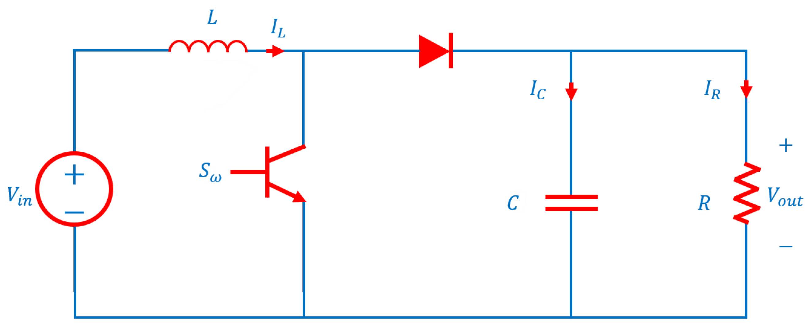
2. DC–DC Boost Converter
- (a)
- is positive-definite;
- (b)
- time derivative of at is negative-definite;
- (c)
- There are positive real values and , and a neighbourhood of origin such that:
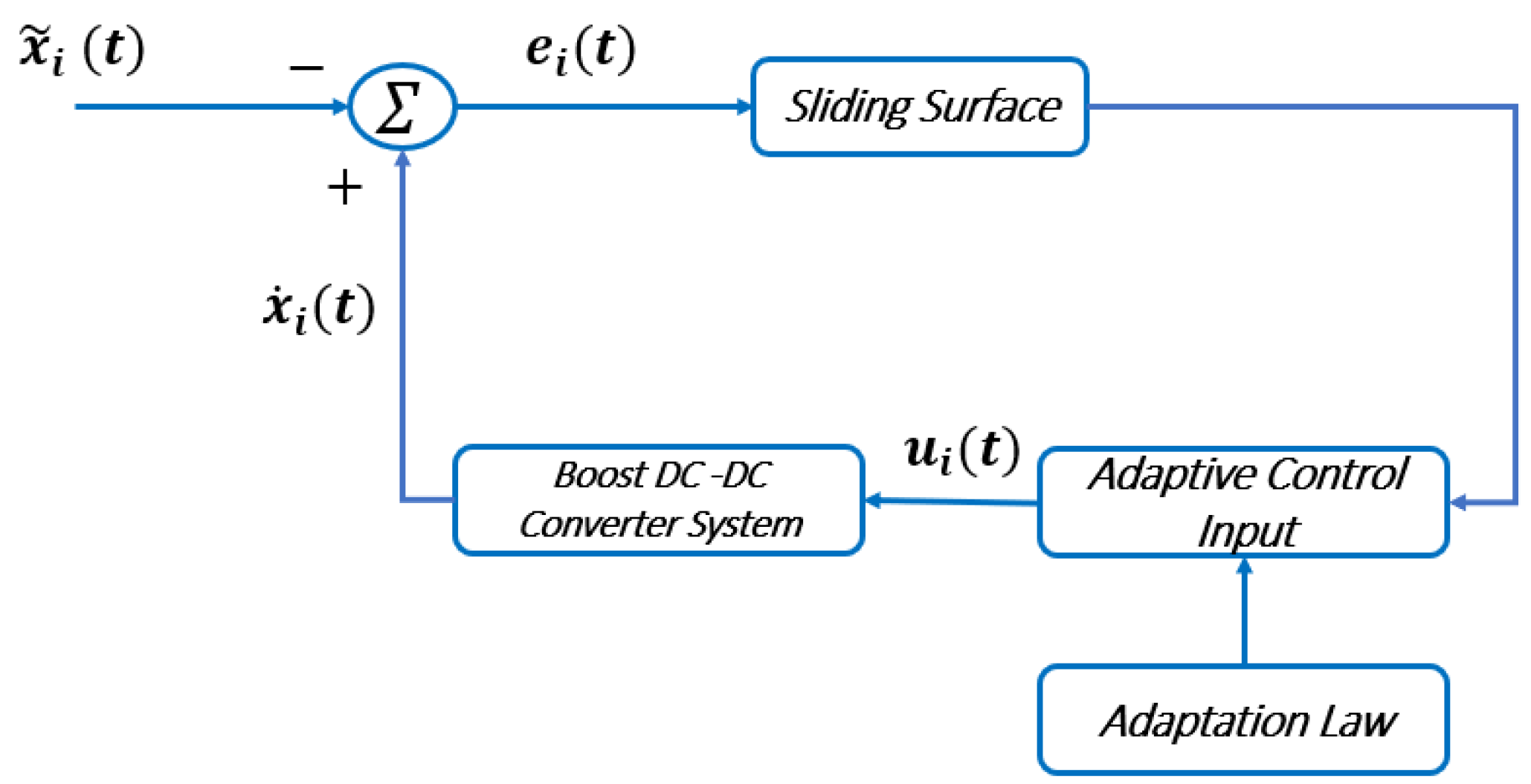
3. Control Design
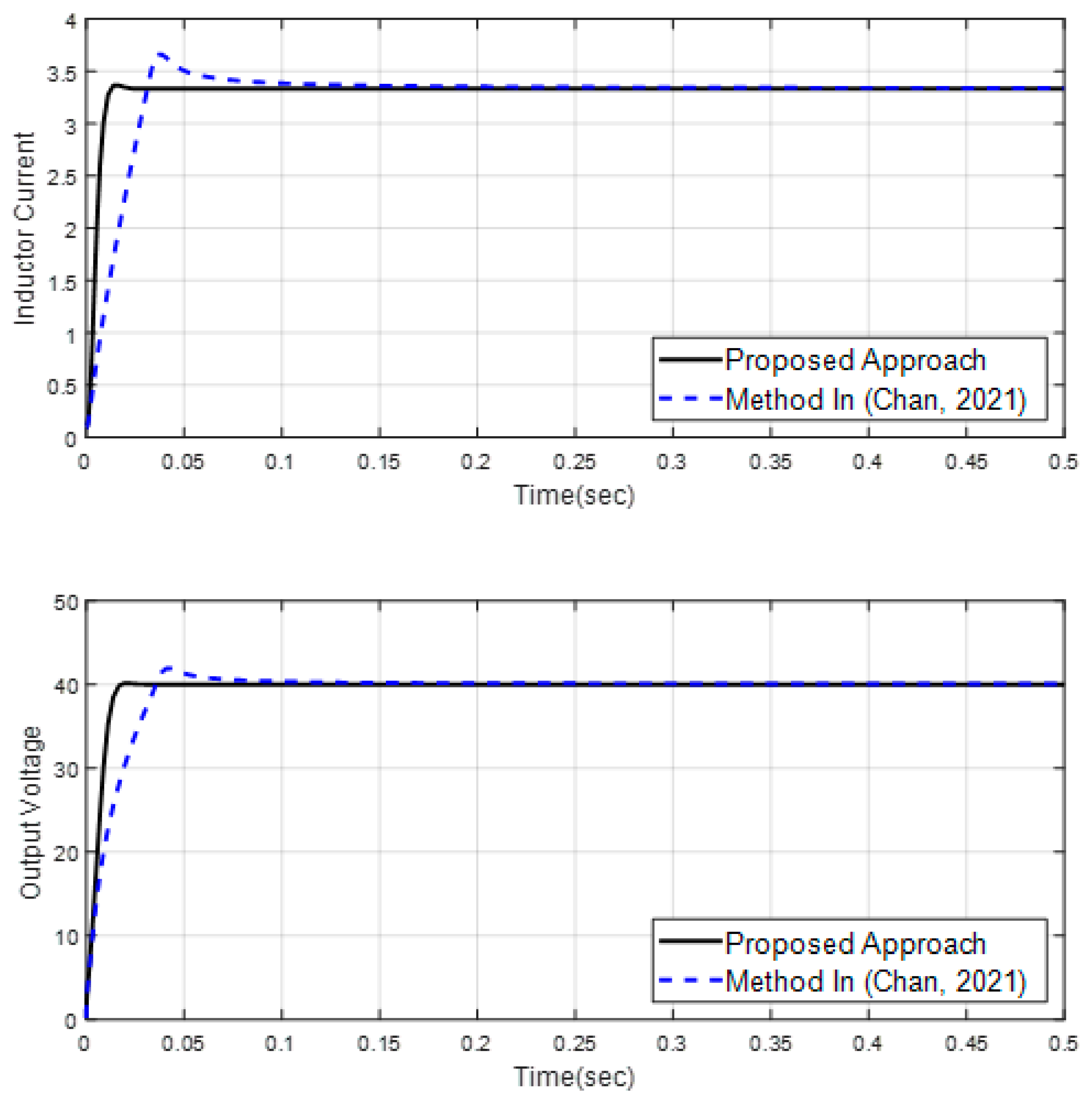
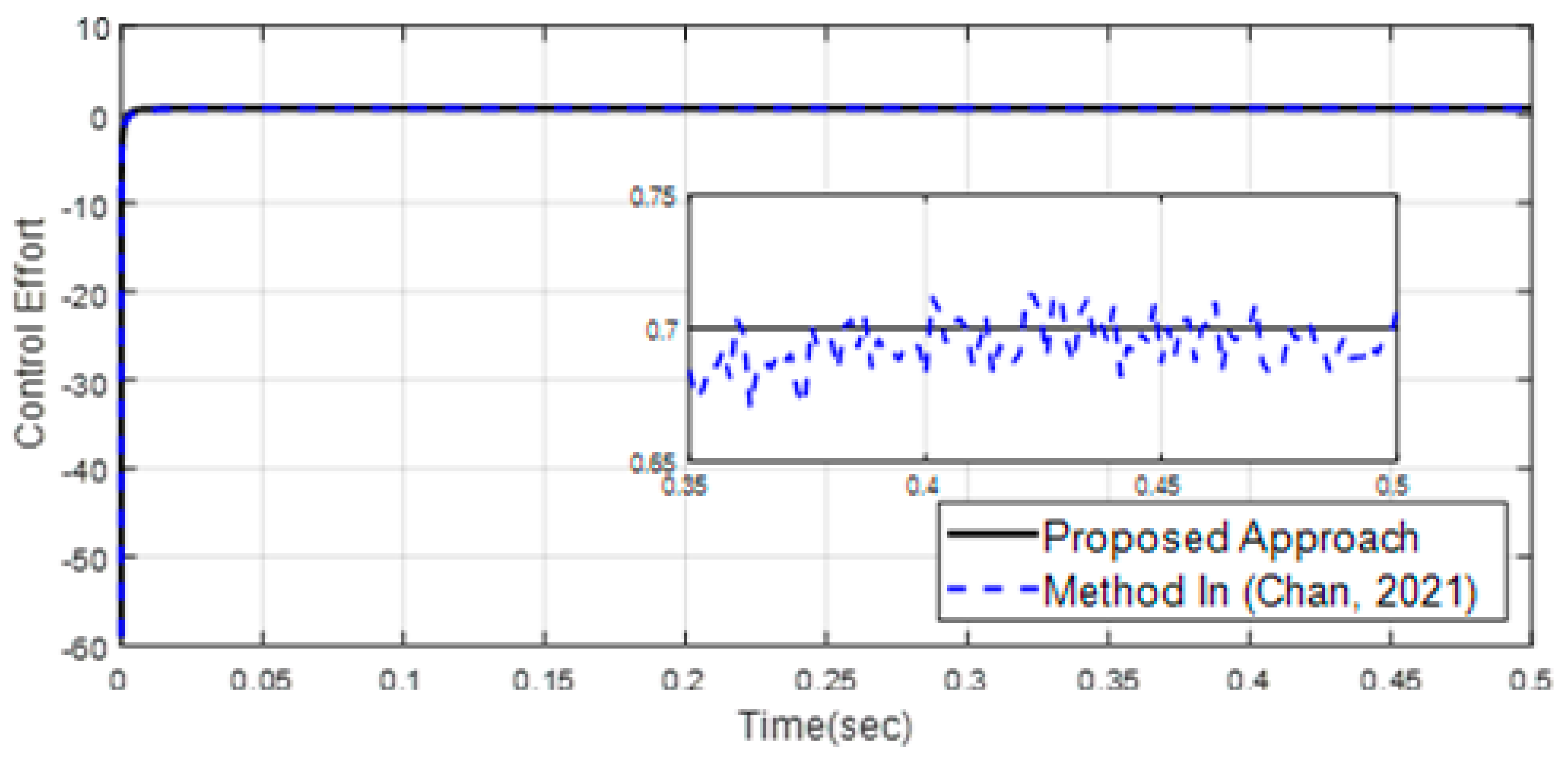
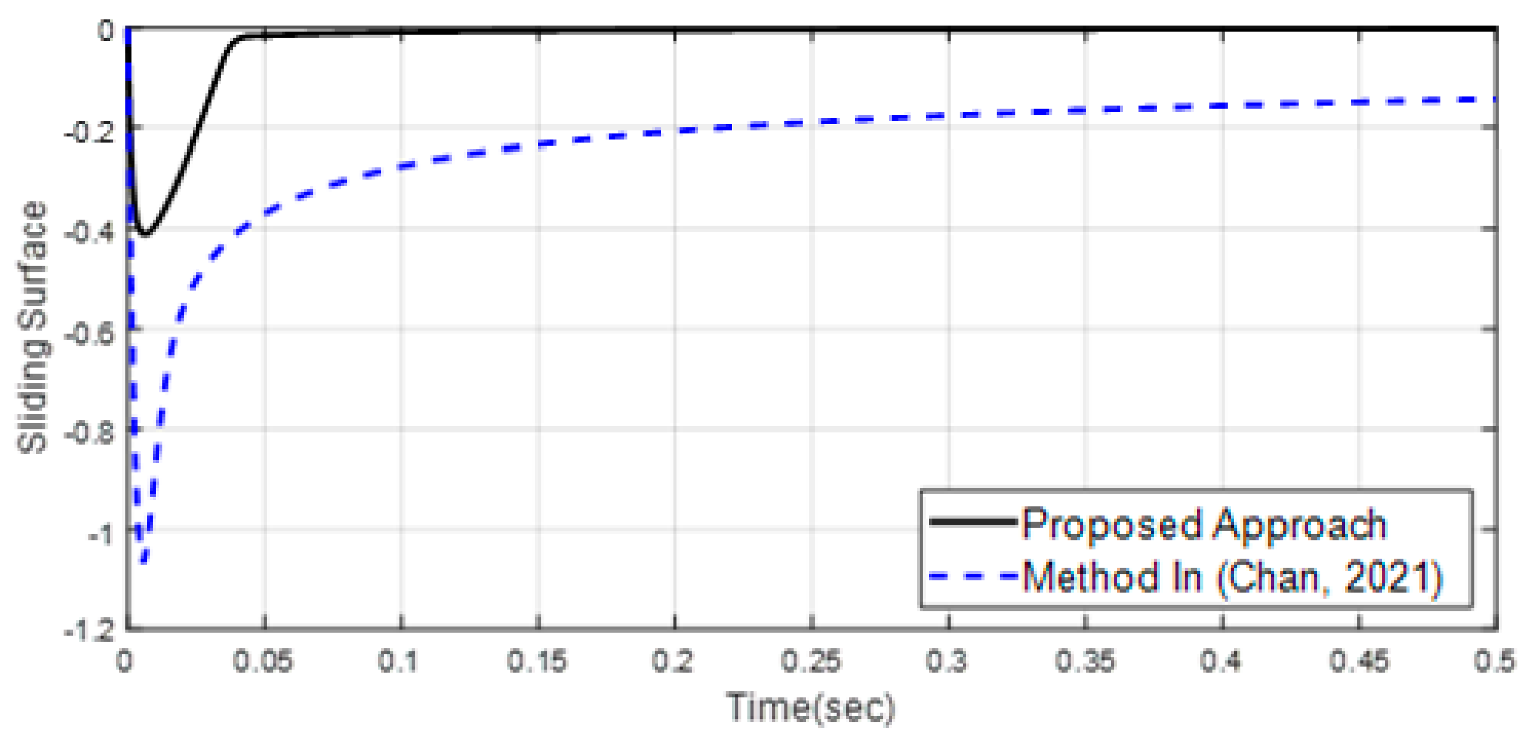
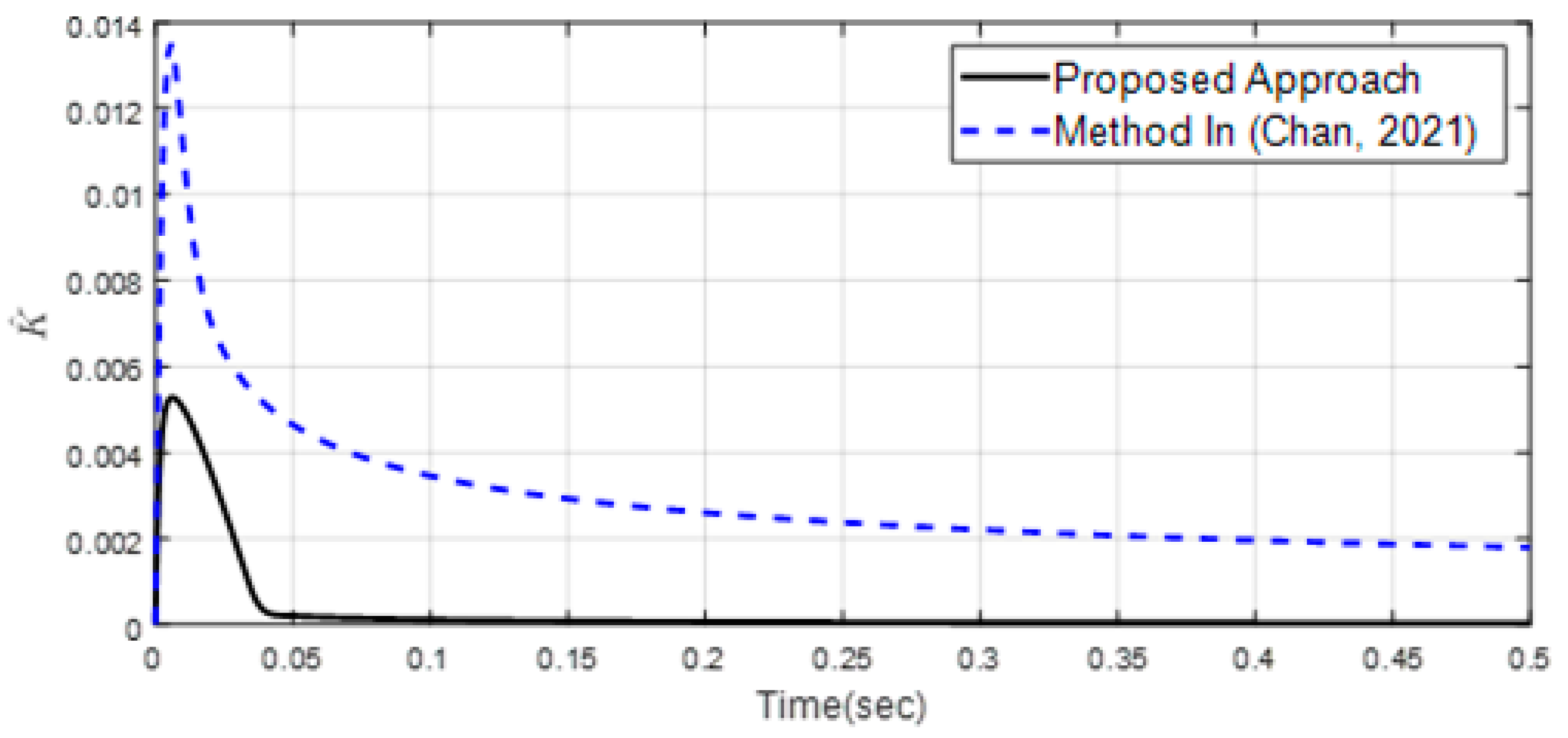
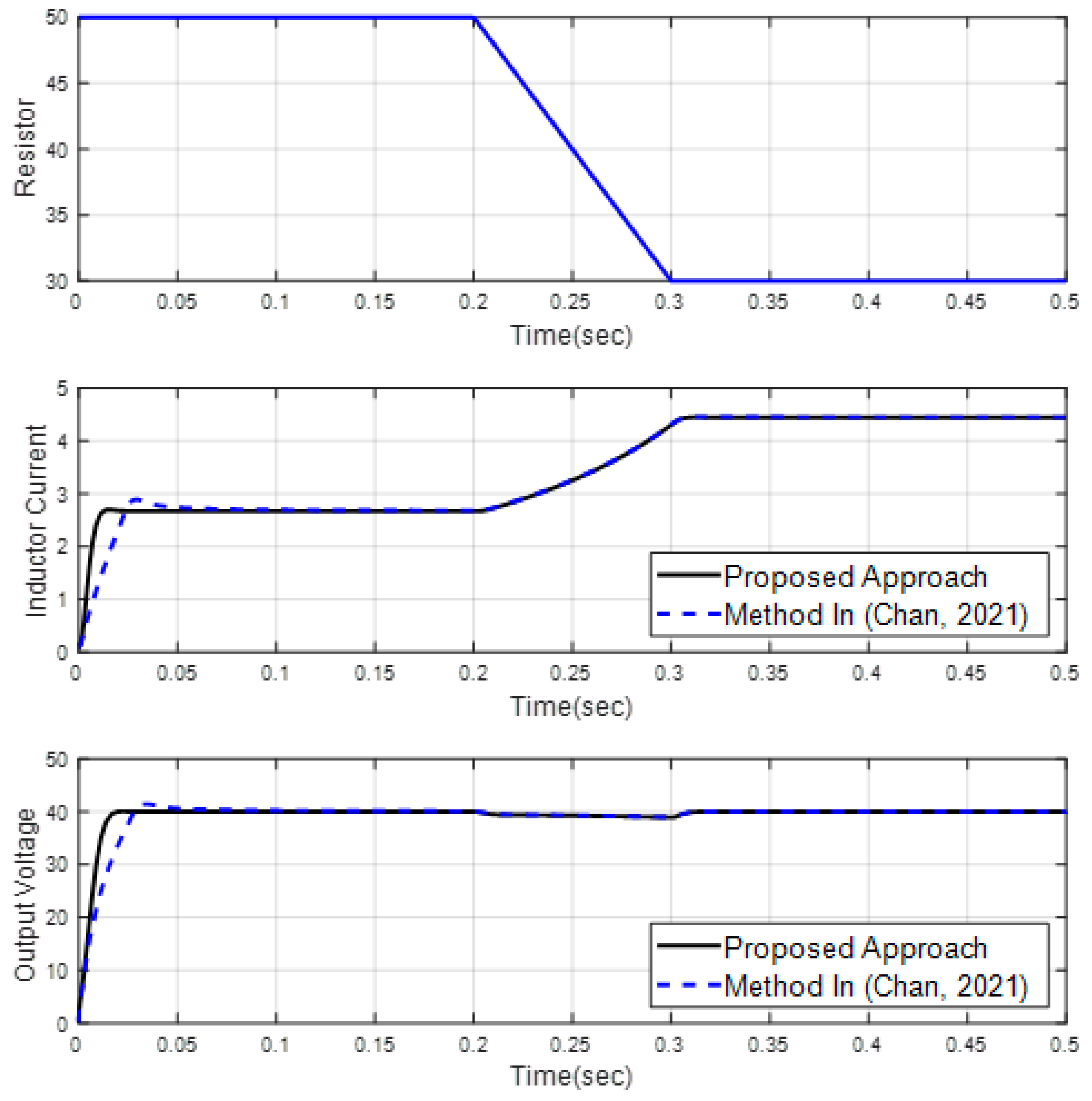
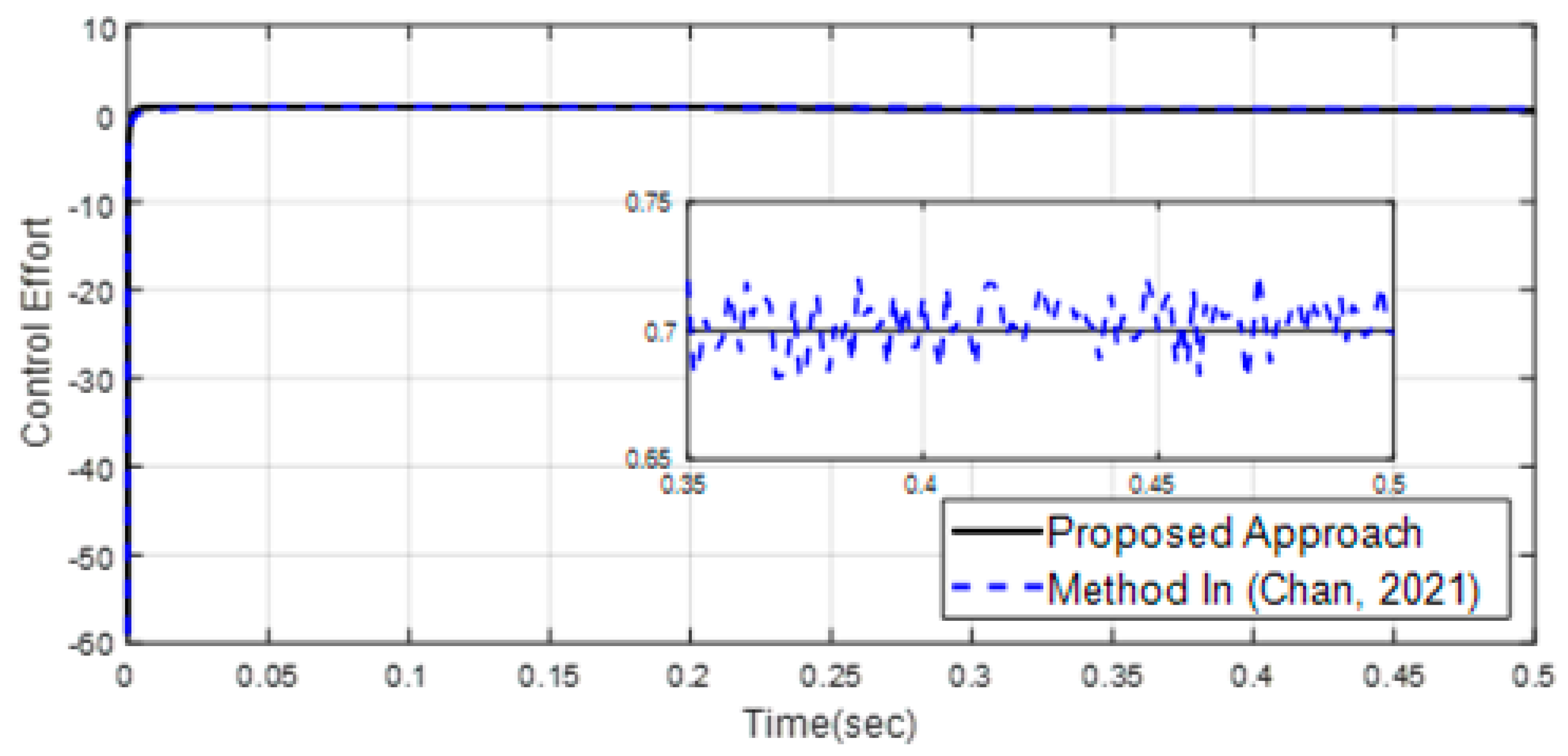
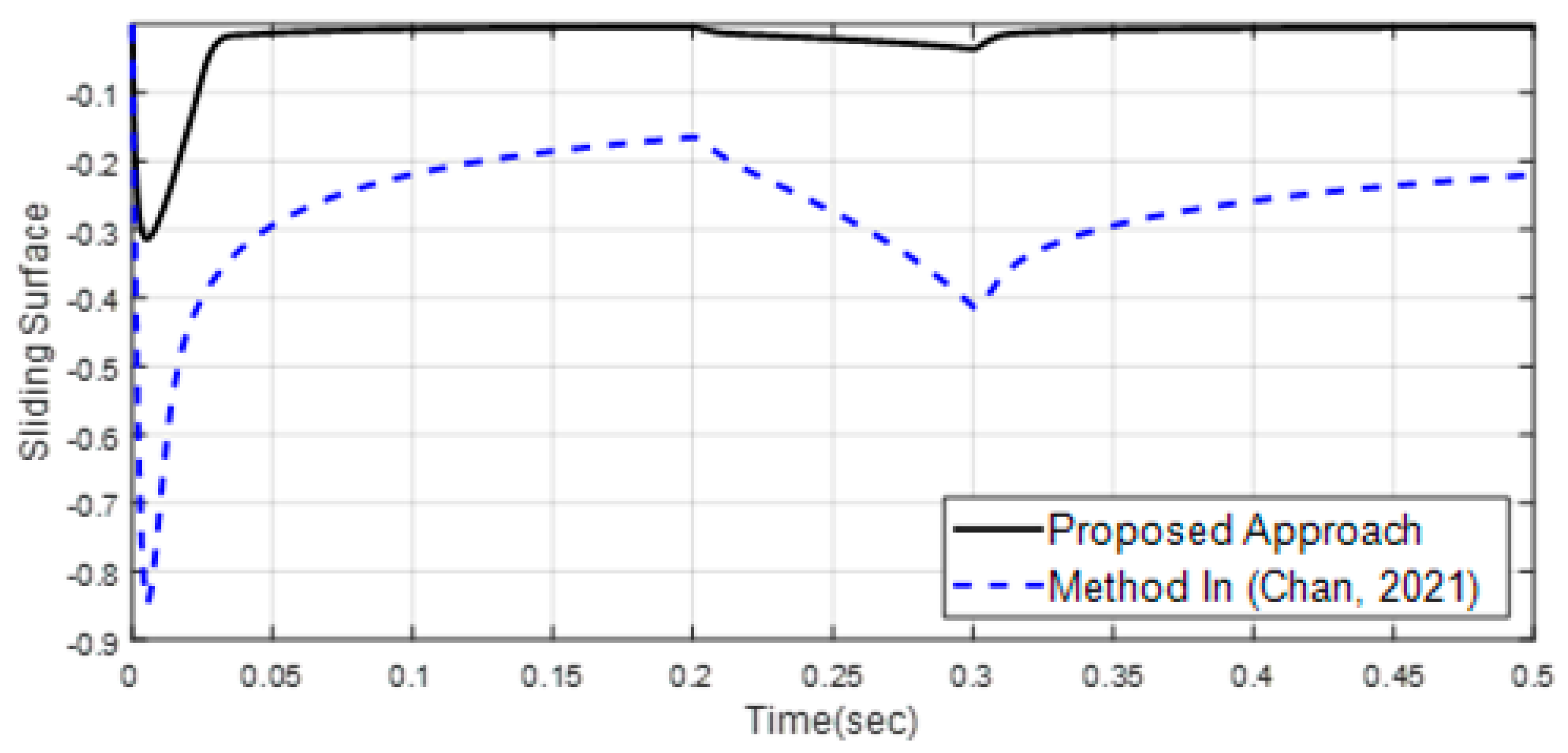
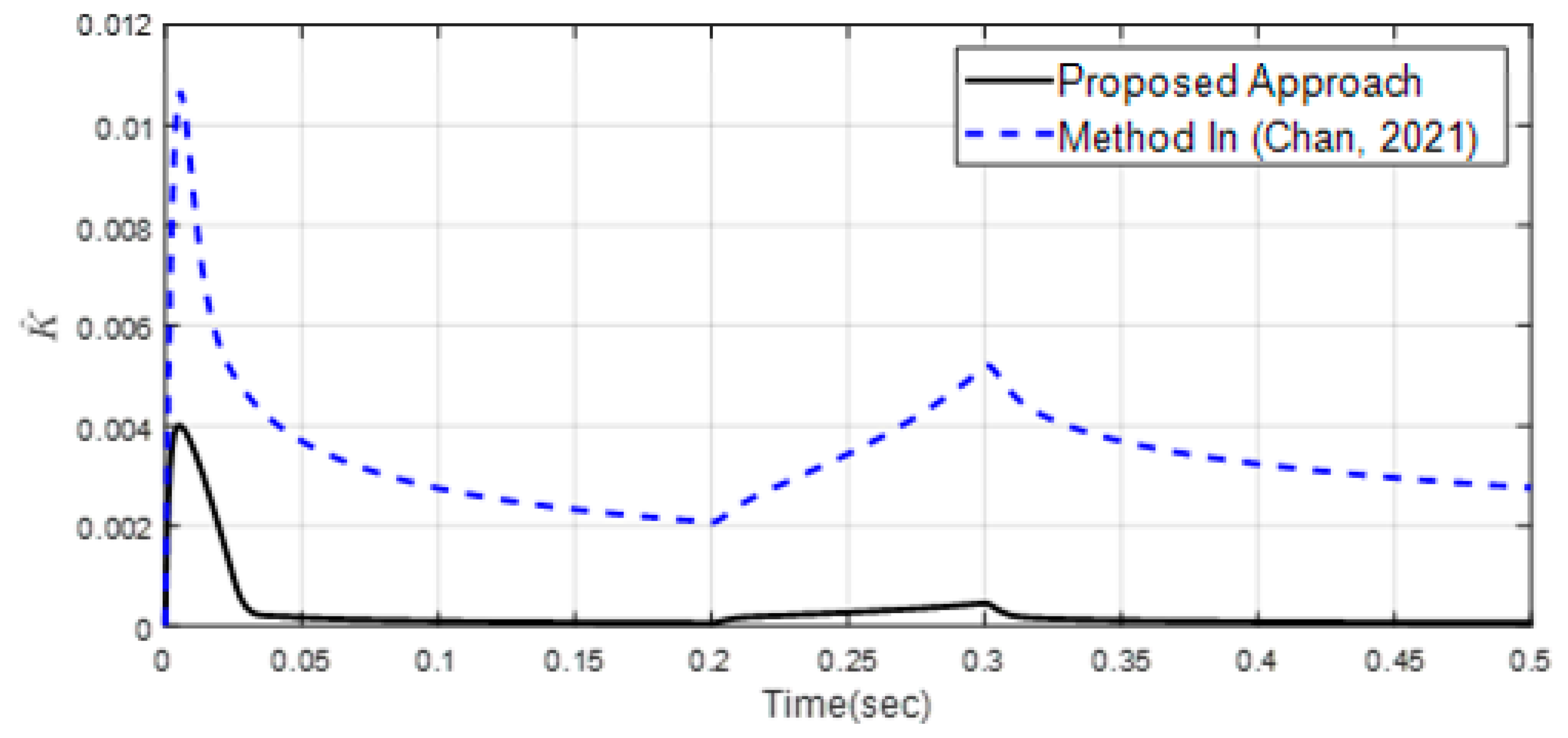
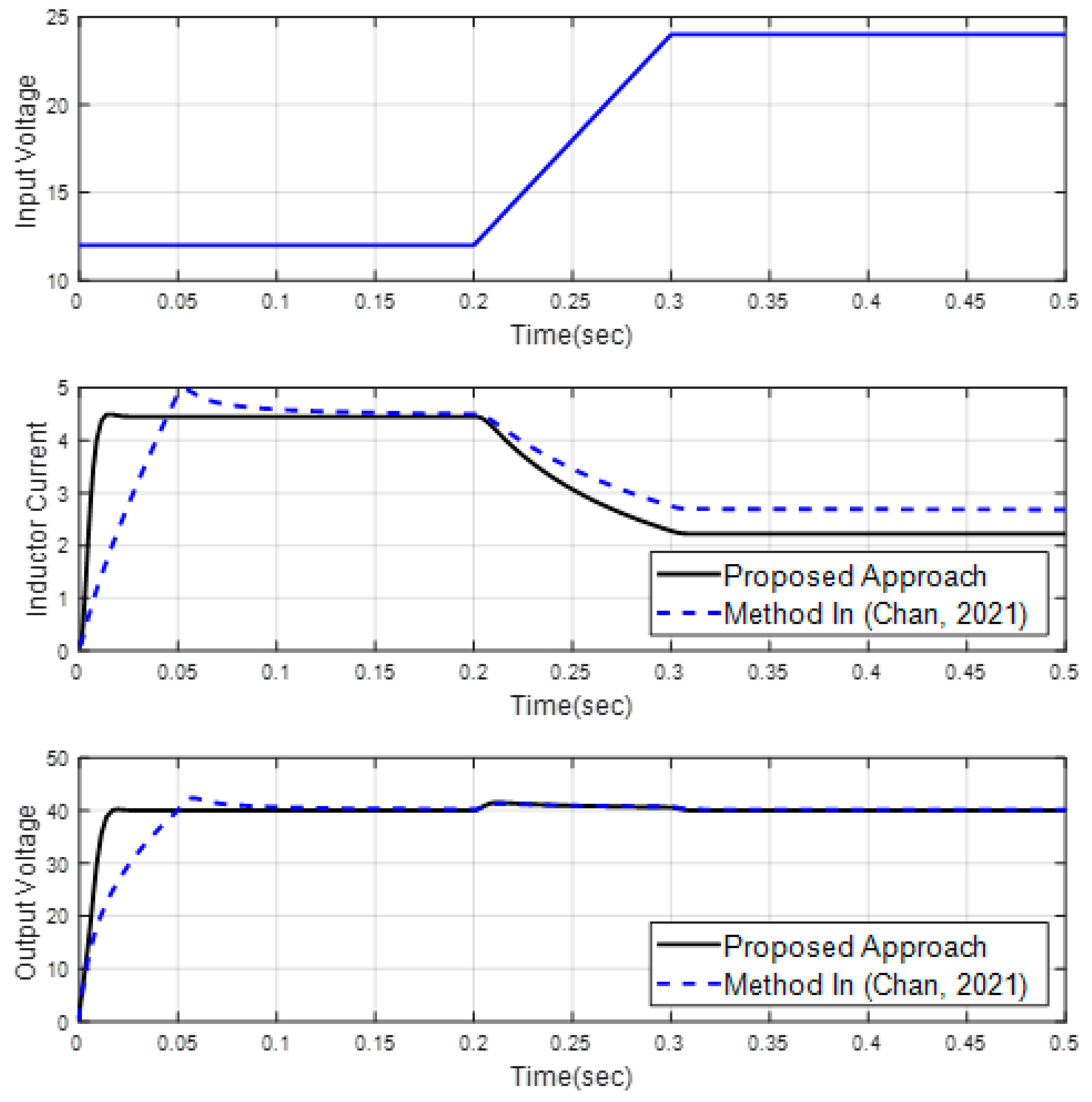
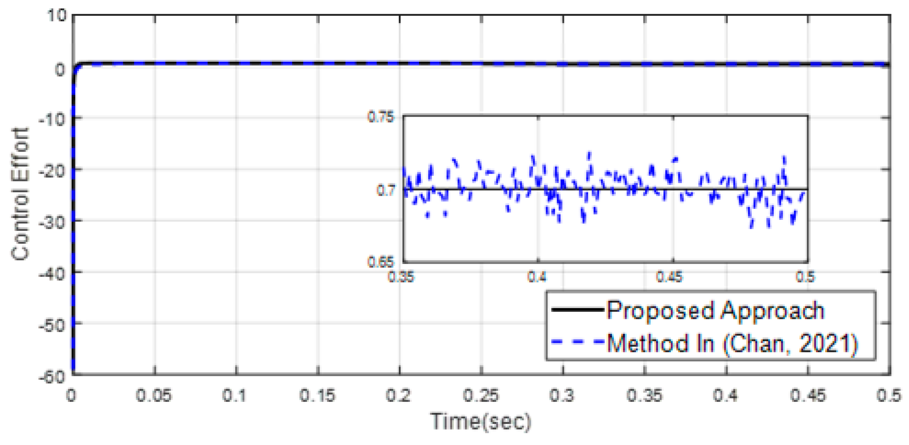
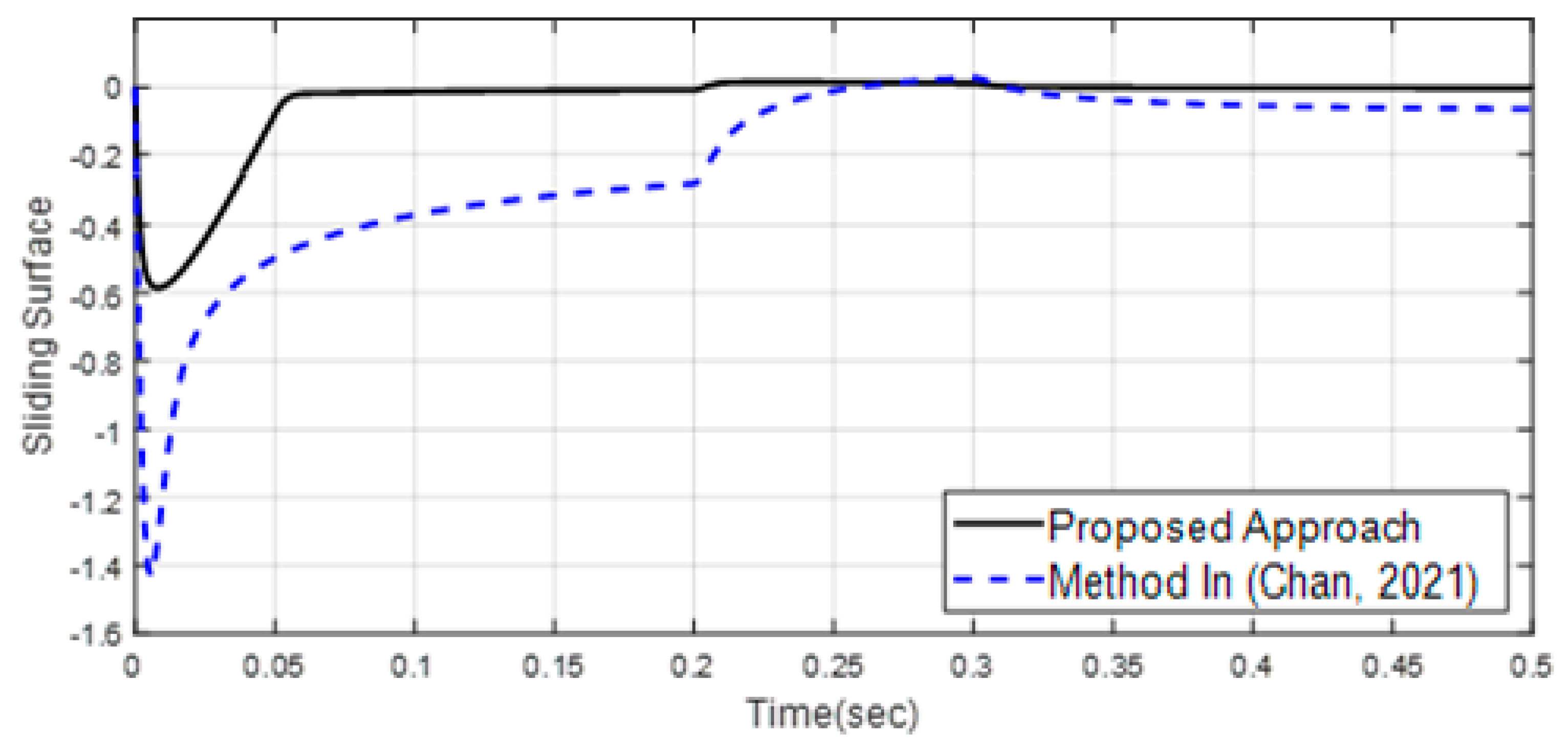
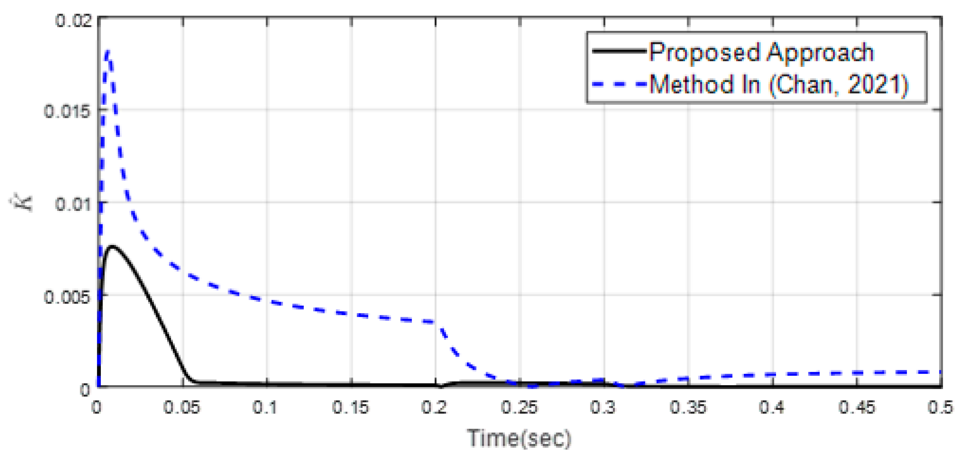
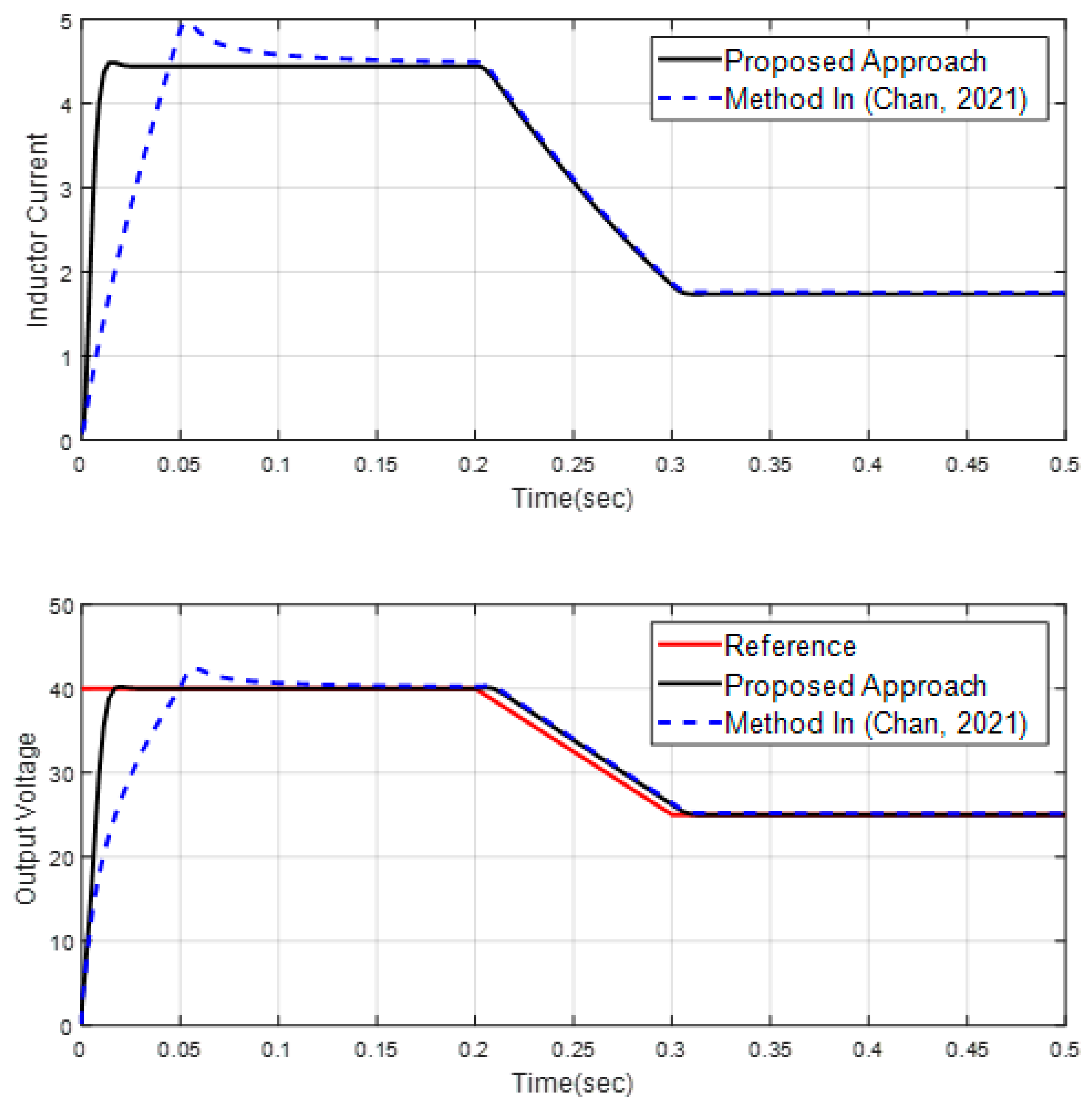
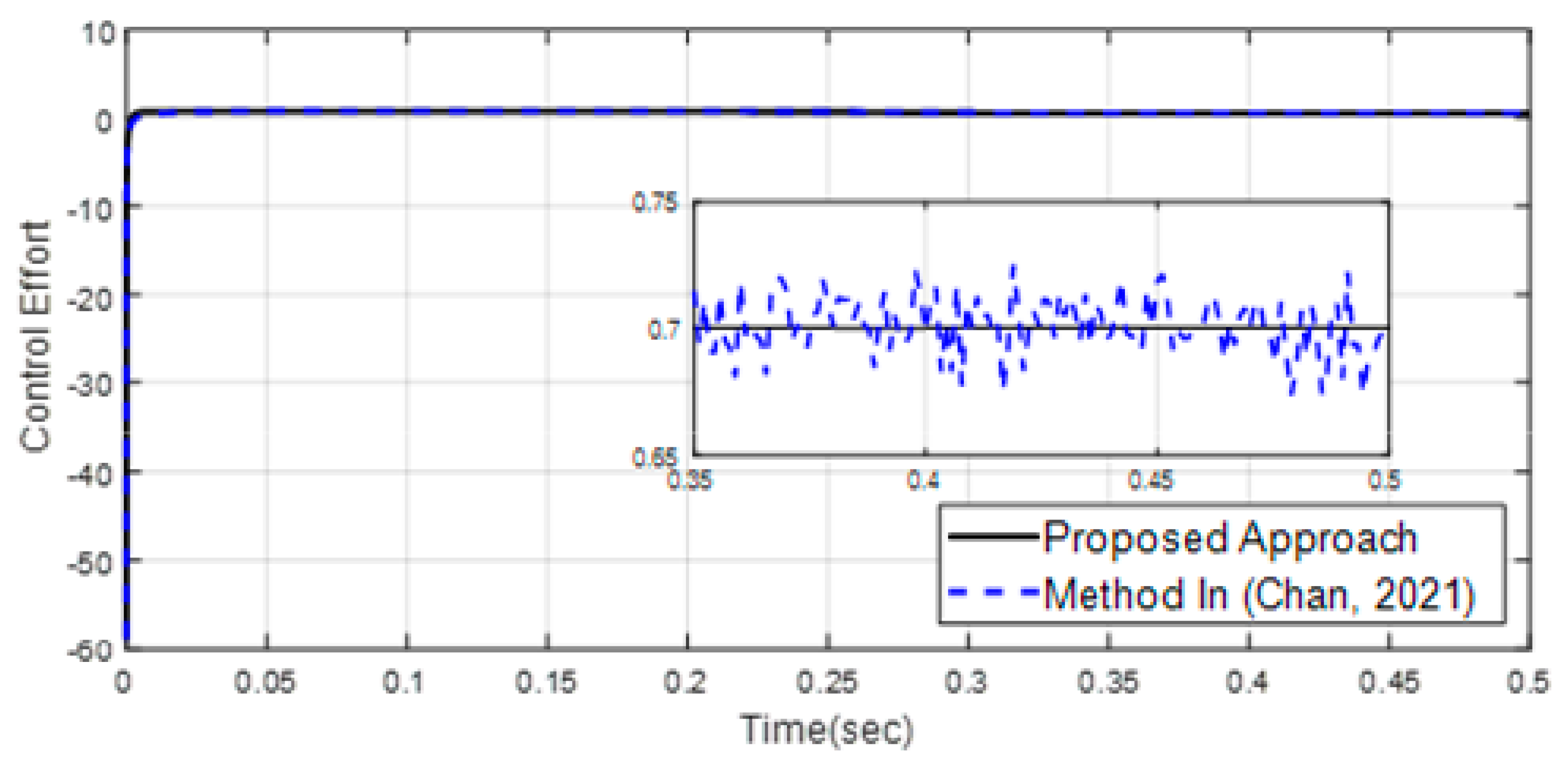
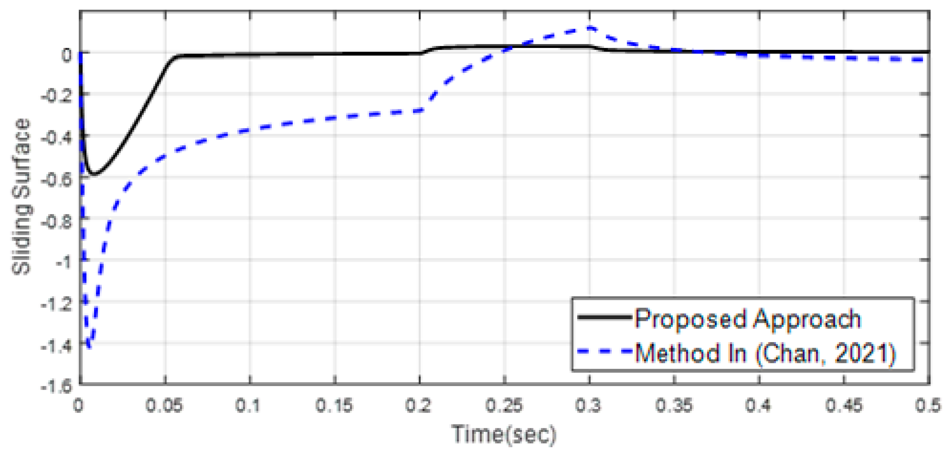
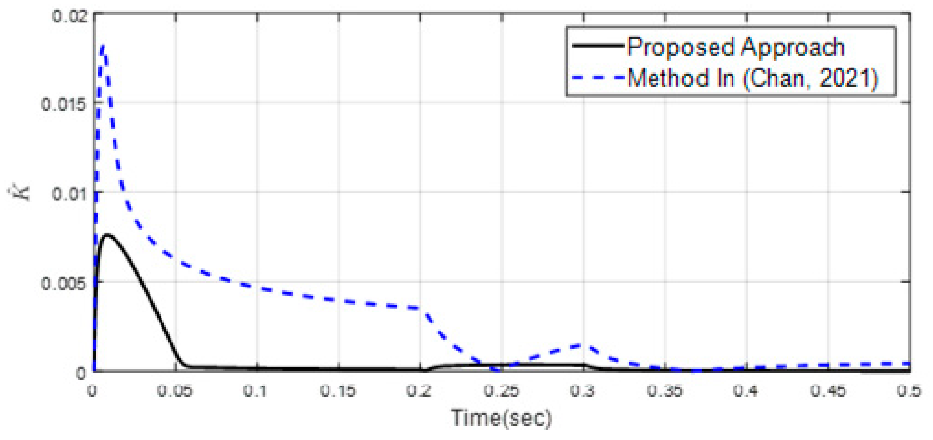
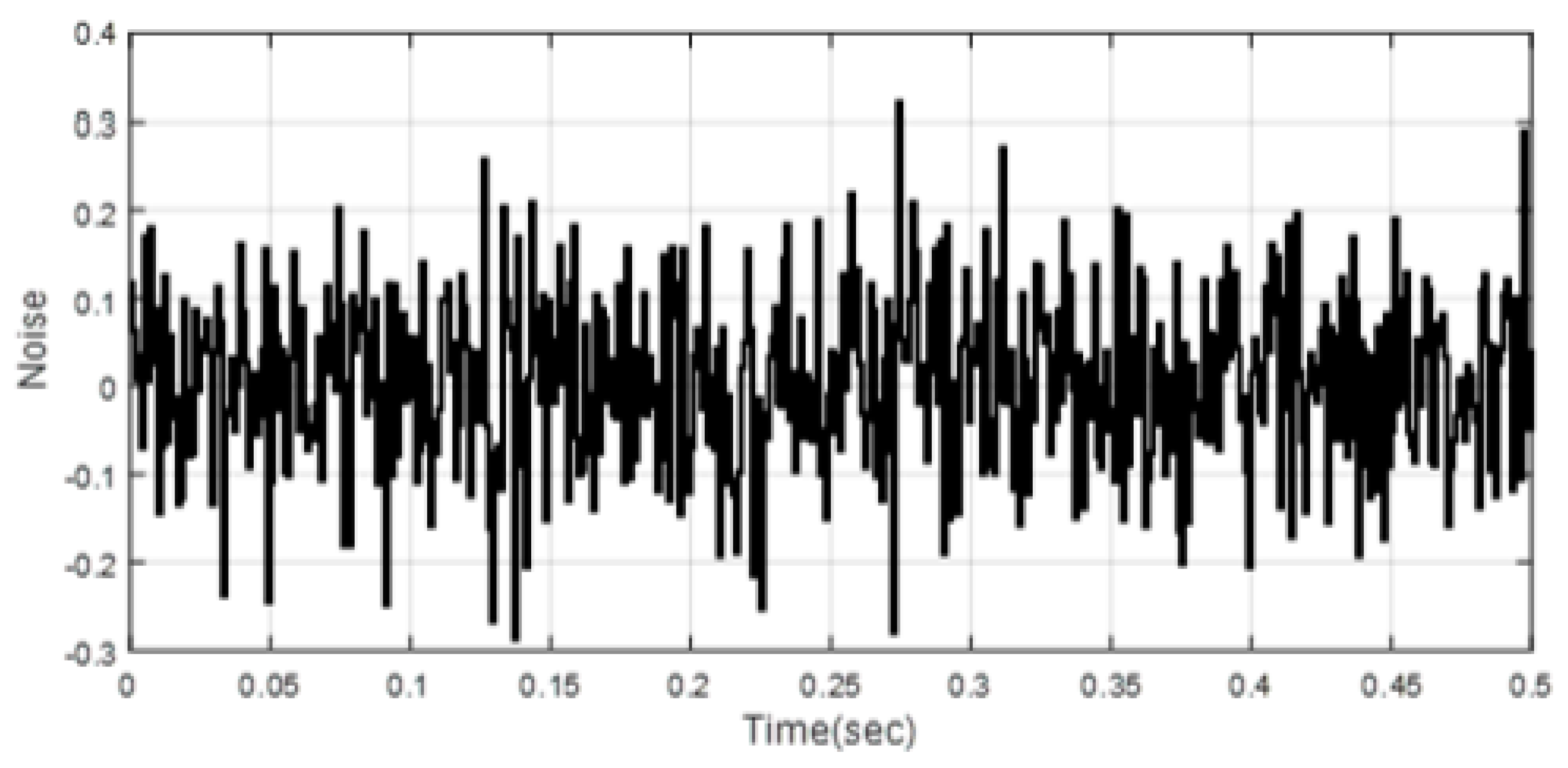
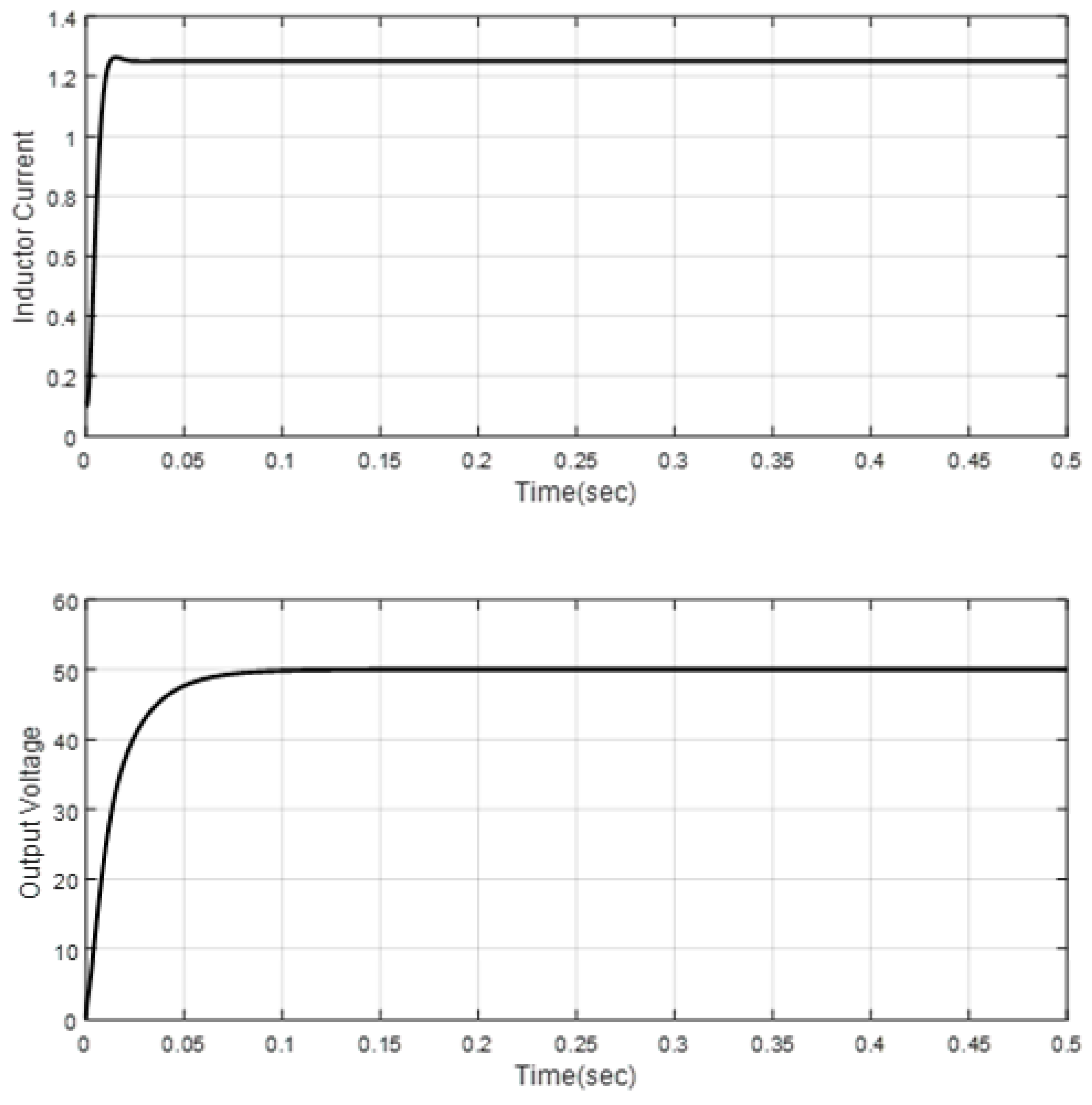
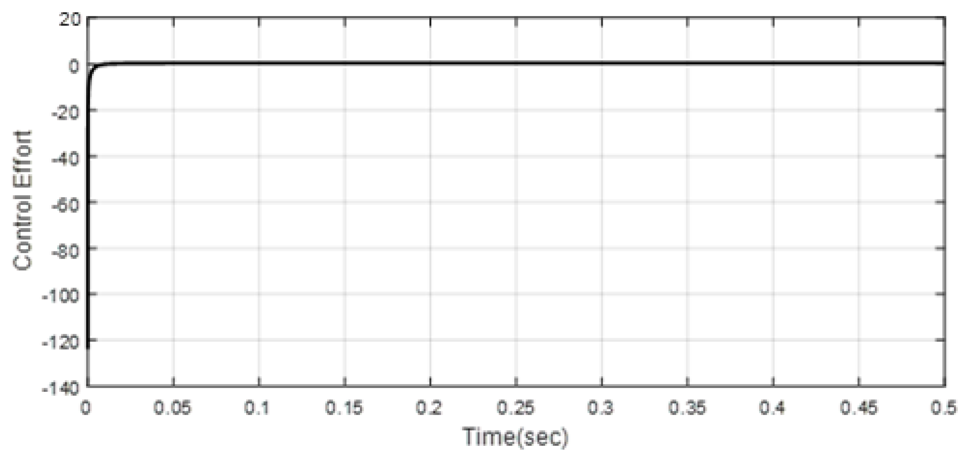
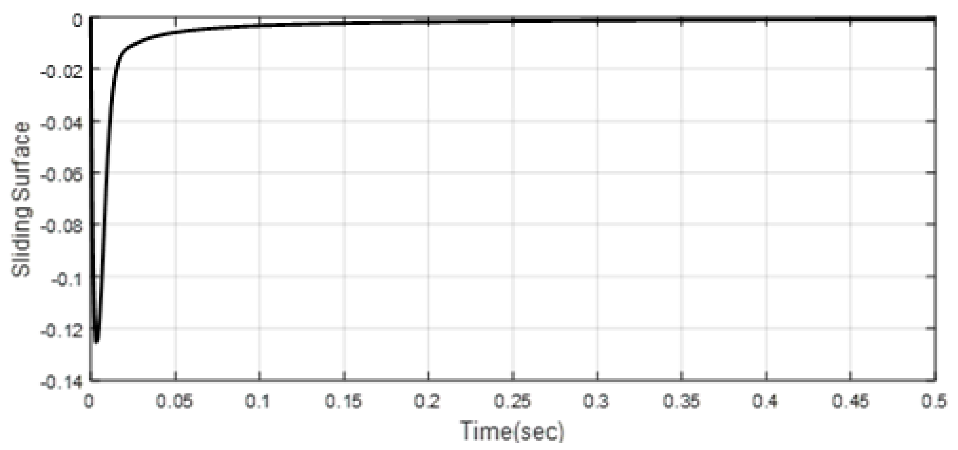
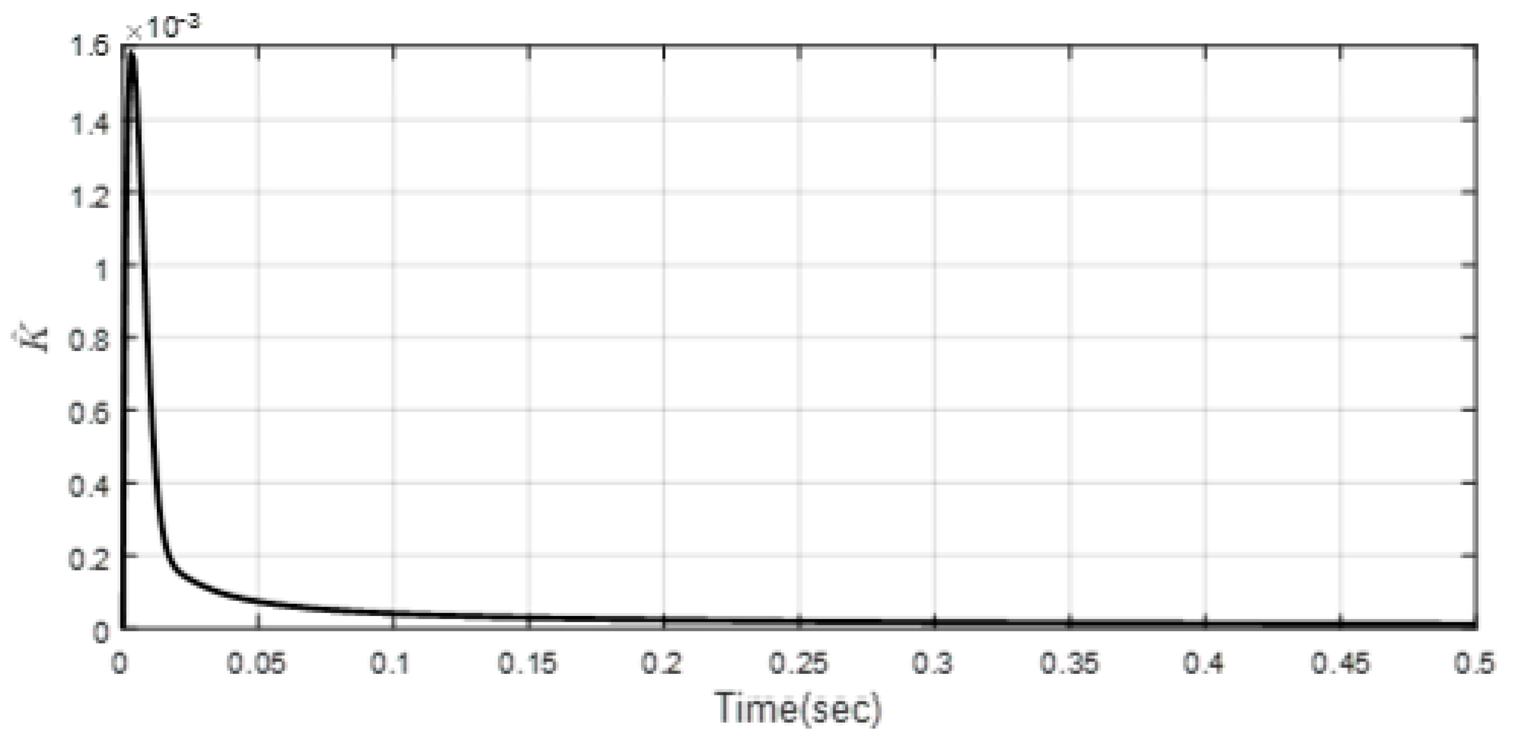
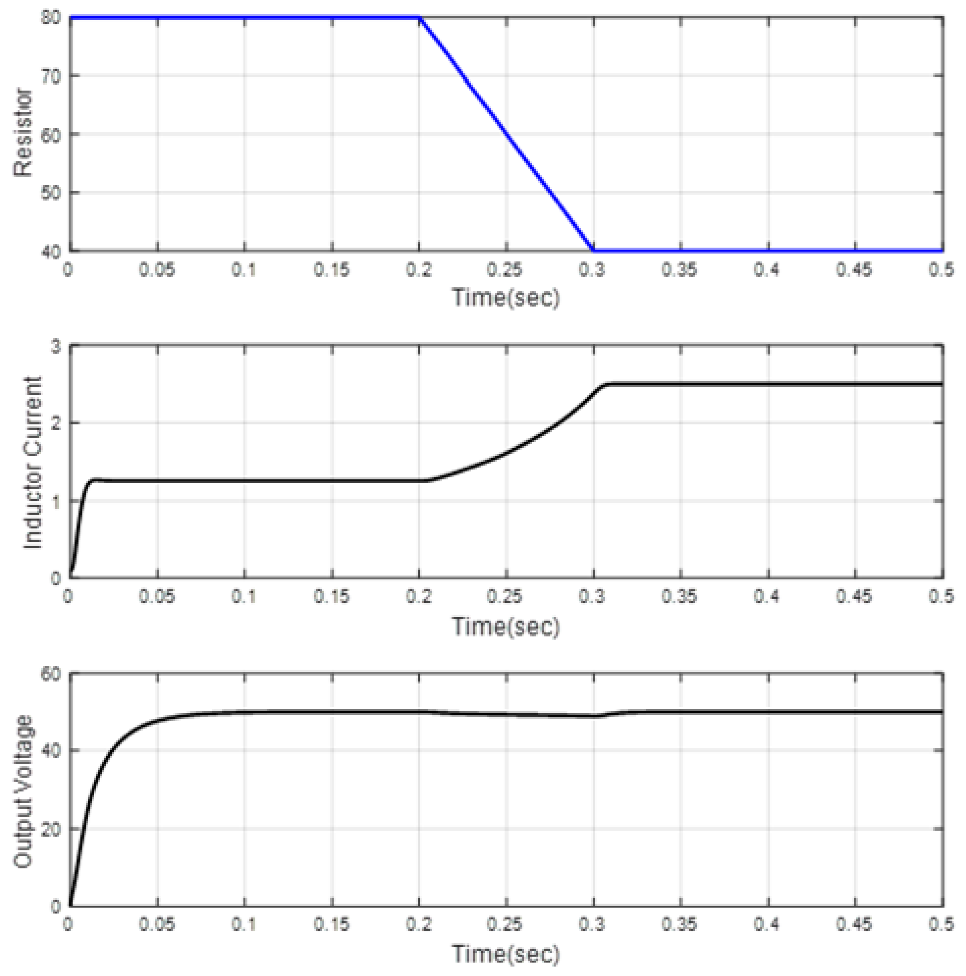
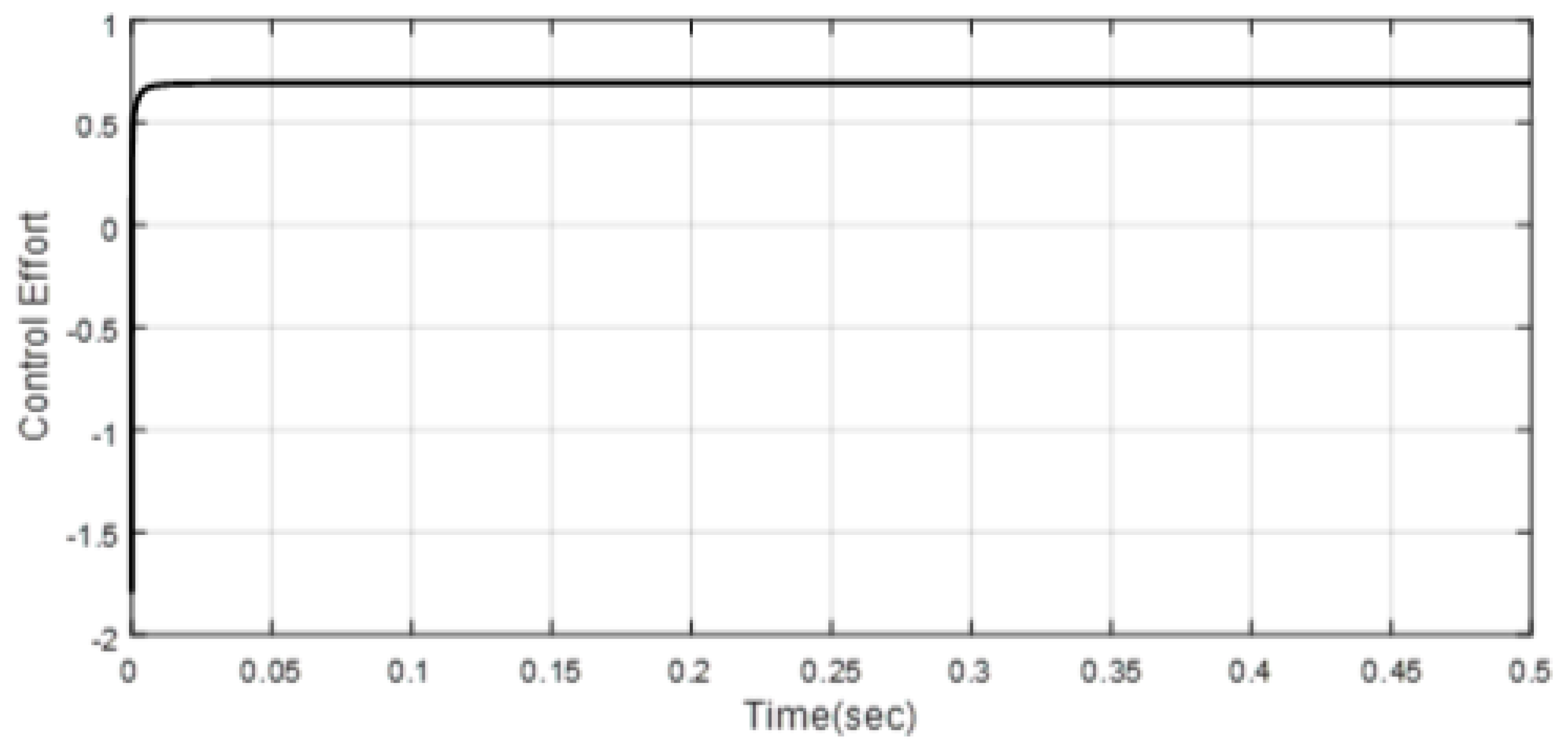
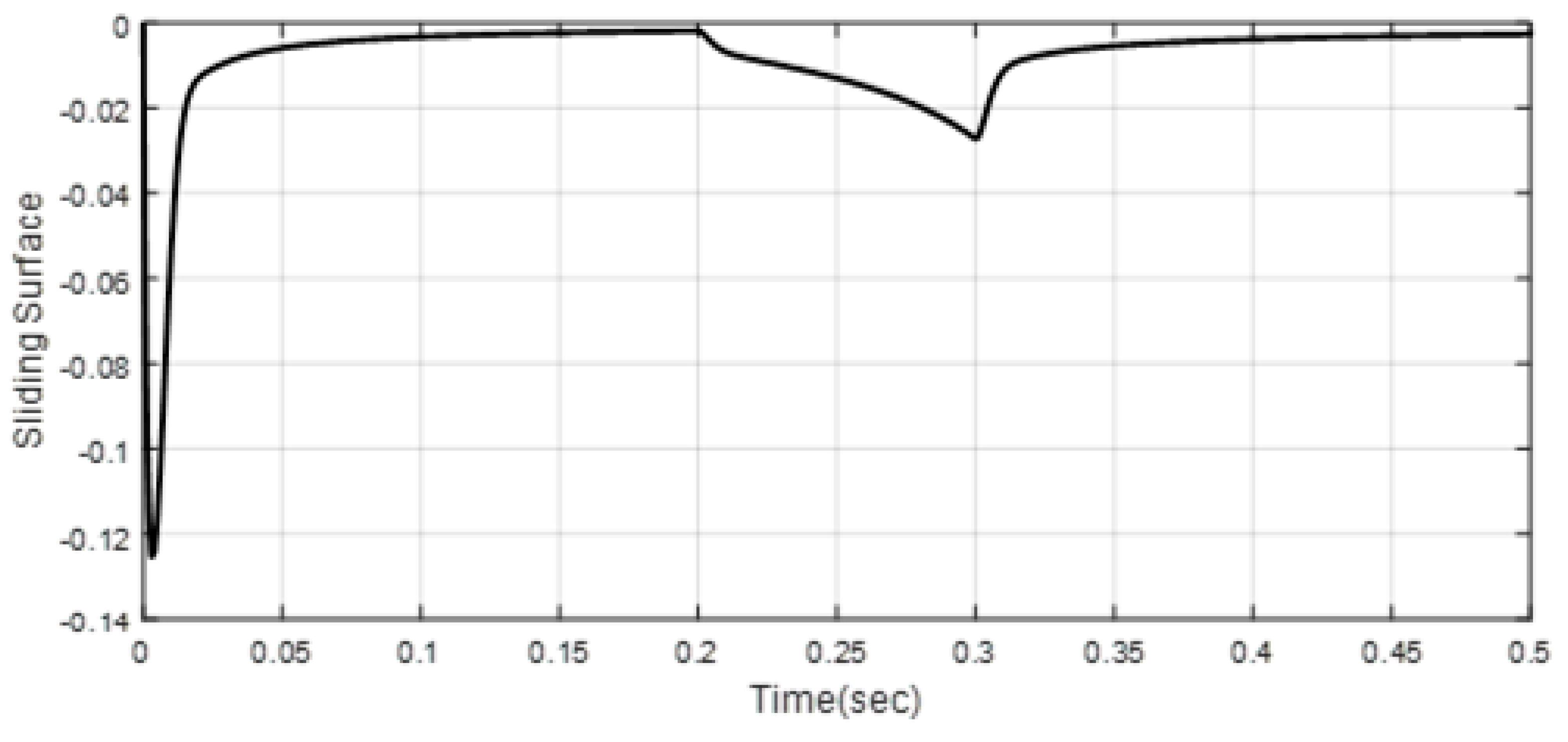
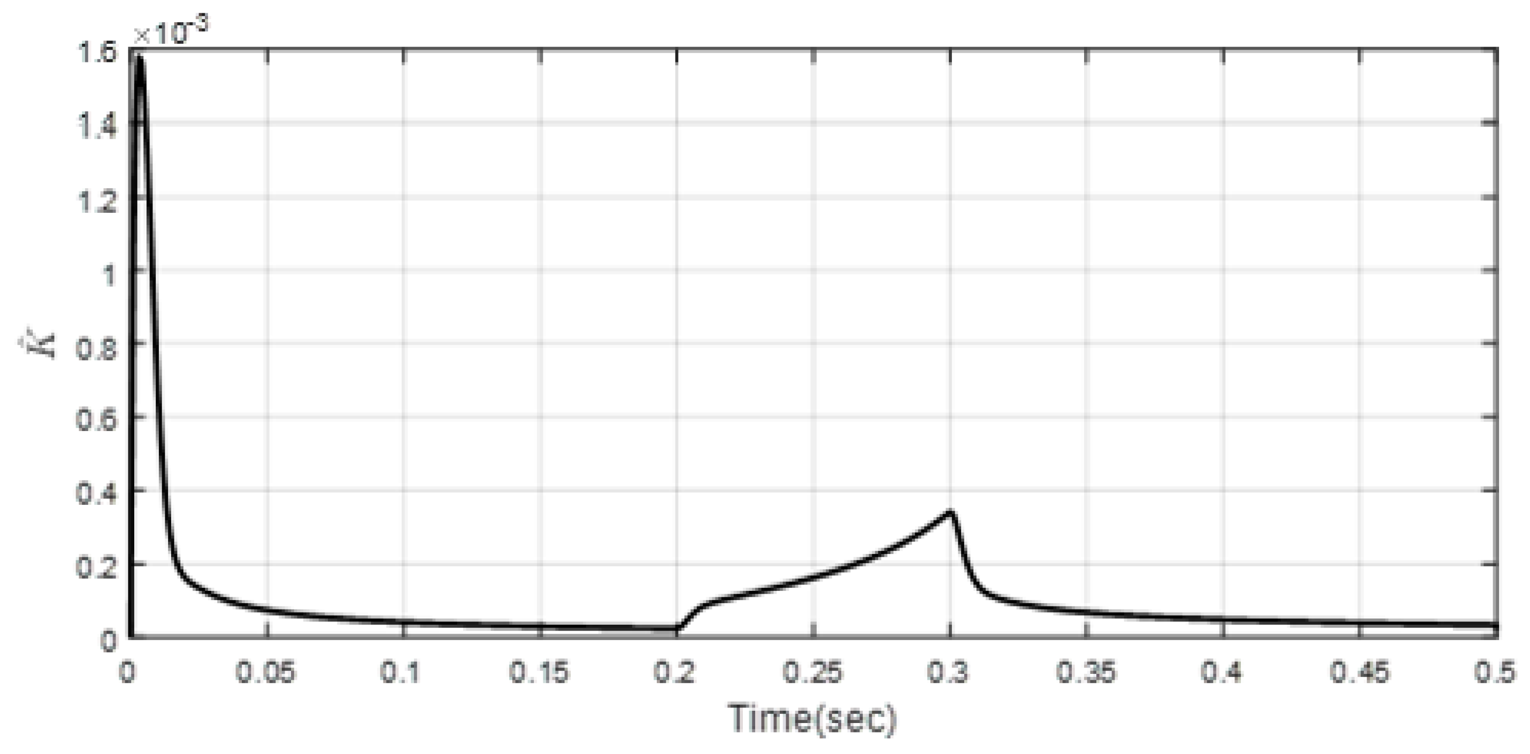
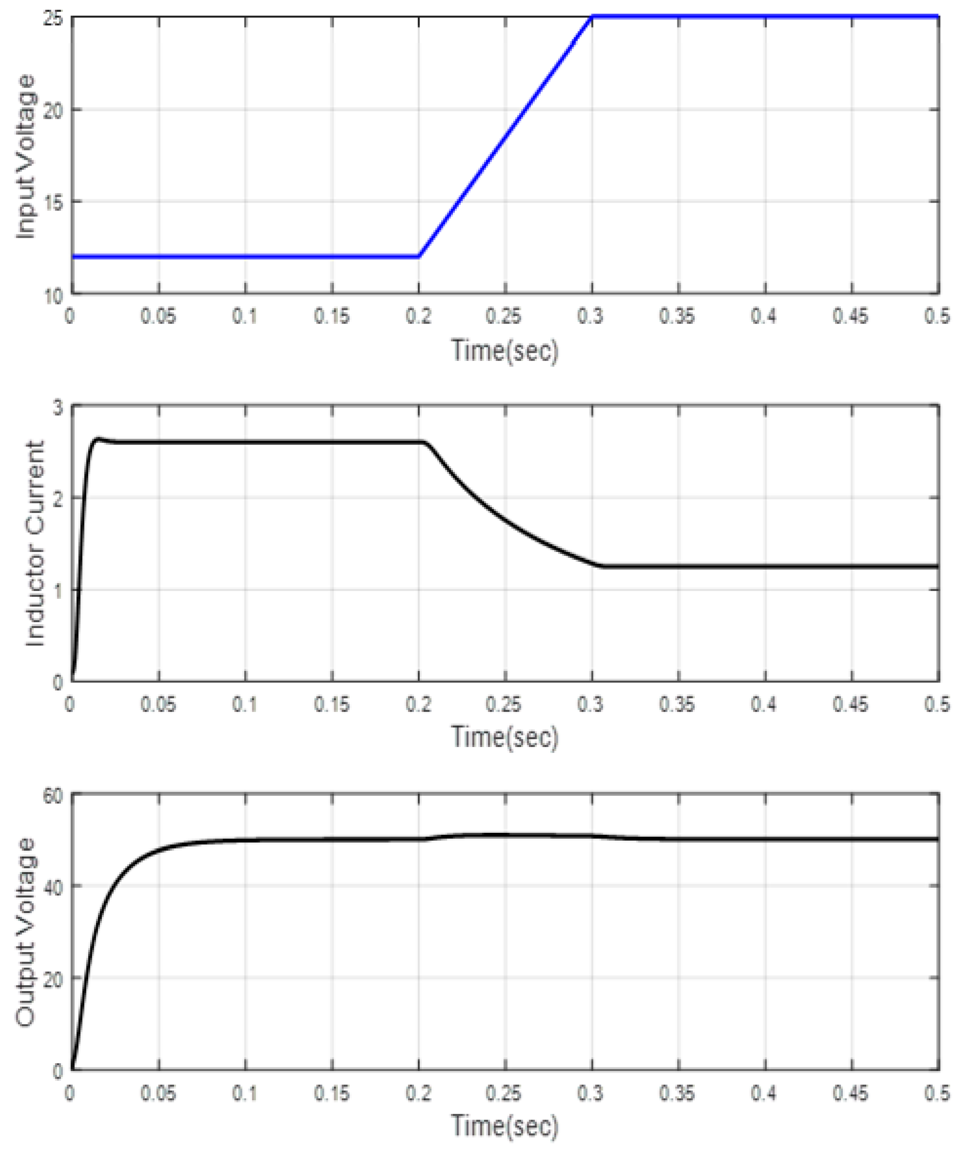
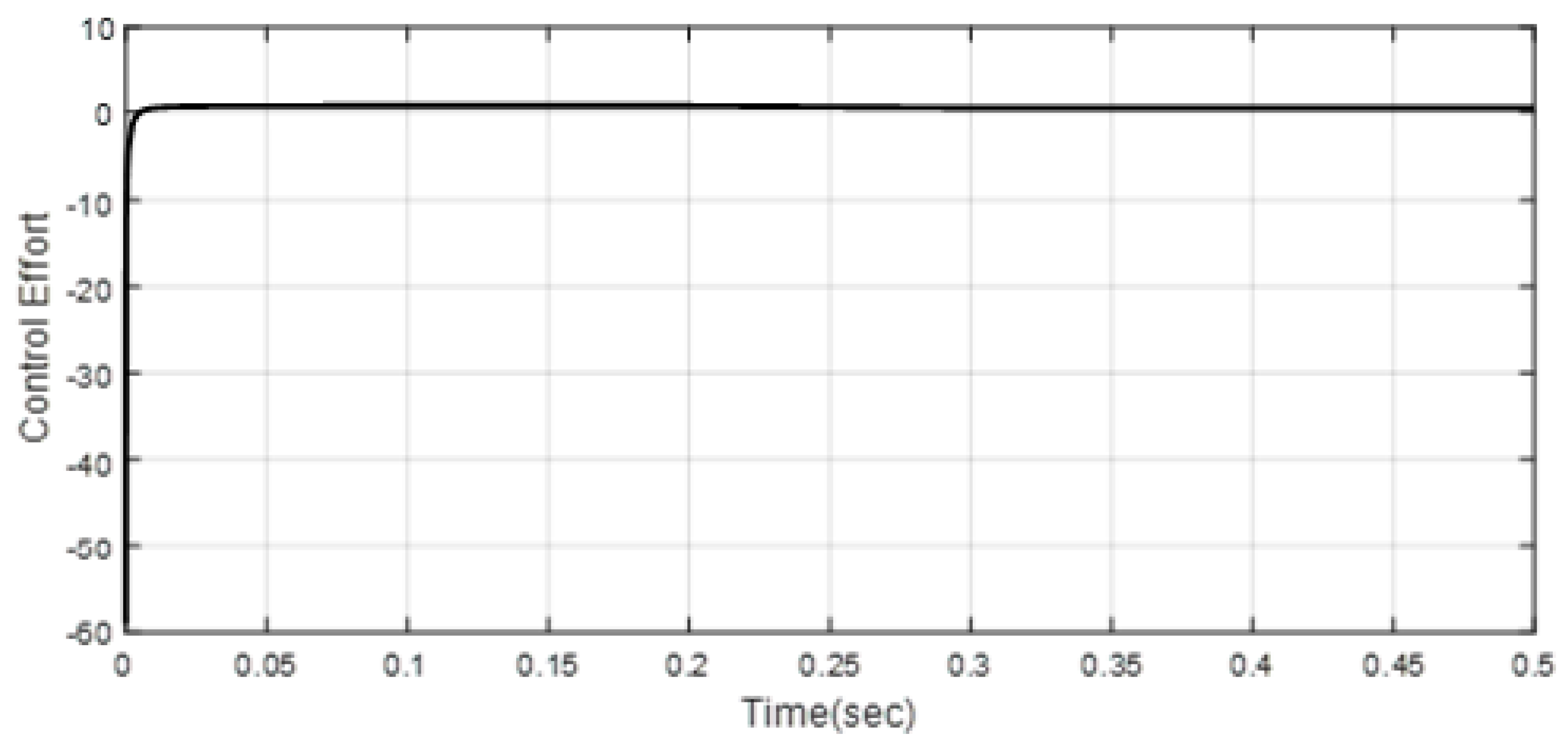
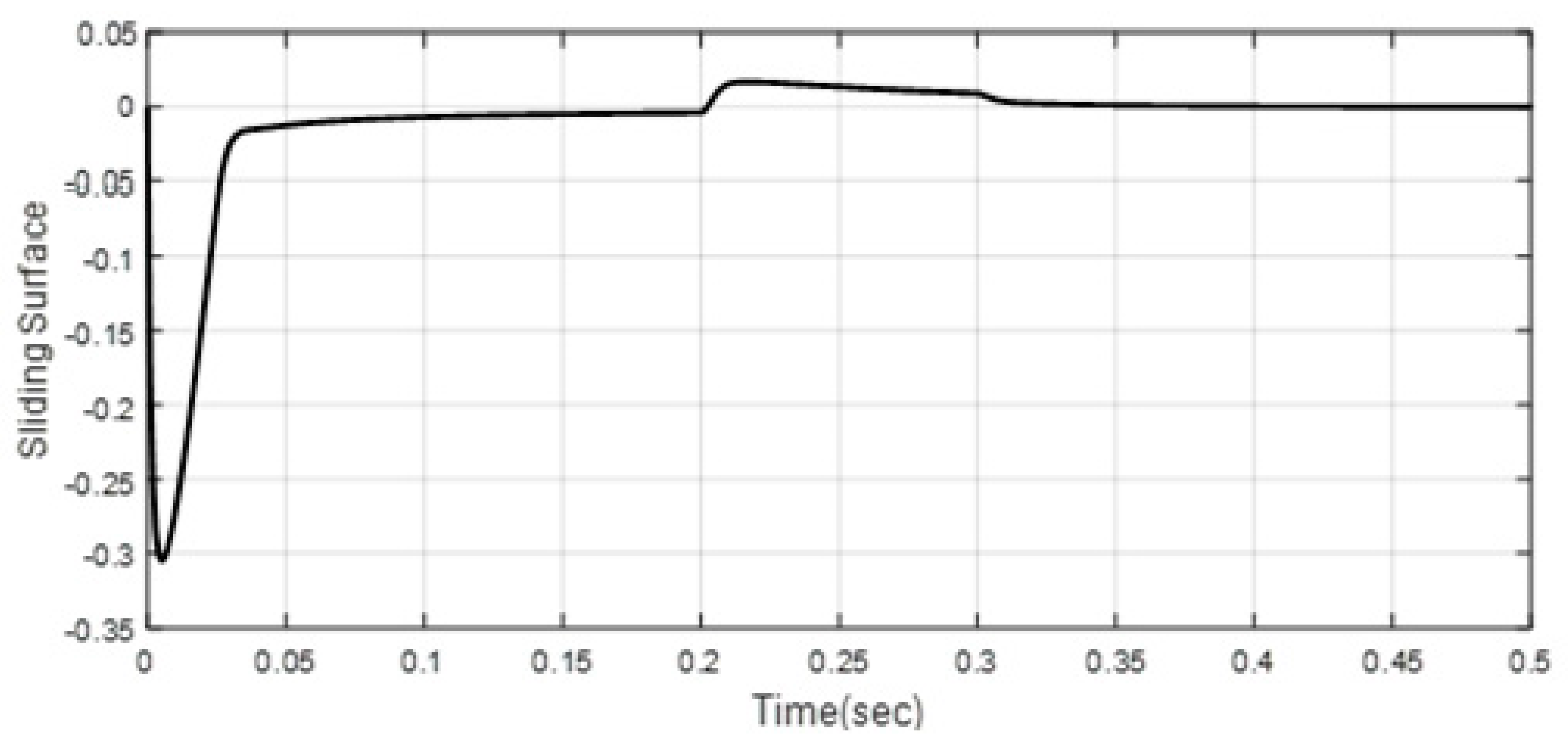
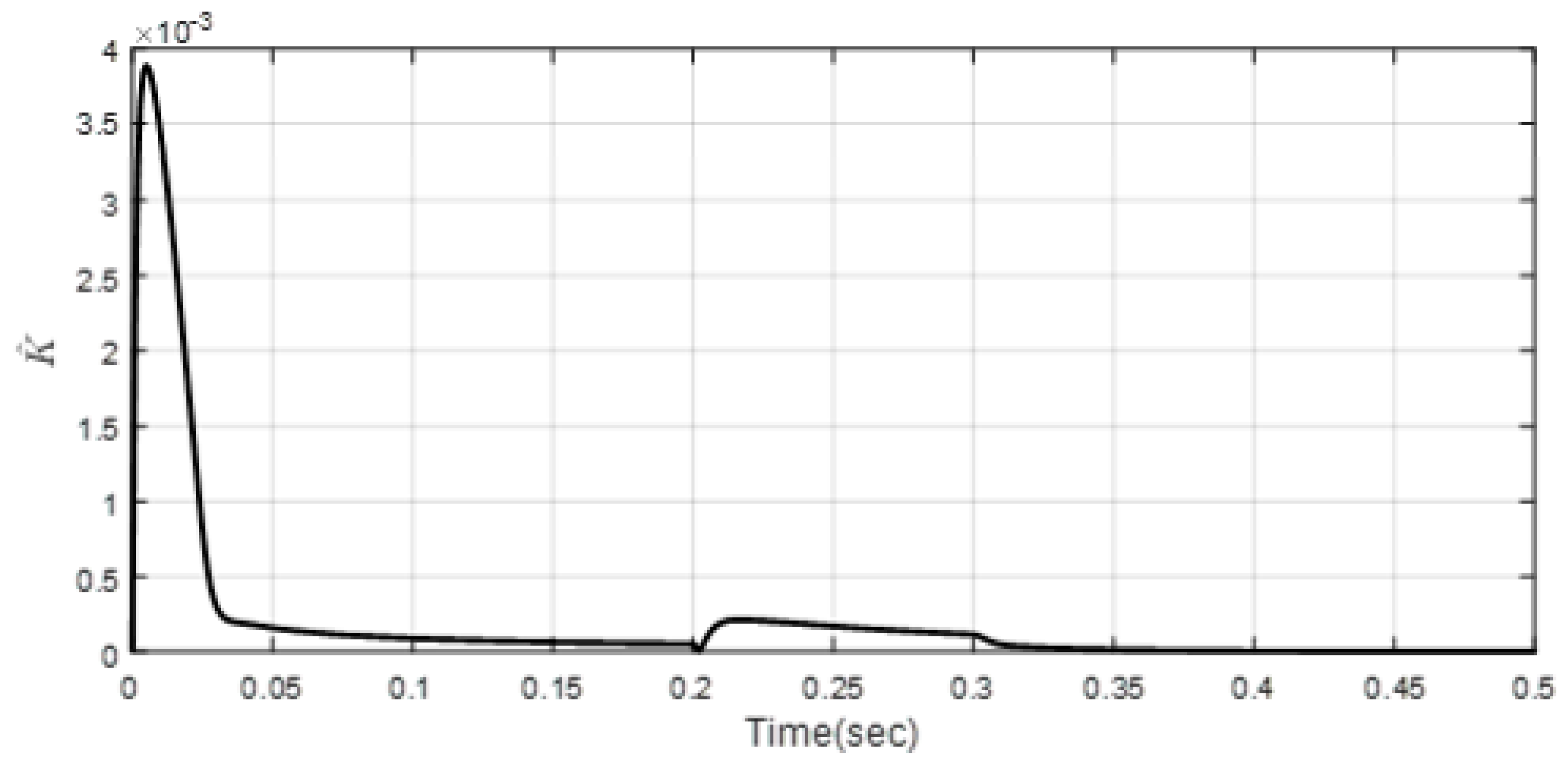
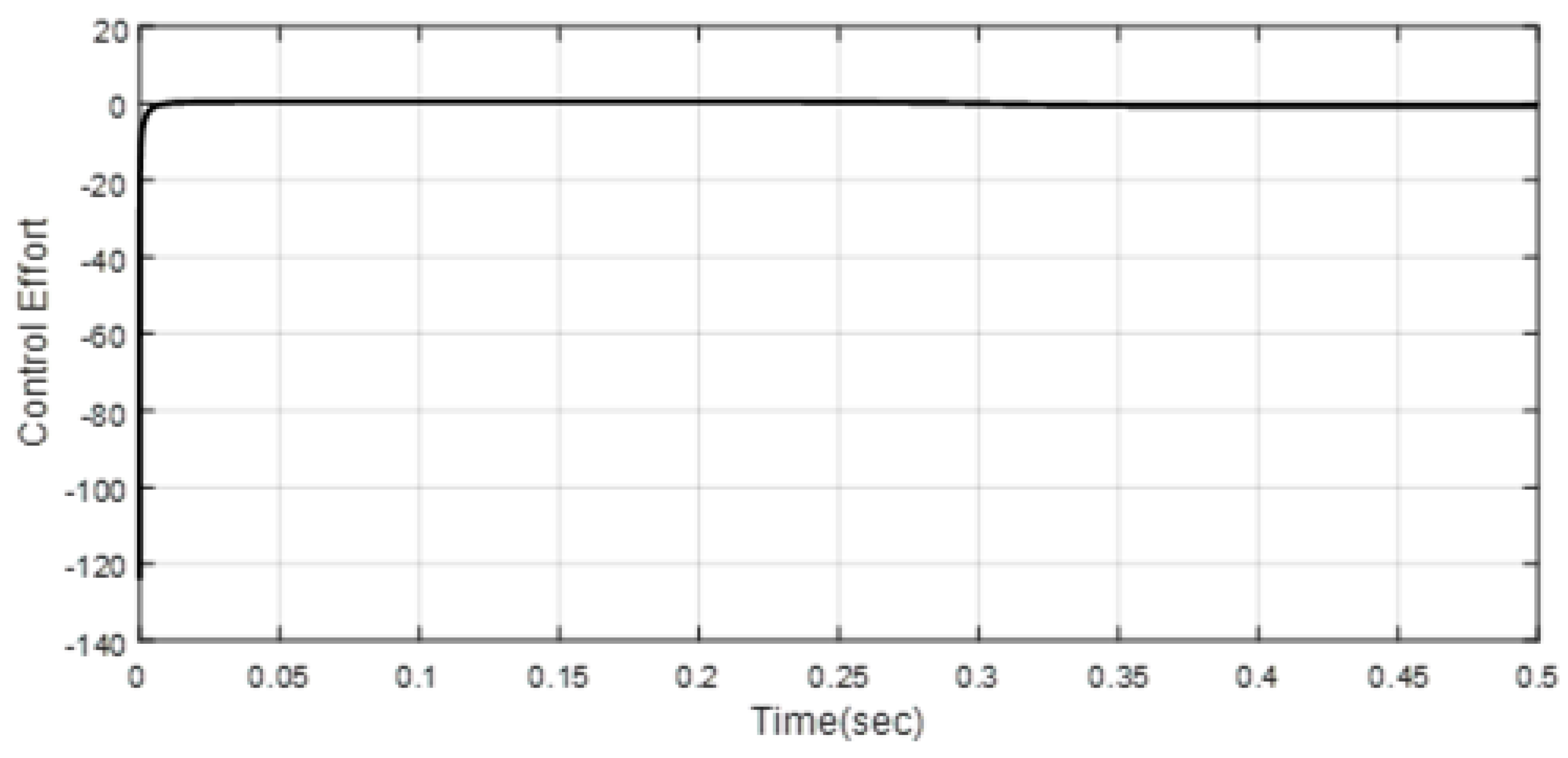
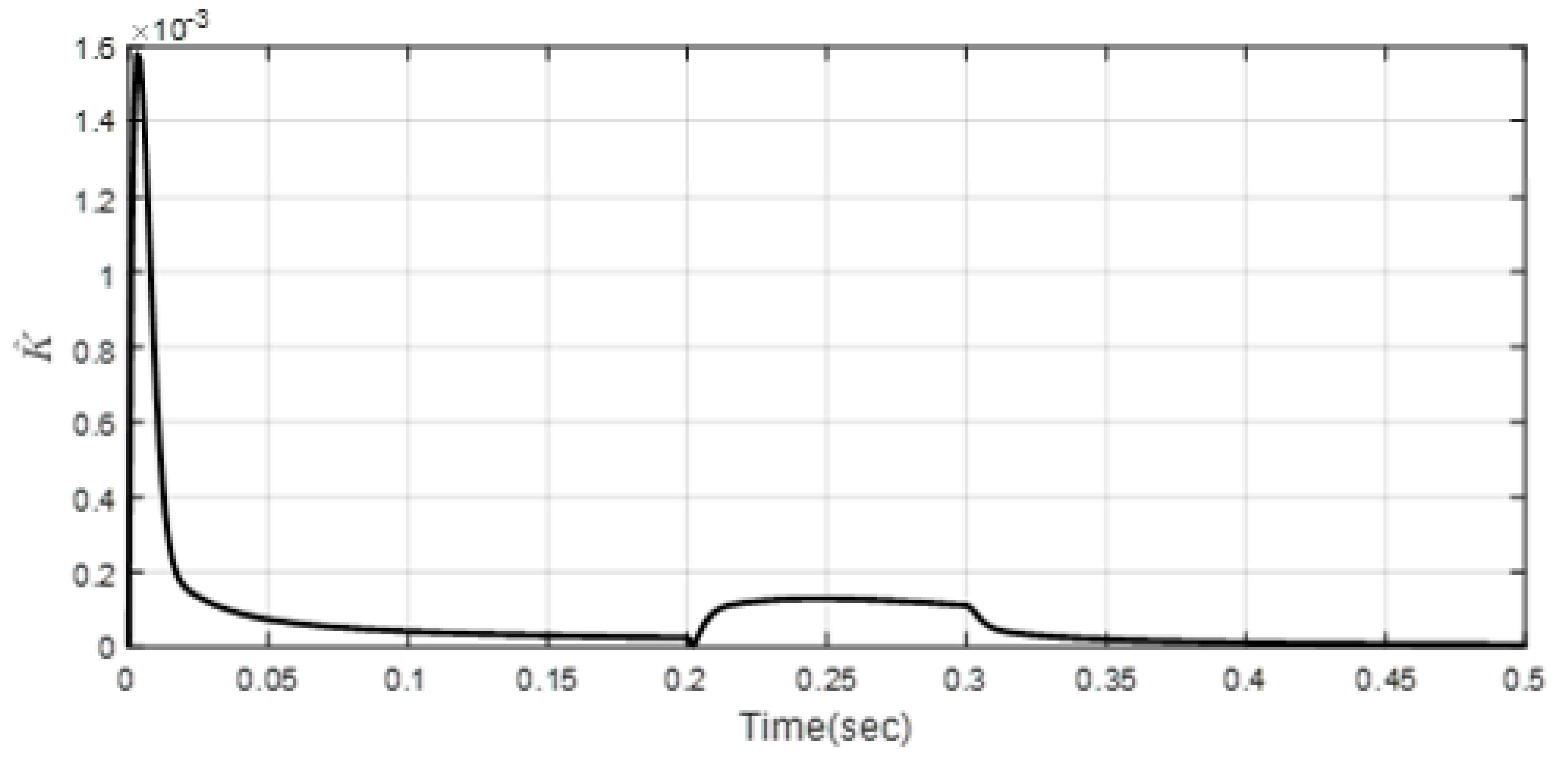
4. Simulation Results
5. Conclusions
Author Contributions
Funding
Institutional Review Board Statement
Informed Consent Statement
Data Availability Statement
Conflicts of Interest
Nomenclature
| Switch | Reference signal | ||
| Fast diode | Error signal | ||
| Resistance | Sliding surface | ||
| Inductor | Positive and constant parameter | ||
| Capacitor | Positive parameter | ||
| Control input | Positive parameter | ||
| Inductor current | Positive odd integer | ||
| Capacitor voltage | Positive odd integer with condition | ||
| Input voltage | Positive odd integer | ||
| Output voltage | The candidate Lyapunov’s function | ||
| Initial time | Positive constant | ||
| Settling time | Changes in the sliding surface | ||
| Converter state | Constant coefficient | ||
| External disturbances | Unknown upper bounds of external disturbances | ||
| Scalar value | Estimation of |
References
- Chan, C.-Y. Adaptive sliding-mode control of a novel buck-boost converter based on Zeta converter. IEEE Trans. Circuits Syst. II Express Briefs 2021, 69, 1307–1311. [Google Scholar] [CrossRef]
- Shen, L.; Lu, D.D.C.; Li, C. Adaptive sliding mode control method for DC–DC converters. IET Power Electron. 2015, 8, 1723–1732. [Google Scholar] [CrossRef]
- Hirsch, A.; Parag, Y.; Guerrero, J. Microgrids: A review of technologies, key drivers, and outstanding issues. Renew. Sustain. Energy Rev. 2018, 90, 402–411. [Google Scholar] [CrossRef]
- Lin, S.-Y.; Chen, J.-F. Distributed optimal power flow for smart grid transmission system with renewable energy sources. Energy 2013, 56, 184–192. [Google Scholar] [CrossRef]
- Sun, G.; Chen, S.; Wei, Z.; Chen, S. Multi-period integrated natural gas and electric power system probabilistic optimal power flow incorporating power-to-gas units. J. Mod. Power Syst. Clean Energy 2017, 5, 412–423. [Google Scholar] [CrossRef] [Green Version]
- Borlase, S. Smart Grids: Infrastructure, Technology, and Solutions; CRC Press: Boca Raton, FL, USA, 2017. [Google Scholar]
- Sinvula, R.; Abo-Al-Ez, K.M.; Kahn, M.T. Harmonic source detection methods: A systematic literature review. IEEE Access 2019, 7, 74283–74299. [Google Scholar] [CrossRef]
- Hatahet, W.; Marei, M.I.; Mokhtar, M. Adaptive controllers for grid-connected DC microgrids. Int. J. Electr. Power Energy Syst. 2021, 130, 106917. [Google Scholar] [CrossRef]
- Rana, N.; Banerjee, S. Development of an improved input-parallel output-series buck-boost converter and its closed-loop control. IEEE Trans. Ind. Electron. 2019, 67, 6428–6438. [Google Scholar] [CrossRef]
- Alajmi, B.N.; Marei, M.I.; Abdelsalam, I.; Ahmed, N.A. Multiphase Interleaved Converter Based on Cascaded Non-Inverting Buck-Boost Converter. IEEE Access 2022, 10, 42497–42506. [Google Scholar] [CrossRef]
- Zhang, Y.; Liu, H.; Li, J.; Sumner, M.; Xia, C. DC–DC boost converter with a wide input range and high voltage gain for fuel cell vehicles. IEEE Trans. Power Electron. 2018, 34, 4100–4111. [Google Scholar] [CrossRef]
- Özdemir, A.; Erdem, Z. Double-loop PI controller design of the DC-DC boost converter with a proposed approach for calculation of the controller parameters. Proc. Inst. Mech. Eng. Part I J. Syst. Control Eng. 2018, 232, 137–148. [Google Scholar] [CrossRef]
- Kobaku, T.; Jeyasenthil, R.; Sahoo, S.; Ramchand, R.; Dragicevic, T. Quantitative feedback design-based robust PID control of voltage mode controlled DC-DC boost converter. IEEE Trans. Circuits Syst. II Express Briefs 2020, 68, 286–290. [Google Scholar] [CrossRef]
- Yanarates, C.; Zhou, Z. Design and Cascade PI Controller-Based Robust Model Reference Adaptive Control of DC-DC Boost Converter. IEEE Access 2022, 10, 44909–44922. [Google Scholar] [CrossRef]
- Kazimierczuk, M.K.; Massarini, A. Feedforward control of DC-DC PWM boost converter. IEEE Trans. Circuits Syst. I Fundam. Theory Appl. 1997, 44, 143–148. [Google Scholar] [CrossRef]
- Chen, H.-C.; Lan, Y.-C. Unequal Duty-Ratio Feedforward Control to Extend Balanced-Currents Input Voltage Range for Series-Capacitor-Based Boost PFC Converter. IEEE Trans. Ind. Electron. 2022, 70, 4289–4292. [Google Scholar] [CrossRef]
- Adnan, M.F.; Oninda, M.A.M.; Nishat, M.M.; Islam, N. Design and simulation of a dc-dc boost converter with pid controller for enhanced performance. Int. J. Eng. Res. Technol. (IJERT) 2017, 6, 27–32. [Google Scholar]
- Ghazali, M.R.; Ahmad, M.A.; Suid, M.H.; Tumari, M.Z.M. A DC/DC Buck-Boost Converter-Inverter-DC Motor Control based on model-free PID Controller tuning by Adaptive Safe Experimentation Dynamics Algorithm. In Proceedings of the 2022 57th International Universities Power Engineering Conference (UPEC), Istanbul, Turkey, 30 August–2 September 2022; pp. 1–6. [Google Scholar]
- Karamanakos, P.; Geyer, T.; Manias, S. Direct voltage control of DC–DC boost converters using enumeration-based model predictive control. IEEE Trans. Power Electron. 2013, 29, 968–978. [Google Scholar] [CrossRef]
- Ullah, B.; Ullah, H.; Khalid, S. Direct Model Predictive Control of Noninverting Buck-boost DC-DC Converter. CES Trans. Electr. Mach. Syst. 2022, 6, 332–339. [Google Scholar] [CrossRef]
- Gupta, T.; Boudreaux, R.; Nelms, R.M.; Hung, J.Y. Implementation of a fuzzy controller for DC-DC converters using an inexpensive 8-b microcontroller. IEEE Trans. Ind. Electron. 1997, 44, 661–669. [Google Scholar] [CrossRef]
- So, W.-C.; Tse, C.K.; Lee, Y.-S. A fuzzy controller for DC-DC converters. In Proceedings of the 1994 Power Electronics Specialist Conference-PESC’94, Taipei, Taiwan, 20–25 June 1994; pp. 315–320. [Google Scholar]
- Beccuti, A.G.; Papafotiou, G.; Morari, M. Optimal control of the boost dc-dc converter. In Proceedings of the 44th IEEE Conference on Decision and Control, Seville, Spain, 12–15 December 2005; pp. 4457–4462. [Google Scholar]
- Mitra, L.; Rout, U.K. Optimal control of a high gain DC-DC converter. Int. J. Power Electron. Drive Syst. 2022, 13, 256. [Google Scholar] [CrossRef]
- Kahani, R.; Jamil, M.; Iqbal, M.T. Direct Model Reference Adaptive Control of a Boost Converter for Voltage Regulation in Microgrids. Energies 2022, 15, 5080. [Google Scholar] [CrossRef]
- Jeong, G.-J.; Kim, I.-H.; Son, Y.-I. Application of simple adaptive control to a dc/dc boost converter with load variation. In Proceedings of the 2009 ICCAS-SICE, Fukuoka, Japan, 18–21 August 2009; pp. 1747–1751. [Google Scholar]
- Guldemir, H. Sliding mode control of DC-DC boost converter. J. Appl. Sci. 2005, 5, 588–592. [Google Scholar] [CrossRef] [Green Version]
- Utkin, V. Sliding mode control of DC/DC converters. J. Frankl. Inst. 2013, 350, 2146–2165. [Google Scholar] [CrossRef] [Green Version]
- Wang, J.; Rong, J.; Yu, L. Dynamic prescribed performance sliding mode control for DC–DC buck converter system with mismatched time-varying disturbances. ISA Trans. 2022, 129, 546–557. [Google Scholar] [CrossRef]
- Wai, R.-J.; Shih, L.-C. Adaptive fuzzy-neural-network design for voltage tracking control of a DC–DC boost converter. IEEE Trans. Power Electron. 2011, 27, 2104–2115. [Google Scholar] [CrossRef]
- Wang, Y.-X.; Yu, D.-H.; Kim, Y.-B. Robust time-delay control for the DC–DC boost converter. IEEE Trans. Ind. Electron. 2013, 61, 4829–4837. [Google Scholar] [CrossRef]
- Rojsiraphisal, T.; Mobayen, S.; Asad, J.H.; Vu, M.T.; Chang, A.; Puangmalai, J. Fast terminal sliding control of underactuated robotic systems based on disturbance observer with experimental validation. Mathematics 2021, 9, 1935. [Google Scholar] [CrossRef]
- Ghadiri, H.; Khodadadi, H.; Mobayen, S.; Asad, J.H.; Rojsiraphisal, T.; Chang, A. Observer-based robust control method for switched neutral systems in the presence of interval time-varying delays. Mathematics 2021, 9, 2473. [Google Scholar] [CrossRef]
- Sarkar, T.T.; Mahanta, C. Estimation Based Sliding Mode Control of DC-DC Boost Converters. IFAC-PapersOnLine 2022, 55, 467–472. [Google Scholar] [CrossRef]
- Sepestanaki, M.A.; Jalilvand, A.; Mobayen, S.; Zhang, C. Design of adaptive continuous barrier function finite time stabilizer for TLP systems in floating offshore wind turbines. Ocean Eng. 2022, 262, 112267. [Google Scholar] [CrossRef]
- Utkin, V. Discussion aspects of high-order sliding mode control. IEEE Trans. Autom. Control 2015, 61, 829–833. [Google Scholar] [CrossRef]
- Liu, X.; Han, Y.; Wang, C. Second-order sliding mode control for power optimisation of DFIG-based variable speed wind turbine. IET Renew. Power Gener. 2017, 11, 408–418. [Google Scholar] [CrossRef]
- Liu, X.; Han, Y. Decentralized multi-machine power system excitation control using continuous higher-order sliding mode technique. Int. J. Electr. Power Energy Syst. 2016, 82, 76–86. [Google Scholar] [CrossRef]
- RakhtAla, S.M.; Yasoubi, M.; HosseinNia, H. Design of second order sliding mode and sliding mode algorithms: A practical insight to DC-DC buck converter. IEEE/CAA J. Autom. Sin. 2017, 4, 483–497. [Google Scholar] [CrossRef] [Green Version]
- Ma, R.; Wu, Y.; Breaz, E.; Huangfu, Y.; Briois, P.; Gao, F. High-order sliding mode control of DC-DC converter for PEM fuel cell applications. In Proceedings of the 2018 IEEE Industry Applications Society Annual Meeting (IAS), Portland, OR, USA, 23–27 September 2018; pp. 1–7. [Google Scholar]
- Xiu, C.; Guo, P. Global terminal sliding mode control with the quick reaching law and its application. IEEE Access 2018, 6, 49793–49800. [Google Scholar] [CrossRef]
- Ahmed, S.; Wang, H.; Tian, Y. Adaptive fractional high-order terminal sliding mode control for nonlinear robotic manipulator under alternating loads. Asian J. Control 2021, 23, 1900–1910. [Google Scholar] [CrossRef]
- Yang, L.; Yang, J. Robust finite-time convergence of chaotic systems via adaptive terminal sliding mode scheme. Commun. Nonlinear Sci. Numer. Simul. 2011, 16, 2405–2413. [Google Scholar] [CrossRef]
- Yao, Q. Fixed-time trajectory tracking control for unmanned surface vessels in the presence of model uncertainties and external disturbances. Int. J. Control 2022, 95, 1133–1143. [Google Scholar] [CrossRef]
- Aghababa, M.P. Finite-time chaos control and synchronization of fractional-order nonautonomous chaotic (hyperchaotic) systems using fractional nonsingular terminal sliding mode technique. Nonlinear Dyn. 2012, 69, 247–261. [Google Scholar] [CrossRef]


| Scenario 1 | ||||||
|---|---|---|---|---|---|---|
| Proposed Approach | The Method in Ref. [1] | |||||
| Converge time | 0.022 | 0.0194 | 0.0195 | 0.113 | 0.0817 | 0.153 |
| Overshoot | 0.031 | 0 | 0 | 0.33 | 1.87 | 0.01 |
| Undershoot | 0 | 0 | 0 | 0 | 0 | 0 |
| Chattering | NO | NO | NO | NO | NO | YES |
| Scenario 2 | ||||||
|---|---|---|---|---|---|---|
| Proposed Approach | The Method in Ref. [1] | |||||
| Converge time | 0.0137 | 0.0195 | 0.0116 | 0.05299 | 0.0672 | 0.02213 |
| Overshoot | 0 | 0 | 0 | 0.157 | 1.47 | 0 |
| Undershoot | 0 | 1 | 0 | 0 | 1 | 0 |
| Chattering | NO | NO | NO | NO | NO | YES |
| Scenario 3 | ||||||
|---|---|---|---|---|---|---|
| Proposed Approach | The method in Ref. [1] | |||||
| Converge time | 0.02213 | 0.1787 | 0.0087 | 0.1302 | 0.09635 | 0.333 |
| Overshoot | 0.042 | 1.28 | 0 | 0.522 | 2.41 | 0 |
| Undershoot | 0 | 0 | 0 | 0 | 0 | 0 |
| Chattering | NO | NO | NO | NO | NO | YES |
| Scenario 4 | ||||||
|---|---|---|---|---|---|---|
| Proposed Approach | The method in Ref. [1] | |||||
| Converge time | 0.02774 | 0.02511 | 0.0056 | 0.1321 | 0.113 | 0.02956 |
| Overshoot | 0.026 | 0.24 | 0 | 0. 511 | 2.41 | 0 |
| Undershoot | 0 | 0 | 0 | 0 | 0 | 0 |
| Chattering | NO | NO | NO | NO | NO | YES |
Disclaimer/Publisher’s Note: The statements, opinions and data contained in all publications are solely those of the individual author(s) and contributor(s) and not of MDPI and/or the editor(s). MDPI and/or the editor(s) disclaim responsibility for any injury to people or property resulting from any ideas, methods, instructions or products referred to in the content. |
© 2023 by the authors. Licensee MDPI, Basel, Switzerland. This article is an open access article distributed under the terms and conditions of the Creative Commons Attribution (CC BY) license (https://creativecommons.org/licenses/by/4.0/).
Share and Cite
Alnuman, H.; Hsia, K.-H.; Sepestanaki, M.A.; Ahmed, E.M.; Mobayen, S.; Armghan, A. Design of Continuous Finite-Time Controller Based on Adaptive Tuning Approach for Disturbed Boost Converters. Mathematics 2023, 11, 1757. https://doi.org/10.3390/math11071757
Alnuman H, Hsia K-H, Sepestanaki MA, Ahmed EM, Mobayen S, Armghan A. Design of Continuous Finite-Time Controller Based on Adaptive Tuning Approach for Disturbed Boost Converters. Mathematics. 2023; 11(7):1757. https://doi.org/10.3390/math11071757
Chicago/Turabian StyleAlnuman, Hammad, Kuo-Hsien Hsia, Mohammadreza Askari Sepestanaki, Emad M. Ahmed, Saleh Mobayen, and Ammar Armghan. 2023. "Design of Continuous Finite-Time Controller Based on Adaptive Tuning Approach for Disturbed Boost Converters" Mathematics 11, no. 7: 1757. https://doi.org/10.3390/math11071757