Breathers, Transformation Mechanisms and Their Molecular State of a (3+1)-Dimensional Generalized Yu–Toda–Sasa–Fukuyama Equation

Abstract

A (3+1)-dimensional generalized Yu–Toda–Sasa–Fukuyama equation is considered systematically. N-soliton solutions are obtained using Hirota’s bilinear method. The employment of the complex conjugate condition of parameters of N-soliton solutions leads to the construction of breather solutions. Then, the lump solution is obtained with the aid of the long-wave limit method. Based on the transformation mechanism of nonlinear waves, a series of nonlinear localized waves can be transformed from breathers, which include the quasi-kink soliton, M-shaped kink soliton, oscillation M-shaped kink soliton, multi-peak kink soliton, and quasi-periodic wave by analyzing the characteristic lines. Furthermore, the molecular state of the transformed two-breather is studied using velocity resonance, which is divided into three aspects, namely the modes of non-, semi-, and full transformation. The analytical method discussed in this paper can be further applied to the investigation of other complex high-dimensional nonlinear integrable systems.

1. Introduction

In the field of physics and mechanics, many scholars have become devoted to investigating the exact solutions of nonlinear integrable systems, which include solitons [1,2,3,4], breathers [5,6,7], lumps [8,9,10,11,12], quasi-periodic wave solutions [13,14,15,16], and so on. Scholars have undertaken a lot of work on exact solutions, and have summarized some effective methods, such as the Bäcklund transformation [17,18,19], inverse scattering method [20,21,22], Darboux transformation [23,24], algebraic geometry theory [25,26], Hirota’s bilinear method [27,28] and Lie symmetry analysis [29,30,31,32].

A breather can be counted as a sort of soliton that propagates periodically along the direction of the intersection with a soliton. Wang et al. investigated transformed one- and two-breathers, which are supported by a theoretical framework of a transformation mechanism of nonlinear waves [33,34,35,36]. It was found that there is a relationship of one-way transformation between breathers and nonlinear localized waves by adjusting parameters, including the quasi-anti-dark (kink) soliton, M-shaped (kink) soliton, oscillation M-shaped (kink) soliton, multi-peak (kink) soliton, and quasi-periodic wave. Furthermore, the molecular state of the transformed two-breather is discussed with the aid of velocity resonance [37]. The method of velocity resonance is widely used to study the relatively stable state of nonlinear localized waves. A lot of molecular phenomena, such as breather molecules (BMs), soliton molecules (SMs), soliton–breather molecules (SBMs), and lump-soliton molecules (LMs), have been acquired by Lou et al. in the references [38,39]. Li et al. discussed the soliton molecules of the (2+1)-dimensional B-type Kadomtsev–Petviashvili equation and the (2+1)-dimensional fifth-order Korteweg–de Vries(KdV) equation [40,41]. In addition, we studied the nonlinear superposition of the bifurcation of T-resonance Y-type solitons, lumps, breathers, and solitons with the aid of velocity resonance [42,43].

In this paper, we consider the following (3+1)-dimensional generalized Yu–Toda–Sasa– Fukuyama equation

$$r_1{\psi }_{xt}+r_2{\psi }_{xxxz}+r_3{\psi }_{yy}+r_4{\psi }_{xx}{\psi }_z+r_5{\psi }_x{\psi }_{xz}+r_6{\psi }_{xy}+r_7{\psi }_{xz}+r_8{\psi }_{yz}=0,$$

(1)

where $\psi =\psi (x,y,z,t)$, $r_1,r_2,r_3,r_4,r_5,r_6,r_7$ and $r_8$ are eight arbitrary constants. When the parameters are taken as $r_1=-4,r_2=1,r_3=3,r_4=2,r_5=4,r_6=r_7=r_8=0,$ Equation (1) can be transformed into a (3+1)-dimensional potential Yu–Toda–Sasa– Fukuyama equation

$$-4{\psi }_{xt}+{\psi }_{xxxz}+3{\psi }_{yy}+2{\psi }_{xx}{\psi }_z+4{\psi }_x{\psi }_{xz}=0,$$

(2)

Yu et al. first proposed Equation (2) when they studied N-soliton solutions to the Bogoyavlenskii–Schiff equation [44], which can present an interfacial wave in a two-layer liquid or elastic quasi-plane wave in a lattice [45]. In recent years, many scholars in related fields have done a lot of work on the (3+1)-dimensional generalized Yu–Toda–Sasa–Fukuyama equation. Xia et al. investigated the dynamics of abundant solutions based on Hirota’s bilinear method [46]. Tian et al. obtained a bilinear form and bilinear auto-Bäcklund transformation with the aid of Hirota’s bilinear method and certain coefficient constraints. Then, breather and lump solutions were acquired [47]. Khalique et al. studied variational and non-variational approaches using Lie algebra [48].

This paper is devoted to studying the transformation mechanism of breathers and the molecular state of the transformed two-breather, which are based on parameter constraints and velocity resonance, respectively. Furthermore, it is worth noting that we need to select the appropriate parameters and carry out a lot of numerical simulations. The methods given in this paper can be extended to other high-dimensional integrable systems and further study the dynamic behaviors of ocean waves.

The organization of this paper is as follows. In Section 2, we obtain the bilinear form and N-soliton solutions using Hirota’s bilinear method. It can be concluded that Equation (3) is integrable in the sense of N-soliton solutions. In Section 3, a one-breather solution is studied, which, by taking the complex conjugate conditions to the two-soliton solution, then, with the aid of the transformation mechanism of nonlinear waves, is converted into a series of nonlinear localized waves. Furthermore, a one-lump wave is obtained by taking the long-wave limit to the one-breather solution [10,49,50,51]. In Section 4, the two-breather solution and its transformation mechanism are investigated systematically. Then, the molecular state of the transformed two-breather is discussed from the point of view of velocity resonance. Finally, some conclusions are presented in the last section.

2. Bilinear Form and the Soliton Solution

To facilitate the discussion of Equation (1), the parameters of Equation (1) are taken as $r_1=1,r_4=r_5$. Then, it can be transformed into

$${\psi }_{xt}+r_2{\psi }_{xxxz}+r_3{\psi }_{yy}+r_4{\psi }_{xx}{\psi }_z+r_4{\psi }_x{\psi }_{xz}+r_6{\psi }_{xy}+r_7{\psi }_{xz}+r_8{\psi }_{yz}=0.$$

(3)

In this section, the bilinear form of Equation (3) and the N-soliton solutions are obtained. It can be noticed that the multi-soliton solutions are obtained only if a nonlinear wave equation is converted into a bilinear form through a dependent variable transformation. By means of dependent variable transformation

$$\psi =\frac{6r_2}{r_4}{\left(ln\xi (x,y,z,t)\right)}_x,$$

Equation (3) can be transformed into a bilinear form [46]

$$\left(D_t{D}_x+r_2{D}_x^3{D}_z+r_3{D_y}^2+r_6{D}_x{D}_y+r_7{D}_x{D}_z+r_8{D}_y{D}_z\right)\xi ·\xi =0,$$

(4)

where the bilinear differential operators $D_x$, $D_y$, $D_z$ and $D_t$ are defined by

$$D_x^m{D}_y^n{D}_z^p{D}_t^q\xi (x,y,z,t)\zeta (x,y,z,t)={(\partial x-\partial x^{\prime })}^m{(\partial y-\partial y^{\prime })}^n{(\partial z-\partial z^{\prime })}^p{(\partial t-\partial t^{\prime })}^q\xi (x,y,z,t)$$

$$\times \zeta (x^{\prime },y^{\prime },z^{\prime },t^{\prime }){|}_{x^{\prime }=x,y^{\prime }=y,z^{\prime }=z,t^{\prime }=t}.$$

Furthermore, the N-soliton solutions of Equation (3) can be written as the following form

$$\xi ={\xi }_N=\sum _{\mu =0,1}exp\left(\sum _{j=1}^N{\mu }_j{\epsilon }_j+\sum _{j<s}^N{\mu }_j{\mu }_s{A}_{js}\right),$$

(5)

with phase variable ${\epsilon }_j=u_j(x+v_{j}y+h_{j}z+w_{j}t)+{\epsilon }_j^{\left(0\right)},w_j=-(r_2{u_j}^2{h}_j+r_3{v_j}^2+r_6{v}_j+r_7{h}_j+r_8{v}_j{h}_j),$ $u_j,v_j,h_j$ and ${\epsilon }_j^{\left(0\right)}$ are free constants, and

$${\mathrm{e}}^{A_{js}}=\frac{r_2(u_j-u_s)((2u_j-u_s)h_j+(u_j-2u_s)h_s)-r_3{(v_j-v_s)}^2-r_8(v_j-v_s)(h_j-h_s)}{r_2(u_j+u_s)((2u_j+u_s)h_j+(u_j+2u_s)h_s)-r_3{(v_j-v_s)}^2-r_8(v_j-v_s)(h_j-h_s)}.$$

The symbol ${\displaystyle \sum _{\mu =0,1}}$ means summation over all possible combinations of ${\mu }_j=0,1(j=1\dots N),$ when all ${\mu }_j$ is zero, the corresponding term is 1; when ${\mu }_j$ takes 0 and the rest of ${\mu }_j$ takes 1, the corresponding term is $exp({\displaystyle \sum _{j=2}^n}{\epsilon }_j+{\displaystyle \sum _{2\le j<s}^n}{A}_{js})$, and the ${\displaystyle \sum _{j<s}^N}$ is the summation over all possible combinations of N elements in the specific condition $j<s.$

3. One-Breather Solution and Transformation Mechanism

In this section, by taking the complex conjugate conditions to the parameters of the two-soliton solution and imposing restrictions on parameters, a one-breather solution and transformation mechanism are analyzed systematically. Based on the above analysis, the two-soliton solution can be written as

$${\psi }_2=\frac{6r_2}{r_4}{\left(ln(1+{\mathrm{e}}^{{\epsilon }_1}+{\mathrm{e}}^{{\epsilon }_2}+{\mathrm{e}}^{{\epsilon }_1+{\epsilon }_2+A_{12}})\right)}_x.$$

(6)

By letting the parameters be

$$u_1=a_1+b_1\mathrm{i},u_2=a_1-b_1\mathrm{i},v_1=c_1+d_1\mathrm{i},v_2=c_1-d_1\mathrm{i},h_1=e_1+f_1\mathrm{i},$$

$$h_2=e_1-f_1\mathrm{i},{{\epsilon }_1}^{\left(0\right)}=ln\frac{{\beta }_1}{2}+{\gamma }_1+{\kappa }_1\mathrm{i},{{\epsilon }_2}^{\left(0\right)}=ln\frac{{\beta }_1}{2}+{\gamma }_1-{\kappa }_1\mathrm{i},$$

(7)

where $a_1,b_1,c_1,d_1,e_1,f_1\ne 0,{\beta }_1>0,{\gamma }_1$ and ${\zeta }_1$ are arbitrary real constants, and ordering ${\xi }_2=(1+{\mathrm{e}}^{{\epsilon }_1}+{\mathrm{e}}^{{\epsilon }_2}+{\mathrm{e}}^{{\epsilon }_1+{\epsilon }_2+A_{12}})$ in (6), then, substituting (7) into ${\xi }_2$, we obtain the one-breather solution

$${\xi }_2\sim 2\sqrt{{\beta }_2}cosh({\theta }_1+\frac{1}{2}ln{\beta }_2)+{\beta }_{1}cos\left({\Lambda }_1\right),$$

(8)

where

$${\theta }_1=a_{1}x+(a_1{c}_1-b_1{d}_1)y+(a_1{e}_1-b_1{f}_1)z+(a_1{w}_{1R}-b_1{w}_{1I})t+{\gamma }_1,$$

$${\Lambda }_1=b_{1}x+(a_1{d}_1+b_1{c}_1)y+(a_1{f}_1+b_1{e}_1)z+(a_1{w}_{1I}+b_1{w}_{1R})t+{\kappa }_1,{\beta }_2=\frac{{{\beta }_1}^2{G}_1}{4},$$

$$G_1=\frac{-4r_2(a_1{b}_1{f}_1+3b_1^2{e}_1)+4r_3{d}_1^2-16r_8{d}_1^2{f}_1^2}{-4r_2(a_1{b}_1{f}_1-3a_1^2{e}_1)+4r_3{d}_1^2-16r_8{d}_1^2{f}_1^2},$$

$$w_{1R}=-r_2(a_1^2{e}_1-b_1^2{e}_1-2a_1{b}_1{f}_1)-r_3\left(c_1^2-d_1^2\right)-r_6{c}_1-r_7{e}_1-r_8(c_1{e}_1-d_1{f}_1),$$

$$w_{1I}=-r_2(a_1^2{f}_1-b_1^2{f}_1+2a_1{b}_1{e}_1)-2r_3{c}_1{d}_1-r_6{d}_1-r_7{f}_1-r_8(c_1{f}_1+e_1{d}_1).$$

Then, substituting (8) into (6) leads to the one-breather solution of Equation (3)

$${\psi }_2=\frac{6r_2(2\sqrt{{\beta }_2}sinh({\theta }_1+\frac{1}{2}ln{\beta }_2)a_1-{\beta }_{1}sin\left({\Lambda }_1\right)b_1)}{r_4(2\sqrt{{\beta }_2}cosh({\theta }_1+\frac{1}{2}ln{\beta }_2)+{\beta }_{1}cos\left({\Lambda }_1\right))},$$

(9)

which can be shown in Figure 1. The one-breather can be regarded as a one-soliton that propagates periodically along the direction of the intersection with the soliton.

Remark 1. 

Since the breathers, lump waves, and transformed localized waves to be studied have similar dynamic behaviors along the $x,y$, and z axes, in the following content, we take the $(x,y)$ plane as an example to discuss all the subsequent problems. Similar results are obtained in the $(x,z)$ plane and $(y,z)$ plane.

To obtain the lump solution, we take

$$u_1=a_1+b_1\mathrm{i},u_2=a_1-b_1\mathrm{i},v_1=c_1+d_1\mathrm{i},v_2=c_1-d_1\mathrm{i},h_1=e_1+f_1\mathrm{i},$$

$$h_2=e_1-f_1\mathrm{i},{{\epsilon }_1}^{\left(0\right)}=ln\frac{{\beta }_1}{2}+\pi \mathrm{i},{{\epsilon }_2}^{\left(0\right)}=ln\frac{{\beta }_1}{2}-\pi \mathrm{i},$$

(10)

then ${\xi }_2$ can be rewritten as the form of

$${\xi }_2\sim {\mathrm{e}}^{-{\theta }_1}-{\beta }_{1}cos\left({\Lambda }_1\right)+{\beta }_2{\mathrm{e}}^{{\theta }_1},$$

(11)

where ${\theta }_1,{\Lambda }_1,{\beta }_2$ are determined by (8). Then, taking $a_1\to 0,b_1\to 0,{\beta }_1=2,{\beta }_2=1+{\iota }^2$ and expanding according to Taylor formula at $\iota =0$, one has

$$\begin{array}{c}{\xi }_2\sim ({\theta }_{11}^2+{\Lambda }_{11}^2+1){\iota }^2+O\left({\iota }^3\right),\\ {\theta }_{11}=x+(c_1-d_1)y+(e_1-f_1)z+(r_3(d_1^2-c_1^2+2c_1{d}_1)+r_6(d_1-c_1)+r_7(f_1-e_1)\\ +r_8(c_1{f}_1+e_1{d}_1+d_1{f}_1-c_1{e}_1))t,{\Lambda }_{11}=x+(c_1+d_1)y+(e_1+f_1)z\\ +(r_3(d_1^2-c_1^2-2c_1{d}_1)-r_6(c_1+d_1)-r_7(e_1+f_1)-r_8(c_1{f}_1+e_1{d}_1-d_1{f}_1+c_1{e}_1))t.\end{array}$$

(12)

By substituting (3) into (6), we have

$${\psi }_2=\frac{6r_2(2{\theta }_{11}+2{\Lambda }_{11})}{r_4\left({\theta }_{11}^2+{\Lambda }_{11}^2+1\right)}.$$

(13)

According to the above discussion and Figure 2, we draw the following properties.

(1)

The lump solution (13) has one crest, one trough, which can be called binocular structure, and two characteristic lines that have the form of ${\theta }_{11}+{\Lambda }_{11}$ and ${\theta }_{11}-{\Lambda }_{11}$, as shown in Figure 2.

(2)

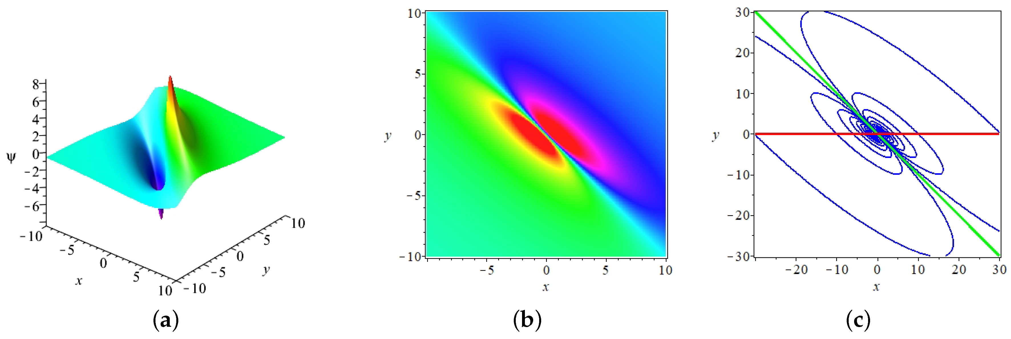
It can be noticed that the velocity of the one-lump wave (13) is available. On the $(x,y)$ plane, the velocity of lump wave along the x axis is $v_x^L=-\frac{(r_3{d}_1+r_8{f}_1^2)(c_1^2+d_1^2)+r_7(c_1{f}_1-e_1{d}_1)}{d_1}$, and the speed along the y axis is $v_y^L=\frac{2r_3{c}_1{d}_1+r_6{d}_1+r_7{f}_1+r_8(c_1{f}_1+e_1{d}_1)}{d_1}$.

Figure 2. (Color online) One-lump Solution (13) with $r_2=r_3=r_4=r_6=r_7=r_8=1,a_1=0,b_1=0,c_1=1,d_1=0.5,e_1=0.3,f_1=-0.8.$ (a) The three-dimensional stereograms when $t=0,z=0.$ (b) the corresponding contour figure. (c) Characteristic lines figure, the red line ($y=0$) and the green line ($x+y=0$) are two characteristic lines of the one-lump wave.

Figure 2. (Color online) One-lump Solution (13) with $r_2=r_3=r_4=r_6=r_7=r_8=1,a_1=0,b_1=0,c_1=1,d_1=0.5,e_1=0.3,f_1=-0.8.$ (a) The three-dimensional stereograms when $t=0,z=0.$ (b) the corresponding contour figure. (c) Characteristic lines figure, the red line ($y=0$) and the green line ($x+y=0$) are two characteristic lines of the one-lump wave.

Based on the analysis of the transformation mechanism of the breathers [33,34,35,36], some conclusions about the one-breather solution (9) of Equation (3) can be discussed.

(1)

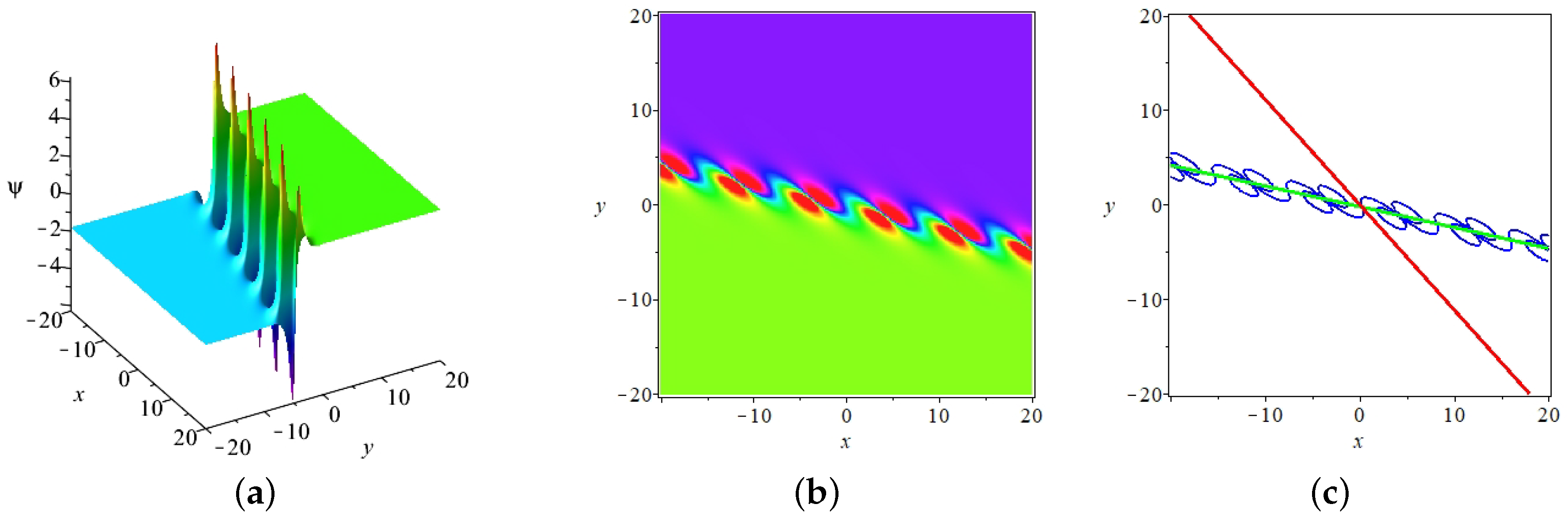
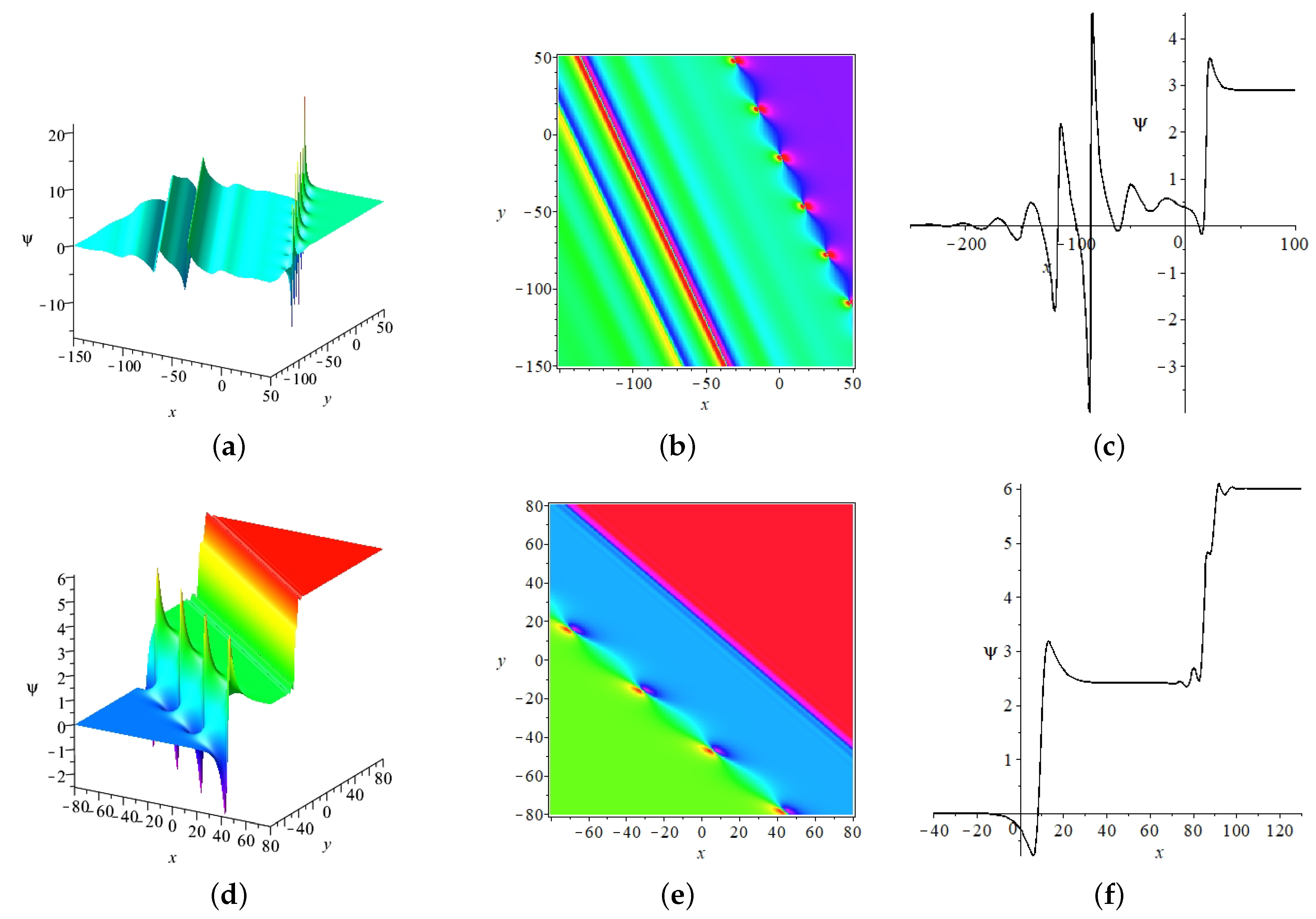
It is obvious from expression (9) that the one-breather solution contains a trigonometric function $(sin,cos)$ and a hyperbolic function $(cosh,sinh)$, in which the localized properties of the one-breather are controlled by the hyperbolic function, and the periodic properties are decided by the trigonometric function, so the one-breather can be considered to be the combination of the soliton wave and periodic wave.

(2)

Two characteristic lines of the one-breather have the form of ${\theta }_1+\frac{1}{2}ln{\beta }_2=a_{1}x+(a_1{c}_1-b_1{d}_1)y+(a_1{e}_1-b_1{f}_1)z+(a_1{w}_{1R}-b_1{w}_{1I})t+{\gamma }_1+\frac{1}{2}ln{\beta }_2$ and ${\Lambda }_1=b_{1}x+(a_1{d}_1+b_1{c}_1)y+(a_1{f}_1+b_1{e}_1)z+(a_1{w}_{1I}+b_1{w}_{1R})t+{\kappa }_1.$

(3)

It can be noticed that the velocities of the soliton along the x axis and y axis can be written as $v_x^s=-\frac{a_1(a_1{w}_{1R}-b_1{w}_{1I})}{{a_1}^2+{(a_1{c}_1-b_1{d}_1)}^2}$ and $v_y^s=-\frac{(a_1{c}_1-b_1{d}_1)(a_1{w}_{1R}-b_1{w}_{1I})}{{a_1}^2+{(a_1{c}_1-b_1{d}_1)}^2}$, respectively; the velocities of periodic wave along x axis and y axis are $v_x^p=-\frac{b_1(a_1{w}_{1I}+b_1{w}_{1R})}{{b_1}^2+{(a_1{d}_1+b_1{c}_1)}^2}$ and $v_y^p=-\frac{(a_1{d}_1+b_1{c}_1)(a_1{w}_{1I}+b_1{w}_{1R})}{{b_1}^2+{(a_1{d}_1+b_1{c}_1)}^2}$, respectively; the above results are discussed on the plane $(x,y)$, and similar conclusions can be obtained on the $(x,z)$ plane and $(y,z)$ plane.

(i)

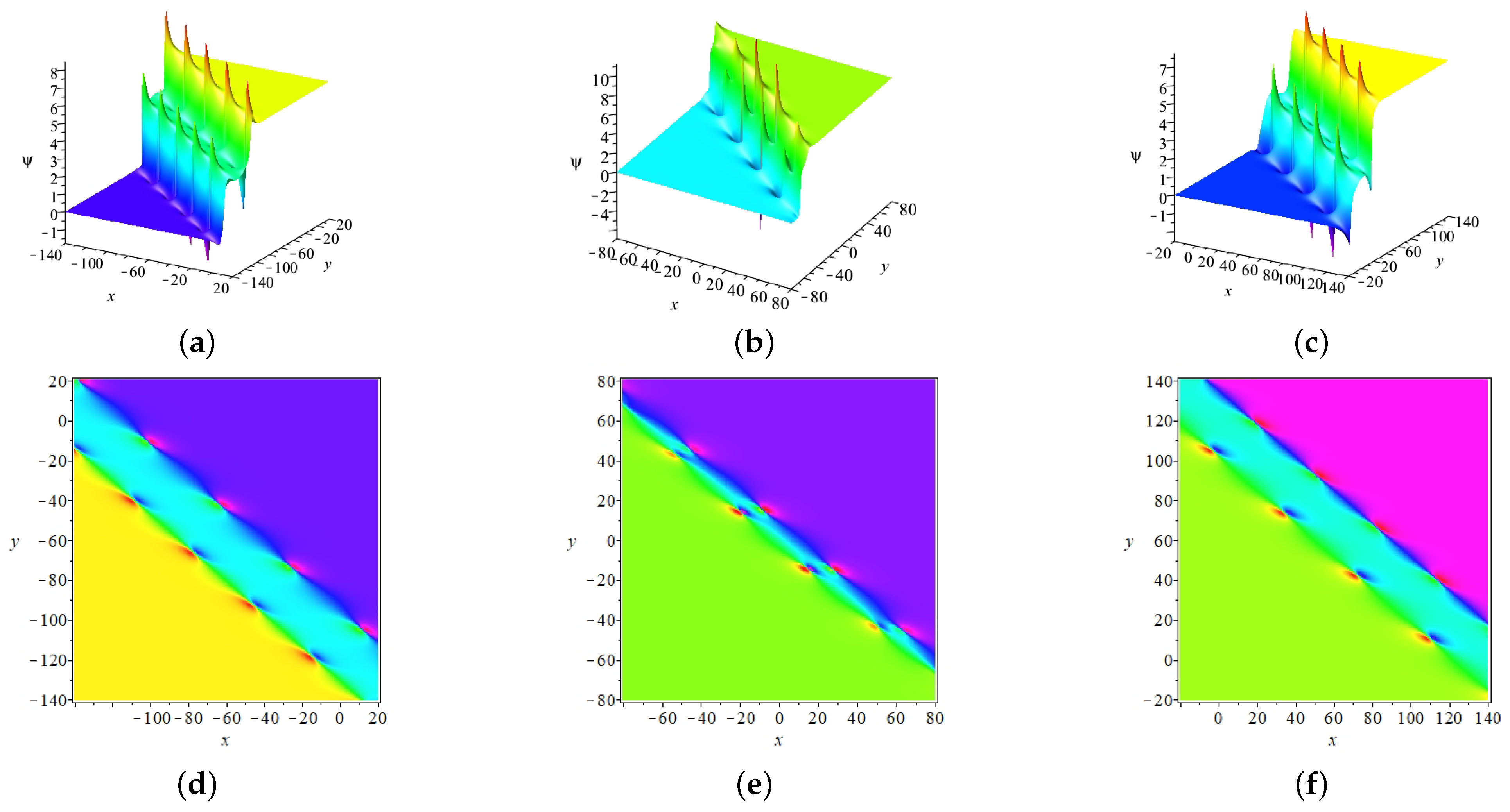
If the relationship $\left|\begin{array}{cc}{a}_1& a_1{c}_1-b_1{d}_1\\ b_1& a_1{d}_1+b_1{c}_1\end{array}\right|\ne 0$ is satisfied, i.e., $d_1\ne 0,$ the two characteristic lines ${\theta }_1+\frac{1}{2}ln{\beta }_2$ and ${\Lambda }_1$ will not be parallel in the plane $(x,y)$, as shown in Figure 1.

(ii)

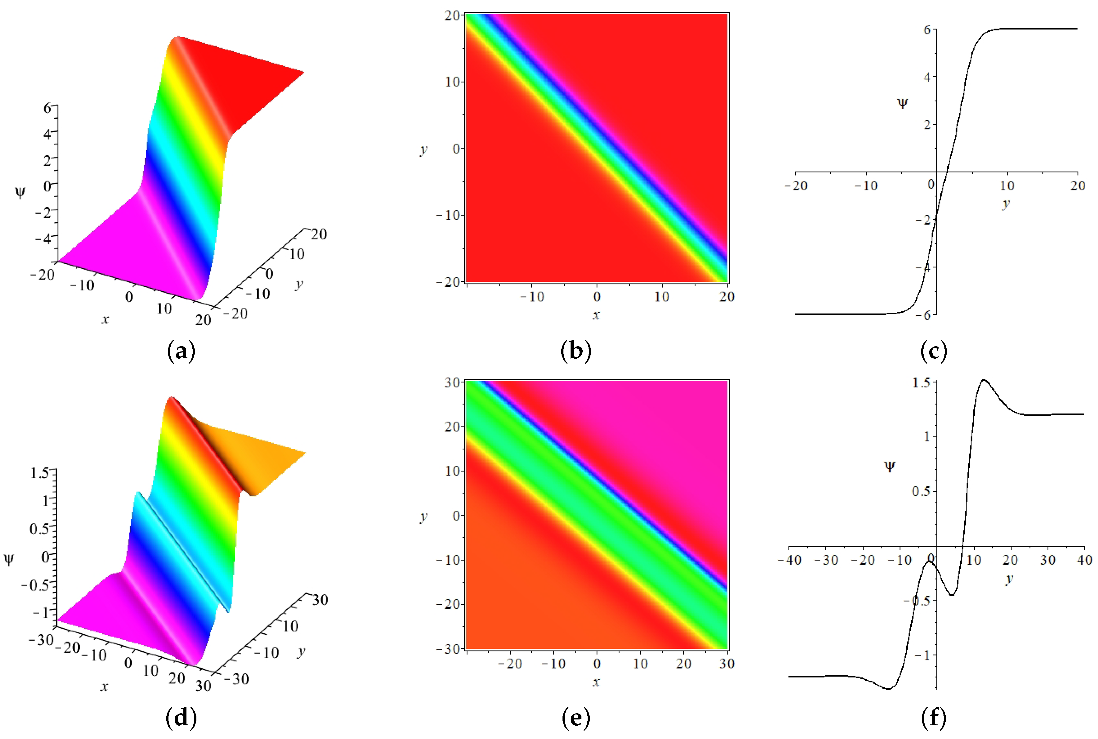
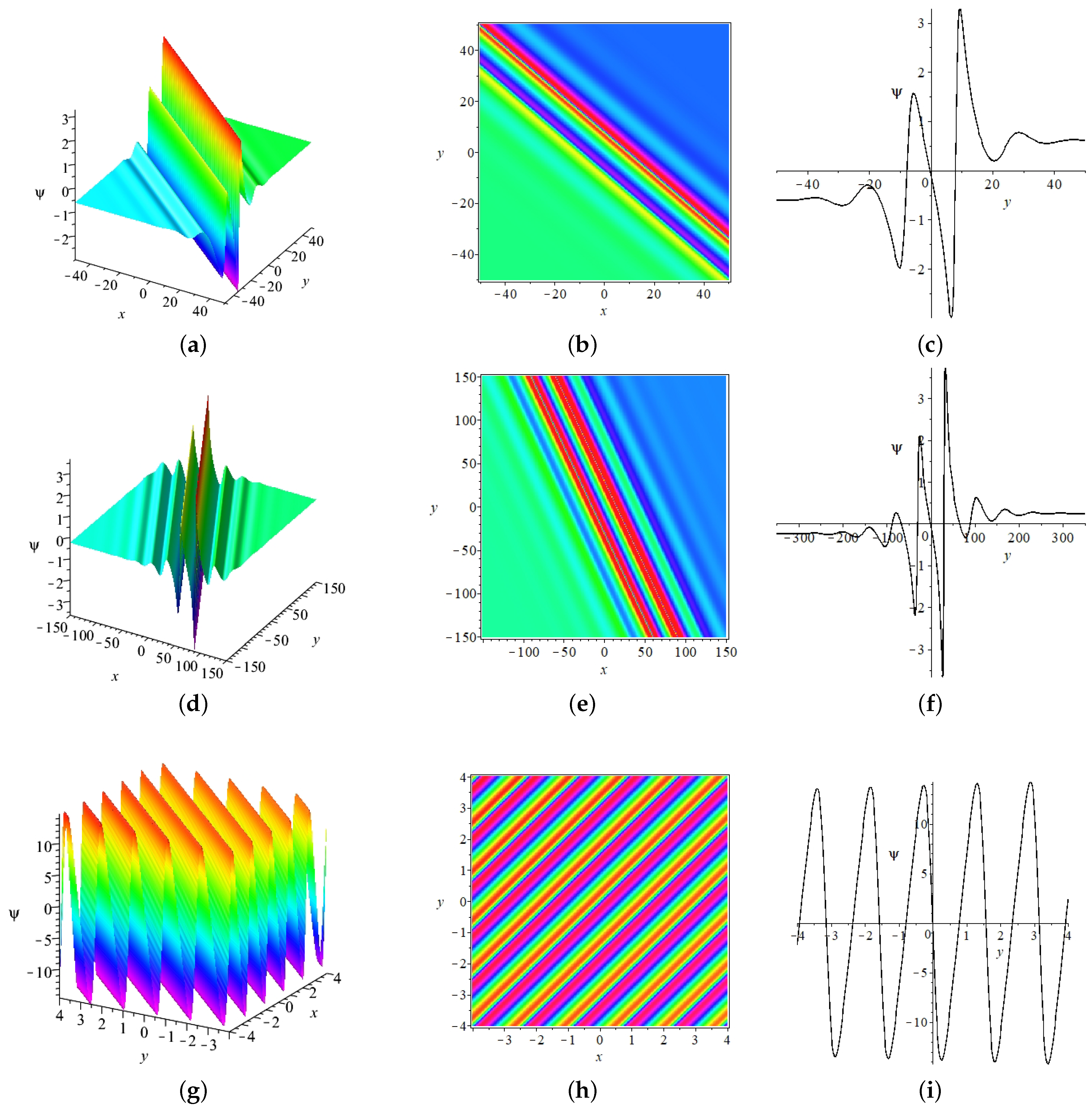
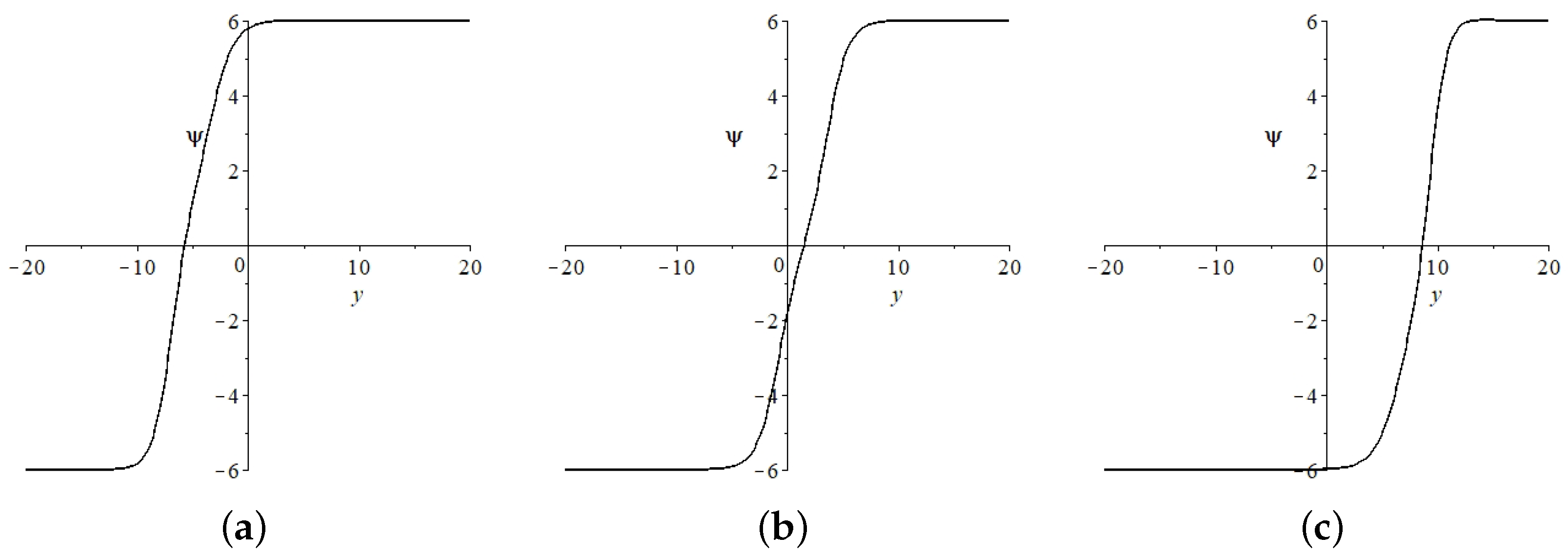
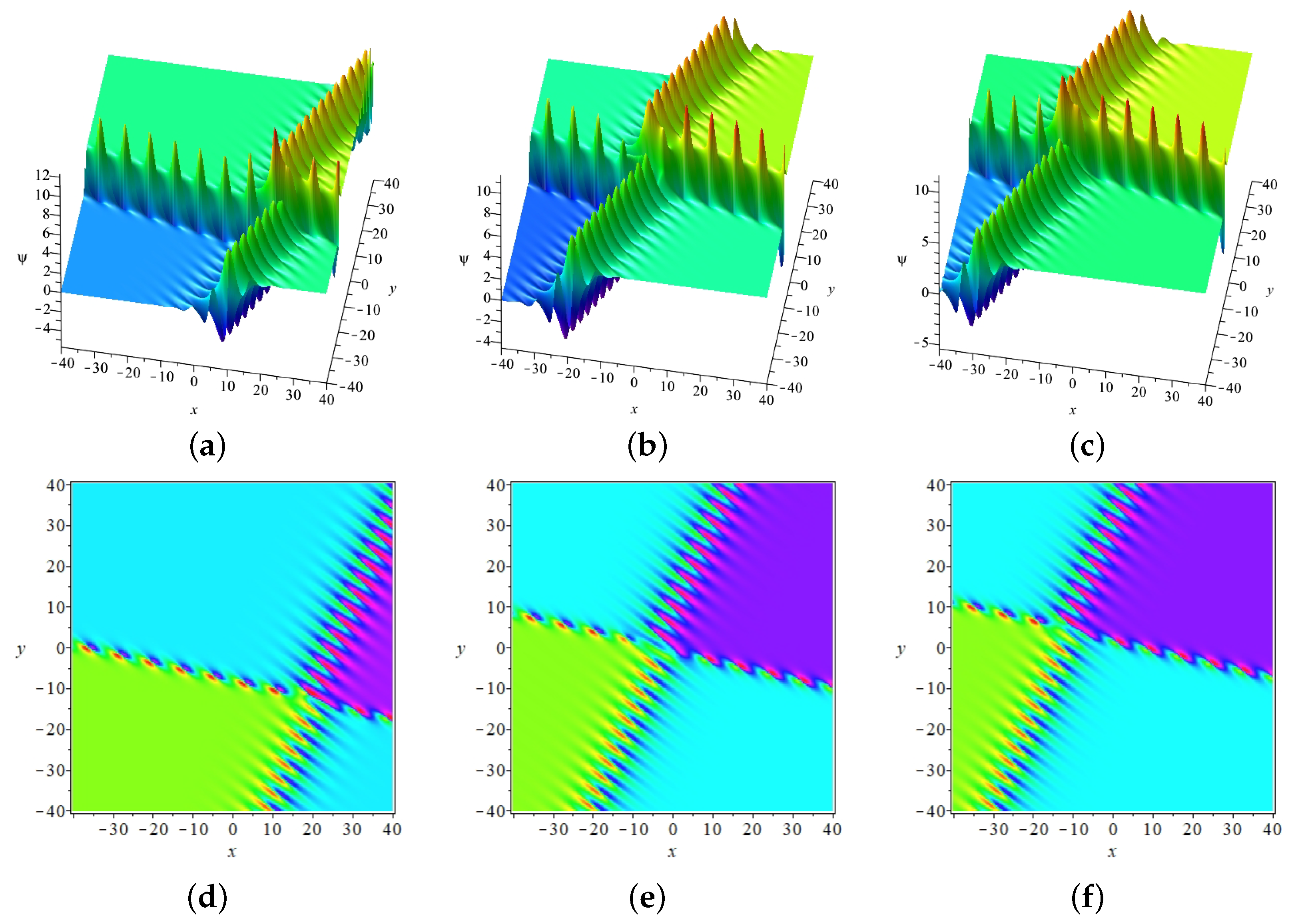
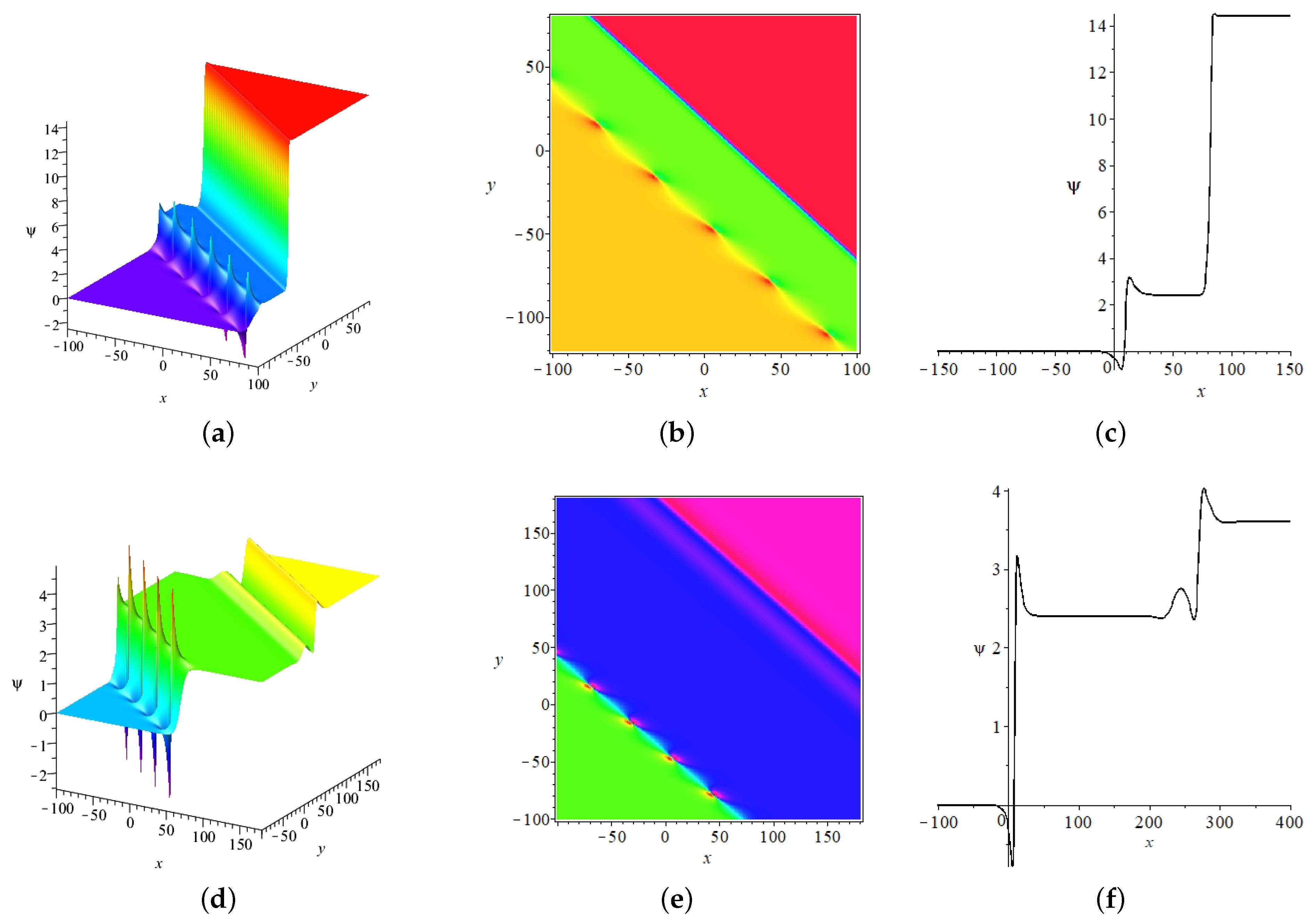
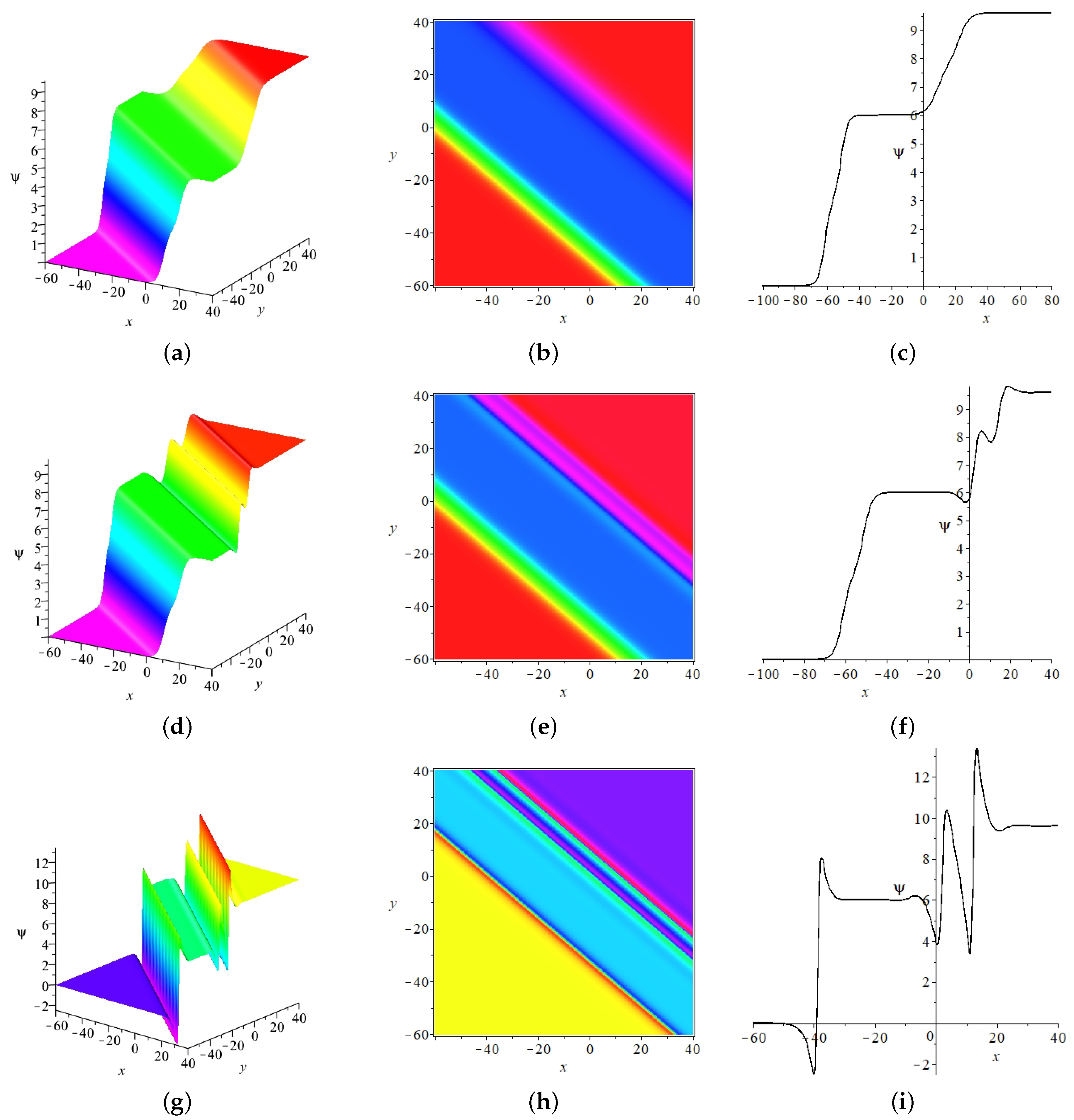
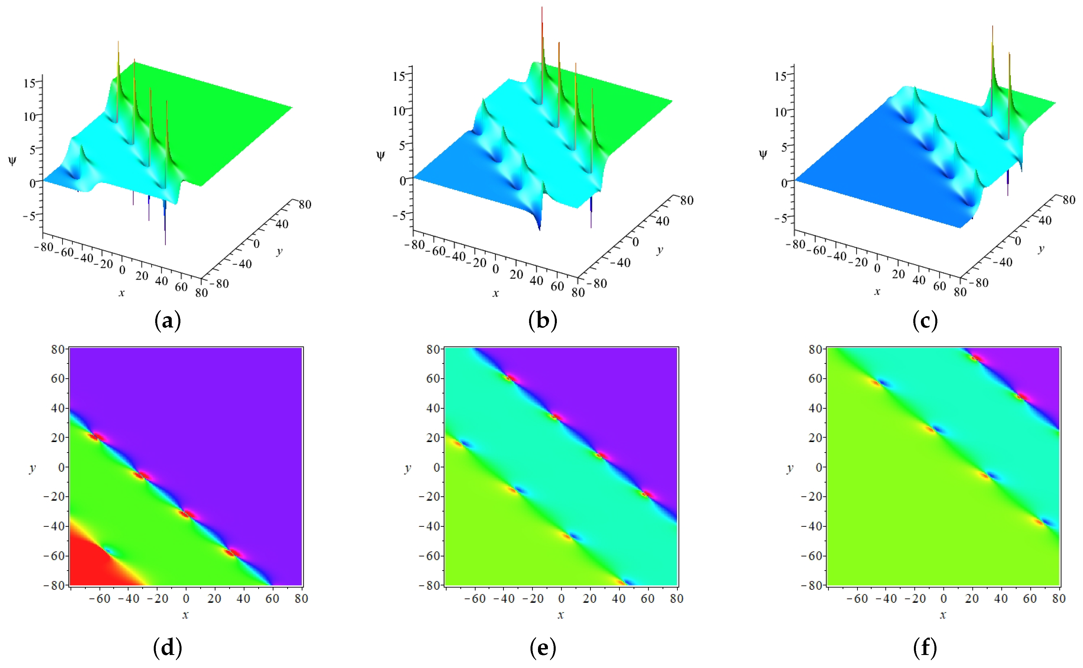
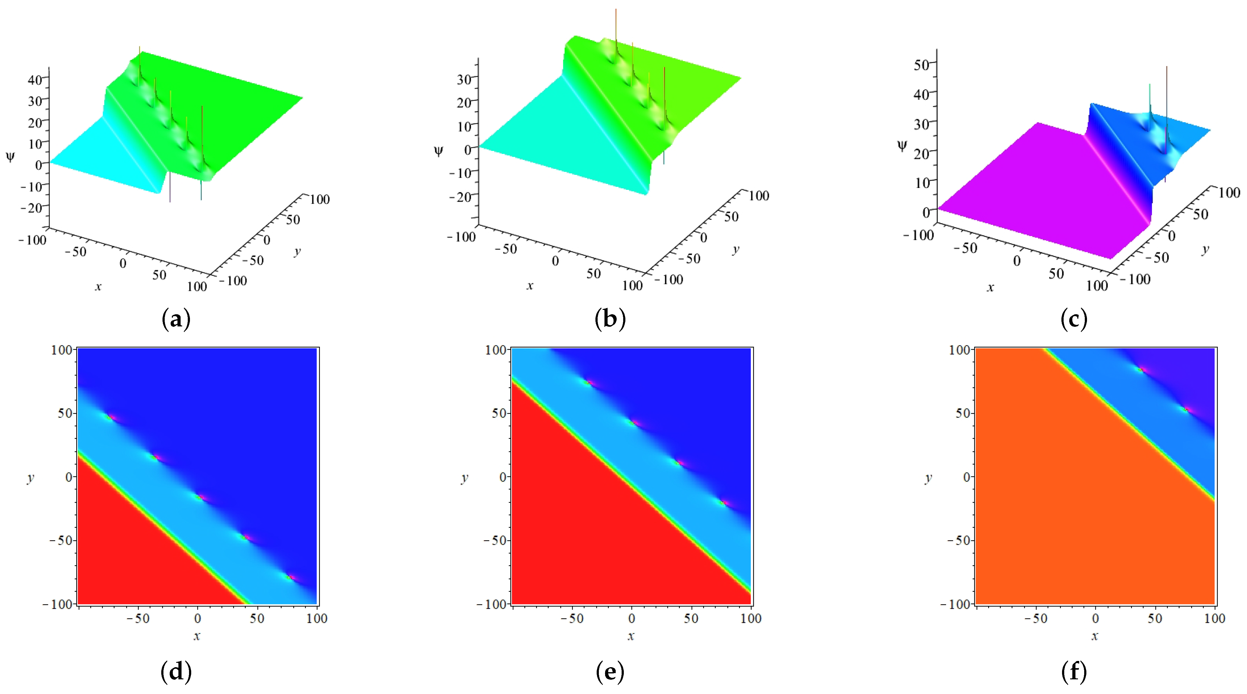
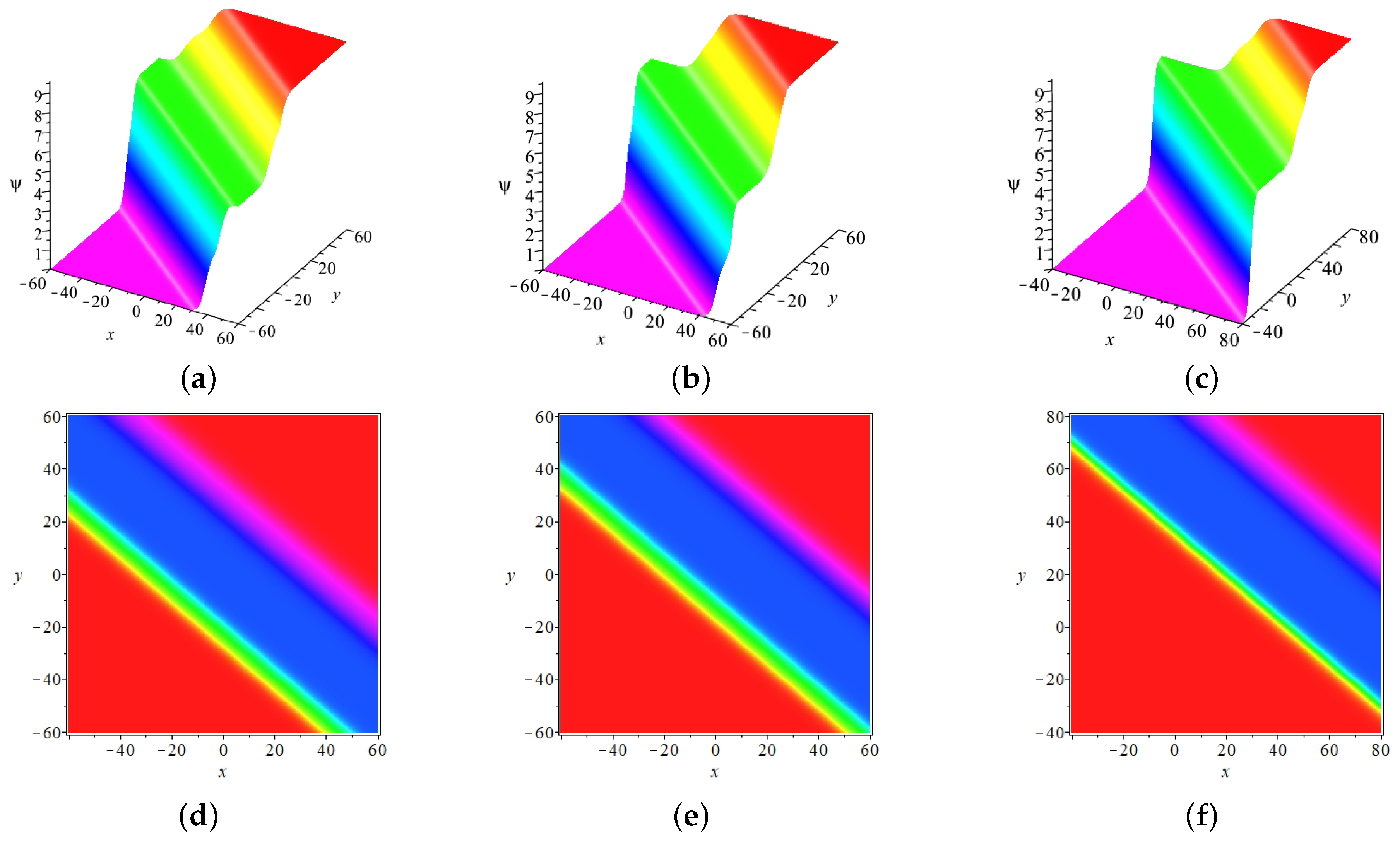
If the relationship $\left|\begin{array}{cc}{a}_1& a_1{c}_1-b_1{d}_1\\ b_1& a_1{d}_1+b_1{c}_1\end{array}\right|=0$ is satisfied, i.e., $d_1=0,$ the two characteristic lines ${\theta }_1+\frac{1}{2}ln{\beta }_2$ and ${\Lambda }_1$ will be parallel, as shown in Figure 3 and Figure 4. Under special conditions, the one-breather can be converted into a series of nonlinear waves which include quasi-kink soliton, M-shaped kink soliton, oscillation M-shaped kink soliton, multi-peak kink soliton and quasi-periodic wave. In Figure 3a–c, the one-breather will be a transformed quasi-kink soliton $(\frac{b_1}{a_1}=0.1)$, which has one characteristic line and presents the shape of a ladder. In Figure 3d–f, the M-shaped kink soliton $(\frac{b_1}{a_1}=1)$ has two peaks and one valley, and appears in the shape of M climbing upward. With the increase of value of $\frac{b_1}{a_1}$, the one-breather will become an oscillation M-shaped kink soliton $(\frac{b_1}{a_1}=3)$, and the number of characteristic lines also increases. If the value of $\frac{b_1}{a_1}$ keeps growing, the periodicity will become obvious, then the one-breather will become an asymmetric multi-peak kink soliton $(\frac{b_1}{a_1}=5)$, as shown in Figure 4a–f. When the value $\frac{b_1}{a_1}$ becomes very large, the one-breather will be transformed into a quasi-periodic wave $(\frac{b_1}{a_1}=1000)$, as shown in Figure 4g–i. Gradually, with the values of $\frac{b_1}{a_1}$ increasing, their periodicity becomes more and more obvious and their locality almost disappears.

Remark 2. 

Figure 5 shows that quasi-kink soliton moves along the y axis at a different time. Then, the other figure of the transformation mechanism of breathers at a different time can also be obtained similarly.

4. Two-Breather Solution, Transformation Mechanism and Molecular State

4.1. Two-Breather Solution of Equation (3)

In this section, we investigate the transformation mechanism of the two-breather wave. The four-soliton solution can be written as

$$\begin{array}{c}\hfill {\xi }_4=1+{\mathrm{e}}^{{\epsilon }_1}+{\mathrm{e}}^{{\epsilon }_2}+{\mathrm{e}}^{{\epsilon }_3}+{\mathrm{e}}^{{\epsilon }_4}+{\mathrm{e}}^{{\epsilon }_1+{\epsilon }_2+{\mathrm{A}}_{12}}+{\mathrm{e}}^{{\epsilon }_1+{\epsilon }_3+{\mathrm{A}}_{13}}+{\mathrm{e}}^{{\epsilon }_1+{\epsilon }_4+{\mathrm{A}}_{14}}+{\mathrm{e}}^{{\epsilon }_2+{\epsilon }_3+{\mathrm{A}}_{23}}\\ \hfill +{\mathrm{e}}^{{\epsilon }_2+{\epsilon }_4+{\mathrm{A}}_{24}}+{\mathrm{e}}^{{\epsilon }_3+{\epsilon }_4+{\mathrm{A}}_{34}}+{\mathrm{e}}^{{\epsilon }_1+{\epsilon }_2+{\epsilon }_3+{\mathrm{A}}_{12}+{\mathrm{A}}_{23}+{\mathrm{A}}_{13}}+{\mathrm{e}}^{{\epsilon }_1+{\epsilon }_2+{\epsilon }_4+{\mathrm{A}}_{12}+{\mathrm{A}}_{24}+{\mathrm{A}}_{14}}\\ \hfill +{\mathrm{e}}^{{\epsilon }_1+{\epsilon }_3+{\epsilon }_4+{\mathrm{A}}_{13}+{\mathrm{A}}_{34}+{\mathrm{A}}_{14}}+{\mathrm{e}}^{{\epsilon }_2+{\epsilon }_3+{\epsilon }_4+{\mathrm{A}}_{23}+{\mathrm{A}}_{34}+{\mathrm{A}}_{24}}+{\mathrm{e}}^{{\epsilon }_1+{\epsilon }_2+{\epsilon }_3+{\epsilon }_4+{\mathrm{A}}_{12}+{\mathrm{A}}_{23}+{\mathrm{A}}_{13}+{\mathrm{A}}_{23}+{\mathrm{A}}_{34}+{\mathrm{A}}_{24}}.\end{array}$$

(14)

Letting

$$u_3=a_2+b_2\mathrm{i},u_4=a_2-b_2\mathrm{i},v_3=c_2+d_2\mathrm{i},v_4=c_2-d_2\mathrm{i},h_3=e_2+f_2\mathrm{i},h_4=e_2-f_2\mathrm{i},$$

$${{\epsilon }_3}^{\left(0\right)}=ln\frac{{\beta }_3}{2}+{\gamma }_2+{\kappa }_2\mathrm{i},{{\epsilon }_4}^{\left(0\right)}=ln\frac{{\beta }_3}{2}+{\gamma }_2-{\kappa }_2\mathrm{i},$$

(15)

where $a_2,b_2,c_2,d_2,e_2,f_2\ne 0,{\beta }_3>0,{\gamma }_2$ and ${\kappa }_2$ are arbitrary real constants, then substituting (10) and (15) into (14), we obtain

$${\xi }_4=1+{\beta }_1{\mathrm{e}}^{{\theta }_1}cos\left({\Lambda }_1\right)+\frac{{{\beta }_1}^2{G}_1{\mathrm{e}}^{2{\theta }_1}}{4}+{\beta }_3{\mathrm{e}}^{{\theta }_2}cos\left({\Lambda }_2\right)+\frac{{{\beta }_3}^2{G}_2{\mathrm{e}}^{2{\theta }_2}}{4}$$

$$+\frac{{{\beta }_1}^2{{\beta }_3}^2{G}_1{G}_2}{16}{\mathrm{e}}^{2{\theta }_1+2{\theta }_2}(M_{3R}^2+M_{3I}^2)(M_{4R}^2+M_{4I}^2)$$

$$+\frac{{\beta }_1{\beta }_3}{2}{\mathrm{e}}^{{\theta }_1+{\theta }_2}(M_{3R}cos({\Lambda }_1+{\Lambda }_2)-M_{3I}sin({\Lambda }_1+{\Lambda }_2))$$

$$+\frac{{\beta }_1{\beta }_3}{2}{\mathrm{e}}^{{\theta }_1+{\theta }_2}(M_{4R}cos({\Lambda }_1-{\Lambda }_2)-M_{4I}sin({\Lambda }_1-{\Lambda }_2))$$

$$+\frac{{{\beta }_1}^2{\beta }_3{G}_1}{4}{\mathrm{e}}^{2{\theta }_1+{\theta }_2}((M_{3R}{M}_{4R}+M_{3I}{M}_{4I})cos\left({\Lambda }_2\right)-(M_{3I}{M}_{4R}-M_{3R}{M}_{4I})sin\left({\Lambda }_2\right))$$

$$+\frac{{\beta }_1{{\beta }_3}^2{G}_2}{4}{\mathrm{e}}^{{\theta }_1+2{\theta }_2}((M_{3R}{M}_{4R}-M_{3I}{M}_{4I})cos\left({\Lambda }_1\right)-(M_{3I}{M}_{4R}+M_{3R}{M}_{4I})sin\left({\Lambda }_1\right)),$$

(16)

where

$${\theta }_2=a_{2}x+(a_2{c}_2-b_2{d}_2)y+(a_2{e}_2-b_2{f}_2)z+(a_2{w}_{2R}-b_2{w}_{2I})t+{\gamma }_2,$$

$${\Lambda }_2=b_{2}x+(a_2{d}_2+b_2{c}_2)y+(a_2{f}_2+b_2{e}_2)z+(a_2{w}_{2I}+b_2{w}_{2R})t+{\kappa }_2,{\beta }_4=\frac{{{\beta }_3}^2{G}_2}{4},$$

$$G_2=\frac{-4r_2(a_2{b}_2{f}_2+3b_2^2{e}_2)+4r_3{d}_2^2-16r_8{d}_2^2{f}_2^2}{-4r_2(a_2{b}_2{f}_2-3a_2^2{e}_2)+4r_3{d}_2^2-16r_8{d}_2^2{f}_2^2},$$

$$w_{2R}=-r_2(a_2^2{e}_2-b_2^2{e}_2-2a_2{b}_2{f}_2)-r_3{c}_2^2-d_2^2-r_6{c}_2-r_7{e}_2-r_8(c_2{e}_2-d_2{f}_2),$$

$$w_{2I}=-r_2(a_2^2{f}_2-b_2^2{f}_2+2a_2{b}_2{e}_2)-2r_3{c}_2{d}_2-r_6{d}_2-r_7{f}_2-r_8(c_2{f}_2+e_2{d}_2).$$

$$M_{3R}=\mathrm{Re}\left({\mathrm{e}}^{{\mathrm{A}}_{13}}\right),M_{3I}=\mathrm{Im}\left({\mathrm{e}}^{{\mathrm{A}}_{13}}\right),M_{4R}=\mathrm{Re}\left({\mathrm{e}}^{{\mathrm{A}}_{14}}\right),M_{4I}=\mathrm{Im}\left({\mathrm{e}}^{{\mathrm{A}}_{14}}\right).$$

Unlike the one-breather, the two-breather has two sets of characteristic lines, i.e., ${\theta }_1+\frac{1}{2}ln{\beta }_2=a_{1}x+(a_1{c}_1-b_1{d}_1)y+(a_1{e}_1-b_1{f}_1)z+(a_1{w}_{1R}-b_1{w}_{1I})t+{\gamma }_1+\frac{1}{2}ln{\beta }_2,{\Lambda }_1=b_{1}x+(a_1{d}_1+b_1{c}_1)y+(a_1{f}_1+b_1{e}_1)z+(a_1{w}_{1I}+b_1{w}_{1R})t+{\kappa }_1,$ and ${\theta }_2+\frac{1}{2}ln{\beta }_4=a_{2}x+(a_2{c}_2-b_2{d}_2)y+(a_2{e}_2-b_2{f}_2)z+(a_2{w}_{2R}-b_2{w}_{2I})t+{\gamma }_2+\frac{1}{2}ln{\beta }_4,{\Lambda }_2=b_{2}x+(a_2{d}_2+b_2{c}_2)y+(a_2{f}_2+b_2{e}_2)z+(a_2{w}_{2I}+b_2{w}_{2R})t+{\kappa }_2.$

Proposition 1. 

If one satisfies

$$\left|\begin{array}{cc}{a}_1& a_1{c}_1-b_1{d}_1\\ b_1& a_1{d}_1+b_1{c}_1\end{array}\right|\ne 0,\left|\begin{array}{cc}{a}_2& a_2{c}_2-b_2{d}_2\\ b_2& a_2{d}_2+b_2{c}_2\end{array}\right|\ne 0,$$

the two sets of waves are two-breathers on the plane $(x,y)$.

(1)

If the two-breather satisfies $\left|\begin{array}{cc}{a}_1& a_1{c}_1-b_1{d}_1\\ a_2& a_2{c}_2-b_2{d}_2\end{array}\right|=0,$ i.e., the two-breather is parallel, whereas they will only collide at a certain time due to different speeds, which is called the short-lived collision, as shown in Figure 6.

(2)

If the two-breather satisfies $\left|\begin{array}{cc}{a}_1& a_1{c}_1-b_1{d}_1\\ a_2& a_2{c}_2-b_2{d}_2\end{array}\right|\ne 0,$ i.e., the two-breather is not parallel; in other words, they will always be in a state of intersection, which is called the long-lived collision, as shown in Figure 7.

Figure 6. (Color online) The collision between parallel two-breathers with $r_2=r_3=r_4=r_6=r_7=r_8=1,a_1=0.3,b_1=0,c_1=1.2,d_1=0.8,e_1=0.75,f_1=0.75,{\beta }_1=2,{\gamma }_1=0,{\kappa }_1=0,a_2=0.2,b_2=0,c_2=1.2,d_2=1,e_2=\frac{2}{3},f_2=\frac{2}{3},{\beta }_3=2,{\gamma }_2=0,{\kappa }_2=0.$ (a–c) are vertical view when $t=-50,t=0$ and $t=50.$ (d–f) are contour plots.

Figure 6. (Color online) The collision between parallel two-breathers with $r_2=r_3=r_4=r_6=r_7=r_8=1,a_1=0.3,b_1=0,c_1=1.2,d_1=0.8,e_1=0.75,f_1=0.75,{\beta }_1=2,{\gamma }_1=0,{\kappa }_1=0,a_2=0.2,b_2=0,c_2=1.2,d_2=1,e_2=\frac{2}{3},f_2=\frac{2}{3},{\beta }_3=2,{\gamma }_2=0,{\kappa }_2=0.$ (a–c) are vertical view when $t=-50,t=0$ and $t=50.$ (d–f) are contour plots.

Figure 7. (Color online) The collision between non-parallel two-breather with $r_2=r_3=r_4=r_6=r_7=r_8=1,a_1=0.3,b_1=1,c_1=1.2,d_1=-1,e_1=1,f_1=1,{\beta }_1=2,{\gamma }_1=0,{\kappa }_1=0,a_2=0.3,b_2=1,c_2=1.2,d_2=0.5,e_2=0.5,f_2=1,{\beta }_3=2,{\gamma }_2=0,{\kappa }_2=0.$ (a–c) are vertical view when $t=-3,t=0$ and $t=1.$ (d–f) are contour plots.

Figure 7. (Color online) The collision between non-parallel two-breather with $r_2=r_3=r_4=r_6=r_7=r_8=1,a_1=0.3,b_1=1,c_1=1.2,d_1=-1,e_1=1,f_1=1,{\beta }_1=2,{\gamma }_1=0,{\kappa }_1=0,a_2=0.3,b_2=1,c_2=1.2,d_2=0.5,e_2=0.5,f_2=1,{\beta }_3=2,{\gamma }_2=0,{\kappa }_2=0.$ (a–c) are vertical view when $t=-3,t=0$ and $t=1.$ (d–f) are contour plots.

4.2. Transformation Mechanism of Two-Breather for Equation (3)

In this section, the transformation mechanism of the two-breather is studied systematically. According to the one-breather transformation mechanism, we know that the breathers can be converted into a series of nonlinear localized waves. Then, the investigation of the two-breather transformation mechanism can be divided into three aspects, including the modes of non-, semi-, and full transformation.

Regarding non-transformed modes, it is obvious that the two-breather will not be converted, as shown in Figure 6 and Figure 7. Regarding semi-transformed modes, that is one where the two-breather is transformed.

Proposition 2. 

If one satisfies

$$\left|\begin{array}{cc}{a}_1& a_1{c}_1-b_1{d}_1\\ b_1& a_1{d}_1+b_1{c}_1\end{array}\right|=0,\left|\begin{array}{cc}{a}_2& a_2{c}_2-b_2{d}_2\\ b_2& a_2{d}_2+b_2{c}_2\end{array}\right|\ne 0,$$

i.e., $d_1=0$. Then, one of the two sets of waves is the breather, the other can be converted into a series of nonlinear waves including the quasi-kink soliton, M-shaped kink soliton, oscillation M-shaped kink soliton, and multi-peak kink soliton, as shown in Figure 8 and Figure 9. In Figure 8a–c, one of the two-breathers is transformed into the quasi-kink soliton. In Figure 8d–e, it is transformed into the M-shaped kink soliton. In Figure 9a–c, one of the two-breathers is transformed into the oscillation M-shaped kink soliton. In Figure 9d–e, it is transformed into the multi-peak kink soliton.

For the full-transformation modes, the two-breather will be transformed into a series of nonlinear waves.

Proposition 3. 

If one satisfies

$$\left|\begin{array}{cc}{a}_1& a_1{c}_1-b_1{d}_1\\ b_1& a_1{d}_1+b_1{c}_1\end{array}\right|=0,\left|\begin{array}{cc}{a}_2& a_2{c}_2-b_2{d}_2\\ b_2& a_2{d}_2+b_2{c}_2\end{array}\right|=0,$$

i.e., $d_1=d_2=0$, then, the two-breather will be transformed into a series of nonlinear waves including the quasi-kink soliton, M-shaped kink soliton, oscillation M-shaped kink soliton, and multi-peak kink soliton, as shown in Figure 10. In Figure 10a–c, the breathers are all transformed into quasi-kink solitons. In Figure 10d,e, they are transformed into the quasi-kink soliton and M-shaped kink soliton. In Figure 10g–i, they are transformed into the M-shaped kink soliton and oscillation M-shaped kink soliton.

It is worth noting that the above propositions are based on $\left|\begin{array}{cc}{a}_1& a_1{c}_1-b_1{d}_1\\ a_2& a_2{c}_2-b_2{d}_2\end{array}\right|=0,$ which means the characteristic lines ${\theta }_1$ and ${\theta }_2$ are parallel. The above two waves collide at a certain time due to their velocities being different, which is the so-called short-lived collision. If the characteristic lines ${\theta }_1$ and ${\theta }_2$ are not parallel, i.e., $\left|\begin{array}{cc}{a}_1& a_1{c}_1-b_1{d}_1\\ a_2& a_2{c}_2-b_2{d}_2\end{array}\right|\ne 0,$ which is called the long-lived collision due to two waves being in collision with time.

4.3. Molecular State of Transformed Two-Breather

Given the above discussion and analysis, we know that breathers can be transformed into a series of nonlinear localized waves that include the quasi-kink soliton, M-shaped kink soliton, oscillation M-shaped kink soliton, multi-peak kink soliton and quasi-periodic wave. Then, the different types of the molecular state of the transformed two-breather are investigated under the condition of the same speed, which can be called velocity resonance.

Then, we further consider the velocity resonance of the transformed two-breather. The propagation velocity of along the direction perpendicular to transformed two-breather is equal, i.e.,

$$\sqrt{v{{}_{1x}^s}^2+v{{}_{1y}^s}^2}=\sqrt{v{{}_{2x}^s}^2+v{{}_{2y}^s}^2},$$

then, the relative position of the transformed two-breather will not be changed by time t, where

$$v_{1x}^s=-\frac{a_1(a_1{w}_{1R}-b_1{w}_{1I})}{{a_1}^2+{(a_1{c}_1-b_1{d}_1)}^2},v_{2x}^s=-\frac{a_2(a_2{w}_{2R}-b_2{w}_{2I})}{{a_2}^2+{(a_2{c}_2-b_2{d}_2)}^2},$$

$$v_{1y}^s=-\frac{(a_1{c}_1-b_1{d}_1)(a_1{w}_{1R}-b_1{w}_{1I})}{{a_1}^2+{(a_1{c}_1-b_1{d}_1)}^2},v_{2y}^s=-\frac{(a_2{c}_2-b_2{d}_2)(a_2{w}_{2R}-b_2{w}_{2I})}{{a_2}^2+{(a_2{c}_2-b_2{d}_2)}^2}.$$

One important factor is that the molecular state is built on the condition of $\left|\begin{array}{cc}{a}_1& a_1{c}_1-b_1{d}_1\\ a_2& a_2{c}_2-b_2{d}_2\end{array}\right|$$=0,$ i.e., the transformed two-breather is parallel. Furthermore, the distance of the transformed two-breather is not zero; otherwise, it will always be in coincidence. The distance has the form of

$$\frac{\left|\left.({\gamma }_1+\frac{1}{2}ln{\beta }_2)-({\gamma }_2+\frac{1}{2}ln{\beta }_4)\right|\right.}{\sqrt{a_1^2+{(a_1{c}_1-b_1{d}_1)}^2}}.$$

Proposition 4. 

If the following conditions

$$\left|\begin{array}{cc}{a}_1& a_1{c}_1-b_1{d}_1\\ a_2& a_2{c}_2-b_2{d}_2\end{array}\right|=0,\left|\begin{array}{cc}{a}_1& a_1{c}_1-b_1{d}_1\\ b_1& a_1{d}_1+b_1{c}_1\end{array}\right|\ne 0,\left|\begin{array}{cc}{a}_2& a_2{c}_2-b_2{d}_2\\ b_2& a_2{d}_2+b_2{c}_2\end{array}\right|\ne 0,$$

and

$$v_{B_1}^s=v_{B_2}^s,\left|\left.({\gamma }_1+\frac{1}{2}ln{\beta }_2)-({\gamma }_2+\frac{1}{2}ln{\beta }_4)\right|\right.\ne 0,$$

are satisfied, the two-breather will not be transformed, which is called the mode of non-transformation, and the distance of the two-breather will not be changed by time, as shown in Figure 11.

Proposition 5. 

If the following conditions

$$\left|\begin{array}{cc}{a}_1& a_1{c}_1-b_1{d}_1\\ a_2& a_2{c}_2-b_2{d}_2\end{array}\right|=0,\left|\begin{array}{cc}{a}_1& a_1{c}_1-b_1{d}_1\\ b_1& a_1{d}_1+b_1{c}_1\end{array}\right|\ne 0,\left|\begin{array}{cc}{a}_2& a_2{c}_2-b_2{d}_2\\ b_2& a_2{d}_2+b_2{c}_2\end{array}\right|=0,$$

and

$$v_{B_1}^s=v_{B_2}^s,\left|\left.({\gamma }_1+\frac{1}{2}ln{\beta }_2)-({\gamma }_2+\frac{1}{2}ln{\beta }_4)\right|\right.\ne 0,$$

are satisfied, one of the two-breathers will be transformed, the other will not be, which is called the mode of semi-transformation, and the distance of one-breather and a nonlinear localized wave will not be changed by time, as shown in Figure 12.

Proposition 6. 

If the following conditions

$$\left|\begin{array}{cc}{a}_1& a_1{c}_1-b_1{d}_1\\ a_2& a_2{c}_2-b_2{d}_2\end{array}\right|=0,\left|\begin{array}{cc}{a}_1& a_1{c}_1-b_1{d}_1\\ b_1& a_1{d}_1+b_1{c}_1\end{array}\right|=0,\left|\begin{array}{cc}{a}_2& a_2{c}_2-b_2{d}_2\\ b_2& a_2{d}_2+b_2{c}_2\end{array}\right|=0,$$

and

$$v_{B_1}^s=v_{B_2}^s,\left|\left.({\gamma }_1+\frac{1}{2}ln{\beta }_2)-({\gamma }_2+\frac{1}{2}ln{\beta }_4)\right|\right.\ne 0,$$

are satisfied, the two-breather will be both transformed, which is called the mode of full transformation, and the distance of two nonlinear localized waves will not be changed by time, as shown in Figure 13.

5. Conclusions

In this paper, we focus on investigating breather solutions, transformation mechanisms, and the molecular state of the transformed two-breather. The N-soliton solutions are obtained using Hirota’s bilinear method. Then, it can be concluded that Equation (3) is integrable in the sense of N-soliton solutions. Furthermore, by using the complex conjugate conditions to the two- and four-soliton solution and imposing restrictions on the parameters, the one-breather solution, two-breather solution, and their transformation mechanism are analyzed systematically. The one-breather has two characteristic lines, ${\theta }_1+\frac{1}{2}ln{\beta }_2=a_{1}x+(a_1{c}_1-b_1{d}_1)y+(a_1{e}_1-b_1{f}_1)z+(a_1{w}_{1R}-b_1{w}_{1I})t+{\gamma }_1+\frac{1}{2}ln{\beta }_2$ and ${\Lambda }_1=b_{1}x+(a_1{d}_1+b_1{c}_1)y+(a_1{f}_1+b_1{e}_1)z+(a_1{w}_{1I}+b_1{w}_{1R})t+{\kappa }_1.$ If the condition $\left|\begin{array}{cc}{a}_1& a_1{c}_1-b_1{d}_1\\ b_1& a_1{d}_1+b_1{c}_1\end{array}\right|$ is not equal to zero, the one-breather will not be transformed, as shown in Figure 1. If the condition $\left|\begin{array}{cc}{a}_1& a_1{c}_1-b_1{d}_1\\ b_1& a_1{d}_1+b_1{c}_1\end{array}\right|$ is equal to zero, two characteristic lines are parallel, then the one-breather will be transformed. With the aid of the transformation mechanism of the nonlinear waves, the one-breather can be transformed into a series of nonlinear localized waves, such as the quasi-kink soliton, M-shaped kink soliton, oscillation M-shaped kink soliton, multi-peak kink soliton and quasi-periodic wave, as shown in Figure 3 and Figure 4. Then, the one-lump wave is obtained by taking the long-wave limit to the two-breather solution, as shown in Figure 2. The transformation mechanism of the two-breather is further studied similarly, as shown in Figure 8, Figure 9 and Figure 10. Furthermore, under the conditions of velocity resonance ($\sqrt{v{{}_{1x}^s}^2+v{{}_{1y}^s}^2}=\sqrt{v{{}_{2x}^s}^2+v{{}_{2y}^s}^2}$), the molecular state of the transformed two-breather is investigated systematically, which is shown in Figure 11, Figure 12 and Figure 13.

The phenomena presented in this paper are helpful to our further analysis of the complex dynamic behaviors in shallow-water waves, and play an important role in explaining the nonlinear phenomena existing in complex waves modeled by Equation (3). Furthermore, the dynamic behaviors of other high-dimensional integrable systems can be analyzed using the characteristic line method presented in this paper. It is worth noting that the characteristic line method cannot determine amplitude, which needs to be further studied.

References

- Mani Rajan, M.S.; Mahalingam, A. Nonautonomous solitons in modified inhomogeneous Hirota equation: Soliton control and soliton interaction. Nonlinear Dyn. 2015, 79, 2469–2484. [Google Scholar] [CrossRef]
- Ma, W.X. N-soliton solution of a combined pKP-BKP equation. J. Geom. Phys. 2021, 165, 104191. [Google Scholar] [CrossRef]
- Shen, Y.; Tian, B. Bilinear auto-Bäcklund transformations and soliton solutions of a (3+1)-dimensional generalized nonlinear evolution equation for the shallow water waves. Appl. Math. Lett. 2021, 122, 107301. [Google Scholar] [CrossRef]
- Mo, Y.F.; Ling, L.M.; Zeng, D.L. Data-driven vector soliton solutions of coupled nonlinear Schrödinger equation using a deep learning algorithm. Phys. Lett. A 2022, 421, 127739. [Google Scholar] [CrossRef]
- Wang, L.H.; Porsezian, K.; He, J.S. Breather and rogue wave solutions of a generalized nonlinear Schrödinger equation. Phys. Rev. E 2013, 87, 53202. [Google Scholar] [CrossRef] [Green Version]
- Feng, B.F.; Ma, R.Y.; Zhang, Y.J. General breather and rogue wave solutions to the complex short pulse equation. Phys. D 2022, 439, 133360. [Google Scholar] [CrossRef]
- Yusuf, A.; Sulaiman, T.A.; Alshomrani, A.S.; Baleanu, D. Breather and lump-periodic wave solutions to a system of nonlinear wave model arising in fluid mechanics. Nonlinear Dyn 2022, 110, 3655–3669. [Google Scholar] [CrossRef]
- Zhao, Z.L.; Chen, Y.; Han, B. Lump soliton, mixed lump stripe and periodic lump solutions of a (2+1)-dimensional asymmetrical Nizhnik-Novikov-Veselov equation. Modern Phys. Lett. B 2017, 31, 1750157. [Google Scholar] [CrossRef]
- Ma, W.X.; Zhou, Y. Lump solutions to nonlinear partial differential equations via Hirota bilinear forms. J. Differ. Equ. 2018, 264, 2633–2659. [Google Scholar] [CrossRef] [Green Version]
- Zhao, Z.L.; Yue, J.; He, L.C. New type of multiple lump and rogue wave solutions of the (2+1)-dimensional Bogoyavlenskii-Kadomtsev-Petviashvili equation. Appl. Math. Lett. 2022, 133, 108294. [Google Scholar] [CrossRef]
- Zhao, Z.L.; He, L.C.; Wazwaz, A.M. Dynamics of lump chains for the BKP equation describing propagation of nonlinear waves. Chin. Phys. B 2023, 32, 040501. [Google Scholar] [CrossRef]
- Zhao, Z.L.; He, L.C. Multiple lump molecules and interaction solutions of the Kadomtsev-Petviashvili I equation. Commun. Theor. Phys. 2022, 74, 105004. [Google Scholar] [CrossRef]
- Fan, E.G.; Hon, Y.C. Quasiperiodic waves and asymptotic behavior for Bogoyavlenskii’s breaking soliton equation in (2+1) dimensions. Phys. Rev. E 2008, 78, 36607. [Google Scholar] [CrossRef]
- Luo, L.; Fan, E.G. Bilinear approach to the quasi-periodic wave solutions of Modified Nizhnik-Novikov-Vesselov equation in (2+1) dimensions. Phys. Lett. A 2010, 374, 3001–3006. [Google Scholar] [CrossRef]
- Yue, J.; Zhao, Z.L. Solitons, breath-wave transitions, quasi-periodic waves and asymptotic behaviors for a (2+1)-dimensional Boussinesq-type equation. Eur. Phys. J. Plus 2022, 137, 914. [Google Scholar] [CrossRef]
- Li, J.; Sun, G.Q.; Jin, Z. Interactions of time delay and spatial diffusion induce the periodic oscillation of the vegetation system. Discrete Contin. Dyn. Syst. B 2022, 27, 2147–2172. [Google Scholar] [CrossRef]
- Zhou, T.Y.; Tian, B.; Chen, Y.Q.; Shen, Y. Painlevé analysis, auto-Bäcklund transformation and analytic solutions of a (2+1)-dimensional generalized Burgers system with the variable coefficients in a fluid. Nonlinear Dyn. 2022, 108, 2417–2428. [Google Scholar] [CrossRef]
- Dong, S.; Lan, Z.Z.; Gao, B.; Shen, Y.J. Bäcklund transformation and multi-soliton solutions for the discrete Korteweg-de Vries equation. Appl. Math. Lett. 2022, 125, 107747. [Google Scholar] [CrossRef]
- Yin, Y.H.; Lü, X.; Ma, W.X. Bäcklund transformation, exact solutions and diverse interaction phenomena to a (3+1)-dimensional nonlinear evolution equation. Nonlinear Dyn. 2022, 108, 4181–4194. [Google Scholar] [CrossRef]
- Mikhailov, A.V. The reduction problem and the inverse scattering method. Phys. D 1981, 3, 73–117. [Google Scholar] [CrossRef]
- Ning, T.K.; Chen, D.Y.; Zhang, D.J. The exact solutions for the nonisospectral AKNS hierarchy through the inverse scattering transform. Phys. A 2004, 339, 248–266. [Google Scholar] [CrossRef]
- Chen, M.S.; Fan, E.G.; He, J.S. l2-Sobolev space bijectivity of the scattering-inverse scattering transforms related to defocusing Ablowitz-Ladik systems. Phys. D 2023, 443, 133565. [Google Scholar] [CrossRef]
- Guo, B.L.; Ling, L.M.; Liu, Q.P. Nonlinear Schrödinger equation: Generalized Darboux transformation and rogue wave solutions. Phys. Rev. E 2012, 85, 26607. [Google Scholar] [CrossRef] [PubMed] [Green Version]
- Song, J.Y.; Xiao, Y.; Zhang, C.P. Darboux transformation, exact solutions and conservation laws for the reverse space-time Fokas-Lenells equation. Nonlinear Dyn. 2022, 107, 3805–3818. [Google Scholar] [CrossRef]
- Krichever, I.M. Methods of algebraic geometry in the theory of nonlinear equations. Russ. Math. Surv. 1977, 32, 185–213. [Google Scholar] [CrossRef]
- Cao, C.W.; Xiao, Y. Algebraic-geometric solution to (2+1)-dimensional Sawada-Kotera equation. Commun. Theor. Phys. 2008, 49, 34–36. [Google Scholar]
- Hirota, R. Exact solution of the Korteweg-de Vries equation for multiple collisions of solitons. Phys. Rev. Lett. 1971, 27, 1192–1194. [Google Scholar] [CrossRef]
- Hirota, R. The Direct Method in Soliton Theory; Cambridge University Press: Cambridge, UK, 2004. [Google Scholar]
- Bluman, G.W.; Yang, Z.Z. A symmetry-based method for constructing nonlocally related partial differential equation systems. J. Math. Phys. 2013, 54, 93504. [Google Scholar] [CrossRef] [Green Version]
- Liu, H.Z.; Li, J.B.; Zhang, Q.X. Lie symmetry analysis and exact explicit solutions for general Burgers’ equation. J. Comput. Appl. Math. 2009, 228, 1–9. [Google Scholar] [CrossRef] [Green Version]
- Zhao, Z.L.; Han, B. Lie symmetry analysis, Bäcklund transformations, and exact solutions of a (2+1)-dimensional Boiti-Leon-Pempinelli system. J. Math. Phys. 2017, 58, 101514. [Google Scholar] [CrossRef]
- Zhao, Z.L.; He, L.C. Lie symmetry, nonlocal symmetry analysis, and interaction of solutions of a (2+1)-dimensional KdV-mKdV equation. Theor. Math. Phys. 2021, 206, 142–162. [Google Scholar] [CrossRef]
- Zhang, X.; Wang, L.; Liu, C.; Li, M.; Zhao, Y.C. High-dimensional nonlinear wave transitions and their mechanisms. Chaos 2020, 30, 113107. [Google Scholar] [CrossRef]
- Zhang, X.; Wang, L.; Chen, W.Q.; Yao, X.M.; Wang, X.; Zhao, Y.C. Dynamics of transformed nonlinear waves in the (3+1)-dimensional B-type Kadomtsev-Petviashvili equation I: Transitions mechanisms. Commun. Nonlinear Sci. Numer. Simul. 2022, 105, 106070. [Google Scholar] [CrossRef]
- Yin, Z.Y.; Tian, S.F. Nonlinear wave transitions and their mechanisms of (2+1)-dimensional Sawada-Kotera equation. Phys. D 2021, 427, 133002. [Google Scholar] [CrossRef]
- Zhang, D.D.; Wang, L.; Liu, L.; Liu, T.X.; Sun, W.R. Shape-changed propagations and interactions for the (3+1)-dimensional generalized Kadomtsev-Petviashvili equation in fluids. Commun. Theor. Phys. 2021, 73, 95001. [Google Scholar] [CrossRef]
- Yao, X.M.; Wang, L.; Zhang, X.; Zhang, Y.B. Dynamics of transformed nonlinear waves in the (3+1)-dimensional B-type Kadomtsev-Petviashvili equation II: Interactions and molecular waves. Nonlinear Dyn. 2023, 111, 4613–4629. [Google Scholar] [CrossRef]
- Jia, M.; Lin, J.; Lou, S.Y. Soliton and breather molecules in few-cycle-pulse optical model. Nonlinear Dyn. 2020, 100, 3745–3757. [Google Scholar] [CrossRef]
- Yan, Z.W.; Lou, S.Y. Special types of solitons and breather molecules for a (2+1)-dimensional fifth-order KdV equation. Commun. Nonlinear Sci. Numer. Simul. 2020, 91, 105425. [Google Scholar] [CrossRef]
- Wang, M.M.; Qi, Z.Q.; Chen, J.C.; Li, B. Resonance Y-shaped soliton and interaction solutions in the (2+1)-dimensional B-type Kadomtsev-Petviashvili equation. Internat. J. Modern Phys. B 2021, 35, 2150222. [Google Scholar] [CrossRef]
- Zhang, Z.; Yang, S.X.; Li, B. Soliton molecules, asymmetric solitons and hybrid solutions for (2+1)-dimensional fifth-order KdV equation. Chinese Phys. Lett. 2019, 36, 120501. [Google Scholar] [CrossRef]
- Zhao, Z.L.; He, L.C. Nonlinear superposition between lump waves and other waves of the (2+1)-dimensional asymmetrical Nizhnik-Novikov-Veselov equation. Nonlinear Dyn. 2022, 108, 555–568. [Google Scholar] [CrossRef]
- Yue, J.; Zhao, Z.L. Interaction solutions and molecule state between resonance Y-type solitons and lump waves, and transformed 2-breather molecular waves of a (2+1)-dimensional asymmetrical Nizhnik-Novikov-Veselov equation. Nonlinear Dyn. 2023, 111, 7565–7589. [Google Scholar] [CrossRef]
- Yu, S.J.; Toda, K.; Sasa, N.; Fukuyama, T. N soliton solutions to the Bogoyavlenskii-Schiff equation and a quest for the soliton solution in (3+1) dimensions. J. Phys. A: Math. Gen. 1998, 31, 3337–3347. [Google Scholar] [CrossRef]
- Yin, H.M.; Tian, B.; Chai, J.; Wu, X.Y.; Sun, W.R. Solitons and bilinear Bäcklund transformations for a (3+1)-dimensional Yu-Toda-Sasa-Fukuyama equation in a liquid or lattice. Appl. Math. Lett. 2016, 58, 178–183. [Google Scholar] [CrossRef]
- Guo, H.D.; Xia, T.C.; Hu, B.B. Dynamics of abundant solutions to the (3+1)-dimensional generalized Yu-Toda-Sasa-Fukuyama equation. Appl. Math. Lett. 2020, 105, 106301. [Google Scholar] [CrossRef]
- Shen, Y.; Tian, B.; Zhao, X.; Shan, W.R.; Jiang, Y. Bilinear form, bilinear auto-Bäcklund transformation, breather and lump solutions for a (3+1)-dimensional generalised Yu-Toda-Sasa-Fukuyama equation in a two-layer liquid or a lattice. Pramana-J. Phys. 2021, 95, 137. [Google Scholar] [CrossRef]
- Adeyemo, O.D.; Khalique, C.M.; Gasimov, Y.S. Variational and non-variational approaches with Lie algebra of a generalized (3+1)-dimensional nonlinear potential Yu-Toda-Sasa-Fukuyama equation in engineering and physics. Alex. Eng. J. 2023, 63, 17–43. [Google Scholar] [CrossRef]
- Ablowitz, M.J.; Satsuma, J. Solitons and rational solutions of nonlinear evolution equations. J. Math. Phys. 1978, 19, 2180–2186. [Google Scholar] [CrossRef]
- Satsuma, J.; Ablowitz, M.J. Two-dimensional lumps in nonlinear dispersive systems. J. Math. Phys. 1979, 20, 1496–1503. [Google Scholar] [CrossRef]
- Zhang, Z.; Guo, Q.; Li, B.; Chen, J.C. A new class of nonlinear superposition between lump waves and other waves for Kadomtsev-Petviashvili I equation. Commun. Nonlinear Sci. Numer. Simul. 2021, 101, 105866. [Google Scholar] [CrossRef]
Disclaimer/Publisher’s Note: The statements, opinions and data contained in all publications are solely those of the individual author(s) and contributor(s) and not of MDPI and/or the editor(s). MDPI and/or the editor(s) disclaim responsibility for any injury to people or property resulting from any ideas, methods, instructions or products referred to in the content. |
© 2023 by the authors. Licensee MDPI, Basel, Switzerland. This article is an open access article distributed under the terms and conditions of the Creative Commons Attribution (CC BY) license (https://creativecommons.org/licenses/by/4.0/).
Share and Cite
Zhang, J.; Yue, J.; Zhao, Z.; Zhang, Y. Breathers, Transformation Mechanisms and Their Molecular State of a (3+1)-Dimensional Generalized Yu–Toda–Sasa–Fukuyama Equation. Mathematics 2023, 11, 1755. https://doi.org/10.3390/math11071755
Zhang J, Yue J, Zhao Z, Zhang Y. Breathers, Transformation Mechanisms and Their Molecular State of a (3+1)-Dimensional Generalized Yu–Toda–Sasa–Fukuyama Equation. Mathematics. 2023; 11(7):1755. https://doi.org/10.3390/math11071755
Chicago/Turabian StyleZhang, Jian, Juan Yue, Zhonglong Zhao, and Yufeng Zhang. 2023. "Breathers, Transformation Mechanisms and Their Molecular State of a (3+1)-Dimensional Generalized Yu–Toda–Sasa–Fukuyama Equation" Mathematics 11, no. 7: 1755. https://doi.org/10.3390/math11071755