Predictive Modeling of the Uniaxial Compressive Strength of Rocks Using an Artificial Neural Network Approach

Abstract

Sedimentary rocks provide information on previous environments on the surface of the Earth. As a result, they are the principal narrators of the former climate, life, and important events on the surface of the Earth. The complexity and cost of direct destructive laboratory tests adversely affect the data scarcity problem, making the development of intelligent indirect methods an integral step in attempts to address the problem faced by rock engineering projects. This study established an artificial neural network (ANN) approach to predict the uniaxial compressive strength (UCS) in MPa of sedimentary rocks using different input parameters; i.e., dry density (ρ_d) in g/cm³, Brazilian tensile strength (BTS) in MPa, and wet density (ρ_wet) in g/cm³. The developed ANN models, M1, M2, and M3, were divided as follows: the overall dataset, 70% training dataset and 30% testing dataset, and 60% training dataset and 40% testing dataset, respectively. In addition, multiple linear regression (MLR) was performed for comparison to the proposed ANN models to verify the accuracy of the predicted values. The performance indices were also calculated by estimating the established models. The predictive performance of the M2 ANN model in terms of the coefficient of determination (R²), root mean squared error (RMSE), variance accounts for (VAF), and a20-index was 0.831, 0.27672, 0.92, and 0.80, respectively, in the testing dataset, revealing ideal results, thus it was proposed as the best-fit prediction model for UCS of sedimentary rocks at the Thar coalfield, Pakistan, among the models developed in this study. Moreover, by performing a sensitivity analysis, it was determined that BTS was the most influential parameter in predicting UCS.

1. Introduction

Sedimentary rocks provide information about the previous environment of the Earth’s surface. As such, they are the primary narrators of climate, life, and important events that occurred prior to the Earth’s surface being formed. Uniaxial compressive strength (UCS) is an essential rock strength parameter widely used in the design of rock structures [1,2]. UCS is an integral parameter in rock characterization, tunnel construction, slope stability analysis, construction, bridges, and other rock-related complications [3,4,5,6,7,8]. Direct estimation of UCS based on the principles of ISRM (International Society of Rock Mechanics) and ASTM (American Society for Testing and Materials) is a complex, time-consuming, and expensive procedure. It makes testing infeasible for engineering projects where large amounts of data are needed.

To overcome these shortcomings, this study establishes artificial neural network (ANN) predictive models for the estimation of UCS. Many research scholars have established predictive methods to deal with such complex problems using various statistical methods such as ANN and adaptive neuro-fuzzy interference system (ANFIS) [9,10,11,12,13,14,15,16,17]. Currently, intelligent methods such as ANN, ANFIS, PSO (particle swarm optimization), and GA (genetic algorithm) are frequently applied to solve problems related to rock structure design [2], and these methods are considered to be fast and economical, as well as to have achieved good agreement between the measured and predicted values of rock mechanical properties, i.e., UCS and E (modulus of elasticity in MPa), among others [13]. Torabi-Kaveh employed ANN and multiple regression methods to estimate UCS, and their findings indicated that the ANN method performed better [18]. Yagiz analyzed ANN and multiple regression for predicting UCS of carbonate rocks and found that the ANN method is in good agreement with traditional multiple regression [19]. Ceryan also employed the ANN and regression methods to predict UCS of carbonate rocks and proposed that the ANN results were significantly accurate [20]. Mohamad used a PSO-based ANN method to estimate UCS of soft rocks with input parameters of Brazilian tensile strength (BTS) in MPa, point load index (Is₍₅₀₎) in MPa, and ultrasonic (Vp) in m/s, and demonstrated the high performance of the proposed model [21]. The ANN method has proved to be a key method among all intelligent methods and is thus mostly used to solve challenging problems that are reliant on laboratory experimental data because of their high efficiency and ability to learn from inputs [22]. Based on the reliable predictions of ANN methods, some researchers have estimated various mechanical properties of rocks by analyzing the correlation among various physical parameters [23,24]. Yin employed an ANN back-propagation algorithm, which has been considered as the best prediction method based on previous studies [25]. Skentou used hybrid ANN models for predicting UCS of granite rocks with optimal results. Similarly [26], Kaloop developed six hybrid ANN models to predict UCS of different rock types. Based on the performance indicators, such as R² and RMSE [27], the multivariate adaptive regression splines (MARS) revealed ideal results compared with other models developed in the study. Xiang estimated the in situ rock strength from borehole geophysical logs using ANN models [28]. KÖKEN used different soft computing models including ANN for estimating the fracture toughness of rocks [29].

Table 1. Previous studies using intelligent methods to predict UCS.

Method	Input	Output	R2	References
ANN	n, Is, µ, ρ, Vp	UCS	0.97	(Madhubabu et al., 2016) [1]
ANN	ρ, n, Vp, Ab	UCS	0.93	(Abdi et al., 2018) [4]
ANN	n, r, Wabs	UCS	0.92	(Kamani et al., 2020) [14]
ANN	Vp, Is(50), BTS	UCS	0.97	(Mohamad et al., 2015) [21]
ANN	Rn, Vp, DD	UCS	0.82	(Li et al., 2020) [30]
ANN	Is, Vp, Rn, n	UCS	0.93	(Dehghan et al., 2010) [31]
ANFIS	BTS, Vp	UCS	0.60	(Yesiloglu-Gultekin et al., 2013) [32]
PSO-BP	DD, MC, Vp, Is(50), Id2	UCS	0.999	(Mohamad et al., 2018) [33]
ICA-ANN	Rn, Vp, Is(50)	UCS	0.949	(Armaghani et al., 2016a) [34]
ICA-ANN	n, Rn, Vp, Is(50)	UCS	0.915	(Armaghani et al., 2016b) [35]
MLR	n, Is, µ, ρ, Vp	UCS	0.91	(Madhubabu et al., 2016) [1]
MLR	ρ, n, Vp, Ab	UCS	0.88	(Abdi et al., 2018) [4]
MLR	Vp, IS(50), SHN, BPI	UCS	0.91	(Heidari et al., 2018) [36]
MLR	Id2, Is(50), N, é	UCS	0.58	(Yılmaz et al., 2008) [37]

shows previous studies using intelligent methods to predict UCS.

This study applied the ANN approach to estimate UCS with different input parameters such as dry density (ρ_d) in g/cm³, Brazilian tensile strength (BTS) in MPa, and wet density (ρ_wet) in g/cm³. A total of 78 sedimentary rock samples, i.e., claystone, sandstone, and siltstone, of each type of core rock were selected from Block IX of the Thar coalfield. For the developed ANN models, the dataset is distributed as follows: model 1 (M1) is the overall dataset, model 2 (M2) consists of 70% as the training dataset and 30% as the testing dataset, and model 3 (M3) consists of 60% as the training dataset and 40% as the testing dataset. Similarly, multiple linear regression (MLR) analyses are performed for comparison to the proposed ANN model to check the accuracy of the predicted values. The performance indices are also calculated by estimating the established models. Furthermore, to determine the effect of each variable on the estimated values of UCS, a sensitivity analysis was performed. The complexity and cost of direct destructive laboratory tests adversely affect the data scarcity problem, making the development of intelligent indirect methods an integral step in attempts to address the problem faced by rock engineering projects. In this study, we apply, for the first time, an intelligent prediction method to predict UCS of sedimentary rocks from Block IX of the Thar coalfield. To the best of the authors’ knowledge, there is no such application of intelligent prediction techniques.

2. Materials and Methods

2.1. Building Dataset

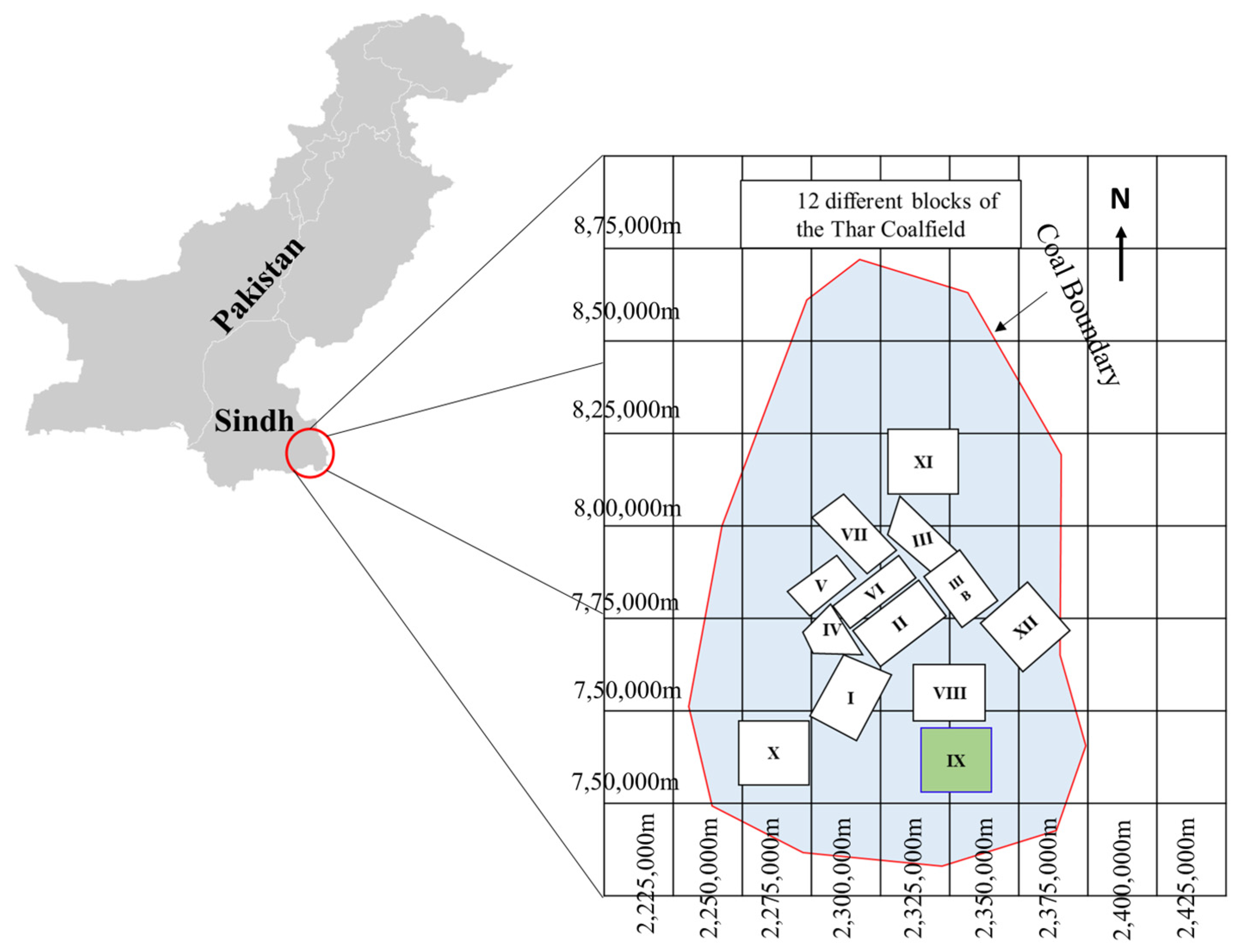
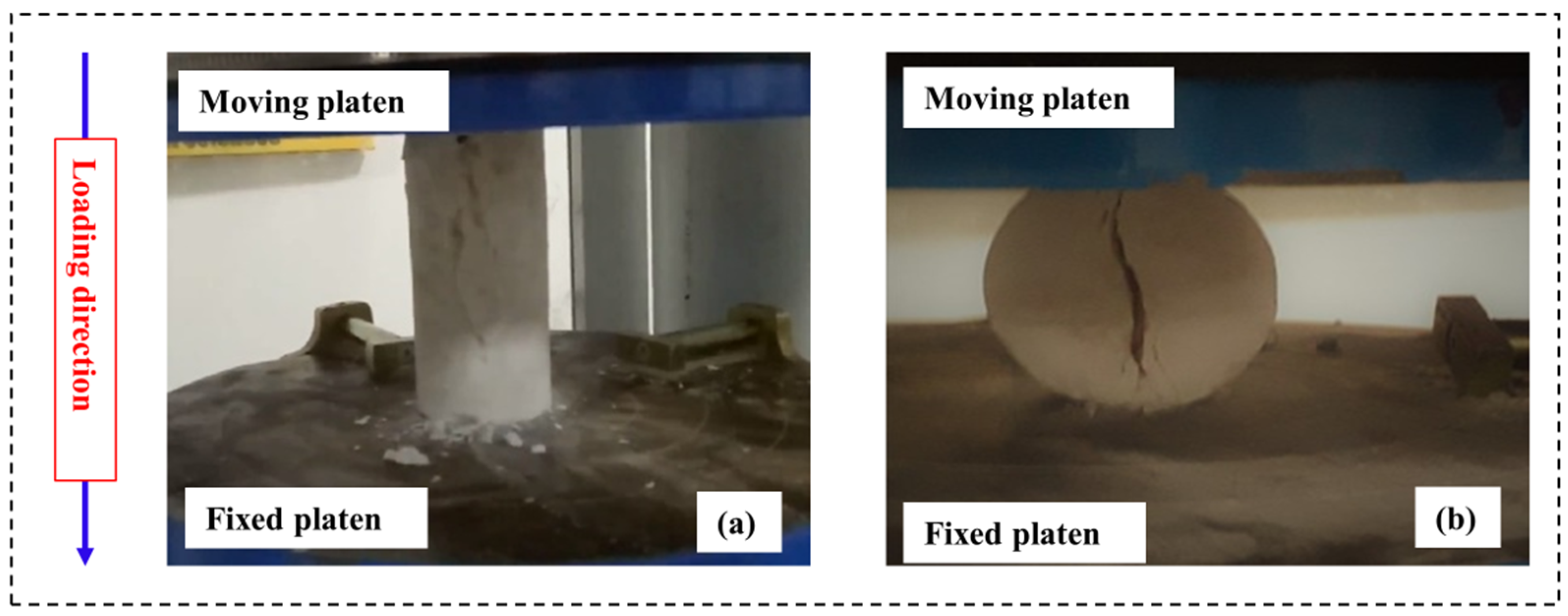
In this study, sedimentary rock samples, i.e., claystone, sandstone, and siltstone, were collected from Block IX of the Thar coalfield, Pakistan. Figure 1 represents the geological site of the collected rock samples [38]. Initially, a total of 78 core rock samples of each type were prepared and subdivided into standardized samples according to ISRM and ASTM standards to maintain the same rock core dimensions as well as geological and geotechnical features [39,40]. Next, these rock samples were tested in the laboratory at the Department of Mining Engineering, Mehran University of Engineering and Technology, to determine the physical and mechanical parameters, including ρ_d in g/cm³, BTS in MPa, ρ_wet in g/cm³, and UCS in MPa, using a universal testing machine (UTM), as shown in Figure 2a,b. Figure 2a,b represent the deformed rock core specimen for UCS and BTS tests, respectively.

Table 2. Physical and mechanical parameters of the dataset.

Dataset	ρd (g/cm3)	BTS (MPa)	ρwet (g/cm3)	UCS (MPa)
1	1.91	0.305	2.13	0.404
2	1.75	0.217	2.01	0.491
3	1.77	0.318	2.04	0.531
4	1.78	0.271	2	0.579
5	1.76	0.292	2.04	0.557
…	…	…	…	…
74	1.81	0.178	2.1	0.541
75	1.84	0.189	2.11	0.476
76	1.96	0.2	2.18	0.508
77	1.78	0.108	2.09	0.511
78	1.84	0.138	2.09	1.415

presents the five heads and five tails of the dataset of physical and mechanical parameters.

Table 3. The minimum, maximum, average, and standard deviation of the dataset.

Parameters	ρd (g/cm3)	BTS (MPa)	ρwet (g/cm3)	UCS (MPa)
Minimum	1.22	0.023	1.63	0.304
Maximum	2.12	0.627	2.3	3.55
Average	1.76	0.32	2.04	1.38
Standard deviation	0.22	0.13	0.15	0.98

shows the minimum, maximum, average, and standard deviation of parameters of rock samples determined in the laboratory.

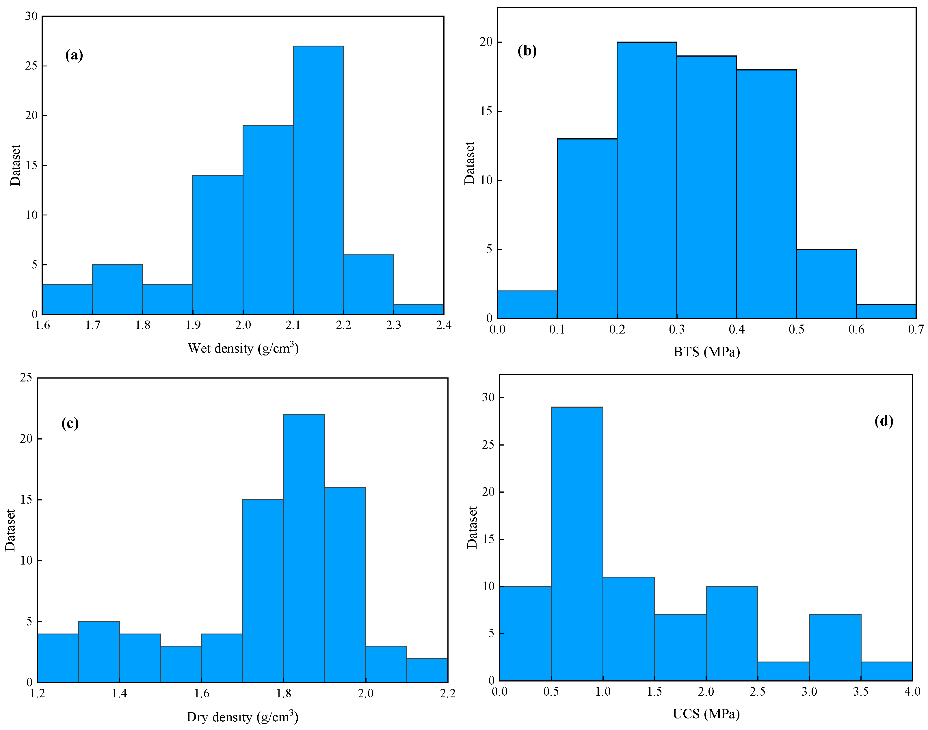
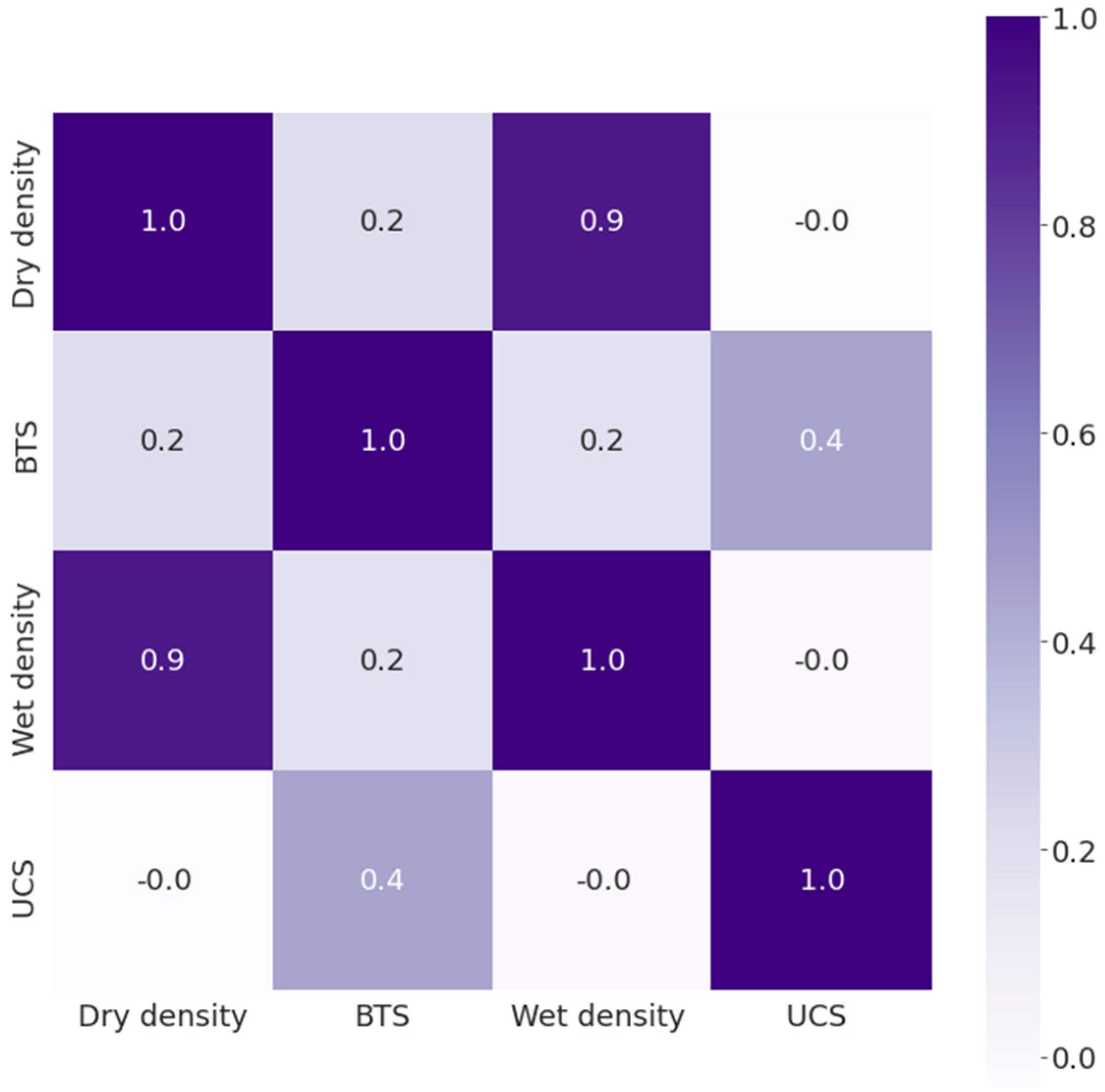
Figure 3 represents histogram plots of the original dataset in this study: (a) dry density (g/cm³), (b) BTS (MPa), (c) wet density (g/cm³), and (d) UCS (MPa). Figure 4 presents the pairwise plot of the original dataset of different parameters and UCS under this study. Notably, none of the parameters are well-correlated to the UCS, thus all of the parameters are analyzed for UCS prediction. In addition, Figure 4 represents a moderate positive correlation of BTS with UCS; however, the dry density and wet density show a negative correlation with UCS.

2.2. Methods

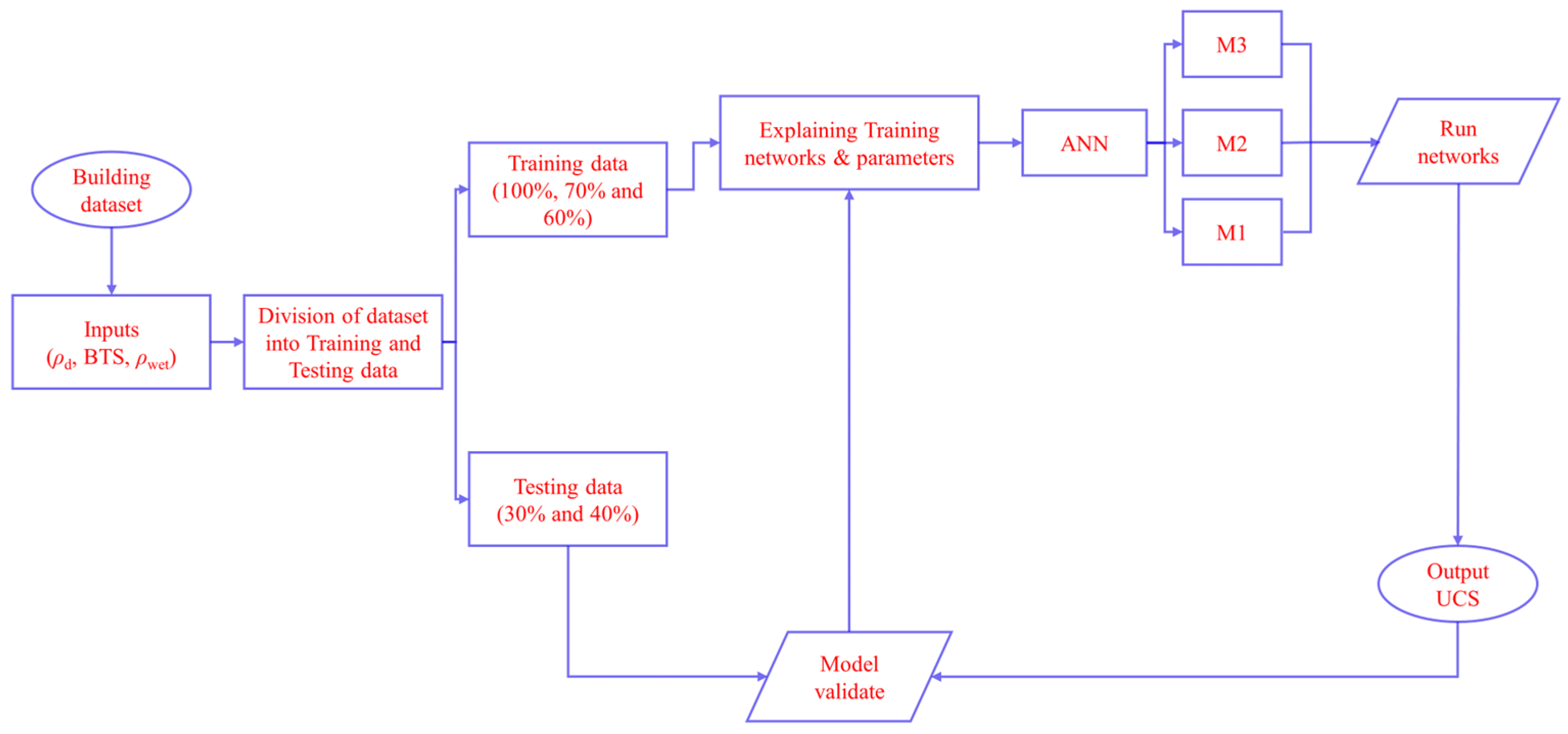
The artificial neural network (ANN) approach was employed to predict UCS with three corresponding inputs: ρ_d (g/cm³), BTS (MPa), and ρ_wet (g/cm³). Figure 5 demonstrates the flow chart of the predictive modeling process for UCS. Owing to the small number of resources available for collecting samples, the current study used a limited dataset, that is, 78 samples divided for the established models, including M1, M2, and M3, as presented in

Table 4. The dataset distribution for the ANN and MLR models.

Model Code	Dataset	Dataset Distribution (%)	Total Dataset
Model 1 (M1)	Overall	100	78
Model 2 (M2)	Train	70	55
	Test	30	23
Model 3 (M3)	Train	60	47
	Test	40	31

. M1 means the model was trained on the overall dataset, M2 means the model was trained on 70% (55 datasets) of the dataset and tested on 30% (23 datasets) of the dataset, and M3 means the model was trained on 60% (47 datasets) of the dataset and tested on 40% (31 datasets) of the dataset. In addition, Taylor diagram representation was used, which explains a brief qualitative depiction of the best fit of the model to standard deviations and correlations. Moreover, cosine amplitude method (CAM)-based sensitivity analysis was carried out in order to estimate the influence of each input variable on output UCS.

2.2.1. Artificial Neural Network

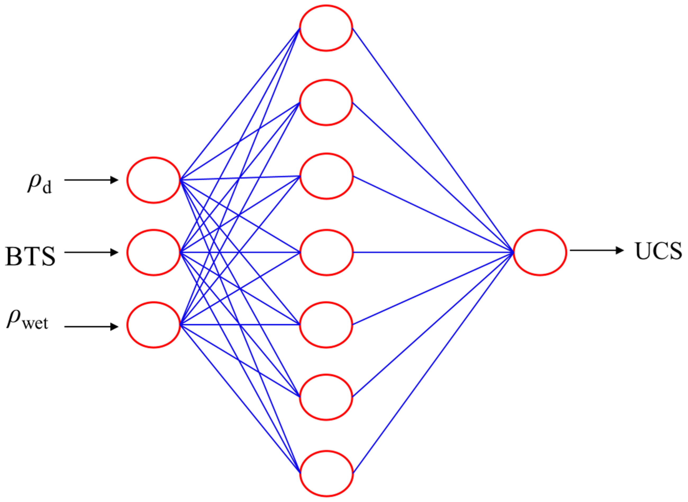
The concept of ANN was originally introduced by Frank Rosenblatt in 1958 [41]. ANN is considered to be the most common and effective soft computing technique based on the function of the human brain’s nervous system [42,43,44,45,46,47]. This technique is mainly used to solve complex rock structure design problems, i.e., mining, civil, geotechnical, geological engineering, and so on. The ANN structure is an essential factor in designing the ultimate prediction model, as the structure affects the learning capability and performance when estimating the network data. The ANN is structured with three layers (i.e., input layer, hidden layer, and output layer) with a number of interrelated units, called neurons, and the method is used to classify the appropriate correlation between the specified input and output parameters [48]. Figure 6 shows the structure of the ANN to estimate UCS in this research. Because of the complexity of the problem, each neuron has sufficient neuron capacity, and each neuron is related to the weight of the next layer [49,50,51]. Equation (1) is used to evaluate the approximate number of neurons in the hidden layer, as the improper selection of the number of neurons in the hidden layer often leads to “under-fitting” and “over-fitting” and must be avoided.

$$N_H\le 2N_1+1$$

(1)

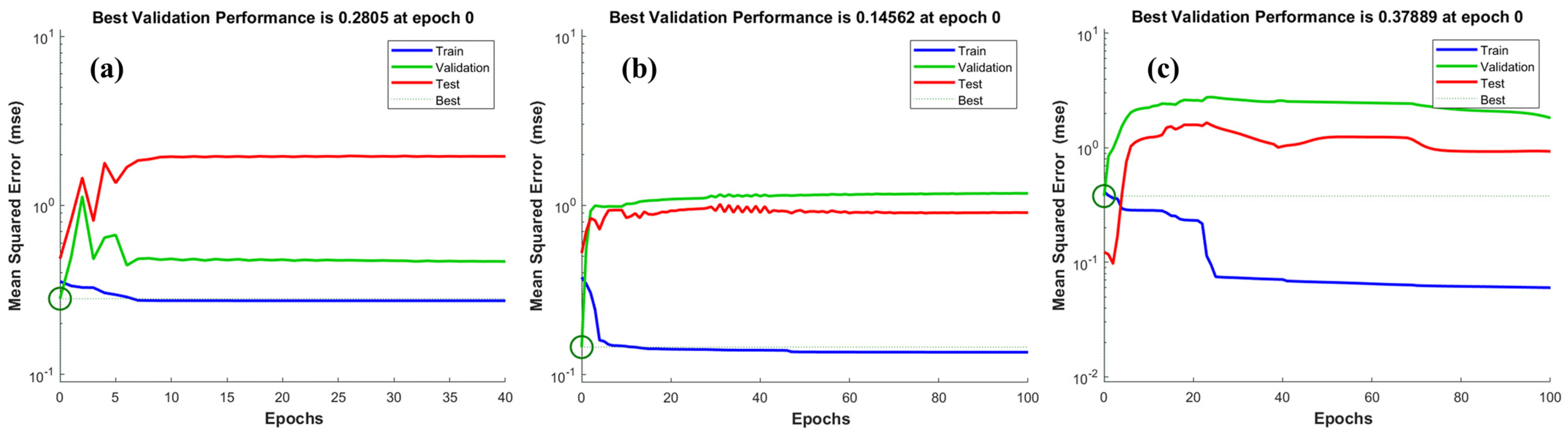
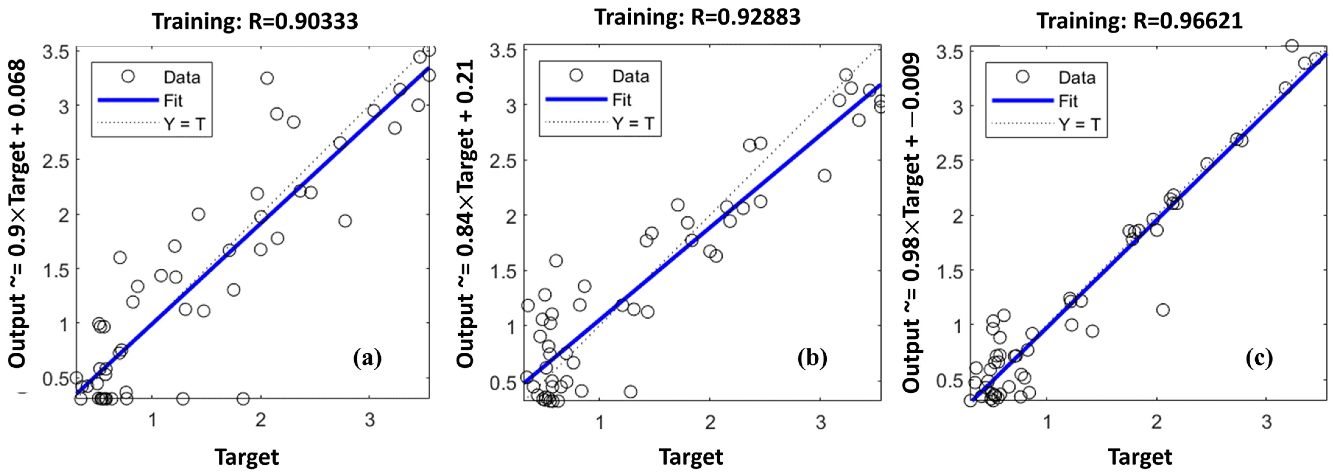
ANN toolbox in MATLAB package 2018a was used in this study to develop the feed-forward back propagation (FFBP) ANN model with 3-7-1. BP is the most commonly applied powerful learning algorithm in multilayer networks [52,53]. The predictive input parameters, ρ_d, BTS, and ρ_wet, were allocated to an input layer composed of three neurons to predict UCS of the output layer. The ANN models, M1, M2, and M3, were trained, tested, and validated. One hundred epochs were used to train the models and the minimum validation error was considered as a stopping point to prevent overfitting. Figure 7 represents the validation curves for the training performance of the ANN models of UCS. Therefore, model M2 demonstrates the best performance curve of UCS, with validation error equal to 0.14562, which is reached at 0 epochs. Figure 8 illustrates the training scatter plots of predicted UCS against measured UCS, as M1 for overall dataset and as M2 and M3 for the training and testing dataset, respectively.

2.2.2. Multiple Linear Regression

SPSS (version 23) was used to conduct a multiple linear regression (MLR) analysis to determine the existence of a linear relationship between the dependent variable and the independent variables. Regression analysis is used to determine the independent variables’ significance in determining the dependent variable’s values [54]. More precisely, the purpose of regression analysis in this study was to compare the performance of the ANN analysis to that of conventional linear regression. This approach has also been used in several recent studies on the application of ANNs and linear regression analysis [55]. The basic linear regression equation (Equation (2)), modified to include our dependent and independent variables, is as follows:

$$D=\alpha +B_1{T}_1+B_2{T}_2+B_3{T}_3+\dots B_n{T}_n+e$$

(2)

where $D$ represents the dependent variable, $\alpha$ represents the regression constant, $B$ represents the regression coefficient, and $T$ represents the value of the independent variable.

2.2.3. Model Evaluation

This study used ANN and MLR methods. To verify the prediction results of models M1, M2, and M3, the performance indices were calculated. The outcomes of all established models are illustrated as measured and predicted values. Equations (3)–(6) were used to find the coefficient of determination (R²), root mean squared error (RMSE), variance accounts for (VAF), and a20-index of each model, respectively. Table 5 represents the performance indices of the ANN and MLR models for predicting UCS on the overall dataset, training dataset, and testing dataset.

$$R^2=\frac{\sum _{i=1}^n({\mathrm{U}\mathrm{C}\mathrm{S}}_o-\stackrel{-}{{\mathrm{U}\mathrm{C}\mathrm{S}}_o})({\mathrm{U}\mathrm{C}\mathrm{S}}_p-\stackrel{-}{{\mathrm{U}\mathrm{C}\mathrm{S}}_p})}{{\sqrt{{\sum }_{i=1}^n{\left({\mathrm{U}\mathrm{C}\mathrm{S}}_o-\stackrel{-}{{\mathrm{U}\mathrm{C}\mathrm{S}}_o}\right)}^2\left({\mathrm{U}\mathrm{C}\mathrm{S}}_p-\stackrel{-}{{\mathrm{U}\mathrm{C}\mathrm{S}}_p}\right)}}^2}$$

(3)

$$RMSE=\sqrt{\frac{\sum _{i=1}^n{({\mathrm{U}\mathrm{C}\mathrm{S}}_o-{\mathrm{U}\mathrm{C}\mathrm{S}}_p)}^2}{n}}$$

(4)

$$VAF=\left[1-\frac{var({\mathrm{U}\mathrm{C}\mathrm{S}}_o-{\mathrm{U}\mathrm{C}\mathrm{S}}_p)}{var\left({\mathrm{U}\mathrm{C}\mathrm{S}}_o\right)}\right]\times 100$$

(5)

In addition, to further assess the reliability of the model, a new engineering index, a20-index, was applied to the studied models.

$$a20-index=\frac{m20}{N}$$

(6)

where ${\mathrm{U}\mathrm{C}\mathrm{S}}_o$ is the measured value; $\stackrel{-}{{\mathrm{U}\mathrm{C}\mathrm{S}}_p}$ is the predicted value; $\stackrel{-}{{\mathrm{U}\mathrm{C}\mathrm{S}}_o}$ and $\stackrel{-}{{\mathrm{U}\mathrm{C}\mathrm{S}}_p}$ are the mean of the measured and predicted value, respectively; and n shows the number of the dataset. $m20$ denotes the dataset with a value rate of measured UCS/predicted UCS between 0.80 and 1.20 and $N$ represents the dataset number.

3. Prediction and Discussion of Uniaxial Compressive Strength

The main objective of this study is to investigate the capability of an intelligent model, i.e., ANN, for predicting UCS of sedimentary rocks. The actual and predicted output values were later collated and plotted to ease the performance analysis and correlation studies of these developed models. Various analytical metrics including R², RMSE, VAF, and a20 index were used as performance criteria to examine the final output, to analyze and compare the expected models, and to evaluate the optimal model for data prediction. Model 1 (M1) is the overall dataset, model 2 (M2) consists of 70% as the training dataset and 30% as the testing dataset, and model 3 (M3) consists of 60% as the training dataset and 40% as the testing dataset.

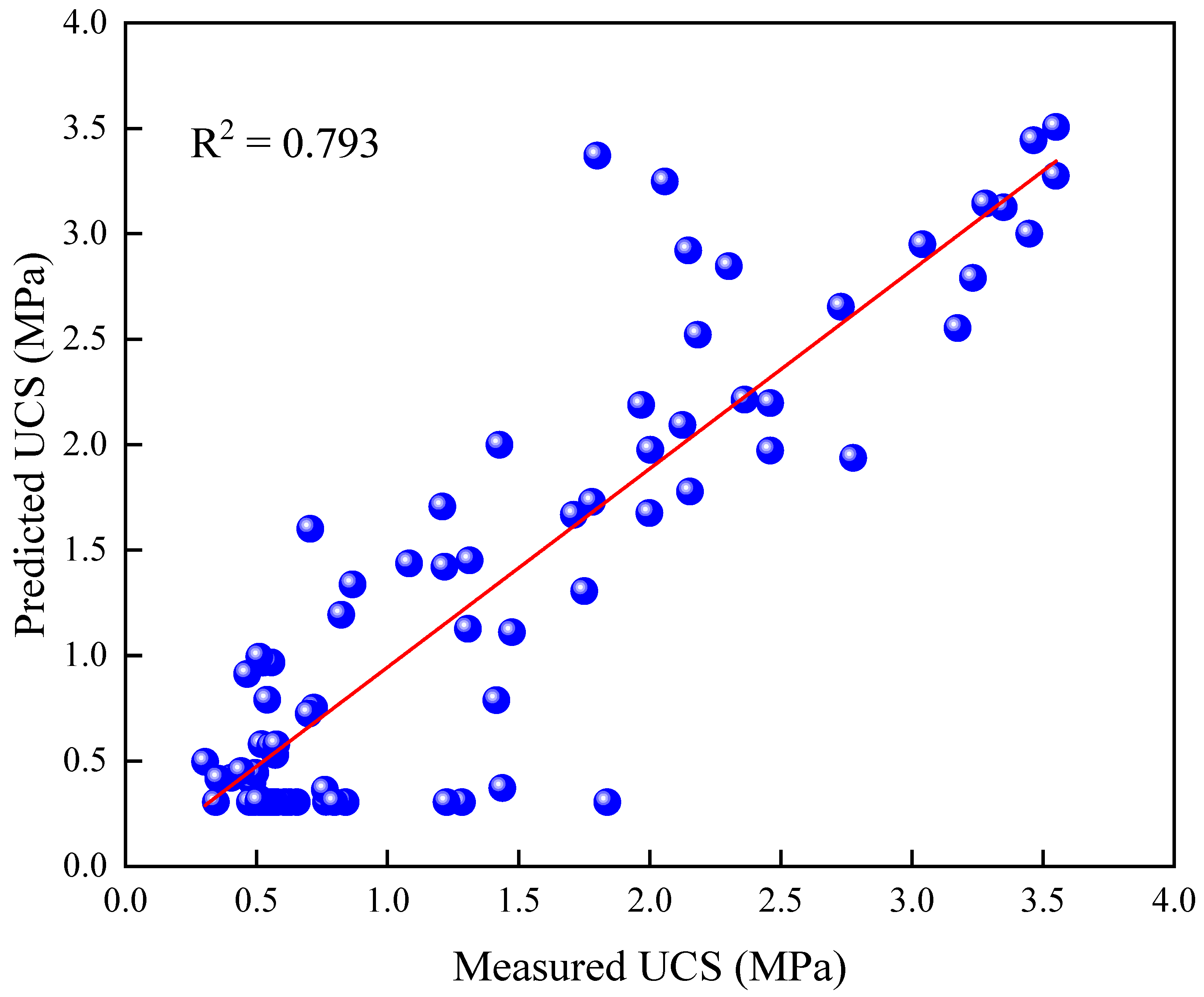
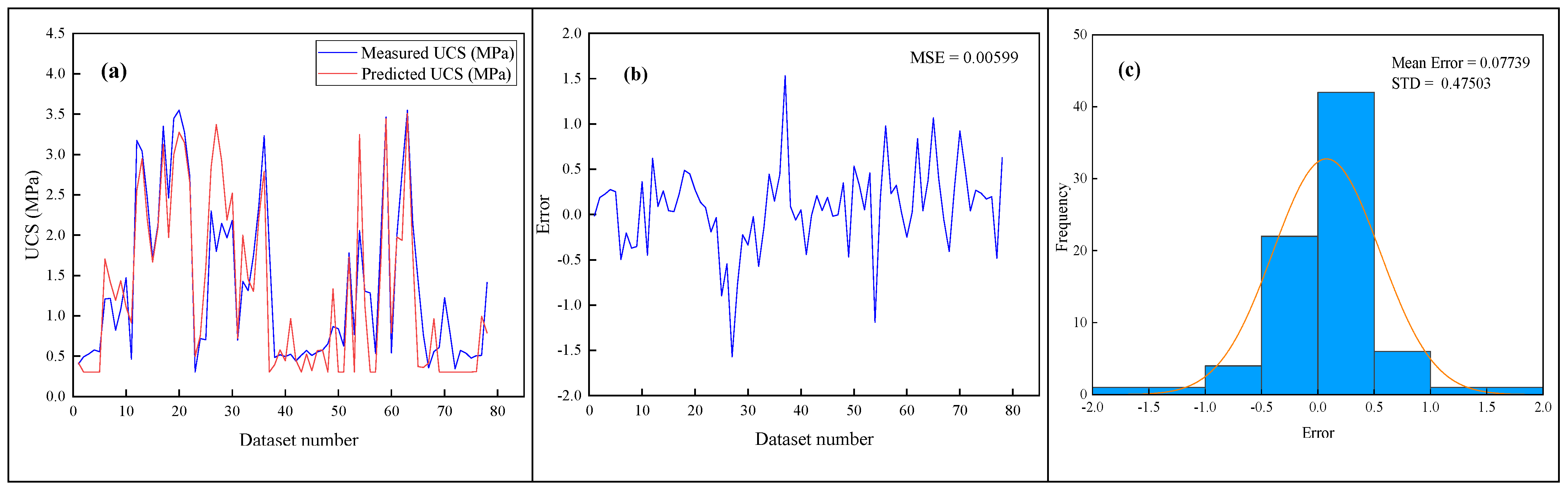
Figure 9 indicates the predicted values of the ANN model M1 for UCS against the measured UCS for the overall dataset. The predicted correlation coefficient of M1 is R² = 0.793. Based on the M1 predicted outputs, Figure 10a shows the aggregated comparison of predicted versus measured values for UCS. Figure 10b specifies the change in relative error between the measured and predicted values. The MSE value of model M1 achieved is 0.00599. Figure 10c illustrates the error histogram of the established model M1. Here, it can be considered that the distribution of the errors is approximately zero, which is in good agreement with the performance of model M1.

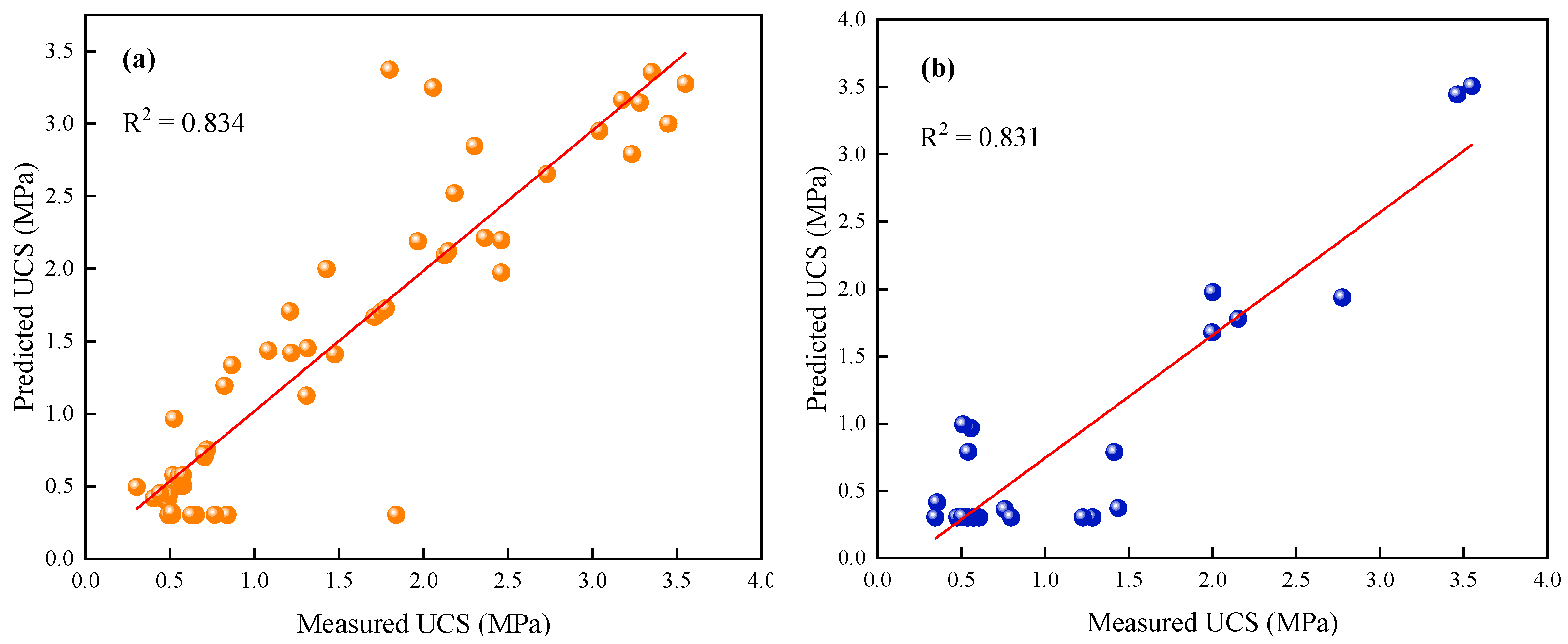
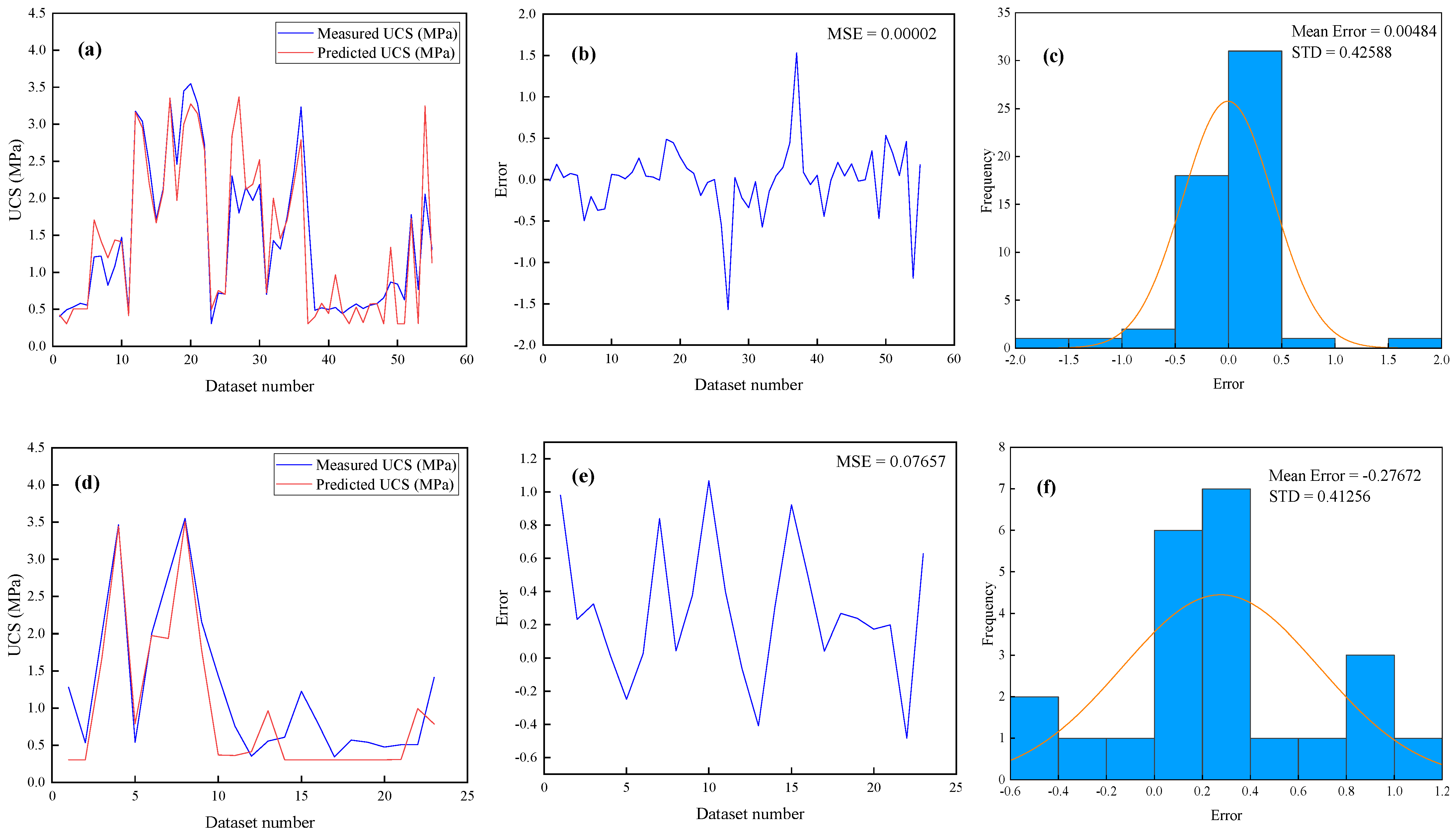
Figure 11 shows the predicted outputs of the ANN model M2 for UCS versus measured data for the training and testing data. For the training and testing data, the predicted R² values of model M2 are 0.834 and 0.831, respectively. According to the M2 estimated results for the training data, Figure 12a displays the aggregated comparison of the predicted against measured values for UCS. Figure 12b shows the change in relative error between the measured and predicted values. The MSE value of model M2 is 0.00002. Figure 12c denotes the error histogram of model M2. It can be seen that the distribution of the errors is almost zero, which indicates that the performance of the proposed model M2 is satisfactory and reliable. Similarly, Figure 12d exhibits the aggregated comparison of the predicted against measured values for UCS of estimated outputs of M3 for the testing data. Figure 12e denotes the change in relative error between the measured and predicted values. The MSE value is achieved as 0.07657. Figure 12f represents the error histogram of model M3. Consequently, it can be seen that the distribution of the errors is nearly zero, which indicates that the performance of the proposed model M2 is acceptable.

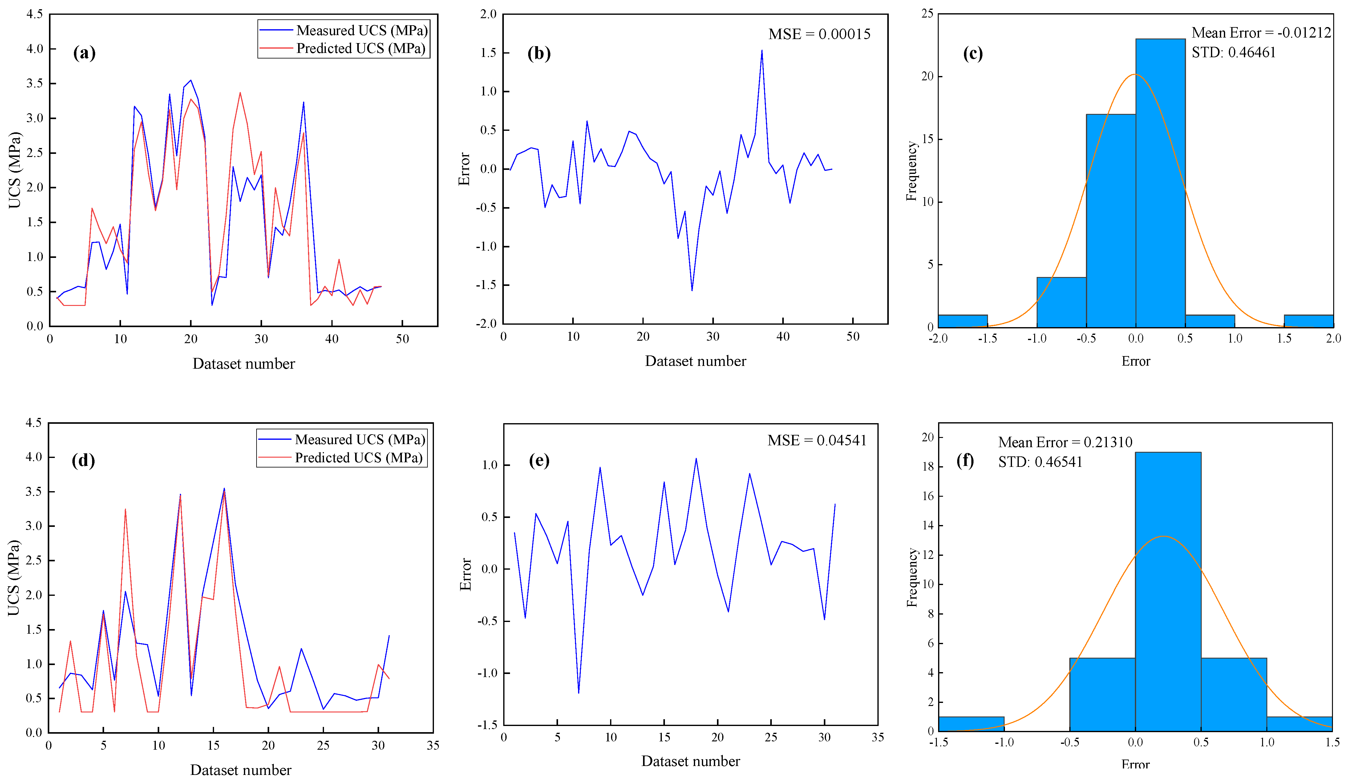
In Figure 13, the predicted outputs of the ANN model M3 for UCS versus measured data for the training and testing data are presented. Thus, the predicted R² values of model M3 are 0.807 and 0.775 for the training and testing data, respectively. Regarding the estimated results of M3 for the training data, Figure 14a shows the aggregated comparison of the predicted against measured values of UCS. Figure 14b shows the change in relative error between the measured and predicted values. The MSE value of M3 is 0.00015. Figure 14c signifies the error histogram of the developed model M3. Hence, it can be noted that the error distribution approaches zero, which shows that the performance of model M3 is adequate. Likewise, for predictive outputs of M3 for the testing data, Figure 14d reveals the aggregated comparison of the predicted against measured values for UCS. Figure 14e indicates the change in relative error between the measured and predicted values. The MSE value of M3 is 0.04541. Figure 14f presents the error histogram of model M3. Thus, the distribution of the errors is nearly zero, which indicates that the performance of the established model M3 is satisfactory.

The first step is to determine whether the data under consideration are appropriate for linear regression analysis. Numerous tests are suggested in the literature for this purpose. Apart from R², another very commonly used test is the ANOVA test. In the first case, linear regression was used to determine the relationship between the dependent variable measured UCS and the three independent variables: ${\rho }_{\mathrm{d}}$, BTS, and ${\rho }_{\mathrm{w}\mathrm{e}\mathrm{t}}$. In Table 6, the R² values of UCS are estimated using different equations of the MLR models, including M1, M2, and M3, for the overall dataset and training and testing data, i.e., 0.187 for M1, 0.292 and 0.066 for M2, and 0.425 and 0.062 for M3, respectively. Therefore, the R² values of UCS are quite satisfactory in models M1, M2, and M2. Furthermore, the ANOVA test also rejected the null hypothesis at a significance value of p < 0.001.

Table 5. Performance indices of the ANN and MLR models for predicting UCS for the overall dataset, training dataset, and testing dataset.

Model			UCS
			R2	RMSE	VAF (%)	a20-index
ANN	M1	Overall dataset	0.793	0.07739	0.96	0.95
	M2	Train	0.834	0.00484	0.99	0.99
		Test	0.831	0.27672	0.92	0.80
	M3	Train	0.807	0.01211	0.99	0.99
		Test	0.775	0.21311	0.90	0.80
MLR	M1	Overall dataset	0.187	6.70404	0.98	1.07
	M2	Train	0.292	3.33067	0.77	0.80
		Test	0.066	1.40950	0.81	0.99
	M3	Train	0.425	1.32518	0.82	1.05
		Test	0.062	7.12692	0.99	0.99

Table 5. Performance indices of the ANN and MLR models for predicting UCS for the overall dataset, training dataset, and testing dataset.

Model			UCS
			R2	RMSE	VAF (%)	a20-index
ANN	M1	Overall dataset	0.793	0.07739	0.96	0.95
	M2	Train	0.834	0.00484	0.99	0.99
		Test	0.831	0.27672	0.92	0.80
	M3	Train	0.807	0.01211	0.99	0.99
		Test	0.775	0.21311	0.90	0.80
MLR	M1	Overall dataset	0.187	6.70404	0.98	1.07
	M2	Train	0.292	3.33067	0.77	0.80
		Test	0.066	1.40950	0.81	0.99
	M3	Train	0.425	1.32518	0.82	1.05
		Test	0.062	7.12692	0.99	0.99

Table 6. Multiple linear regression analysis for UCS in MPa; ${\rho }_d$ (g/cm³), BTS (MPa), and ${\rho }_{wet}$ (g/cm³) are the dry density, Brazilian tensile strength, and wet density, respectively.

Model Code	Dataset	Equation	R2
M1	Overall	$\mathrm{U}\mathrm{C}\mathrm{S}=1.49-0.93{\rho }_d+3.12\mathrm{B}\mathrm{T}\mathrm{S}+0.26{\rho }_{wet}$	0.187
M2	Train	$\mathrm{U}\mathrm{C}\mathrm{S}=1.04-1.11{\rho }_d+4.35\mathrm{B}\mathrm{T}\mathrm{S}+0.41{\rho }_{wet}$	0.292
	Test	$\mathrm{U}\mathrm{C}\mathrm{S}=7.83-7.24{\rho }_{wet}+4.61{\rho }_d+0.80\mathrm{B}\mathrm{T}\mathrm{S}$	0.066
M3	Train	$\mathrm{U}\mathrm{C}\mathrm{S}=0.72-1.80{\rho }_d+0.80{\rho }_{wet}+6.17\mathrm{B}\mathrm{T}\mathrm{S}$	0.425
	Test	$\mathrm{U}\mathrm{C}\mathrm{S}=0.59-4.05{\rho }_{wet}+4.90{\rho }_d+0.24\mathrm{B}\mathrm{T}\mathrm{S}$	0.062

Table 6. Multiple linear regression analysis for UCS in MPa; ${\rho }_d$ (g/cm³), BTS (MPa), and ${\rho }_{wet}$ (g/cm³) are the dry density, Brazilian tensile strength, and wet density, respectively.

Model Code	Dataset	Equation	R2
M1	Overall	$\mathrm{U}\mathrm{C}\mathrm{S}=1.49-0.93{\rho }_d+3.12\mathrm{B}\mathrm{T}\mathrm{S}+0.26{\rho }_{wet}$	0.187
M2	Train	$\mathrm{U}\mathrm{C}\mathrm{S}=1.04-1.11{\rho }_d+4.35\mathrm{B}\mathrm{T}\mathrm{S}+0.41{\rho }_{wet}$	0.292
	Test	$\mathrm{U}\mathrm{C}\mathrm{S}=7.83-7.24{\rho }_{wet}+4.61{\rho }_d+0.80\mathrm{B}\mathrm{T}\mathrm{S}$	0.066
M3	Train	$\mathrm{U}\mathrm{C}\mathrm{S}=0.72-1.80{\rho }_d+0.80{\rho }_{wet}+6.17\mathrm{B}\mathrm{T}\mathrm{S}$	0.425
	Test	$\mathrm{U}\mathrm{C}\mathrm{S}=0.59-4.05{\rho }_{wet}+4.90{\rho }_d+0.24\mathrm{B}\mathrm{T}\mathrm{S}$	0.062

Taylor Diagram

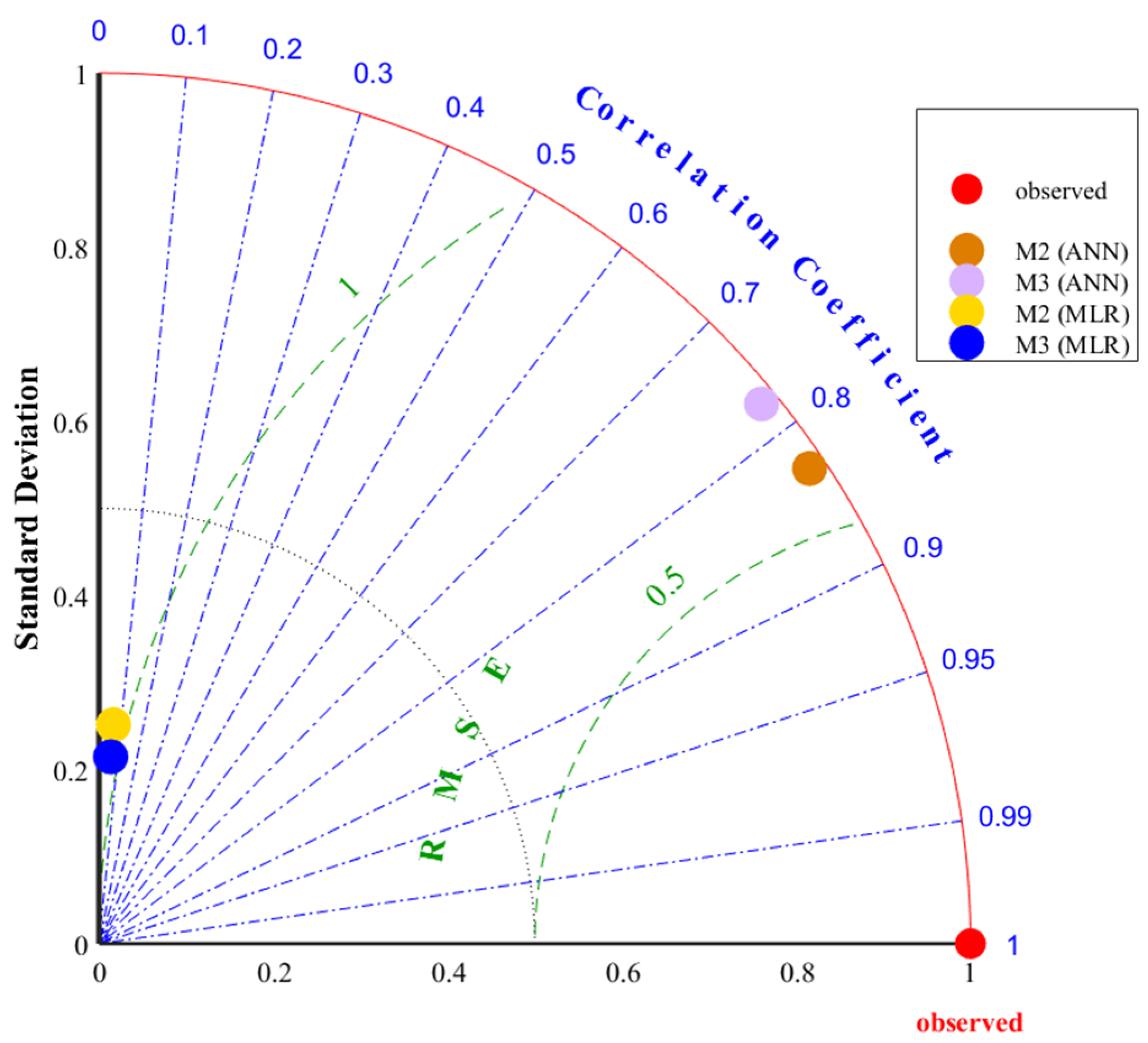
The Taylor diagram provides a short numerical explanation of how the fit patterns match their connection and standard deviation. The Taylor diagram can be expressed as follows:

$$R=\frac{\frac{1}{Z}{\sum }_z^Z(l_n-\stackrel{-}{l})(m_n-\stackrel{-}{m})}{{\sigma }_l{\sigma }_m}$$

(7)

where R denotes the correlation; Z denotes the discrete points; $l_n$ and $m_n$ represent two variables; ${\sigma }_l$ and ${\sigma }_m$ show the standard deviation of l and m, respectively; and $\stackrel{-}{l}$ and $\stackrel{-}{m}$ denote the average of ${\sigma }_l$ and ${\sigma }_m$, respectively.

Figure 15 indicates the Taylor diagrammatic correlation between the R², RMSE, and standard deviation of the original and predicted UCS for the M2 and M3 ANN and MLR models for the testing stage. The prediction of ANN model M3 is highly correlated with the original values and, compared with the other developed models, the standard deviation is similar to the original value. Thus, ANN model M2 with R² = 0.831 is the most suitable for predicting UCS of sedimentary rocks in the Thar coalfield, Pakistan, among the developed models.

In an ideal scenario, the best-fit prediction model is considered as the one in which the R² value is highest, the RMSE is lowest, the VAF is at a maximum, and the a20-index is reliable. Therefore, according to Figure 15, ANN model M2 for the testing dataset revealed the optimal results and is proposed as the best-fit prediction model for UCS in this study.

4. Sensitivity Analysis

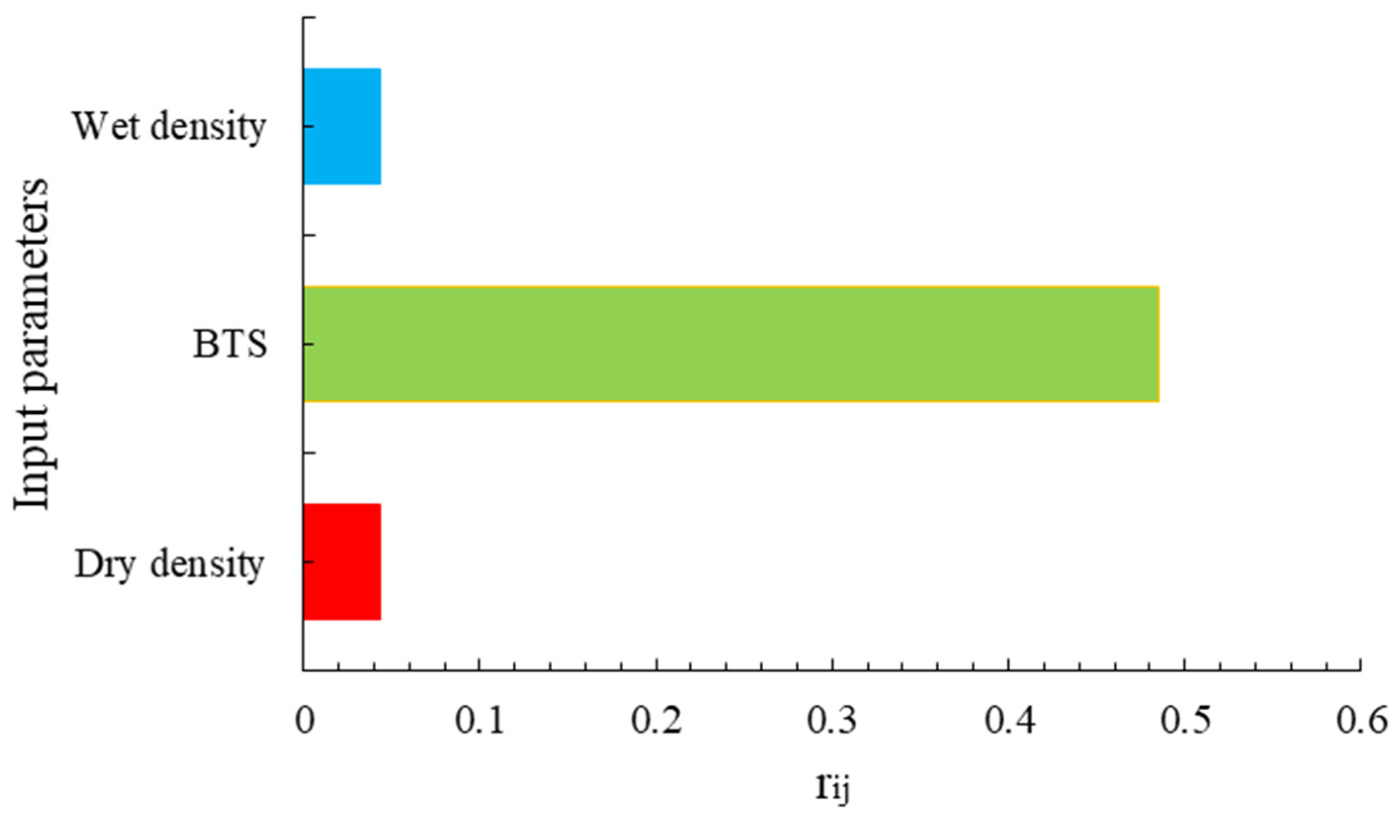
It is crucial to accurately analyze the most important parameters that have a great influence on UCS of rock, which can certainly be problematic in the design of structures. Therefore, in this study, the cosine amplitude method was used to investigate the relative influence of the input parameters on the output [56,57]. The general formula of the adopted method can be expressed as follows:

$$r_{ij}=\frac{\sum _{k=1}^n{(\mathrm{U}\mathrm{C}\mathrm{S}}_{ik}{\mathrm{U}\mathrm{C}\mathrm{S}}_{jk})}{\sqrt{{\sum }_{k=1}^n{\mathrm{U}\mathrm{C}\mathrm{S}}_{ik}^2{\sum }_{k=1}^n{\mathrm{U}\mathrm{C}\mathrm{S}}_{jk}^2}}$$

(8)

where ${\mathrm{U}\mathrm{C}\mathrm{S}}_i$ and ${\mathrm{U}\mathrm{C}\mathrm{S}}_j$ are input and output values, respectively, and n denotes the dataset number during the testing stage. Finally, $r_{ij}$ ranges between 0 and 1, specifying additional evidence of the accuracy between each variable and the target. According to Equation (6), if the $r_{ij}$ of any parameter is 0, this indicates that there is no significant relationship between this parameter and the target. On the contrary, when $r_{ij}$ is equal to 1 or approximately 1, a significant relationship can be considered that can greatly influence UCS of the rocks.

Figure 16 shows the relationship between each input parameter (${\rho }_{\mathrm{d}}$, BTS, and ${\rho }_{\mathrm{w}\mathrm{e}\mathrm{t}}$) of the developed model and the output (UCS). Therefore, it can be seen from the figure that BTS is the most influential parameter in predicting UCS. The corresponding coefficient values are ${\rho }_{\mathrm{d}}$ = 0.0437, BTS = 0.485, and ${\rho }_{\mathrm{w}\mathrm{e}\mathrm{t}}$ = 0.0435.

5. Conclusions

In this study, an intelligent method was used to predict the output, UCS, of sedimentary rocks collected from Block IX of the Thar coalfield, using ρ_d, BTS, and ρ_wet as input parameters. The physical and mechanical properties of rock samples were determined in a laboratory in accordance with ISRM and ASTM standards. This study determined the predictive performance of ANN and MLR models by determining the highest R², the smallest RMSE, the highest VAF, and a reliable a20-index as follows:

For ANN models, R², RMSE, VAF, and a20-index were 0.793, 0.07739, 0.96, and 0.95, respectively, for M1; 0.834 and 0.831, 0.00484 and 0.27672, 0.99 and 0.92, and 0.99 and 0.80, respectively, for the training and testing dataset of M2; and 0.807 and 0.775, 0.01211 and 0.21311, 0.99 and 0.90, and 0.99 and 0.80, respectively, for the training and testing dataset of M3.

In comparison, for the MLR models, R², RMSE, VAF, and a20-index were 0.187, 6.70404, 0.98, and 1.07, respectively, for M1; 0.292 and 0.066, 3.33067 and 1.40950, 0.77 and 0.81, and 0.80 and 0.99, respectively, for the training and testing dataset of M2; and 0.425 and 0.062, 1.32518 and 7.12692, 0.82 and 0.99, and 1.05 and 0.99, respectively, for the training and testing dataset of M3.

Thus, the proposed ANN model M2 for the testing dataset yielded the optimal results and is proposed as the best-fit prediction model for UCS in this study.

Finally, by performing a sensitivity analysis, it was concluded that BTS was the most influential parameter in predicting UCS.

The current study used only ANN to predict UCS, in comparison with MLR, which could have produced more suitable results. However, future work will focus on predicting UCS using metaheuristic techniques and enhancing the accuracy of the model prediction and model performance in heterogeneous and big datasets. Moreover, the author plans to investigate UCS using optimized machine learning algorithms as well as hybrid and ensemble learning. Furthermore, some other influential attributes will be added to the UCS database to further understand the nature of this study area.

References

- Madhubabu, N.; Singh, P.K.; Kainthola, A.; Mahanta, B.; Tripathy, A.; Singh, T.N. Prediction of compressive strength and elastic modulus of carbonate rocks. Measurement 2016, 88, 202–213. [Google Scholar] [CrossRef]
- Asheghi, R.; Shahri, A.A.; Zak, M.K. Prediction of uniaxial compressive strength of different quarried rocks using metaheuristic algorithm. Arab. J. Sci. Eng. 2019, 44, 8645–8659. [Google Scholar] [CrossRef]
- Abdi, Y.; Taheri-Garavand, A. Application of the ANFIS Approach for Estimating the Mechanical Properties of Sandstones. Emir. J. Eng. Res. 2020, 25, 1. [Google Scholar]
- Abdi, Y.; Garavand, A.T.; Sahamieh, R.Z. Prediction of strength parameters of sedimentary rocks using artificial neural networks and regression analysis. Arab. J. Geosci. 2018, 11, 587. [Google Scholar] [CrossRef]
- Shahri, A.A.; Asheghi, R.; Zak, M.K. A hybridized intelligence model to improve the predictability level of strength index parameters of rocks. Neural Comput. Appl. 2020, 33, 3841–3854. [Google Scholar] [CrossRef]
- Barzegar, R.; Sattarpour, M.; Deo, R.; Fijani, E.; Adamowski, J. An ensemble tree-based machine learning model for predicting the uniaxial compressive strength of travertine rocks. Neural Comput. Appl. 2019, 32, 9065–9080. [Google Scholar] [CrossRef]
- Gockceoglu, C.; Zorlu, K. A fuzzy model to predict the uniaxial compressive strength and the modulus of elasticity of a problematic rock. Eng. Appl. Artif. Intell. 2004, 17, 61–72. [Google Scholar] [CrossRef]
- Baykasoğlu, A.; Gϋllϋ, H.; Ҫanakҫi, A.; Ӧzbakir, A. Predicting of compressive and tensile strength of limestone via genetic programming. Expert Syst. Appl. 2008, 35, 111–112. [Google Scholar] [CrossRef]
- Tiryaki, B. Predicting intact rock strength for mechanical excavation using multivariate statistics, artificial neural networks and regression trees. Eng. Geol. 2008, 99, 51–60. [Google Scholar] [CrossRef]
- Ozcelik, Y.; Bayram, F.; Yasitli, N.E. Prediction of engineering properties of rocks from microscopic data. Arab. J. Geosci. 2013, 6, 3651–3668. [Google Scholar] [CrossRef]
- Rajesh-Kumar, B.; Vardhan, H.; Govindaraj, M.; Vijay, G.S. Regression analysis and ANN models to predict rock properties from sound levels produced during drilling. Int. J. Rock Mech. Min. Sci. 2013, 58, 61–72. [Google Scholar] [CrossRef]
- Kong, F.; Shang, J. A validation study for the estimation of uniaxial compressive strength based on index tests. Rock Mech. Rock Eng. 2018, 51, 2289–2297. [Google Scholar] [CrossRef]
- Teymen, A.; Mengüç, E.C. Comparative evaluation of different statistical tools for the prediction of uniaxial compressive strength of rocks. Int. J. Min. Sci. Technol. 2020, 30, 785–797. [Google Scholar] [CrossRef]
- Ajalloeian, R.; Kamani, M. An investigation of the relationship between Los Angeles abrasion loss and rock texture for carbonate aggregates. Bull. Eng. Geol. Env. 2019, 78, 1555–1563. [Google Scholar] [CrossRef]
- Cabalar, A.F.; Cevik, A.; Gokceoglu, C. Some applications of Adaptive Neuro-Fuzzy Inference System (ANFIS) in geotechnical engineering. Comput. Geotech. 2012, 40, 14–33. [Google Scholar] [CrossRef]
- Bashari, A.; Beiki, M.; Talebinejad, A. Estimation of deformation modulus of rock masses by sing fuzzy clustering-based modeling. Int. J. Rock Mech. Min. Sci. 2011, 48, 1224–1234. [Google Scholar] [CrossRef]
- Umrao, R.K.; Sharma, L.K.; Singh, R.; Singh, T.N. Determination of strength and modulus of elasticity of heterogenous sedimentary rocks: An ANFIS predictive technique. Measurement 2018, 126, 194–201. [Google Scholar] [CrossRef]
- Torabi-Kaveh, M.; Naseri, F.; Saneie, S.; Sarshari, B. Application of artificial neural networks and multivariate statistics to predict UCS and E using physical properties of Asmari limestones. Arab. J. Geosci. 2015, 8, 2889–2897. [Google Scholar] [CrossRef]
- Yagiz, S.; Sezer, E.A.; Gokceoglu, C. Artificial neural networks and nonlinear regression techniques to assess the influence of slake durability cycles on the prediction of uniaxial compressive strength and modulus of elasticity for carbonate rocks. Int. J. Numer. Anal. Methods Geomech. 2012, 36, 1636–1650. [Google Scholar] [CrossRef]
- Ceryan, N.; Okkan, U.; Kesimal, A. Prediction of unconfined compressive strength of carbonate rocks using artificial neural networks. Environ. Earth Sci. 2013, 68, 807–819. [Google Scholar] [CrossRef]
- Mohamad, E.T.; Armaghani, D.J.; Momeni, E.; Abad, S.V.A.N.K. Prediction of the unconfined compressive strength of soft rocks: A PSO-based ANN approach. Bull. Eng. Geol. Environ. 2015, 74, 745–757. [Google Scholar] [CrossRef]
- Aboutaleb, S.; Behnia, M.; Bagherpour, R.; Bluekian, B. Using non-destructive tests for estimating uniaxial compressive strength and static Young’s modulus of carbonate rocks via some modeling techniques. Bull. Eng. Geol. Environ. 2018, 77, 1717–1728. [Google Scholar] [CrossRef]
- Bejarbaneh, B.Y.; Bejarbaneh, E.Y.; Fahimifar, A.; Armaghani, D.J.; Abd Majid, M.Z. Intelligent modelling of sandstone deformation behaviour using fuzzy logic and neural network systems. Bull. Eng. Geol. Environ. 2018, 77, 345–361. [Google Scholar] [CrossRef]
- Fakir, M.; Ferentinou, M.; Misra, S. An investigation into the rock properties influencing the strength in some granitoid rocks of KwaZulu-Natal, South Africa. Geotech. Geol. Eng. 2017, 35, 1119–1140. [Google Scholar] [CrossRef]
- Han, H.; Yin, S. In-situ stress inversion in Liard Basin, Canada, from caliper logs. Petroleum 2020, 6, 392–403. [Google Scholar] [CrossRef]
- Skentou, A.D.; Bardhan, A.; Mamou, A.; Lemonis, M.E.; Kumar, G.; Samui, P.; Armaghani, D.J.; Asteris, P.G. Closed-Form Equation for Estimating Unconfined Compressive Strength of Granite from Three Non-destructive Tests Using Soft Computing Models. Rock Mech. Rock Eng. 2022, 11, 487–514. [Google Scholar] [CrossRef]
- Kaloop, M.R.; Bardhan, A.; Samui, P.; Hu, J.W.; Zarzoura, F. Computational intelligence approaches for estimating the unconfined compressive strength of rocks. Arab. J. Geosci. 2023, 16, 37. [Google Scholar] [CrossRef]
- Xiang, Z.; Yu, Z.; Kang, W.H.; Si, G.; Oh, J.; Canbulat, I. Estimation of in-situ rock strength from borehole geophysical logs in Australian coal mine sites. Int. J. Coal Geol. 2023, 269, 104210. [Google Scholar] [CrossRef]
- Köken, E.; Koca, T.K. A comparative study to estimate the mode I fracture toughness of rocks using several soft computing techniques. Turk. J. Eng. 2023, 7, 296–305. [Google Scholar] [CrossRef]
- Li, D.; Armaghani, D.J.; Zhou, J.; Lai, S.H.; Hasanipanah, M. A GMDH predictive model to predict rock material strength using three non-destructive tests. J. Nondestruct. Eval. 2020, 39, 81. [Google Scholar] [CrossRef]
- Dehghan, S.; Sattari, G.H.; Chelgani, S.C.; Aliabadi, M.A. Prediction of uniaxial compressive strength and modulus of elasticity for Travertine samples using regression and artificial neural networks. Min. Sci. Technol. 2010, 20, 41–46. [Google Scholar] [CrossRef]
- Yesiloglu-Gultekin, N.; Gokceoglu, C.; Sezer, E.A. Prediction of uniaxial compressive strength of granitic rocks by various nonlinear tools and comparison of their performances. Int. J. Rock Mech. Min. Sci. 2013, 62, 113–122. [Google Scholar] [CrossRef]
- Mohamad, E.T.; Armaghani, D.J.; Momeni, E.; Yazdavar, A.H.; Ebrahimi, M. Rock strength estimation: A PSO-based BP approach. Neural Comput. Appl. 2018, 30, 1635–1646. [Google Scholar] [CrossRef]
- Armaghani, D.J.; Amin, M.F.M.; Yagiz, S.; Faradonbeh, R.S.; Abdullah, R.A. Prediction of the uniaxial compressive strength of sandstone using various modeling techniques. Int. J. Rock Mech. Min. Sci. 2016, 85, 174–186. [Google Scholar] [CrossRef]
- Armaghani, D.J.; Mohamad, E.T.; Momeni, E.; Monjezi, M.; Narayanasamy, M.S. Prediction of the strength and elasticity modulus of granite through an expert artificial neural network. Arab. J. Geosci. 2016, 9, 48. [Google Scholar] [CrossRef]
- Heidari, M.; Mohseni, H.; Jalali, S.H. Prediction of uniaxial compressive strength of some sedimentary rocks by fuzzy and regression models. Geotech. Geol. Eng. 2018, 36, 401–412. [Google Scholar] [CrossRef]
- Yılmaz, I.; Yuksek, A.G. An example of artificial neural network (ANN) application for indirect estimation of rock parameters. Rock Mech. Rock Eng. 2008, 41, 781–795. [Google Scholar] [CrossRef]
- Shahani, N.M.; Zheng, X.; Guo, X.; Wei, X. MachineLearning-Based Intelligent Predictionof Elastic Modulus of Rocks at Thar Coalfield. Sustainability 2022, 14, 3689. [Google Scholar] [CrossRef]
- Brown, E.T. Rock Characterization Testing & Monitoring—ISRM Suggested Methods; ISRM—International Society for Rock Mechanics/Pergamon Press: London, UK, 2007; p. 211. [Google Scholar]
- ASTM—American Society for Tenting and Materials. Standard Practices for Preparing Rock Core as Cylindrical Test Specimens and Verifying Conformance to Dimensionaland Shape Tolerances; ASTM: West Conshohocken, PA, USA, 2013. [Google Scholar]
- Alexx, K. Artificial Neural Networks. Available online: https://www.computerworld.com/article/2591759/artificial-neural-networks.html#:~:text=One%20answer%20is%20to%20use,and%20learned%20to%20recognize%20objects (accessed on 3 July 2021).
- Alizadeh, M.; Alizadeh, E.; Asadollahpour Kotenaee, S.; Shahabi, H.; Beiranvand Pour, A.; Panahi, M.; Bin Ahmad, B.; Saro, L. Social vulnerability assessment using artificial neural network (ANN) model for earthquake hazard in Tabriz city, Iran. Sustainability 2018, 10, 3376. [Google Scholar] [CrossRef] [Green Version]
- Asteris, P.G.; Mokos, V.G. Concrete compressive strength using artificial neural networks. Neural Comput. Appl. 2019, 32, 11807–11826. [Google Scholar] [CrossRef]
- Pham, B.T.; Singh, S.K.; Ly, H.B. Using Artificial Neural Network (ANN) for prediction of soil coefficient of consolidation. Vietnam J. Earth Sci. 2020, 42, 311–319. [Google Scholar] [CrossRef]
- Pham, T.A.; Ly, H.B.; Tran, V.Q.; Giap, L.V.; Vu, H.L.T.; Duong, H.A.T. Prediction of pile axial bearing capacity using artificial neural network and random forest. Appl. Sci. 2020, 10, 1871. [Google Scholar] [CrossRef] [Green Version]
- Le, V.M.; Pham, B.T.; Le, T.T.; Ly, H.B.; Le, L.M. Daily rainfall prediction using nonlinear autoregressive neural network. Micro-Electron. Telecommun. Eng. 2020, 106, 213–221. [Google Scholar]
- Le, T.T.; Pham, B.T.; Le, V.M.; Ly, H.B.; Le, L.M. A robustness analysis of different nonlinear autoregressive networks using Monte Carlo simulations for predicting high fluctuation rainfall. Micro-Electron. Telecommun. Eng. 2020, 106, 205–212. [Google Scholar]
- Ly, H.B.; Le, T.T.; Vu, H.L.T.; Tran, V.Q.; Le, L.M.; Pham, B.T. Computational hybrid machine learning based prediction of shear capacity for steel fiber reinforced concrete beams. Sustainability 2020, 12, 2709. [Google Scholar] [CrossRef] [Green Version]
- Rashidian, V.; Hassanlourad, M. Application of an artificial neural network for modeling the mechanical behavior of carbonate soils. Int. J. Geomech. 2014, 14, 142–150. [Google Scholar] [CrossRef]
- Fidan, S.; Oktay, H.; Polat, S.; Ozturk, S. An artificial neural network model to predict the thermal properties of concrete using different neurons and activation functions. Adv. Mater. Sci. Eng. 2019, 2019, 3831813. [Google Scholar] [CrossRef] [Green Version]
- Gowida, A.; Moussa, T.; Elkatatny, S.; Ali, A. A hybrid artificial intelligence model to predict the elastic behavior of sandstone rocks. Sustainability 2019, 11, 5283. [Google Scholar] [CrossRef] [Green Version]
- Hajihassani, M.; Armaghani, D.J.; Sohaei, H.; Mohamad, E.T.; Marto, A. Prediction of airblast-overpressure induced by blasting using a hybrid artificial neural network and particle swarm optimization. Appl. Acoust. 2014, 80, 57–67. [Google Scholar] [CrossRef]
- Ekemen Keskin, T.; Özler, E.; Şander, E.; Düğenci, M.; Ahmed, M.Y. Prediction of electrical conductivity using ANN and MLR: A case study from Turkey. Acta Geophys. 2020, 68, 811–820. [Google Scholar] [CrossRef]
- Sajid, M.J. Modelling best fit-curve between China’s production and consumption-based temporal carbon emissions and selective socio-economic driving factors. IOP Conf. Series Earth Environ. Sci. 2020, 431, 012061. [Google Scholar] [CrossRef]
- Sajid, M.J. Machine Learned Artificial Neural Networks Vs Linear Regression: A Case of Chinese Carbon Emissions. IOP Conf. Series Earth Environ. Sci. 2020, 495, 012044. [Google Scholar] [CrossRef]
- Momeni, E.; Nazir, R.; Armaghani, D.J.; Maizir, H. Prediction of pile bearing capacity using a hybrid genetic algorithm-based ANN. Measurement 2014, 57, 122–131. [Google Scholar] [CrossRef]
- Ji, X.; Liang, S.Y. Model-based sensitivity analysis of machining-induced residual stress under minimum quantity lubrication. Proc. Inst. Mech. Eng. Part B J. Eng. Manuf. 2017, 231, 1528–1541. [Google Scholar] [CrossRef]
Figure 1.
Geological site of the collected rock samples [38].
Figure 2.
(a) Deformed rock core specimen for Brazilian tensile strength test and (b) deformed rock core specimen for UCS test.
Figure 3.
Histogram plots of the original dataset in this study: (a) dry density (g/cm3), (b) BTS (MPa), (c) wet density (g/cm3), and (d) UCS (MPa).
Figure 4.
Correlation plot of inputs (dry density (g/cm3), BTS (MPa), and wet density (g/cm3)) and output (UCS (MPa)) of the original dataset in this study.
Figure 5.
Flow chart of the predictive modeling process for UCS.
Figure 6.
Structure of the artificial neural network.
Figure 7.
Validation performance curves of UCS at (a) M1, (b) M2, and (c) M3.
Figure 8.
ANN training scatter plots of predicted UCS against measured UCS for (a) M1, (b) M2, and (c) M3.
Figure 9.
ANN model M1 results for UCS plotted against the measured data.
Figure 10.
The demonstration of ANN model M1 for UCS. (a) Model M1 results aggregated with measured UCS. (b) The variation in error between the measured and predicted values. (c) Error histogram.
Figure 11.
ANN model M2 results for UCS plotted against the measured data for the (a) training and (b) testing data.
Figure 12.
The demonstration of ANN model M2 for UCS. (a) The model M2 results aggregated with the measured UCS. (b) The variation in error between the measured and predicted values. (c) Error histogram for the training data and (d) model M2 results aggregated with the measured data. (e) The variation in error between the measured and predicted values. (f) Error histogram for the testing data.
Figure 13.
ANN model M3 results for UCS plotted against the measured data for the (a) training and (b) testing data.
Figure 14.
The demonstration of ANN model M3 for UCS. (a) Model M3 results aggregated with the measured UCS. (b) The variation in error between the measured and predicted values. (c) Error histogram for the training data and (d) model M3 results aggregated with the measured data. (e) The variation in error between the measured and predicted values. (f) Error histogram for the testing data.
Figure 15.
Demonstration of the Taylor diagram for the testing data based on ANN and MLR.
Figure 16.
The effect of input variables on the result of the established model.