
Heat and Mass Transfer Analysis for the Viscous Fluid Flow: Dual Approximate Solutions

1
Department of Mathematics, Politehnica University of Timisoara, 2 Victoria Square, 300006 Timisoara, Romania
2
Department of Physical Foundations of Engineering, Politehnica University of Timisoara, 2 Vasile Parvan Blvd, 300223 Timisoara, Romania
3
Department of Mechanical Machines, Equipment and Transportation, Politehnica University of Timisoara, 1 Mihai Viteazul Blvd., 300222 Timisoara, Romania
*
Author to whom correspondence should be addressed.
†
These authors contributed equally to this work.
Mathematics 2023, 11(7), 1648; https://doi.org/10.3390/math11071648
Submission received: 15 February 2023
/
Revised: 11 March 2023
/
Accepted: 20 March 2023
/
Published: 29 March 2023
(This article belongs to the Special Issue Analysis and Applications of Mathematical Fluid Dynamics)
Abstract
:The aim of this paper is to investigate effective and accurate dual analytic approximate solutions, while taking into account thermal effects. The heat and mass transfer problem in a viscous fluid flow are analytically explored by using the modified Optimal Homotopy Asymptotic Method (OHAM). By using similarity transformations, the motion equations are reduced to a set of nonlinear ordinary differential equations. Based on the numerical results, it was revealed that there are dual analytic approximate solutions within the mass transfer problem. The variation of the physical parameters (the Prandtl number and the temperature distribution parameter) over the temperature profile is analytically explored and graphically depicted for the first approximate and the corresponding dual solution, respectively. The advantage of the proposed method arises from using only one iteration for obtaining the dual analytical solutions. The presented results are effective, accurate and in good agreement with the corresponding numerical results with relevance for further engineering applications of heat and mass transfer problems.
Keywords:
Optimal Homotopy Asymptotic Method; boundary layer flow; viscous fluid flow; heat transfer; exponential stretching sheetMSC:
65L60; 76A10; 76D10; 76D05; 76M551. Introduction
Boundary layer behaviour over a moving continuous solid surface can be observed in many important technological processes and involves thermal effects, which show the characteristics of non-Newtonian fluids.
An important effect is viscous dissipation when the velocity gradient is high. The analysis of the temperature field as modified by the generation or absorption of heat in moving fluids is relevant for some physical problems, as presented by Sparrow and Cess [1], Topper [2], and Khashi et al. [3]. Further, the contributions of the suction parameter, Prandtl number, the heat source/sink parameter and the Eckert number to the heat transfer characteristics are found to be quite significant in [4].
In recent years, many the analytical methods have attempted to provide the solutions of different nonlinear models involving thermal effects.
Xu [5] analytically solved the mixed convection flow of a hybrid nanofluid in an inclined channel with top wall-slip due to wall stripe and constant heat flux conditions. Hayat et al. [6] analytically examined the melting phenomenon in the two-dimensional (2D) flow of fourth-grade material over a stretching surface, while taking into account the existence of the Cattaneo–Christov (C-C) heat flux. The heat and mass transfer characteristics for a self-similarity boundary layer of an exponentially stretching surface were investigated by [7] using the Homotopy Analysis Method (HAM). This method is performed by several researchers, such as Khan et al. [8], Khan et al. [9], Khan et al. [10], Khan et al. [11], Zuhra et al. [12], Bilal et al. [13], and Shehzad et al. [14], who examine the thermal effect. Alizadeh et al. [15] solved the transient flow and heat transfer of a non-newtonian fluid (Casson fluid) between parallel disks in the presence of an external magnetic field semi-analytically using Least Square Method. Huaxing et al. [16] combined the effects of molecular and thermal diffusion processes by means of a generalized integral transform technique (GITT).
Some methods provide numerical solutions, such as those of Nadeem et al. [17], Abbasi et al. [18], Xie et al. [19], Abdelaziz et al. [20], Muhammad et al. [21], Mabood et al. [22], and Eid et al. [23], who numerically analyzed the flow and heat transfer resulting from an exponentially decreased sheet of hybrid nanoparticles, using the Runge–Kutta–Fehlberg method (RKF45) with the shooting technique. Boumaiza et al. [24] numerically investigated the effects of variable thermal conductivity in mixed convection in the presence of an external magnetic field using the Runge–Kutta–Fehlberg method (RKF) based on the shooting technique, and analytically by using the differential transform method (DTM). Gireesha et al. [25] numerically explored the thermal performance of a fully wet stretching/shrinking longitudinal fin with an exponential profile. Waini et al. [26] numerically solved the magnetohydrodynamic (MHD) mixed convection flow by considering thermal radiation. Tang et al. [27] applied some parallel finite element (FE) iterative methods for stationary incompressible magnetohydrodynamics (MHD).
For the analysis of many physical phenomena, numerical schemes or analytical/geometrical methods are applied in [28,29,30,31,32,33,34,35].
The Optimal Homotopy Asymptotic Method (OHAM) developed by Marinca et al. [36,37,38,39,40,41], and successfully applied to solve nonlinear equations arising in heat transfer [42,43,44,45,46,47,48,49], is used in the present paper to obtain effective and accurate dual analytic approximate solutions while taking into account the thermal effects.
The advantages of this procedure in comparison with HAM include the independence of small or large parameters, and the ease of optimally controlling the convergence of the approximate solutions.
Based on the mathematical model development in [7], in the present work, the OHAM technique is used to obtain effective and accurate dual analytic approximate solutions, while taking into account the thermal effects. Therefore, the novelty of our work is represented by the dual solutions of the mathematical model with the OHAM technique using only one iteration in comparison with [7], where only one solution is presented with the HAM method. Furthermore, ref. [7] did not elaborate on the possibility of dual solutions.
The paper is organized as follows: The Introduction is followed by a brief description of the two-dimensional flow of an incompressible viscous fluid passing a continuous stretching surface, taking into account the thermal effect. The steps of the OHAM technique are presented in Section 3. Section 4 presents the heat and mass transfer problem by the modified OHAM. Our results and some interesting behaviours of the effects of nonlinear stretching on flow and heat transfer characteristics are discussed in Section 5. The paper ends with conclusions.
2. Equations of Motion
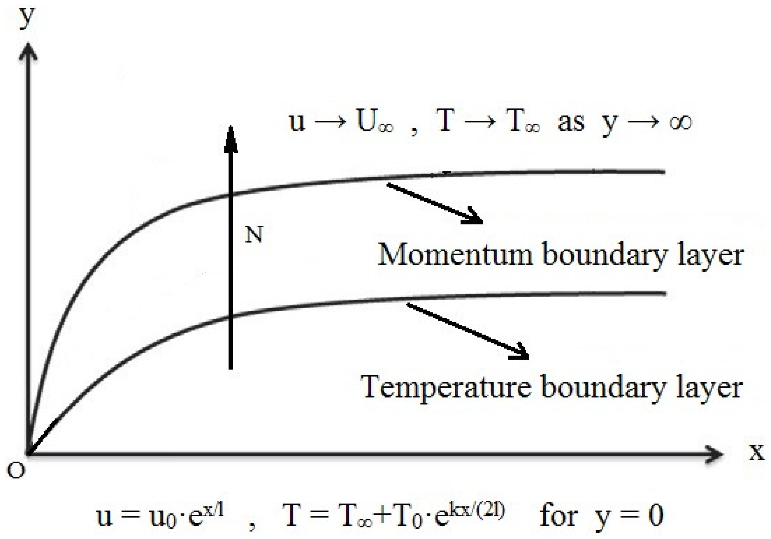
In this section, the two-dimensional flow of an incompressible viscous fluid passes a continuous stretching surface in the half-plane, , taking into account the thermal effect. Additionally, the occurrence of the flow without suction/blowing and without partial slip is explored.
The schematic of the physical model is presented in Figure 1.
For the constant pressure at the boundary layer, the continuity, momentum and temperature equations governing the fluid flow are given by [7]:
The physical initial/boundary conditions can be written in the following form [7]:
3. The Modified Optimal Homotopy Asymptotic Method (OHAM)
The steps of the modified OHAM technique [36] are presented in detail below:
- (i)
- The nonlinear differential equation has the following general form:under the boundary/initial conditionswhere is an arbitrary linear operator, is the corresponding nonlinear operator and is an operator describing the boundary conditions.
- (ii)
- The homotopic relation is given by:where is a given continuous function, is the embedding parameter and is an auxiliary convergence–control function depending on the variable and of the convergence–control parameters , , …, , and choosing the unknown function in the following form:and by equating the coefficients of and , respectively, we obtain:
- -
- the zeroth-order deformation problem
- -
- the first-order deformation problem
- (iii)
- could be obtained by solving the linear Equation (12).
- (iv)
- In Equation (13), the expression has the following general form:where n is a positive integer, and and are known elementary functions that depend on and on .The Equation (13) is a non-homogenous differential equation.By means of the general theory of the differential equations, the computation of the function has the following form:orwhere is an arbitrary number.The above expressions of contain linear combinations of the elementary functions , and the parameters , .
- (v)
The parameters , , …, can be optimally identified by means of various methods, such as the Galerkin method, the collocation method, the Kantorowich method, the least square method or the weighted residual method.
Thus, the first-order approximate solution (17) is well-determined.
4. Heat and Mass Transfer Problem
The skin-friction coefficient is for the first solution and for the corresponding dual solution, respectively.
Using the same modified OHAM procedure, the approximate solutions, denoted by of Equations (6) and (7) (for the unknown function ), were obtained.
The expression of the linear operator could be:
where is an unknown parameter at this moment.
From Equation (6), the nonlinear operator corresponding to the unknown function becomes:
There are a number of possibilities to choose from for the known function , including the following:
or
or
or
and so on.
4.1. The Zeroth-Order Deformation Problem
4.2. The First-Order Deformation Problem
Taking into account the function (22), the nonlinear operator from Equation (19) is:
where the unknown convergence-control parameters , , , , , , , , , will be optimally identified and they depend on , , , K (, for the first solution and , for the corresponding dual solution, respectively [50]) and the physical parameters , k, respectively.
4.3. The First-Order Analytical Approximate Solution
5. Results and Discussion
The accuracy of the obtained results is shown by comparison of the above obtained approximate solutions with the corresponding numerical integration results, computed by means of the shooting method combined with the fourth-order Runge-Kutta method using Wolfram Mathematica 9.0 software. The goal of this section is to compute the convergence-control parameters , , , , and , which appear in Equation (28), by the least square method for different values of the known parameters k and .
For fixed value of the parameter k and different values of the Prandtl number , four approximate solutions for temperature obtained from Equation (28), are presented below:
- (a1)
- the parameter , the Prandtl number .
The first-order approximate solution is:
and the corresponding dual approximate solution becomes:
Other cases (a–a) for different values of the physical parameters k and are treated in Appendix A.
Table 1 and Table 2 provides a comparison between the OHAM approximate solutions (temperature) given by Equations (29), (A1) and (A3) for the first solution, and the corresponding dual approximate solutions (temperature) given by Equations (30), (A2) and (A4), and numerical results for for different values of the Prandtl number .
In Table 3 and Table 4, respectively, the effect of the mass transfer coefficient obtained from Equations (29), (A1), (A3) and (A5) for both approximate solutions and corresponding numerical values are presented.
In the case of the approximate solution given by Equation (28), the residual from Equation (6) becomes:
The numerical values of the integral of the square residual given by Equation (31) are shown in Table 5.
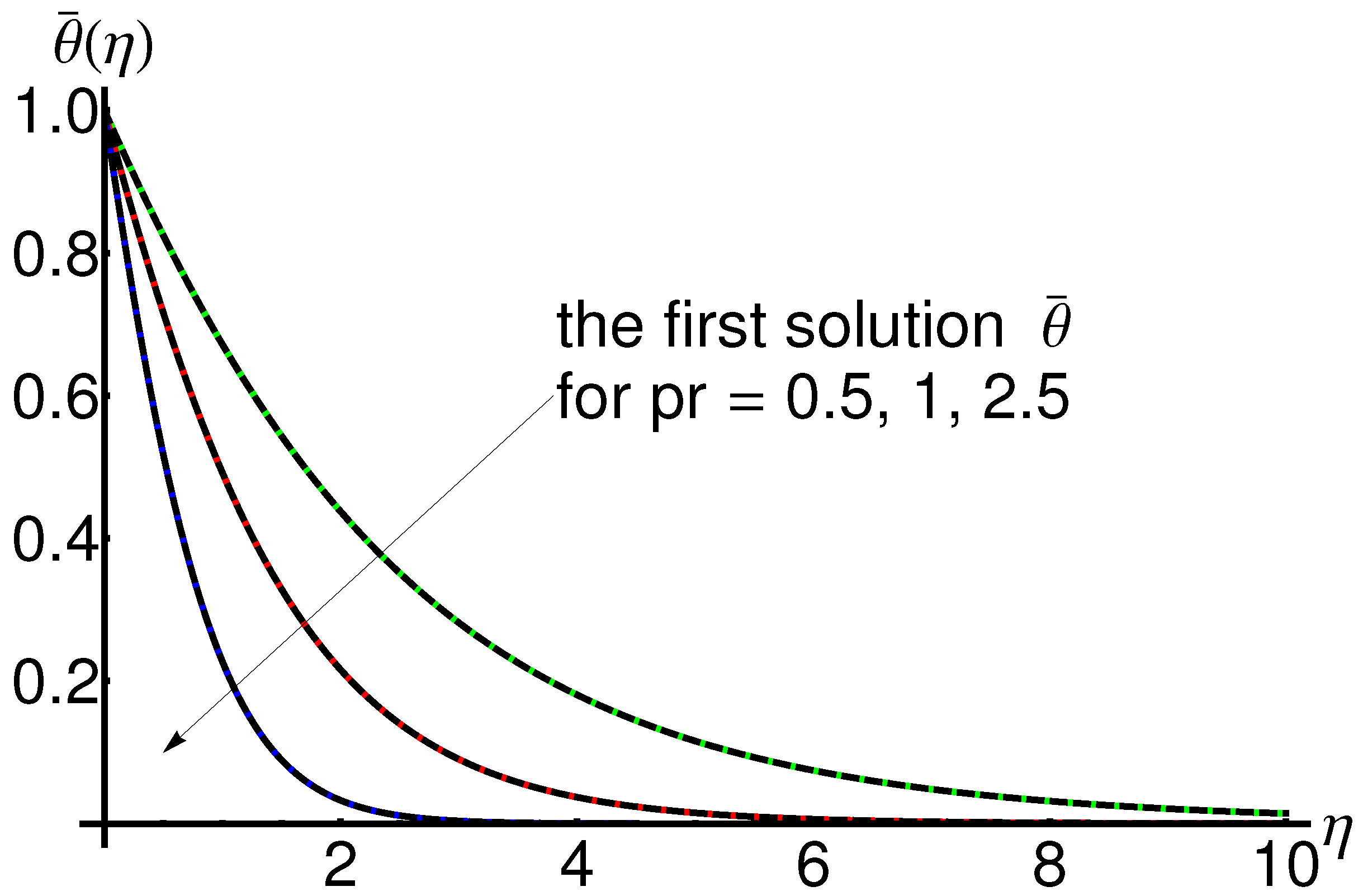
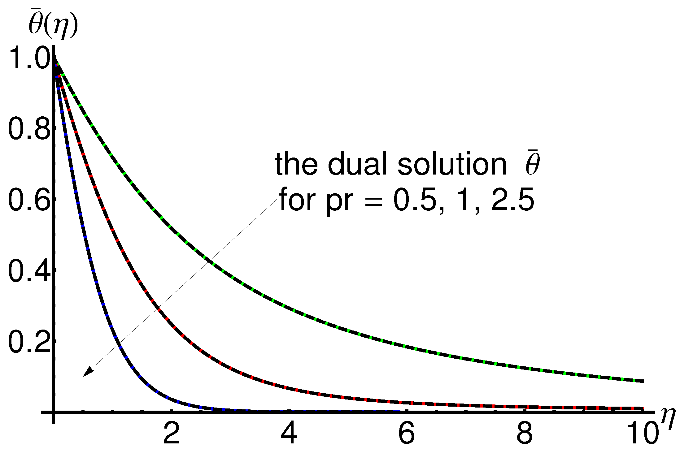
5.1. Influence of the Prandtl Number
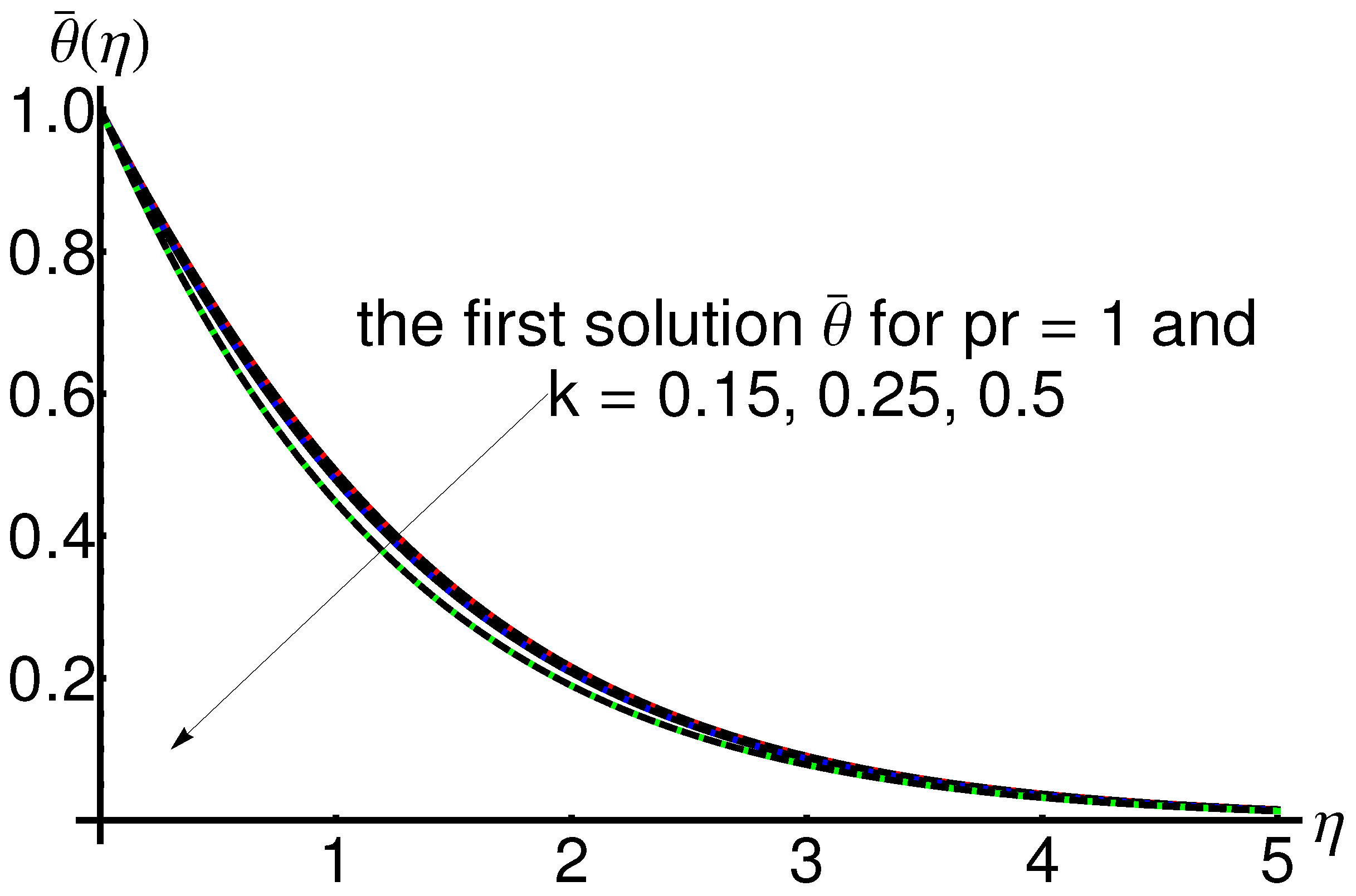
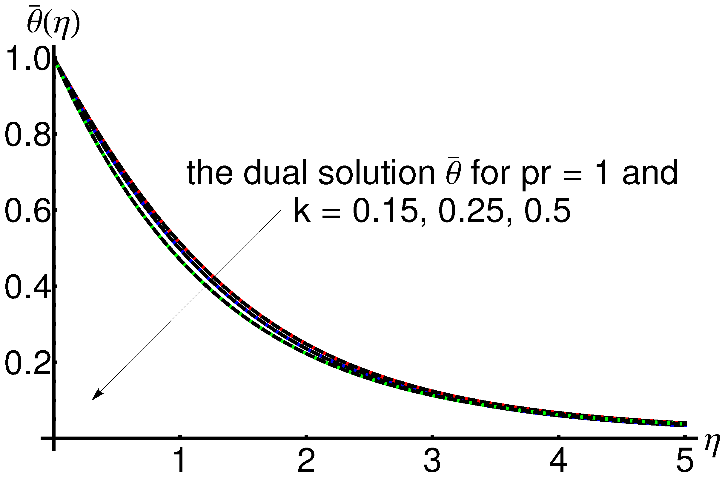
5.2. Influence of the Temperature Distribution Parameter k
Additionally, Figure 6 and Figure 7 show that the variation of the temperature decreases with the increase in the parameter k for some fixed values of the Prandtl number .
From all the Table 1, Table 2, Table 3, Table 4 and Table 5 and Figure 2, Figure 3, Figure 4, Figure 5, Figure 6 and Figure 7 we can summarize that the OHAM solutions are effective and very accurate.
The advantages of the modified OHAM technique by comparison of the OHAM-solutions with the corresponding iterative solutions obtained by means of the iterative method developed in [51] are presented below.
By integration of the system (32) over the interval , the following expressions are obtained:
The iterative algorithm is written as:
Using five iterations, with the initial conditions , , , , (presented in the Table 3) and the physical constants , , taking into account of the algorithm (33), the iterative solutions become:
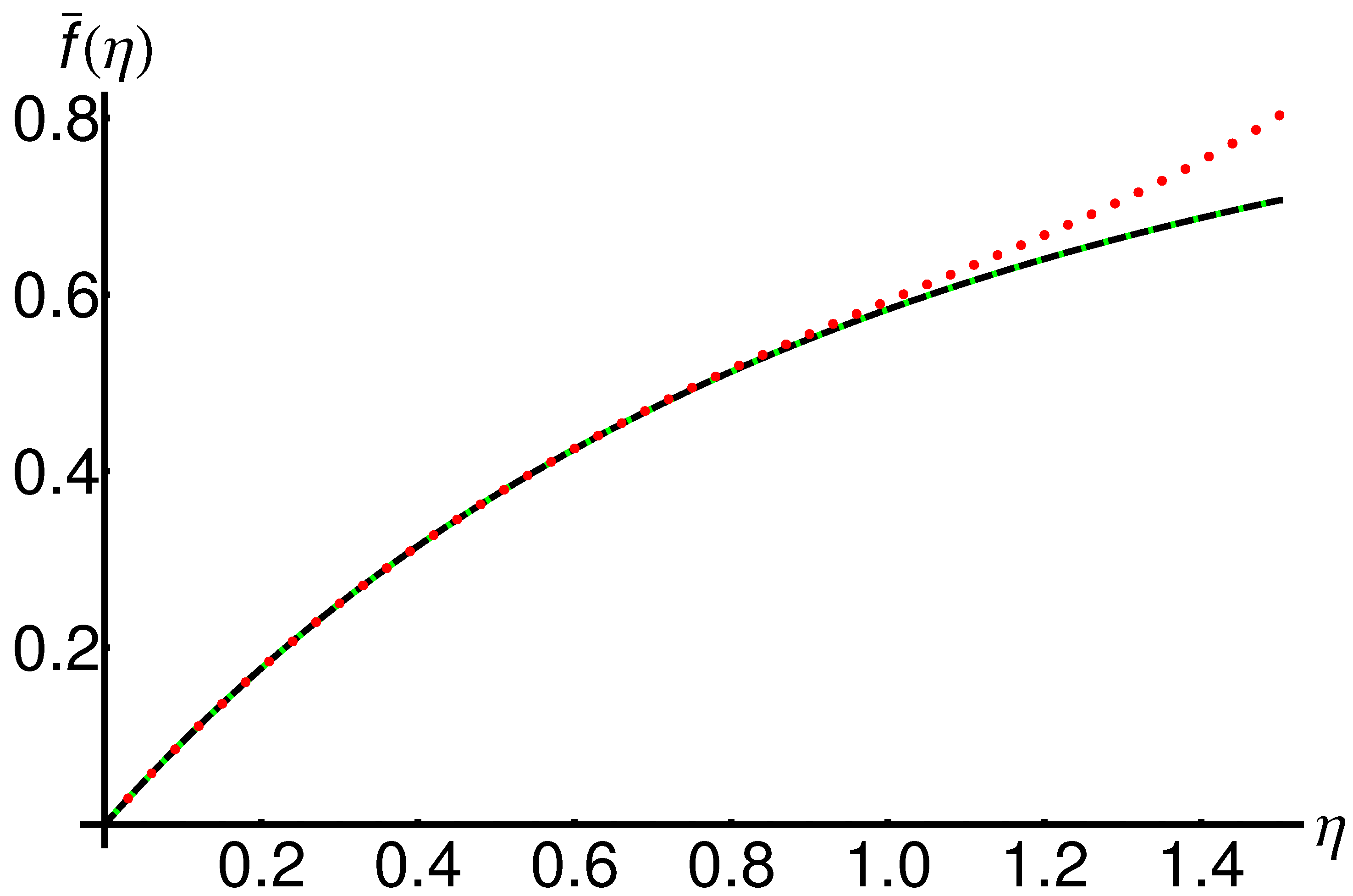
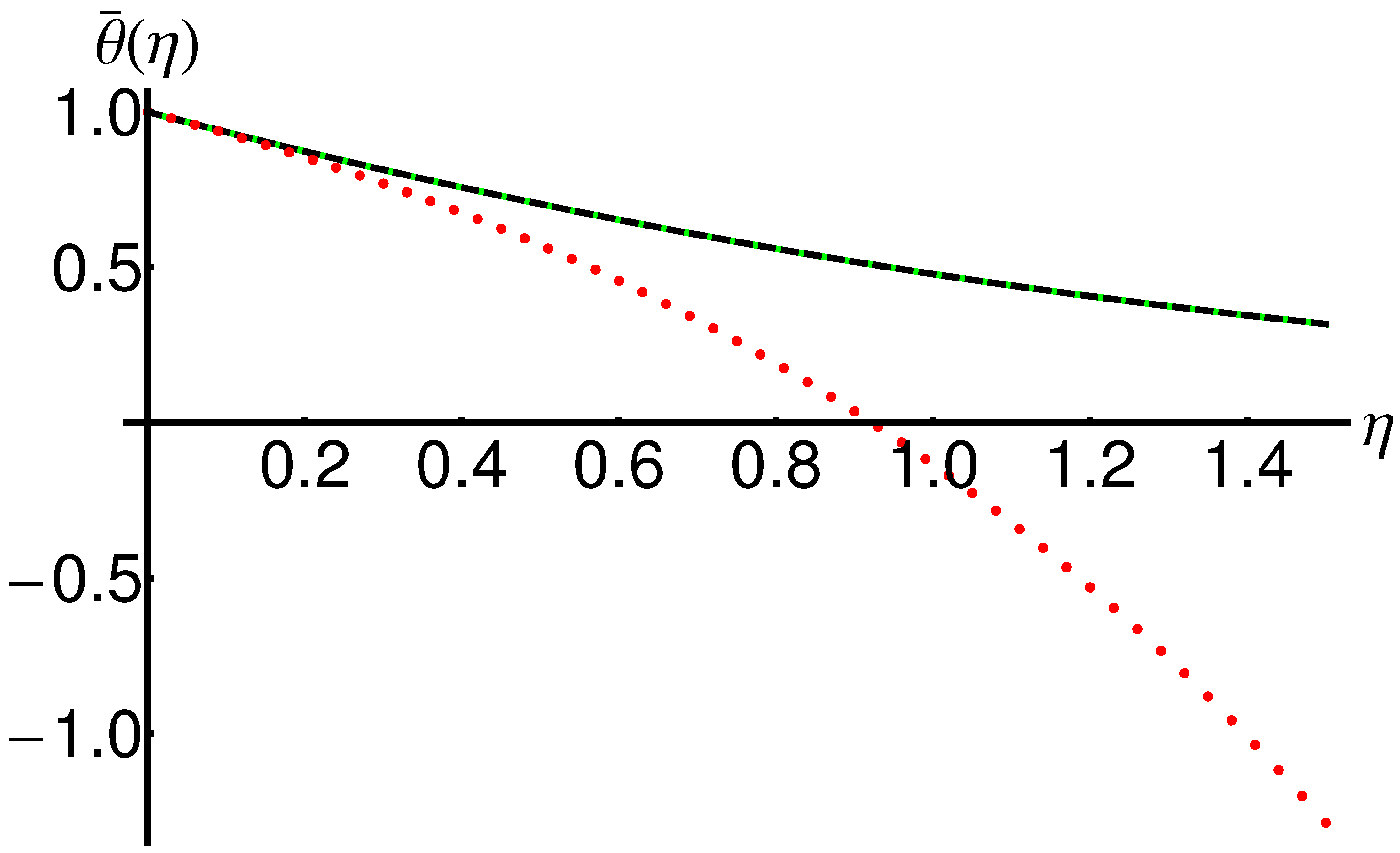
A comparison between the OHAM solutions , and the corresponding iterative solutions , given in Equation (35) is highlighted graphically in Figure 8 and Figure 9 and tabularly in Table 6, respectively.
The precision and efficiency of the OHAM method (using just one iteration) against to the iterative method described in [51] (using five iterations) arising from the presented comparison.
Case Study
In the following we apply our analytical results in the case of the hydraulic oil with a large application at the hydraulic drive systems as turbines, pumps, naval propellers.
We consider the fluid flow scenario from a hydraulic installation with the following values of the characteristic quantities: the reference velocity [m/s], the reference temperature , the kinematical viscosity [m/s] and the environmental temperature , respectively.
6. Conclusions
The steady boundary layer flow and heat transfer over a stretching sheet were analyzed by using a nonlinear differential equation. The variation of the temperature decreases with the increase in the Prandtl number for some fixed values of the parameter k. As a result, we can observe a decrease in the fluid temperature. This shows that more heat is released from the sheet and the Prandtl number decreases in the boundary layer thickness. Therefore, the heat transfer rate increases.
The processes with strongly nonlinear behaviors appear in different technological applications. Thus, an approximate analytical solution is a more realistic option.
The OHAM treatment related to the heat and mass transfer problem without partial slip in the flow of a viscous fluid over an exponentially stretching sheet without suction/blowing is considered and provides an accurate solution for the nonlinear differential equation with initial and boundary conditions.
In this paper, the thermal effects of the Prandtl number and the temperature distribution parameter are analytically analyzed. The variations of the dimensionless surface temperature and heat transfer characteristics with the governing parameters are graphed and tabulated. In particular, the analytically obtained results are applied from the hydraulic system.
The advantage of the method applied in this work is the efficiency by only one iteration. Other advantages, including accuracy, flexibility, validity and convergence, of the approximate solutions are highlighted by comparing the OHAM solutions with the corresponding iterative solutions.
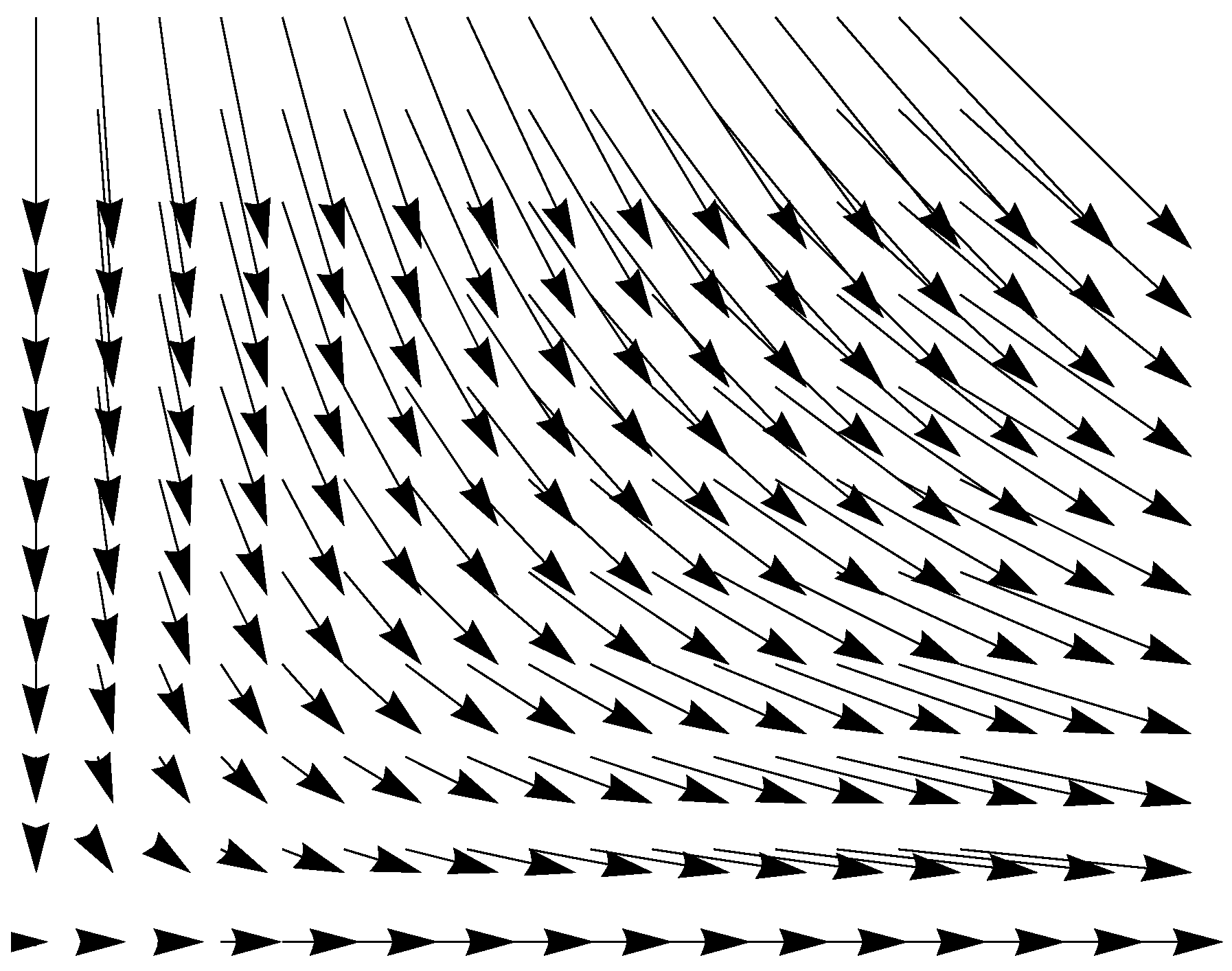
Some characteristics of the heat and mass transfer, such as the vector field and the temperature profile T are graphically depicted in a case study of the hydraulic oil using the obtained approximate solutions via OHAM.
This study is useful for many engineering applications of heat and mass transfer problems such as strand casting processes, polymeric liquids, the extraction of metals and polymers, glass-fiber production, and physiological fluid dynamics.
Author Contributions
Conceptualization, N.P.; data curation, R.-D.E. and N.P.; formal analysis, N.P.; investigation, R.-D.E. and R.B.; methodology, R.-D.E. and R.B.; software, R.-D.E.; supervision, N.P.; validation, R.-D.E. and N.P.; visualization, R.-D.E. and N.P.; writing—original draft, R.-D.E., R.B. and N.P. All authors have read and agreed to the published version of the manuscript.
Funding
This research received no external funding.
Institutional Review Board Statement
Not applicable.
Informed Consent Statement
Not applicable.
Data Availability Statement
Not applicable.
Conflicts of Interest
The authors declare no conflict of interest.
Nomenclature/Notation
| Symbols | Names |
| u, | Velocity components (m/s) |
| x, | Cartesian coordinates (m) |
| Kinematical viscosity (m/s) | |
| Viscosity | |
| Fluid density | |
| Velocity of uniform flow | |
| , | Reference velocity and reference temperature |
| N | Velocity slip factor |
| l | Characteristic length |
| Prandtl number | |
| k | Parameter of temperature distribution |
| Environment temperature (K) | |
| Independent dimensionless variable | |
| Stream function | |
| Temperature | |
| OHAM solution | approximate analytical solution by means of the modified Optimal Homotopy Asymptotic Method |
Appendix A
In this section there are presented in details the first-order approximate solution given by Equation (28) and the corresponding dual solution for different values of the physical parameters.
- (a2)
- the parameter , the Prandtl number .
- (a3)
- the parameter , the Prandtl number .
- (a4)
- the parameter , the Prandtl number .
The influence of the temperature distribution parameter k on the heat transfer is presented below. In this way, we provide the approximate analytical solutions for the case of and different values for k.
- (a5)
- In this case, we consider and .
- (a6)
- In the second case, if and , then:
- (a7)
- In the third case, if and :
In this way, we can construct other accurate approximate solutions.
References
- Sparrow, E.M.; Cess, R.D. Temperature dependent heat sources or sinks in a stagnation point flow. Appl. Sci. Res. 1961, A10, 185. [Google Scholar] [CrossRef]
- Topper, L. Heat transfer in cylinders with heat generation. Am. Inst. Chem. Fagug. J. 1955, 463, 463–466. [Google Scholar] [CrossRef]
- Khashi, N.S.; Waini, I.; Kasim, A.R.M.; Zainal, N.A.; Ishak, A.; Pop, I. Magnetohydrodynamic and viscous dissipation effects on radiative heat transfer of non-Newtonian fluid flow past a nonlinearly shrinking sheet: Reiner–Philippoff model. Alex. Eng. J. 2022, 61, 7605–7617. [Google Scholar] [CrossRef]
- Vajravelu, K.; Hadjinicolaou, A. Heat transfer in a viscous fluid over a stretching sheet with viscous dissipation and internal heat generation. Int. Comm. Heat Mass Transf. 1993, 20, 417–430. [Google Scholar] [CrossRef]
- Xu, H. Mixed convective flow of a hybrid nanofluid between two parallel inclined plates under wall-slip condition. Appl. Math. Mech. -Engl. Ed. 2022, 43, 113–126. [Google Scholar] [CrossRef]
- Hayat, T.; Muhammad, K.; Alsaedi, A. Melting effect and Cattaneo-Christov heat flux in fourth-grade material flow through a Darcy-Forchheimer porous medium. Appl. Math. Mech. -Engl. Ed. 2021, 42, 1787–1798. [Google Scholar] [CrossRef]
- Bararnia, H.; Gorji, M.; Domairry, G. An Analytical Study of Boundary Layer Flows on a Continuous Stretching Surface. Acta Appl. Math. 2009, 106, 125–133. [Google Scholar] [CrossRef]
- Khan, N.S.; Islam, S.; Gul, T.; Khan, I.; Khan, W.; Ali, L. Thin film flow of a second grade fluid in a porous medium past a stretching sheet with heat transfer. Alex. Eng. J. 2018, 57, 1019–1031. [Google Scholar] [CrossRef]
- Khan, N.S.; Gul, T.; Islam, S.; Khan, I.; Alqahtani, A.M.; Alshomrani, A.S. Magnetohydrodynamic Nanoliquid Thin Film Sprayed on a Stretching Cylinder with Heat Transfer. Appl. Sci. 2017, 7, 271. [Google Scholar] [CrossRef]
- Khan, N.S.; Gul, T.; Kumam, P.; Shah, Z.; Islam, S.; Khan, W.; Zuhra, S.; Arif, S. Influence of Inclined Magnetic Field on Carreau Nanoliquid Thin Film Flow and Heat Transfer with Graphene Nanoparticles. Energies 2019, 12, 1459. [Google Scholar] [CrossRef]
- Khan, N.S.; Zuhra, S. Boundary layer flow and heat transfer in a thin-film second-grade nanoliquid embedded with graphene nanoparticles. Adv. Mech. Eng. 2019, 11, 1–11. [Google Scholar] [CrossRef]
- Zuhra, S.; Khan, N.S.; Khan, M.A.; Islam, S.; Khan, W.; Bonyah, E. Flow and heat transfer in water based liquid film fluids dispensed with graphene nanoparticles. Results Phys. 2018, 8, 1143–1157. [Google Scholar] [CrossRef]
- Bilal, A.M.; Alsaedi, A.; Hayat, T.; Shehzad, S.A. Convective Heat and Mass Transfer in Three-Dimensional Mixed Convection Flow of Viscoelastic Fluid in Presence of Chemical Reaction and Heat Source/Sink. Comp. Math. Math. Phys. 2017, 57, 1066–1079. [Google Scholar] [CrossRef]
- Shehzad, S.A.; Hayat, T.; Alsaedi, A. Flow of a thixotropic fluid over an exponentially stretching sheet with heat transfer. J. Appl. Mech. Tech. Phy. 2016, 57, 672–680. [Google Scholar] [CrossRef]
- Alizadeh, Y.; Mosaddeghi, M.R.; Khazayinejad, M. Semi-analytical assessment of heat transfer rate for MHD transient flow in a semi-porous channel considering heat source and slip effect. Waves Random Complex Media 2021, 1–23. [Google Scholar] [CrossRef]
- Yan, H.; Sedighi, M.; Xie, H. Thermally induced diffusion of chemicals under steady-state heat transfer in saturated porous media. Int. J. Heat Mass Tran. 2020, 153, 119664. [Google Scholar] [CrossRef]
- Nadeem, J.; Marwat, D.N.K.; Khan, T.S. Heat transfer in viscous flow over a heated cylinder of nonuniform radius. Ain Shams Eng. J. 2021, 12, 4189–4199. [Google Scholar]
- Abbasi, A.; Khan, S.U.; Farooq, W.; Mughal, F.M.; Khan, M.I.; Prasannakumara, B.C.; El-Wakad, M.T.; Guedri, K.; Galal, A.M. Peristaltic flow of chemically reactive Ellis fluid through an asymmetric channel: Heat and mass transfer analysis. Ain Shams Eng. J. 2023, 14, 101832. [Google Scholar] [CrossRef]
- Xie, W.A.; Xi, G.N. Flow instability and heat transfer enhancement of unsteady convection in a step channel. Alex. Eng. J. 2022, 61, 7377–7391. [Google Scholar] [CrossRef]
- Abdelaziz, A.H.; El-Maghlany, W.M.; El-Din, A.A.; Alnakeeb, M.A. Mixed convection heat transfer utilizing Nanofluids, ionic Nanofluids, and hybrid nanofluids in a horizontal tube. Alex. Eng. J. 2022, 61, 9495–9508. [Google Scholar] [CrossRef]
- Muhammad, K.; Hayat, T.; Alsaedi, A. OHAM analysis of fourth-grade nanomaterial in the presence of stagnation point and convective heat-mass conditions. Waves Random Complex Media 2021, 1–17. [Google Scholar] [CrossRef]
- Mabood, F.; Lorenzini, G.; Pochai, N.; Ibrahim, S.M. Effects of prescribed heat flux and transpiration on MHD axisymmetric flow impinging on stretching cylinder. Contin. Mech. Therm. 2016, 28, 1925–1932. [Google Scholar] [CrossRef]
- Eid, M.R.; Nafe, M.A. Thermal conductivity variation and heat generation effects on magneto-hybrid nanofluid flow in a porous medium with slip condition. Waves Random Complex Media 2020. [Google Scholar] [CrossRef]
- Boumaiza, N.; Kezzar, M.; Eid, M.R.; Tabet, I. On numerical and analytical solutions for mixed convection Falkner-Skan flow of nanofluids with variable thermal conductivity. Waves Random Complex Media 2019. [Google Scholar] [CrossRef]
- Gireesha, B.J.; Keerthi, M.L.; Sowmya, G. Effects of stretching/shrinking on the thermal performance of a fully wetted convective-radiative longitudinal fin of exponential profile. Appl. Math. Mech.-Engl. Ed. 2022, 43, 389–402. [Google Scholar] [CrossRef]
- Waini, I.; Ishak, A.; Pop, I. Magnetohydrodynamic flow past a shrinking vertical sheet in a dusty hybrid nanofluid with thermal radiation. Appl. Math. Mech.-Engl. Ed. 2022, 43, 127–140. [Google Scholar] [CrossRef]
- Tang, Q.; Huang, Y. Parallel finite element computation of incompressible magnetohydrodynamics based on three iterations. Appl. Math. Mech. -Engl. Ed. 2022, 43, 141–154. [Google Scholar] [CrossRef]
- Cveticanin, L. Exact Closed-Form Solution for the Oscillator with a New Type of Mixed Nonlinear Restitution Force. Mathematics 2023, 11, 596. [Google Scholar] [CrossRef]
- Raduca, M.; Hatiegan, C.; Pop, N.; Raduca, E.; Gillich, G.-R. Finite element analysis of heat transfer in transformers from high voltage stations. J. Therm. Anal. Calorim. 2014, 18, 1355–1360. [Google Scholar] [CrossRef]
- Martin, M.J.; Boyd, I.D. Momentum and heat transfer in a laminar boundary layer with slip flow. J. Thermo Heat Trans. 2006, 20, 710–719. [Google Scholar] [CrossRef]
- Anderson, H.I. Slip flow past a stretching surface. Acta Mech. 2002, 158, 121–125. [Google Scholar] [CrossRef]
- Khan, N.S.; Zuhra, S.; Shah, Z.; Bonyah, E.; Khan, W.; Islam, S.; Khan, A. Hall current and thermophoresis effects on magnetohydrodynamic mixed convective heat and mass transfer thin film flow. J. Phys. Commun. 2019, 3, 035009. [Google Scholar] [CrossRef]
- Nayak, M.K.; Mabood, F.; Dogonchi, A.S.; Ramadan, K.M.; Tlili, I.; Khan, W.A. Entropy optimized assisting and opposing non-linear radiative flow of hybrid nanofluid. Waves Random Complex Media 2022, 1–22. [Google Scholar] [CrossRef]
- Cortell, R. Viscous flow and heat transfer over a nonlinearly stretching sheet. Appl. Math. Comput. 2007, 184, 864–873. [Google Scholar] [CrossRef]
- Alam, A.; Marwat, D.N.K. Heat and mass transfer on a stretching/shrinking and porous sheet of variable thickness with suction and injection. Proc. Inst. Mechanical Eng. Part C J. Mech. Eng. 2021, 235, 5297–5308. [Google Scholar] [CrossRef]
- Marinca, V.; Herisanu, N. The Optimal Homotopy Asymptotic Method-Engineering Applications; Springer: Berlin/Heidelberg, Germany, 2015. [Google Scholar]
- Marinca, V.; Ene, R.D.; Marinca, B.; Negrea, R. Different approximations to the solution of upper-convected Maxwell fluid over a porous stretching plate. Abstr. Appl. Anal. 2014, 2014, 139314. [Google Scholar] [CrossRef]
- Ene, R.D.; Marinca, V. Approximate solutions for steady boundary layer MHD viscous flow and radiative heat transfer over an exponentially porous stretching sheet. Appl. Math. Comput. 2015, 269, 389–401. [Google Scholar] [CrossRef]
- Ene, R.D.; Szabo, M.A.; Danoiu, S. Viscous flow and heat transfer over a permeable shrinking sheet with partial slip. Mater Plast. 2015, 52, 408–412. [Google Scholar]
- Marinca, V.; Ene, R.D. Dual approximate solutions of the unsteady viscous flow over a shrinking cylinder with Optimal Homotopy Asymptotic Method. Adv. Math. Phys. 2014, 417643. [Google Scholar] [CrossRef]
- Ene, R.D.; Pop, N. Dual approximate solutions for the chemically reactive solute transfer in a viscous fluid flow. Waves Random Complex Media 2021, 1–23. [Google Scholar] [CrossRef]
- Ullah, H.; Nawaz, R.; Islam, S.; Idrees, M.; Fiza, M. The optimal homotopy asymptotic method with application to modified Kawahara equation. J. Assoc. Arab. Univ. Basic Appl. Sci. 2015, 18, 82–88. [Google Scholar] [CrossRef]
- Almousa, M.; Ismail, A. Optimal Homotopy Asymptotic Method for Solving the Linear Fredholm Integral Equations of the First Kind. Abstr. Appl. Anal. 2013, 2013, 278097. [Google Scholar] [CrossRef]
- Golbabai, A.; Fardi, M.; Sayevandc, K. Application of the optimal homotopy asymptotic method for solving a strongly nonlinear oscillatory system. Math. Comput. Model. 2013, 58, 1837–1843. [Google Scholar] [CrossRef]
- Alomari, A.K.; Anakira, N.R.; Hashim, I. Multiple Solutions of Problems in Fluid Mechanics by Predictor Optimal Homotopy Asymptotic Method. Adv. Mech. Eng. 2014, 6, 372537. [Google Scholar] [CrossRef]
- Marinca, V.; Herisanu, N. Application of Optimal Homotopy Asymptotic Method for solving nonlinear equations arising in heat transfer. Int. Commun. Heat Mass. 2008, 35, 710–715. [Google Scholar] [CrossRef]
- Ullah, H.; Islam, S.; Idrees, M.; Arif, M. Solution of Boundary Layer Problems with Heat Transfer by Optimal Homotopy Asymptotic Method. Abstr. Appl. Anal. 2013, 2013, 324869. [Google Scholar] [CrossRef]
- Waqar, K. Optimal homotopy asymptotic method for heat transfer in hollow sphere with robin boundary conditions. Heat Transf. Asian Res. 2014, 43, 124–133. [Google Scholar]
- Ene, R.D.; Marinca, V.; Negrea, R. Optimal Homotopy Asymptotic Method for viscous boundary layer flow in unbounded domain. In Proceedings of the 16th International Symposium on Symbolic and Nnumeric Algoritms for Scientific Computing (SYNASC 2014), Timisoara, Romania, 22–25 September 2014. [Google Scholar]
- Ene, R.D.; Petrisor, C. Some mathematical approaches on the viscous flow problem on a continuous stretching surface: Nonlinear stability and dual approximate analytic solutions. AIP Conf. Proc. 2020, 2293, 350004. [Google Scholar]
- Daftardar-Gejji, V.; Jafari, H. An iterative method for solving nonlinear functional equations. J. Math. Anal. Appl. 2006, 316, 753–763. [Google Scholar] [CrossRef]
- Giles, R.V. Theory and Problems of the Hydraulics, 2nd ed.; Schaum’s Outline Series; McGraw Hill Book Company: New York, NY, USA, 1977. [Google Scholar]
- Greenshields, C.; Weller, H.G. Notes on Computational Fluid Dynamics: General Principles; CFD Direct Limited: Reading, UK, 2022. [Google Scholar]
Figure 1.
Schematic diagram of the physical model.

Figure 2.
Variation of the temperature given by Equations (29), (A1) and (A3) with the Prandtl number for : OHAM solution (with lines) and numerical solution (dashing lines), respectively.

Figure 3.
Variation of the temperature given by Equations (30), (A2) and (A4) with the Prandtl number for : OHAM solution (with lines) and numerical solution (dashing lines), respectively.

Figure 4.
Variation of the temperature given by Equations (29), (A1) and (A3) with the Prandtl number for : OHAM solution (with lines) and numerical solution (dashing lines), respectively.

Figure 5.
Variation of the temperature given by Equations (30), (A2) and (A4) with the Prandtl number for : OHAM solution (with lines) and numerical solution (dashing lines), respectively.

Figure 6.
Variation of the temperature given by Equations (A1), (A7) and (A9) with the parameter for : OHAM solution (with lines) and numerical solution (dashed lines), respectively.

Figure 7.
Variation of the temperature given by Equations (A2), (A8) and (A10) with the parameter for : OHAM solution (with lines) and numerical solution (dashed lines), respectively.

Figure 8.
Comparison between the approximate analytical solution , of the Equation (5) given by Equation [50], the iterative solution given by Equation (35) and the corresponding numerical solution: numerical solution (with lines), OHAM solution (dashed lines), and iterative solution (dotted curve), respectively.

Figure 9.
Comparison between the approximate analytical solution , of the Equation (6) given by Equation (A1), the corresponding numerical solution and the iterative solution given by Equation (35): numerical solution (with lines), OHAM solution (dashed lines), and iterative solution (dotted curve), respectively.

Figure 10.
The vector field from Equation (4) for hydraulic oil at a temperature of 40 °C, in the case of the first-solution given by Equation [50].

Figure 11.
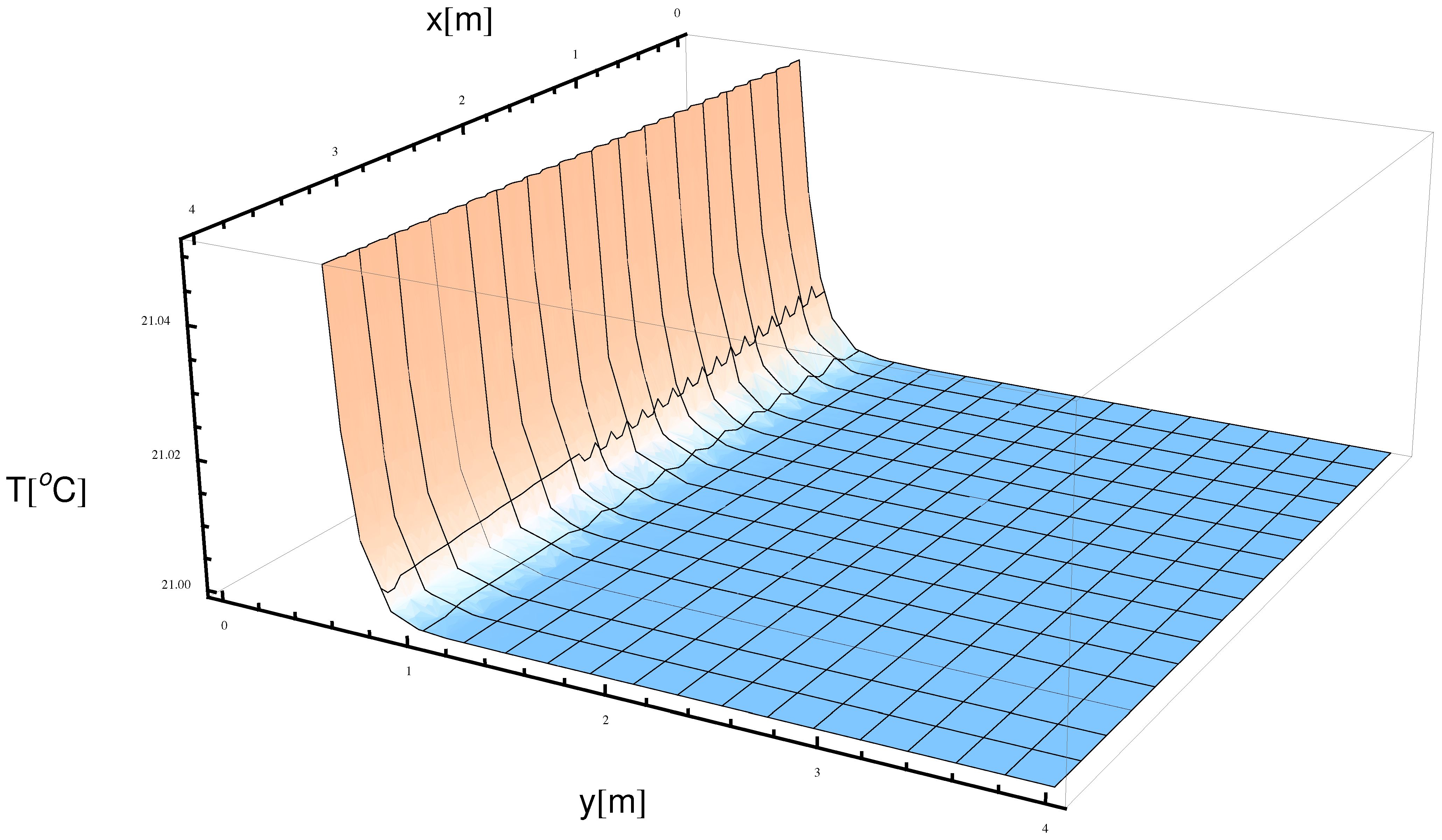
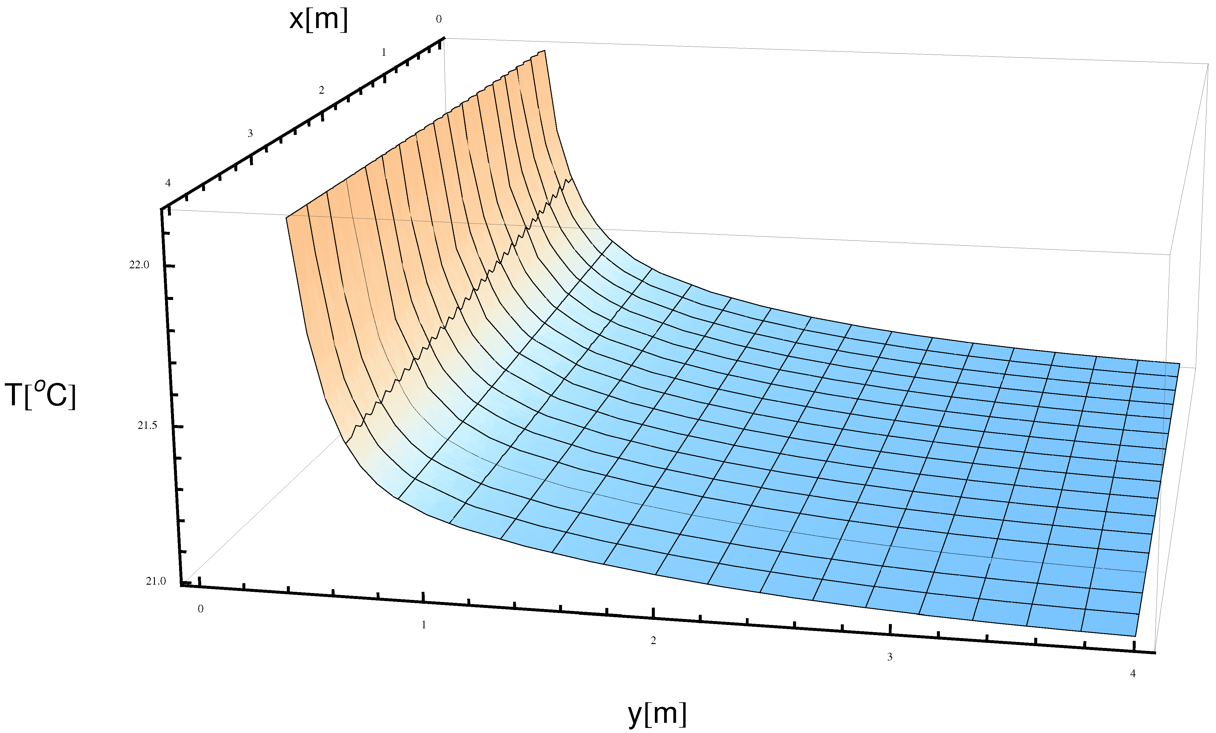
The 3D-profile of the temperature T from Equation (4) for , for hydraulic oil at a temperature of 40 °C, in the case of the first-solution given by Equation (A1).

Figure 12.
The vector field from Equation (4) for hydraulic oil at a temperature of 40 °C, in the case of the corresponding dual solution given by Equation [50].

Figure 13.
The 3D-profile of the temperature T from Equation (4) for , for hydraulic oil at a temperature of 40 °C, in the case of the corresponding dual solution given by Equation (A2).


Table 1.
Comparison between the first-order approximate solutions given by Equations (29), (A1) and (A3) and the corresponding numerical results for and different values of the Prandtl parameter (absolute errors: ).
| 0 | 1 | 1 | 1. |
| 7/10 | 0.7489771062 | 0.6049297342 | 0.3645655020 |
| 7/5 | 0.5542053824 | 0.3451592660 | 0.1026555405 |
| 14/5 | 0.2979176957 | 0.1031937444 | 0.0055540922 |
| 7/2 | 0.2175152070 | 0.0553624933 | 0.0011533541 |
| 21/5 | 0.1586233161 | 0.0295455695 | 0.0002005939 |
| 28/5 | 0.0842151436 | 0.0083554452 | −0.000042451 |
| 7 | 0.0446648315 | 0.0023547811 | −0.000052955 |
| given by Equation (29) | given by Equation (A1) | given by Equation (A3) | |
| 0 | 1 | 1 | 1 |
| 7/10 | 0.7489754987 | 0.6049296367 | 0.3645643475 |
| 7/5 | 0.5542074180 | 0.3451592418 | 0.1026577273 |
| 14/5 | 0.2979183855 | 0.1031938730 | 0.0055556103 |
| 7/2 | 0.2175209607 | 0.0553624331 | 0.0011544802 |
| 21/5 | 0.1586257234 | 0.0295454423 | 0.0001987361 |
| 28/5 | 0.0842093003 | 0.0083555208 | −0.0000415991 |
| 7 | 0.0446671512 | 0.0023548325 | −0.0000527572 |
| for Equation (29) | for Equation (A1) | for Equation (A3) | |
| 0 | 0 | 0 | 0 |
| 7/10 | 1.607455882179920 | 9.742094708720117 | 1.154538486203282 |
| 7/5 | 2.035591219806676 | 2.419851896640068 | 2.186829855102545 |
| 14/5 | 6.897985110887461 | 1.286033818881371 | 1.518143775084551 |
| 7/2 | 5.753703639754804 | 6.013523504849738 | 1.126029875720986 |
| 21/5 | 2.407287287453652 | 1.271883639693272 | 1.857745851002750 |
| 28/5 | 5.843302489164093 | 7.561148052809274 | 8.526737934899268 |
| 7 | 2.319736837258501 | 5.142016535871277 | 1.977883636694968 |
Table 2.
Comparison between the corresponding dual approximate solutions given by Equations (30), (A2) and (A4) and the corresponding numerical results for and different values of the Prandtl parameter (absolute errors: ).
| 0 | 1 | 1 | 1 |
| 7/10 | 0.7858094356 | 0.6190556769 | 0.3688458421 |
| 7/5 | 0.6228249648 | 0.3691930827 | 0.1074930546 |
| 14/5 | 0.4085135781 | 0.1323390363 | 0.0072619140 |
| 7/2 | 0.3388566718 | 0.0822984147 | 0.0019692645 |
| 21/5 | 0.2852286001 | 0.0530118448 | 0.0006029330 |
| 28/5 | 0.2095004124 | 0.0244710236 | 0.0001201557 |
| 7 | 0.1593196243 | 0.0127723199 | 0.0000713911 |
| given by Equation (30) | given by Equation (A2) | given by Equation (A4) | |
| 0 | 1 | 1 | 1 |
| 7/10 | 0.7858136455 | 0.6190546849 | 0.3688476879 |
| 7/5 | 0.6228223796 | 0.3691937408 | 0.1074929959 |
| 14/5 | 0.4085152511 | 0.1323390010 | 0.0072605998 |
| 7/2 | 0.3388541904 | 0.0822992211 | 0.0019705677 |
| 21/5 | 0.2852266049 | 0.0530118072 | 0.0006039728 |
| 28/5 | 0.2095026184 | 0.0244705609 | 0.0001187666 |
| 7 | 0.1593190414 | 0.0127728948 | 0.0000719311 |
| for Equation (30) | for Equation (A2) | for Equation (A4) | |
| 0 | 0 | 0 | 0 |
| 7/10 | 4.209839553404038 | 9.919631346333446 | 1.845765404961952 |
| 7/5 | 2.585204789018469 | 6.580974769021530 | 5.869076206976853 |
| 14/5 | 1.673009802138914 | 3.525957825711856 | 1.314288065634369 |
| 7/2 | 2.481370770357482 | 8.064145169128789 | 1.303131223448148 |
| 21/5 | 1.995245388297650 | 3.768198066078643 | 1.039826044727616 |
| 28/5 | 2.205963331475269 | 4.627662200211435 | 1.389042267445562 |
| 7 | 5.828584578315699 | 5.749493005424017 | 5.400103917853105 |
Table 3.
Comparison between the heat transfer coefficient obtained by means of the OHAM for different values of the Prandtl number and the parameter k, respectively, in the case of the first-order approximate solution.
Table 3.
Comparison between the heat transfer coefficient obtained by means of the OHAM for different values of the Prandtl number and the parameter k, respectively, in the case of the first-order approximate solution.
| Numerical Solution | OHAM Solution | Absolute Errors | ||
|---|---|---|---|---|
| 0.5 | 0.15 | −0.3727417350 | −0.3727417250 | 1.000000127149292 |
| 0.5 | 0.25 | −0.4014940569 | −0.4014939569 | 9.999999639465074 |
| 0.5 | 0.5 | −0.4686586964 | −0.4686585964 | 9.999899136525770 |
| 1 | 0.15 | −0.6171741875 | −0.6171740875 | 9.999999328602627 |
| 1 | 0.25 | −0.6608537627 | −0.6608537527 | 1.000000671158574 |
| 1 | 0.5 | −0.7647932545 | −0.7647931545 | 9.999999373011548 |
| 2.5 | 0.15 | −1.1185512466 | −1.1185511466 | 9.999999783794067 |
| 2.5 | 0.25 | −1.1923711840 | −1.1923710840 | 9.999999694976225 |
| 2.5 | 0.5 | −1.3666535048 | −1.3666534948 | 1.000000171558213 |
Table 4.
Comparison between the heat transfer coefficient obtained by means of the OHAM for different values of the Prandtl number and the parameter k, respectively, in the case of the corresponding dual approximate solution.
Table 4.
Comparison between the heat transfer coefficient obtained by means of the OHAM for different values of the Prandtl number and the parameter k, respectively, in the case of the corresponding dual approximate solution.
| Numerical Solution | OHAM Solution | Absolute Errors | ||
|---|---|---|---|---|
| 0.5 | 0.15 | −0.3238611974 | −0.3238611874 | 1.000000138251522 |
| 0.5 | 0.25 | −0.3473663384 | −0.3473662384 | 9.999999683873995 |
| 0.5 | 0.5 | −0.4014554630 | −0.4014554530 | 1.000000332540551 |
| 1 | 0.15 | −0.5929179987 | −0.5929179887 | 9.999954753148188 |
| 1 | 0.25 | −0.6393617637 | −0.6393617537 | 9.999972516716582 |
| 1 | 0.5 | −0.7402284508 | −0.7402283508 | 9.999999661669534 |
| 2.5 | 0.15 | −1.1110208487 | −1.1110208387 | 1.000000215967134 |
| 2.5 | 0.25 | −1.1848129415 | −1.1848129315 | 1.000000104944831 |
| 2.5 | 0.5 | −1.3591246415 | −1.3591246315 | 1.000000637851883 |
Table 5.
Integral of the square residual given by Equation (31) respectively, for different values of the parameters k and .
Table 5.
Integral of the square residual given by Equation (31) respectively, for different values of the parameters k and .
| The First Solution | The Corresponding Dual Solution | ||
|---|---|---|---|
| 0.15 | 0.5 | 6.575432601542083 | 2.908978433213571 |
| 0.25 | 0.5 | 2.692683749426807 | 6.130825386312505 |
| 0.5 | 0.5 | 2.877470397657074 | 2.329753093802392 |
| 0.15 | 1 | 4.686687280794850 | 4.935777384019864 |
| 0.25 | 1 | 2.769513856968707 | 3.168740967468855 |
| 0.5 | 1 | 1.390428703762422 | 9.337205151229265 |
| 0.15 | 2.5 | 2.424695938193004 | 1.109703562037575 |
| 0.25 | 2.5 | 2.547691207587611 | 8.786794816590718 |
| 0.5 | 2.5 | 3.953512700816478 | 5.589488626508835 |
Table 6.
Comparison between the approximate analytical solution given by Equation [50], the iterative solution given by Equation (35) and the corresponding numerical solution.
| [50] | |||
|---|---|---|---|
| 0 | 0 | 0 | 0 |
| 1/10 | 0.0939089690 | 0.0939087919 | 0.0939089962 |
| 1/5 | 0.1767959477 | 0.1767950192 | 0.1767969422 |
| 3/10 | 0.2501798542 | 0.2501779276 | 0.2501903246 |
| 2/5 | 0.3153313350 | 0.3153286203 | 0.3153863643 |
| 1/2 | 0.3733200865 | 0.3733170634 | 0.3735172090 |
| 3/5 | 0.4250519374 | 0.4250491302 | 0.4256065973 |
| 7/10 | 0.4712981406 | 0.4712959627 | 0.4726209608 |
| 4/5 | 0.5127187008 | 0.5127173844 | 0.5155172621 |
| 9/10 | 0.5498810935 | 0.5498806830 | 0.5552901957 |
| 1 | 0.5832753856 | 0.5832757722 | 0.5930217087 |
Disclaimer/Publisher’s Note: The statements, opinions and data contained in all publications are solely those of the individual author(s) and contributor(s) and not of MDPI and/or the editor(s). MDPI and/or the editor(s) disclaim responsibility for any injury to people or property resulting from any ideas, methods, instructions or products referred to in the content. |
© 2023 by the authors. Licensee MDPI, Basel, Switzerland. This article is an open access article distributed under the terms and conditions of the Creative Commons Attribution (CC BY) license (https://creativecommons.org/licenses/by/4.0/).
Share and Cite
MDPI and ACS Style
Ene, R.-D.; Pop, N.; Badarau, R. Heat and Mass Transfer Analysis for the Viscous Fluid Flow: Dual Approximate Solutions. Mathematics 2023, 11, 1648. https://doi.org/10.3390/math11071648
AMA Style
Ene R-D, Pop N, Badarau R. Heat and Mass Transfer Analysis for the Viscous Fluid Flow: Dual Approximate Solutions. Mathematics. 2023; 11(7):1648. https://doi.org/10.3390/math11071648
Chicago/Turabian StyleEne, Remus-Daniel, Nicolina Pop, and Rodica Badarau. 2023. "Heat and Mass Transfer Analysis for the Viscous Fluid Flow: Dual Approximate Solutions" Mathematics 11, no. 7: 1648. https://doi.org/10.3390/math11071648
Note that from the first issue of 2016, this journal uses article numbers instead of page numbers. See further details here.