
Random Forest and Whale Optimization Algorithm to Predict the Invalidation Risk of Backfilling Pipeline


School of Resources and Safety Engineering, Central South University, Changsha 410083, China
*
Author to whom correspondence should be addressed.
Mathematics 2023, 11(7), 1636; https://doi.org/10.3390/math11071636
Submission received: 13 February 2023
/
Revised: 19 March 2023
/
Accepted: 26 March 2023
/
Published: 28 March 2023
Abstract
:The problem of backfilling pipeline invalidation has become a bottleneck restricting the application and development of backfilling technology. This study applied the whale optimization algorithm and random forest (WOA–RF) to predict the invalidation risk of backfilling pipelines based on 59 datasets from actual mines. Eight influencing factors of backfilling pipeline invalidation risk were chosen as the input parameters of the WOA–RF model, and the risk level was selected as the output parameters of the WOA–RF model. Furthermore, random forest, decision tree, artificial neural network, k-nearest neighbor, and support vector machine models were also established according to the collected datasets. The prediction performance of the six classification models was compared. The evaluated results showed that the established WOA–RF hybrid model has the best prediction performance and the highest accuracy (0.917) compared to other models, with the highest kappa value (0.8846) and MCC value (0.8932). In addition, the performed sensitivity analysis showed that the deviation rate is the most important influencing factor, followed by the internal diameter of the pipeline. Eventually, the WOA–RF hybrid model was used to predict the failure risk level of the backfilling pipelines of nine actual mines in Sichuan, China. The field datasets were collected through field investigation, and engineering verification was carried out. The research results show that the WOA–RF hybrid model is reasonable and effective for backfilling pipeline invalidation risk, and it can provide a novel solution for backfilling pipeline invalidation, with good engineering practicability.
1. Introduction
In the actual production process, the safety of pipelines has a great impact on social and economic aspects, especially the invalidation risk of the pipeline. For example, the transmission process of gas pipelines and oil pipelines is prone to leakage, pipeline explosion, and other accidents [1,2,3], and numerous research experts have conducted many studies on this issue. Aljaroudi et al. [4] assessed the risk of offshore crude oil pipeline failures and predicted the failure of offshore crude oil pipelines. Zhou et al. [5] performed a risk assessment along natural gas pipelines, comprehensively considered the risks of various major accidents, and analyzed the superimposed effect. Tabesh et al. [6] identified the risks of horizontal directional drilling (HDD) pipeline installation, and many of the serious and high-impact risks associated with HDD failures were avoided. Pillay et al. [7] conducted a case study of the current high-pressure subsea pipeline, and the primary research objective was to determine the adequacy of existing risk mitigation measures. Yang et al. [8] analyzed the corrosion failure of submarine pipelines, proposed a method to evaluate the condition of submarine pipelines by analyzing the observed abnormal events, and proved the reliability of the model. Lu et al. [9] adopted the method of combining a risk matrix and bow knot to carry out a comprehensive risk assessment of natural gas pipelines and verified the practicability of the model. Zhang et al. [10] used interval-based AHP (IAHP) and the Technique for Order Preference by Similarity to an Ideal Solution methods (TOPSIS) to identify the risks of hydropower projects to illustrate the application of the hybrid model. Shin et al. [11] considered the effect of corrosion on the risk-based safety management of underground pipelines and adopted risk-based pipeline management, which achieved good results. Mazumder et al. [12] used a data-driven machine learning algorithm for failure risk analysis of pipelines, and the application results illustrated its computational efficiency over physics-based methods. Li et al. [13] proposed a dynamic probabilistic approach to develop accident scenarios by finding fatigue failure causes and derived events using a dynamic Bayesian network. Yu et al. [14] proposed a model that systematically integrates a Bayesian network, fuzzy theory, and a hierarchical analysis process to analyze the probability of pipeline failure, which can be used for quantitative analysis of pipeline failure. Jayan et al. [15] utilized the Bayesian method and bow-tie analysis to obtain the failure frequency of all possible causes of failure. However, the above pipeline risk prediction research is mainly for gas and oil pipelines, not for backfilling pipelines in mining engineering.
In the field of mining, the backfilling method, as a sustainable mining method, is clean, efficient, and green and can effectively solve the problems of surface subsidence and tailings accumulation [16,17]. In practical applications of backfilling mining, a reasonable backfilling system is key to the success of the backfilling mining method. The backfilling conveying pipeline is the throat of the whole backfilling system and the weakest link of the whole backfilling system. Due to the complex environment of backfilling pipelines and their uncertainty, the flow rate, hydraulic gradient, and other slurry fluid parameters and transportation performance of backfilling pipelines are also more complex, and inevitably, there are various potential risks in the production process. The failure of some components in the system will affect the normal operation of the entire backfilling pipeline system, resulting in the failure of the pipeline system, such as pipeline wear, explosion, slurry leakage blocking, and other backfilling pipeline failure accidents [18,19]. Currently, many mines at home and abroad have experienced backfilling pipeline failure accidents, which have seriously affected the normal economic development of mining enterprises and have also become a bottleneck restricting the application and development of mine backfilling technology [20,21,22]. The problem of backfilling pipeline risk prediction is important, which will affect the safety and stability of the backfilling system, but few domestic and foreign scholars have conducted research on this problem. In this paper, a backfilling pipeline risk level prediction model is developed based on intelligent algorithms, and the model provides a decision basis for the failure risk prediction of mine backfilling pipelines. Therefore, it is of great practical significance for the economic development and safe production of mining enterprises to establish a risk prediction model of backfilling pipeline failure and accurately predict the risk level of backfilling pipeline failure.
In recent years, with the development of artificial intelligence (AI) and other computer fields, machine learning (ML) methods have been widely used in science and engineering [23,24,25,26,27,28,29]. At present, the main prediction models include single and hybrid models. For single prediction models, numerous studies have been conducted by domestic and foreign experts. For example, Qi et al. [23] used the random forest (RF) algorithm to predict the open stope hanging wall stability; Ghalambaz et al. [30] used the grey wolf optimizer (GWO) to optimize the building energy, mainly to provide a good archive of non-dominant optimal solutions; Goudos et al. [31] applied a particle swarm optimization (PSO) algorithm to electromagnetic design problems; Naadimuthu et al. [32] used the adaptive neural fuzzy inference system (ANFIS) to design two fuzzy systems; Zhang et al. [33] established a neural network for slope stability prediction, which can be used as a decision-making basis for slope stability analysis. Moreover, for the hybrid model, some researchers have conducted a lot of research, such as Li et al. [34] used SVM and ANN methods to compare the vulnerability evaluation of an urban buried gas pipeline network, and the results showed that this method was effective in practical applications; Mansour [35] proposed a Bayes classifier (BAYES) using independent component analysis and the naive texture classification algorithm; Otero et al. [36] adopted the ant colony optimization(ACO) algorithm to induce a decision tree (DT) with good results; Zhou et al. [37] used support vector machine (SVM) optimized by the whale optimization algorithm (WOA) to predict tunnel extrusion and made classified prediction for tunnel extrusion; Liu et al. [38] used stochastic forest regression and the whale optimization algorithm (WOA) to evaluate the regional flood resistance. The above methods have achieved some results in engineering, showing the importance of machine learning. However, the following shortcomings still exist in the actual prediction process of the models: (1) For a single model, its model results will be worse than the hybrid model results. (2) Only a few models have been used to predict the failure risk of backfilling pipelines, while other algorithms (such as random forest or the whale optimization algorithm) have not been used, which will lead to differences in the model calculation results.
Therefore, a hybrid model combined with the whale optimization algorithm and random forest (WOA–RF) is established in this paper, and the model is applied to the failure risk classification of backfilling pipelines. First, the failure risk database of the mine backfilling pipeline is established, and eight influencing factors are comprehensively considered as the input parameters. In addition, the performance of WOA–RF is compared with other widely used ML models. Finally, sensitivity analysis is performed to evaluate the contribution of each influencing factor to the model and determine the sensitivity variable.
The outline of this study is as follows: Section 2, “Engineering background and database description”, describes the engineering background of fifty-nine mines and the source of the database. Section 3, “Modeling methodology”, describes the principles and components of the RF and WOA model. Furthermore, Section 4, “Modeling results and discussion”, evaluates and compares all classification models, and the optimized model is applied to sensitivity analysis and engineering validation. The study limitations are introduced in Section 5, and the conclusions are given in Section 6.
2. Engineering Background and Database Description
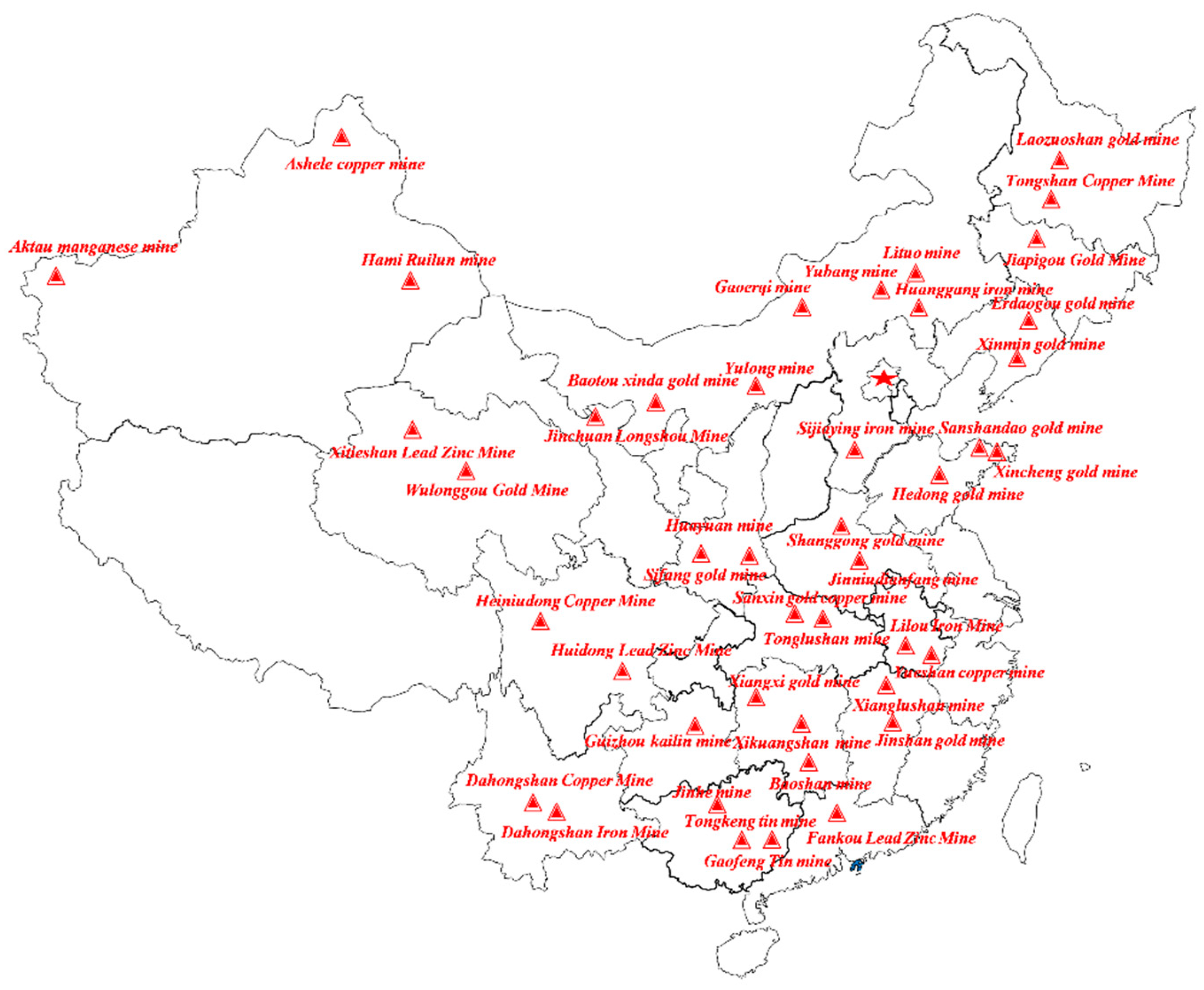
Fifty-nine metal mines in China were investigated, including the Lilou Iron Mine, Jinchuan Longshou Mine, Guizhou Kailin mine, Sanshandao Gold mine, Yunnan Dahongshan Copper Mine, Yunnan Dahongshan Iron Mine, Guanyinsi Lead Mine, etc. These mines are distributed all over the country, with a mining depth of 500~1000 m. In addition, 70% of the mines have an annual output of more than 1 million tons, which are considered large and medium-sized mines; 30% of the mines are small mines. Furthermore, the mining methods are mainly the sectional backfilling method, sectional drilling stage ore drawing followed by the backfilling mining method, and the drift backfilling method. The process flow of the backfilling system is relatively complex. First, the tailings and cement and other cementing materials are vigorously mixed to form a qualified paste backfilling slurry, and then it is pressurized by the backfilling pump and transported to the goaf to be filled through the backfilling pipeline. However, in the whole backfilling process, due to various factors, such as the volume fraction of backfilling slurry, the internal diameter of the pipeline, deviation rate, etc., it is easy to cause backfilling pipeline failure, which will affect normal mining production and easily cause mining safety problems, resulting in loss of personnel and property. The location distribution of 59 metal mines is shown in Figure 1.
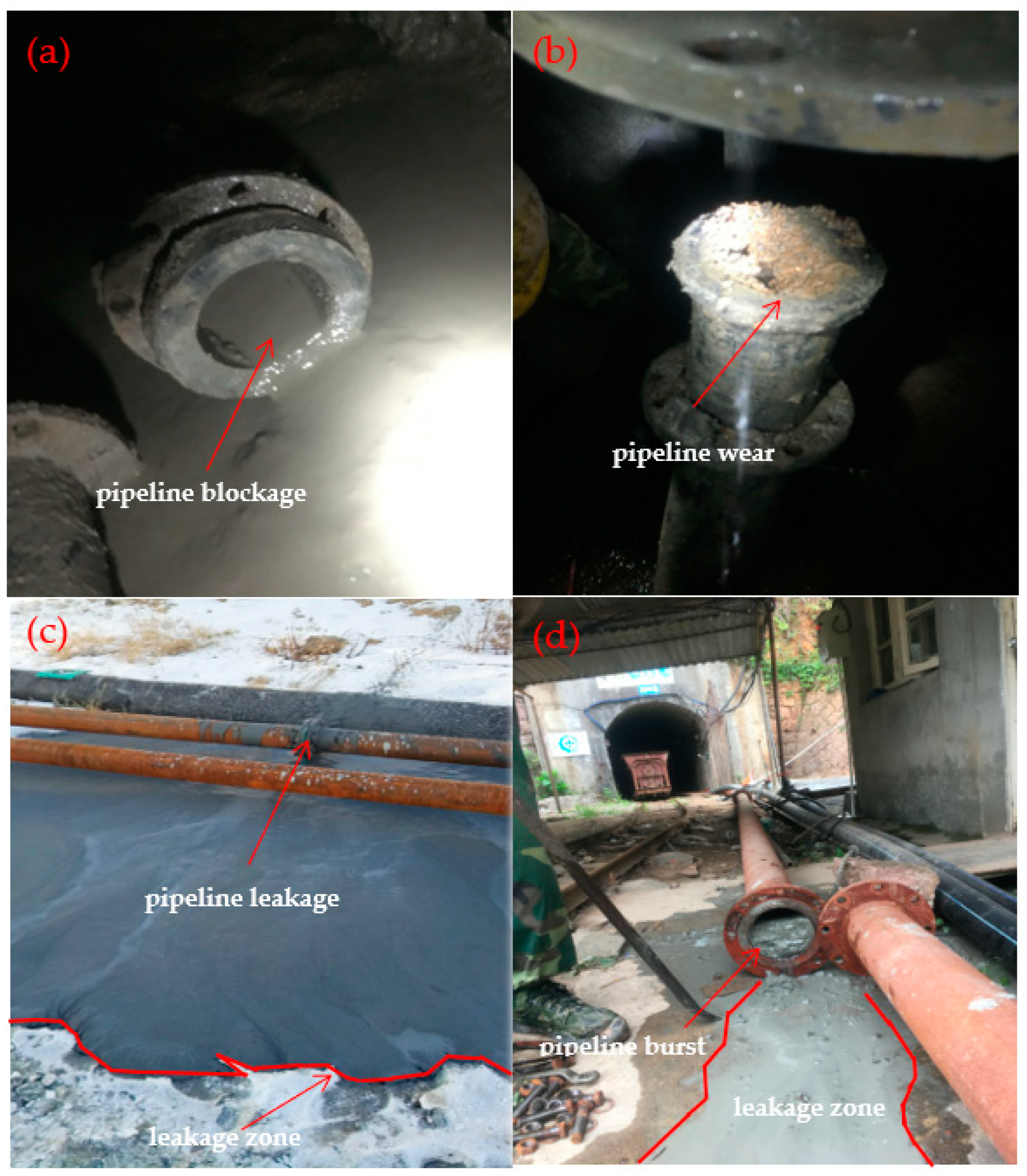
In this study, the data of failure risk classification standards were proposed by many domestic and foreign researchers [39], as shown in Table 1. Considering the characteristics of backfilling slurry and backfilling pipelines, fifty-nine metal mines across China were selected, and eight influencing factors were chosen to establish the backfilling pipeline failure risk dataset. Figure 2 shows that the modes of backfilling pipeline failure include common failure forms: pipeline blockage, pipeline leakage, pipeline burst, and pipeline wear. The risk grade assessment standard was divided into 4 risk levels: extremely dangerous, significant risk, greater risk, and general risk, which were represented by Class 1, Class 2, Class 3, and Class 4, respectively.
Based on the field survey of backfilling pipelines in fifty-nine metal mines in China, the risk data of backfilling pipeline failure in fifty-nine mines are shown in Table 2. Eight influence factors in each specific mine were set as input variables to predict the risk level. The eight influence factors include the volume fraction of backfilling slurry, the density of backfilling slurry, the internal diameter of the pipeline, the deviation rate, the pipeline absolute roughness, the stowing gradient, the ratio of slurry flow rate with critical velocity, and the weighted average particle size. The influencing factors (volume fraction of backfilling slurry, density of the backfilling slurry, weighted average particle size, and ratio of slurry flow rate to critical velocity) can reflect the characteristics of the backfill, and the other four parameters (internal diameter of the pipeline, deviation rate, pipeline absolute roughness, and stowing gradient) reflect the influence of the inherent parameters of the backfilling pipeline on pipeline failure. Each influence factor is as follows:
The volume fraction of backfilling slurry is defined as the volume of the solute of the backfilling slurry as a percentage of the total solution volume.
The density of the backfilling slurry refers to the mass of the backfilling slurry per unit volume.
The deviation rate is the ratio of the depth of the drilling hole to the skews.
The internal diameter of the pipeline is the diameter inside the inner wall of the pipeline.
The absolute roughness of the backfilling pipeline refers to the average height of the protruding part of the wall of the backfilling pipeline.
The stowing gradient is defined as the ratio of the total length of the backfilling pipeline to the height difference of the vertical section of the pipeline in the backfilling pipeline network.
The weighted average particle size is called the particle number average size.
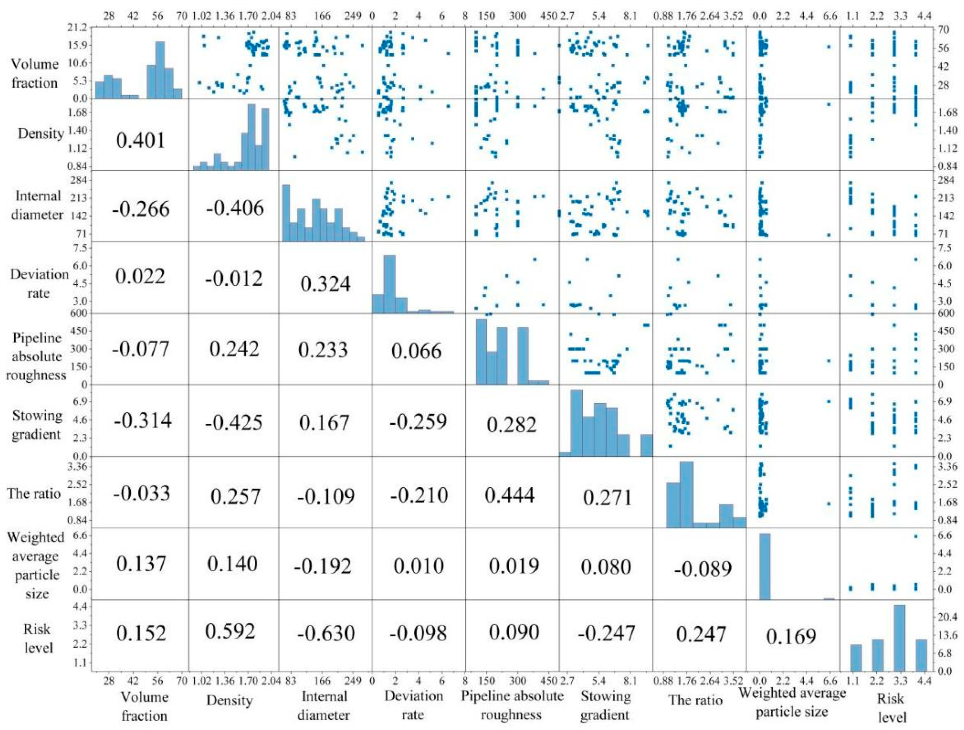
To understand the correlation between input and output variables in the invalidation risk data of a backfilling pipeline, the correlation coefficient matrix of the cumulative distributions and statistical evaluation can be observed in Figure 3. Moreover, the diagonal line of the matrix shows the probability distribution of each influence factor, the lower triangle presents Pearson correlation coefficients, and the upper triangle shows a paired scatterplot of the four classifications of the risk of failure of the backfilling pipeline data along the axis. Figure 3 shows the poor correlation between the influencing factors (R < 0.5) [40,41], and there is no clear distinction between the risk level of extremely dangerous, significant risk, greater risk, and general risk. Therefore, the above correlation coefficient matrix analysis indicates that the relevant parameters can be used for classification modeling of backfilling pipeline failure risk prediction.
3. Modeling Methodology
3.1. Random Forest
RF can effectively solve overfitting and provide an accurate decision tree. It has the advantages of low performance, simple implementation, accurate classification, high accuracy, and fast classification speed [42,43,44,45]. The algorithm training steps are as follows [46,47,48]:
Step 1: The machine selects k training sample sets and k out-of-bag datasets by resampling. The decision tree corresponding to the datasets outside the bag will vote on the samples to obtain the prediction so that the ratio of misclassified samples to total samples is the external bag error. It can be directly generalized using bag error assessment.
Step 2: Randomly select the best features from the feature parameters split attribute nodes that are split for decision tree nodes.
Step 3: Train the decision tree with the training set and the extracted feature subset. K decision trees are obtained from k training sample sets.
Step 4: Linearly integrate the output results of each decision tree to obtain the overall output of the RF algorithm.
3.2. Whale Optimization Algorithm
The WOA was proposed by Mirjalili et al. in 2016 [49]. The algorithm can effectively speed up the optimization rate, and the search strategy of the WOA also has certain advantages in some problems [50]. It includes the following stages: ① encircling the prey; ② spiral bubble; and ③ searching for prey.
(1) Encircling prey
The WOA first determines the best search agent by identifying the location of prey and surrounding it. Other search agents can relocate based on the best search agent. It is mainly expressed by Equations (1) and (2):
where is the best position vector obtained, is the position vector, and A and C represent the coefficient vectors and are calculated using Equations (3) and (4):
where denotes a random vector, a linearly decreases from 2 to 0 with the progress of the iteration, and denotes a random number in [0, 1].
(2) Spiral bubble
Spiral foam hair is used to catch prey and create a spiral equation [51] according to the distance between the whales and prey, as shown in Equation (5):
where is the distance between the whale and its prey, b is a constant that defines the shape of the logarithmic helix, and is a random vector distributed uniformly within [–1, 1].
The WOA selects bubble net predation or constricted enclosure based on the probability p. Therefore, Equation (6) is as follows
where and denotes the probability of predation mechanism probability.
(3) Searching for prey
The WOA requires a global search [52]. Equations (7) and (8) are as follows:
where represents a random position vector.
Therefore, the WOA was used to optimize the ability of RF in predicting the invalidation risk of backfilling pipelines in this paper.
4. Modeling Results and Discussion
4.1. Evaluation Indicators
The performance evaluation indicators of the model were used to analyze and evaluate the quality of the model. The area under the ROC curve is between [0, 1]. The classification accuracy of the model is positively correlated with the area under the ROC curve [53,54]. The MCC is used to measure the classification performance of binary classification in machine learning [55,56]. This indicator combines true positive (TP), true negative (TN), false positive (FP), and false negative (FN). The calculation equation is shown in Equation (9). In addition, the evaluation indicators of the model can be calculated through a confusion matrix [57], as shown in Figure 4.
4.2. Development and Validation of the WOA–RF Model
The main steps of the WOA–RF prediction model analysis of backfilling pipeline failure risk are as follows:
(1) Establish the datasets. Fifty-nine groups of mine backfilling pipeline failure risk data in the database were investigated at many mines in various provinces in China, and the dataset was then randomly divided into a training set (80%) and a testing set (20%) according to the most commonly used splitting ratios of 80% and 20% for model development and model verification, respectively [58,59]. Among them, the number of different risk levels is uniformly distributed in 80% of the training sets and 20% of the testing sets.
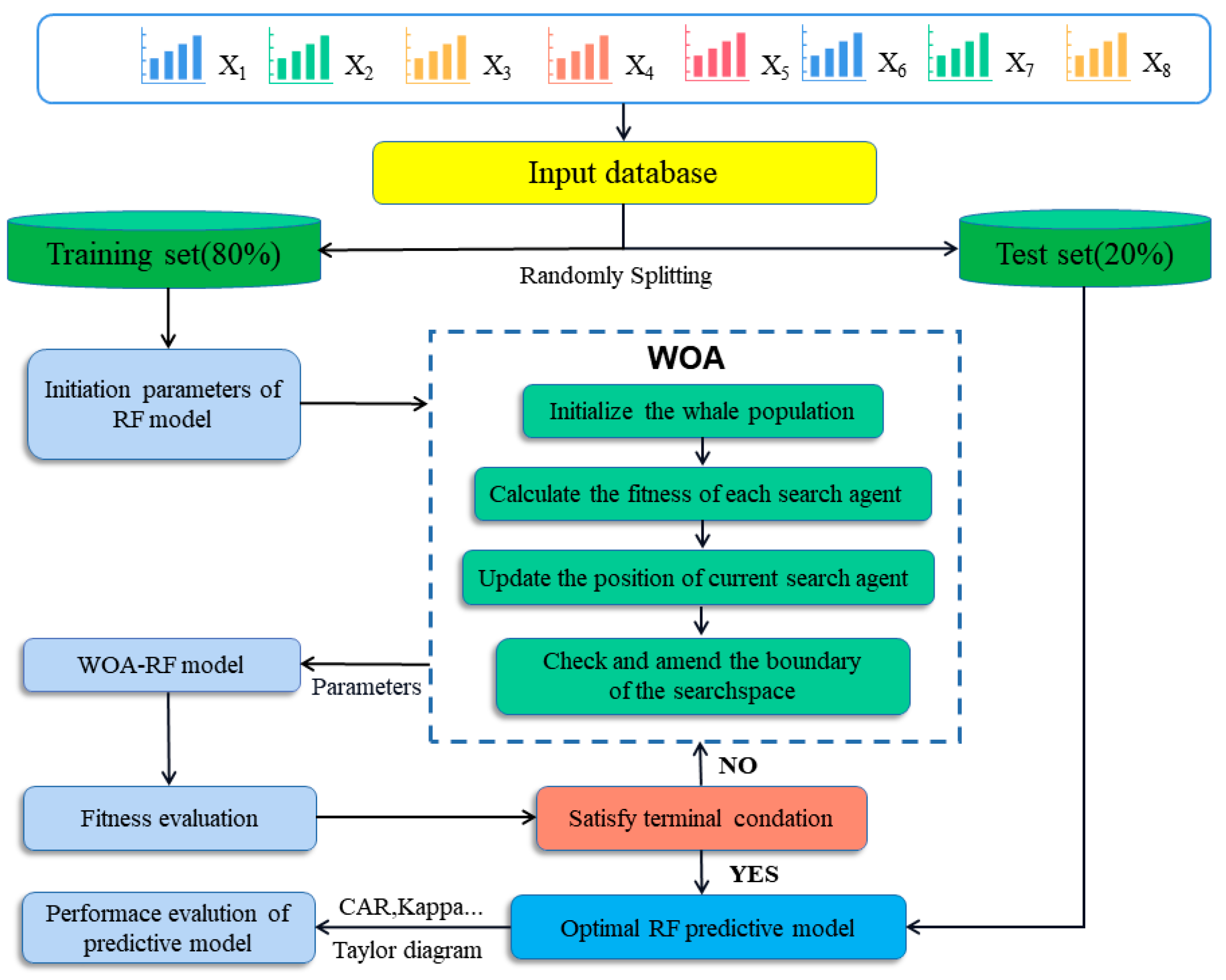
(2) Model development. Initialize the parameters of the RF model. In particular, the RF model hyperparameters of n_estimators (N) and max_features (M) are optimized mainly by the WOA algorithm. In this study, the WOA–RF hybrid model is proposed. Figure 5 shows the optimization analysis process of the WOA–RF model. Each whale position vector is determined by the parameters of the RF model (“n_estimators” and “max_features”). The WOA outputs the final parameters of the RF model after iterating the global optimal position of the search algorithm. That is, the WOA first initializes the whale population, then calculates the fitness of each search agent, and updates the position of the current search agent, checking and correcting the search space boundary. Then, WOA outputs the parameters of the hybrid model to analyze and evaluate the fitness.
(3) Model validation. The relevant parameters of the WOA are constant b and random numbers l and r, where l is distributed in [−1, 1], and r is distributed in [0, 1]. Therefore, the WOA–RF hybrid model should first determine the optimal parameters of the model and then optimize the prediction ability of the RF classifier through the WOA.
In addition, the objective function is defined as Equation (10). Equations (10) and (11) are as follows:
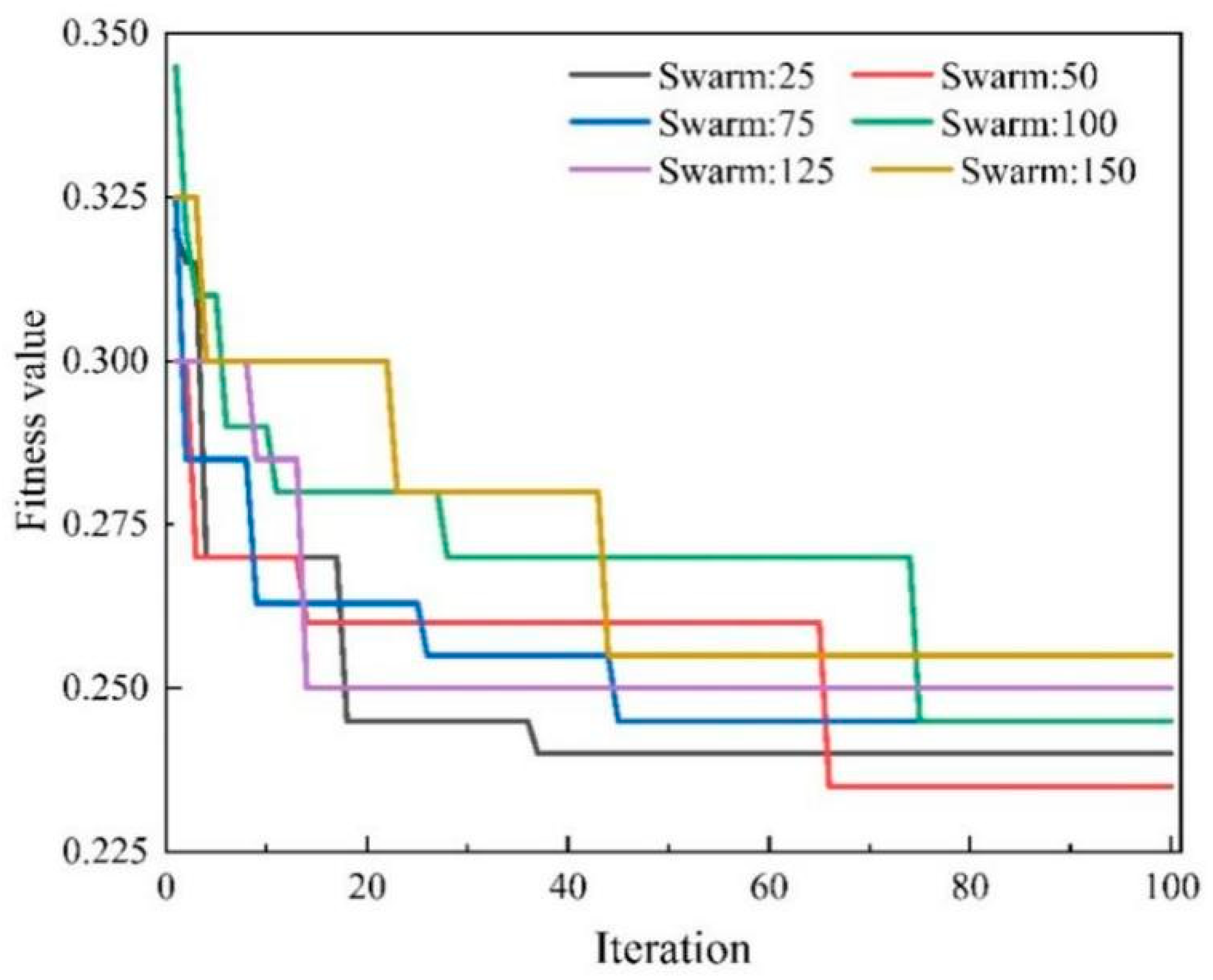
(4) Evaluation of the optimal prediction model. It is important to investigate a reliable WOA–RF model with optimal performance and optimal population size. To obtain the optimal population size, 6 different population sizes (25, 50, 75, 100, 125, 150) were selected and used in the model development process. Figure 6 shows the optimal fitting curve of the WOA–RF model under different population values. It shows the variation in population values with the increase in the number of iterations. The fitted values of the 6 fitted curves generated by the WOA–RF model tend to stabilize at 75 iterations. The WOA–RF hybrid model with different swarm sizes had the same performances in the training and testing sets according to accuracy, kappa, and MCC. The WOA–RF model received an accuracy of 0.9167, a kappa of 0.8846, and an MCC of 0.8932.
4.3. Comparison with Other Machine Learning Models
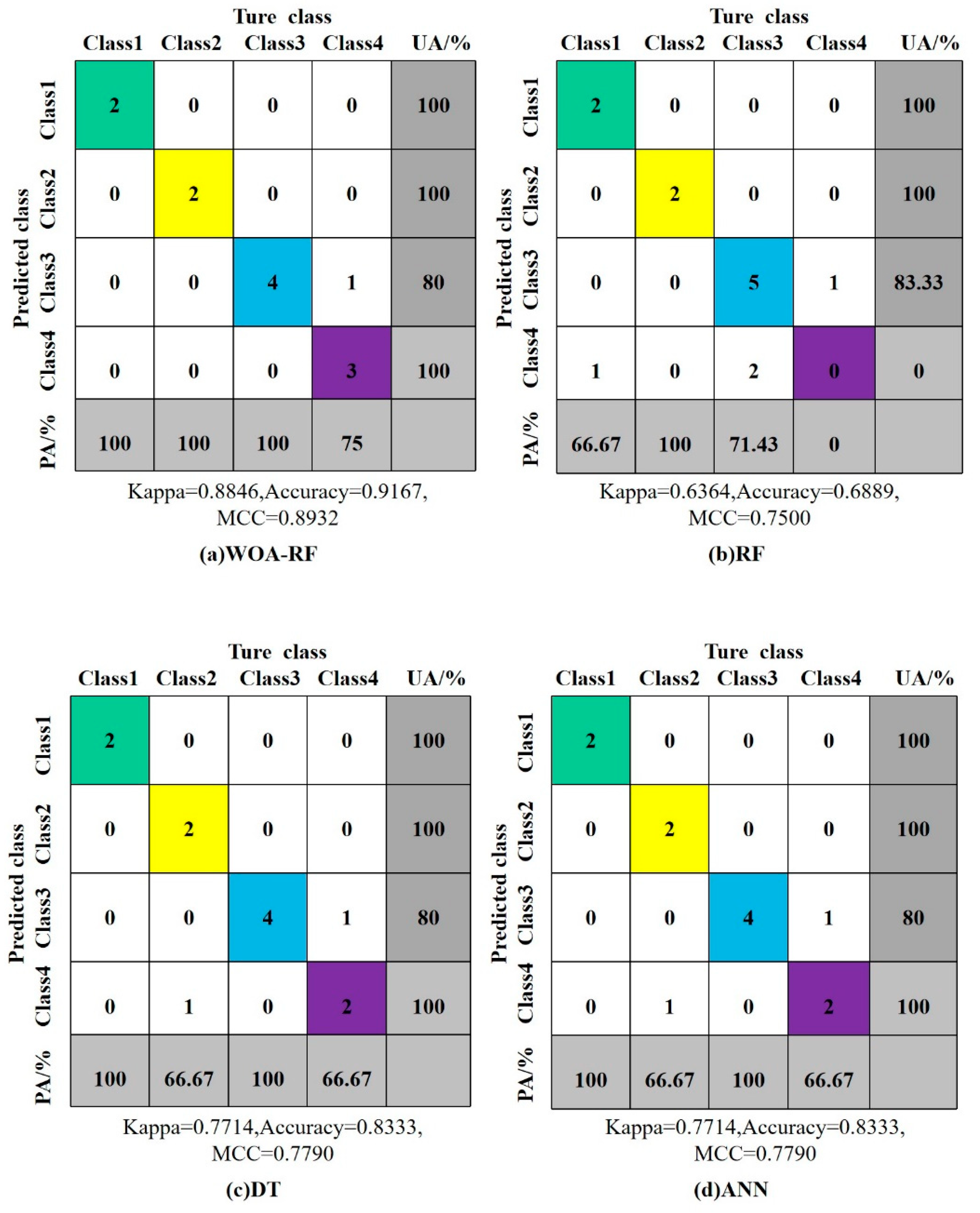
The WOA–RF hybrid model was tested and verified by testing datasets. According to the most commonly used split ratios of 80% and 20%, the total datasets were divided into 80% of training datasets and 20% of testing datasets; 20% of testing datasets were randomly selected from the total sample datasets, and the testing datasets had not been preprocessed and trained. This paper analyzed and compared different models from the perspectives of the confusion matrix, performance evaluation indicators, and other evaluation indicators. Based on the five evaluation indicators of the confusion matrix, accuracy, precision, recall, ROC, and AUC, the performance of different models can be measured. To test the accuracy of the WOA–RF, other models (RF, DT, ANN, KNN, and SVM) were used to classify and compare the same sample data of backfilling pipeline risk prediction. Figure 7 shows that compared with the RF, DT, ANN, KNN, and SVM classification models, the classification results of the WOA–RF hybrid model showed better performance. The accuracy of the RF, DT, ANN, KNN, and SVM classification models are 0.689, 0.500, 0.833, 0.500, and 0.750, respectively. Moreover, the kappa values from large to small are: 0.8846 (WOA–RF), 0.7714 (DT), 0.7714 (ANN), 0.6604 (SVM), 0.6364 (RF), and 0.3628 (KNN), and the MCC values from large to small are: 0.8932 (WOA–RF), 0.7790 (DT), 0.6364 (SVM), and 0.3628 (SVM), respectively. The WOA–RF hybrid model has the highest accuracy, with an accuracy of 0.917. In addition, the correct number of classified cases can also be obtained from the main diagonal of the confusion matrix. The numbers in the upper diagonal and lower diagonal areas represent the number of classified cases with errors.
Figure 8 represents the actual and predicted classification results on the training and testing datasets. Fifty-nine samples of the training and testing datasets were on the horizontal axis. The training set was distributed with 47 samples and the testing set with 12 samples. The categories of the samples are presented on the vertical axis. Figure 8 shows the training set samples without error samples; testing set sample 55 with an actual category of 4, which was misclassified as a category of 3; and the training and testing datasets with error rates of 0 and 9.09%, respectively. However, many training and testing samples of the other five models were wrongly classified. Therefore, the WOA–RF hybrid model performs better and with higher accuracy in predicting the invalidation risk prediction of backfilling pipelines.
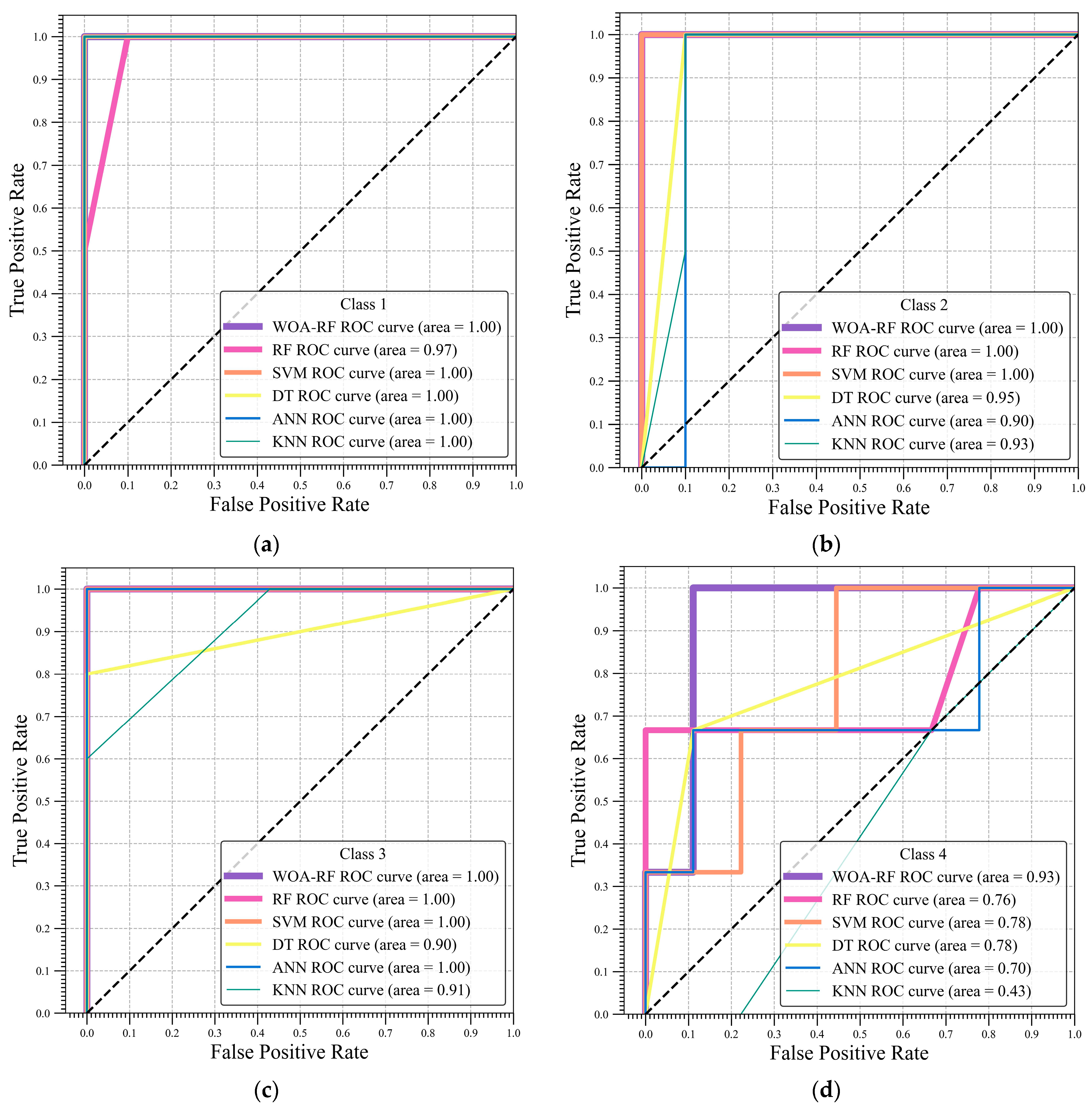
The test performance of different classification models on the invalidation risk of a backfilling pipeline is listed in Table 3. According to Table 3, the WOA–RF model has better prediction performance, and its model has the best precision, recall, and F1-score. Therefore, the WOA–RF model is a better classification model for invalidation risk prediction of backfilling pipelines. The ROC curve and AUC value of different individual classifications of different categories are shown in Figure 9. Figure 9 shows that the WOA–RF, RF, and SVM models performed similarly in Category 1 prediction and were superior to the DT, ANN, and KNN models; the WOA–RF and RF models performed similarly in Category 2 prediction and were superior to the DT, ANN, KNN, and SVM models; the WOA–RF, RF, ANN, and SVM models performed similarly in Category 3-based prediction and were superior to the DT and KNN models; and the WOA–RF model was superior to the RF, DT, ANN, KNN, and SVM models in Category 4 prediction. Therefore, the results in Figure 9 show that the WOA–RF model is a better classification model for invalidation risk prediction of backfilling pipelines.
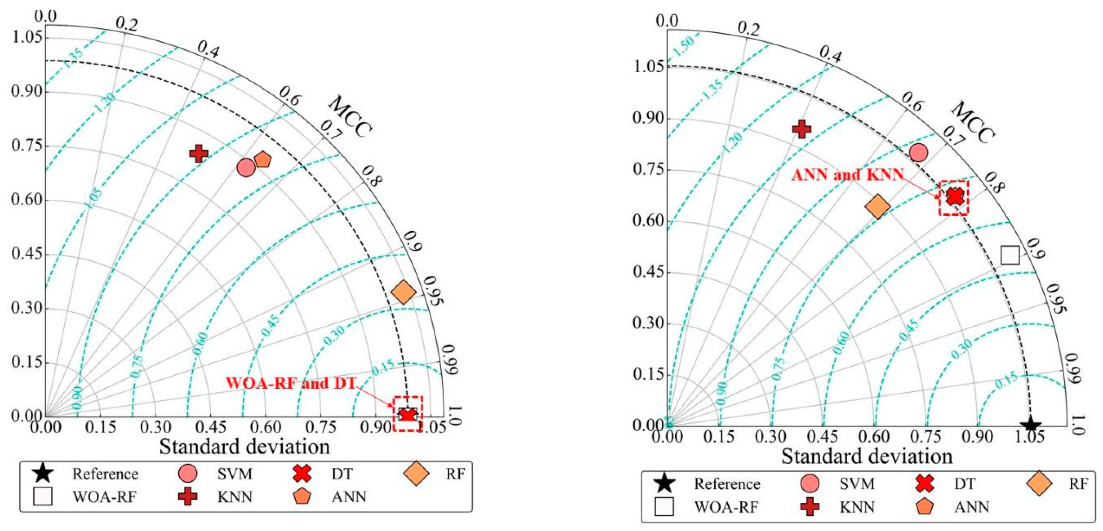
Additionally, the training datasets and testing datasets of six models (the WOA–RF, RF, DT, ANN, KNN, and SVM models) were compared and analyzed by using the Taylor chart. The results are shown in Figure 10. Figure 10 shows that the WOA–RF model was superior to the other models in the training datasets and testing datasets.
4.4. Sensitivity Analysis of Predictor Variables
To accurately predict the failure risk level of backfilling pipelines, the relationship and influence of various influencing factors should be comprehensively considered and evaluated [60,61,62,63]. Eight influencing factors (volume fraction of backfilling slurry, density of backfilling slurry, internal diameter of the pipeline, deviation rate, pipeline absolute roughness, stowing gradient, ratio of slurry flow rate with critical velocity, and weighted average particle size) were used for evaluation, all of which would have a certain impact on the risk prediction of backfilling pipelines. Further study on the importance of each influencing variable is needed.
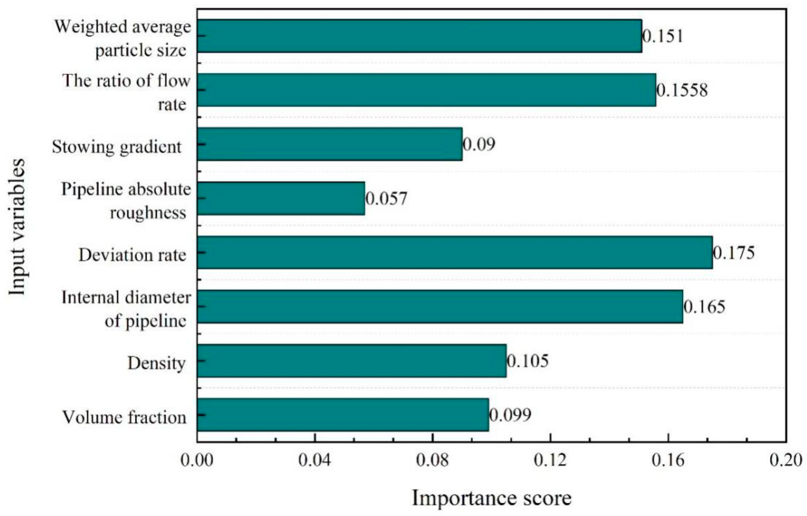
Figure 11 shows the importance score of influencing variables on the backfilling pipeline invalidation risk. The horizontal coordinate is the weight coefficient of each input factor, and the vertical coordinate is the English representation of the eight input factors. Obviously, according to the analysis in Figure 10, the deviation rate, the ratio of slurry flow rate with critical velocity, and weighted average particle size were the most important factors in the WOA–RF model, and the average particle size and internal diameter of the pipeline are sensitive variables affecting the risk grade prediction of backfilling the pipeline, accounting for 0.175, 0.1558, 0.151, and 0.165 of the total variables, respectively. It accounted for more than two-thirds of the importance score for all variables. The importance scores of the variables affecting the prediction of the failure risk grade of a backfilling pipeline were ranked in descending order: deviation rate (0.175) > internal diameter of the pipeline (0.165) > ratio of slurry flow rate with critical velocity (0.1558) > weighted average particle size (0.151) > density of backfilling slurry (0.105) > volume fraction of backfilling slurry (0.099) > stowing gradient (0.09) > pipeline absolute roughness (0.057). It can be seen from Figure 10 that most of the influencing variables have importance scores, and these influence variables are the basic input parameters of most engineering projects. In addition, different importance scores may be obtained when different datasets and classification models are adopted. More representative results can be obtained as more effective backfilling pipeline invalidation risk level cases become available in the future.
4.5. Engineering Validation
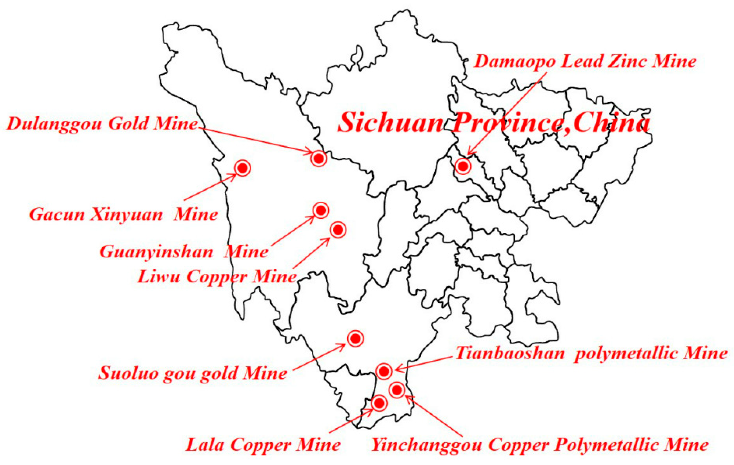
The WOA–RF hybrid model was applied to predict the invalidation risk level of the backfilling pipeline of nine actual mines in Sichuan, China, including Sichuan Xinyuan Gacun Mine, Danba Dulanggou Gold Mine, Sichuan Soluogou Gold Mine, Huili Lala Copper Mine, Liwu Copper Mine, Damaopo Lead Zinc Mine, Huidong Yinchanggou Copper Polymetallic Mine, Guanyinshan Lead Zinc Polymetallic Mine, and Huili Tianbaoshan Copper Lead Zinc Polymetallic Mine. Figure 12 shows the locations of the nine metal mines. To maximize the recovery of metal mine resources, the nine metal mines have adopted the backfilling method for mining, and their backfilling pipelines run the risk of pipeline leakage, burst, blockages, wear, etc. Long-term follow-up research on the backfilling pipelines of the mines by on-site technicians and sample data of the failure risk level of the backfilling pipes of these mines have been obtained. Table 4 shows that the relevant parameters are used to predict the invalidation risk level of the backfilling pipelines. Then, the WOA–RF model is used for prediction analysis, and the prediction results are also shown in Table 4. The prediction results show that the WOA–RF model is scientific and reasonable, has certain promotion and application value, and has good engineering practicability.
5. Study Limitations
Although the WOA–RF hybrid model achieved good results in the failure risk prediction of backfilling pipelines, some study limitations should be addressed in the future. For example, the influencing factors to consider the failure risk of backfilling pipelines are limited. In actual mining engineering, the influencing factors are more difficult to count and obtain accurately. In addition, the predictive performance of a single classification model is lower than that of a hybrid classification model. For this kind of prediction problem, other high-performance models can be adopted to build more complex models in the future. Meanwhile, the prediction accuracy of the model can be greatly improved by introducing an appropriate optimization algorithm. In addition, the classification accuracy of the optimized model can be further improved, and the generalization error of the hybrid model can be reduced by extending the database of the invalidation risk of backfilling pipelines and using the data enhancement algorithm.
6. Conclusions
In this paper, an optimized whale optimization algorithm and random forest hybrid model was proposed. Based on fifty-nine mine cases, the possibility of backfilling pipeline failure risk was evaluated. The dataset was randomly divided into a training set and testing set for model development and model verification, respectively. The WOA–RF hybrid model was established to classify the backfilling pipeline failure risk. Compared with other classification models (random forest, decision tree, artificial neural network, k-nearest neighbor, and support vector machine), the main research results are as follows:
(1) The WOA–RF model has the highest accuracy, with an accuracy of 0.917, showing that the WOA–RF model has a good classification effect and is also a better ML classifier for backfilling pipeline risk prediction.
(2) The sensitivity analysis of predictive variables shows that the deviation rate is the most important influencing factor. The ratio of the slurry flow rate to the critical velocity, weighted average particle size, and internal diameter of the pipeline are the most sensitive variables that affect the prediction of the backfilling pipeline risk level.
(3) The WOA–RF hybrid model was used to verify the failure risk of backfilling pipelines in nine actual mines in Sichuan, China. The predicted results were consistent with the failure cases of backfilling pipelines in the field investigation.
Author Contributions
Conceptualization, W.L. and Z.L. (Zhixiang Liu); methodology, W.L.; software, Z.L. (Zida Liu); validation, W.L. and Z.L. (Zhixiang Liu); formal analysis, W.L. and S.X.; investigation, W.L. and S.Z.; resources, Z.L. (Zhixiang Liu); data curation, W.L.; writing—original draft preparation, W.L.; writing—review and editing, Z.L. (Zhixiang Liu) and Z.L. (Zida Liu); visualization, Z.L. (Zhixiang Liu); supervision, Z.L. (Zhixiang Liu); project administration, Z.L. (Zhixiang Liu); funding acquisition, Z.L. (Zhixiang Liu). All authors have read and agreed to the published version of the manuscript.
Funding
This research project was supported by the National Natural Science Foundation of China (No. 41972283).
Data Availability Statement
Not applicable.
Acknowledgments
The authors would like to acknowledge the anonymous reviewers for their professional comments and constructive suggestions regarding improvements to the manuscript.
Conflicts of Interest
The authors declare no conflict of interest.
Nomenclature
| RF | random forest |
| DT | decision tree |
| ANN | artificial neural network |
| AI | artificial intelligence |
| HDD | Horizontal directional drilling |
| GWO | grey wolf optimizer |
| ACOA | ant colony optimization |
| MCC | Matthews correlation coefficient |
| ROC | the receiver operating characteristic |
| TN | true negative rate |
| FP | false positive |
| FPR | false positive rate |
| TOPSIS | technique for order preference by similarity to an ideal solution methods |
| WOA | whale optimization algorithm |
| SVM | support vector machine |
| KNN | k-nearest neighbor |
| ML | machine learning |
| ANFIS | adaptive neural fuzzy reasoning system |
| BAYES | bayes classifier |
| PSO | particle swarm optimization |
| IAHP | interval-based AHP |
| AUC | area under curve |
| TP | true positive rate |
| TPR | true positive rate |
| N | the number of the samples |
References
- Aljaroudi, A.; Thodi, P.; Akinturk, A.; Khan, F.; Paulin, M. Application of Probabilistic Methods for Predicting the Remaining Life of Offshore Pipelines. In Proceedings of the 2014 10th International Pipeline Conference, Calgary, AB, Canada, 29 September–3 October 2014. [Google Scholar]
- Aljaroudi, A.; Khan, F.; Akinturk, A.; Haddara, M.; Thodi, P. Probability of Detection and False Detection for Subsea Leak Detection Systems: Model and Analysis. J. Fail. Anal. Prev. 2015, 15, 873–882. [Google Scholar] [CrossRef]
- Kim, S. Inverse Transient Analysis for a Branched Pipeline System with Leakage and Blockage Using Impedance Method. Procedia Eng. 2014, 89, 1350–1357. [Google Scholar] [CrossRef] [Green Version]
- Aljaroudi, A.; Khan, F.; Akinturk, A.; Haddara, M.; Thodi, P. Risk assessment of offshore crude oil pipeline failure. J. Loss Prev. Process Ind. 2015, 37, 101–109. [Google Scholar] [CrossRef]
- Zhou, Y.; Hu, G.; Li, J.; Diao, C. Risk assessment along the gas pipelines and its application in urban planning. Land Use Policy 2014, 38, 233–238. [Google Scholar] [CrossRef]
- Tabesh, A.; Najafi, M.; Kohankar, Z.; Mohammadi, M.M.; Ashoori, T. Risk Identification for Pipeline Installation by Horizontal Directional Drilling (HDD). In Proceedings of the Pipelines 2019, Nashville, TN, USA, 21–24 July 2019; pp. 141–150. [Google Scholar]
- Pillay, A. Pipeline Risk Mitigation Study. In Proceedings of the 2002 4th International Pipeline Conference, Calgary, AB, Canada, 29 September–3 October 2002; pp. 769–779. [Google Scholar]
- Yang, Y.; Khan, F.; Thodi, P.; Abbassi, R. Corrosion induced failure analysis of subsea pipelines. Reliab. Eng. Syst. Saf. 2017, 159, 214–222. [Google Scholar] [CrossRef]
- Lu, L.; Liang, W.; Zhang, L.; Zhang, H.; Lu, Z.; Shan, J. A comprehensive risk evaluation method for natural gas pipelines by combining a risk matrix with a bow-tie model. J. Nat. Gas Sci. Eng. 2015, 25, 124–133. [Google Scholar] [CrossRef]
- Zhang, S.; Sun, B.; Yan, L.; Wang, C. Risk identification on hydropower project using the IAHP and extension of TOPSIS methods under interval-valued fuzzy environment. Nat. Hazards 2012, 65, 359–373. [Google Scholar] [CrossRef]
- Shin, S.; Lee, G.; Ahmed, U.; Lee, Y.; Na, J.; Han, C. Risk-based underground pipeline safety management considering corrosion effect. J. Hazard. Mater. 2018, 342, 279–289. [Google Scholar] [CrossRef]
- Mazumder, R.K.; Salman, A.M.; Li, Y. Failure risk analysis of pipelines using data-driven machine learning algorithms. Struct. Saf. 2021, 89, 102047. [Google Scholar] [CrossRef]
- Li, X.; Zhang, Y.; Abbassi, R.; Khan, F.; Chen, G. Probabilistic fatigue failure assessment of free spanning subsea pipeline using dynamic Bayesian network. Ocean Eng. 2021, 234, 109323. [Google Scholar] [CrossRef]
- Yu, Q.Y.; Hou, L.; Li, Y.H.; Chai, C.; Yang, K.; Liu, J.Q. Pipeline Failure Assessment Based on Fuzzy Bayesian Network and AHP. J. Pipeline Syst. Eng. Pract. 2023, 14, 04022059. [Google Scholar] [CrossRef]
- Jayan, T.J.; Muthukumar, K.; Renjith, V.R.; George, P. The risk assessment of a crude oil pipeline using fuzzy and bayesian based bow-tie analysis. J. Eng. Res. 2021, 9. [Google Scholar]
- Shao, X.; Li, X.; Wang, L.; Fang, Z.; Zhao, B.; Liu, E.; Tao, Y.; Liu, L. Study on the Pressure-Bearing Law of Backfilling Material Based on Three-Stage Strip Backfilling Mining. Energies 2020, 13, 211. [Google Scholar] [CrossRef] [Green Version]
- Zhang, J.; Zhou, N.; Huang, Y.; Zhang, Q. Impact law of the bulk ratio of backfilling body to overlying strata movement in fully mechanized backfilling mining. J. Min. Sci. 2011, 47, 73. [Google Scholar] [CrossRef]
- Aslkhalili, A.; Shiri, H.; Zendehboudi, S. Probabilistic Assessment of Lateral Pipeline–Backfill–Trench Interaction. J. Pipeline Syst. Eng. Pract. 2021, 12, 04021034. [Google Scholar] [CrossRef]
- Shukla, H.; Piratla, K.R.; Atamturktur, S. Influence of Soil Backfill on Vibration-Based Pipeline Leakage Detection. J. Pipeline Syst. Eng. Pract. 2020, 11, 04019055. [Google Scholar] [CrossRef]
- Liu, B.; Jiang, Z.; Nie, W. Application of VMD in Pipeline Leak Detection Based on Negative Pressure Wave. J. Sens. 2021, 2021, 8699362. [Google Scholar] [CrossRef]
- Yang, K.; Zhao, X.; Wei, Z.; Zhang, J. Development overview of paste backfill technology in China’s coal mines: A review. Environ. Sci. Pollut. Res. 2021, 28, 67957–67969. [Google Scholar] [CrossRef]
- Jia, H.; Yan, B.; Yilmaz, E. A Large Goaf Group Treatment by means of Mine Backfill Technology. Adv. Civ. Eng. 2021, 2021, 3737145. [Google Scholar] [CrossRef]
- Qi, C.; Fourie, A.; Du, X.; Tang, X. Prediction of open stope hangingwall stability using random forests. Nat. Hazards 2018, 92, 1179–1197. [Google Scholar] [CrossRef]
- Lin, Y.; Zhou, K.; Li, J.L. Prediction of Slope Stability Using Four Supervised Learning Methods. IEEE Access 2018, 6, 31169–31179. [Google Scholar] [CrossRef]
- Armaghani, D.J.; Harandizadeh, H.; Momeni, E.; Maizir, H.; Zhou, J. An optimized system of GMDH-ANFIS predictive model by ICA for estimating pile bearing capacity. Artif. Intell. Rev. 2022, 55, 2313–2350. [Google Scholar] [CrossRef]
- Armaghani, D.J.; Yagiz, S.; Mohamad, E.T.; Zhou, J. Prediction of TBM performance in fresh through weathered granite using empirical and statistical approaches. Tunn. Undergr. Space Technol. 2021, 118, 104183. [Google Scholar] [CrossRef]
- Xu, C.; Wang, J.; Zheng, T.; Cao, Y.; Ye, F. Prediction of prognosis and survival of patients with gastric cancer by a weighted improved random forest model: An application of machine learning in medicine. Arch. Med. Sci. 2022, 18, 1208–1220. [Google Scholar] [PubMed]
- Khandelwal, M.; Monjezi, M. Prediction of Backbreak in Open-Pit Blasting Operations Using the Machine Learning Method. Rock Mech. Rock Eng. 2013, 46, 389–396. [Google Scholar] [CrossRef]
- Qi, C.; Tang, X. Slope stability prediction using integrated metaheuristic and machine learning approaches: A comparative study. Comput. Ind. Eng. 2018, 118, 112–122. [Google Scholar] [CrossRef]
- Ghalambaz, M.; Jalilzadeh Yengejeh, R.; Davami, A.H. Building energy optimization using Grey Wolf Optimizer (GWO). Case Stud. Therm. Eng. 2021, 27, 101250. [Google Scholar] [CrossRef]
- Goudos, S.K.; Zaharis, Z.D.; Baltzis, K.B. Particle Swarm Optimization as Applied to Electromagnetic Design Problems. Int. J. Swarm Intell. Res. 2018, 9, 47–82. [Google Scholar] [CrossRef]
- Naadimuthu, G.; Liu, D.M.; Lee, E.S. Application of an adaptive neural fuzzy inference system to thermal comfort and group technology problems. Comput. Math. Appl. 2007, 54, 1395–1402. [Google Scholar] [CrossRef] [Green Version]
- Zhang, B.J.; Yang, G.Q.; Xiong, B.L. BP Artificial Neural Network Study on Slop Stability. Appl. Mech. Mater. 2012, 170–173, 1243–1246. [Google Scholar] [CrossRef]
- Li, F.; Wang, W.; Xu, J.; Yi, J.; Wang, Q. Comparative study on vulnerability assessment for urban buried gas pipeline network based on SVM and ANN methods. Process Saf. Environ. Prot. 2019, 122, 23–32. [Google Scholar] [CrossRef]
- Mansour, A.M. Texture Classification using Naive Bayes Classifier. Int. J. Comput. Sci. Netw. Secur. 2018, 18, 112–120. [Google Scholar]
- Otero, F.E.B.; Freitas, A.A.; Johnson, C.G. Inducing decision trees with an ant colony optimization algorithm. Appl. Soft Comput. 2012, 12, 3615–3626. [Google Scholar] [CrossRef] [Green Version]
- Zhou, J.; Zhu, S.; Qiu, Y.; Armaghani, D.J.; Zhou, A.; Yong, W. Predicting tunnel squeezing using support vector machine optimized by whale optimization algorithm. Acta Geotech. 2022, 17, 1343–1366. [Google Scholar] [CrossRef]
- Liu, D.; Fan, Z.R.; Fu, Q.; Li, M.; Faiz, M.A.; Ali, S.; Li, T.X.; Zhang, L.L.; Khan, M.I. Random forest regression evaluation model of regional flood disaster resilience based on the whale optimization algorithm. J. Clean. Prod. 2020, 250, 119468. [Google Scholar] [CrossRef]
- Wang, X.M.; Gao, R.W.; Hu, W.; Feng, Y.; Zhou, D.H. Risk prediction model of filling pipeline blockage. J. Cent. South Univ. 2013, 44, 4604–4610. (In Chinese) [Google Scholar]
- Li, D.Y.; Liu, Z.D.; Xiao, P.; Zhou, J.; Armaghani, D.J. Intelligent rockburst prediction model with sample category balance using feedforward neural network and Bayesian optimization. Undergr. Space 2022, 7, 833–846. [Google Scholar] [CrossRef]
- Li, D.Y.; Liu, Z.D.; Armaghani, D.J.; Xiao, P.; Zhou, J. Novel ensemble intelligence methodologies for rockburst assessment in complex and variable environments. Sci. Rep. 2022, 12, 1844. [Google Scholar] [CrossRef]
- Li, D.Y.; Liu, Z.D.; Armaghani, D.J.; Xiao, P.; Zhou, J. Novel Ensemble Tree Solution for Rockburst Prediction Using Deep Forest. Mathematics 2022, 10, 787. [Google Scholar] [CrossRef]
- Speiser, J.L.; Miller, M.E.; Tooze, J.; Ip, E. A comparison of random forest variable selection methods for classification prediction modeling. Expert Syst. Appl. 2019, 134, 93–101. [Google Scholar] [CrossRef]
- Wang, Q.; Chen, H.H. Optimization of parallel random forest algorithm based on distance weight. J. Intell. Fuzzy Syst. 2020, 39, 1951–1963. [Google Scholar] [CrossRef]
- Daho, M.E.; Chikh, M.A. Combining Bootstrapping Samples, Random Subspaces and Random Forests to Build Classifiers. J. Med. Imaging Health Inform. 2015, 5, 539–544. [Google Scholar] [CrossRef]
- Byeon, H. Comparing the Accuracy and Developed Models for Predicting the Confrontation Naming of the Elderly in South Korea using Weighted Random Forest, Random Forest, and Support Vector Regression. Int. J. Adv. Comput. Sci. Appl. 2021, 12, 326–331. [Google Scholar] [CrossRef]
- Zhang, G.Q.; Hui, G.Y.; Yang, A.M.; Zhao, Z.H. A simple and effective approach to quantitatively characterize structural complexity. Sci. Rep. 2021, 11, 1326. [Google Scholar] [CrossRef] [PubMed]
- Ben Ayed, A.; Benhammouda, M.; Ben Halima, M.; Alimi, A. Random Forest Ensemble Classification Based Fuzzy Logic; SPIE: Washington, DC, USA, 2017; Volume 10341. [Google Scholar]
- Mirjalili, S.; Lewis, A. The Whale Optimization Algorithm. Adv. Eng. Softw. 2016, 95, 51–67. [Google Scholar] [CrossRef]
- Mirjalili, S.; Mirjalili, S.M.; Saremi, S.; Mirjalili, S. Whale Optimization Algorithm: Theory, Literature Review, and Application in Designing Photonic Crystal Filters. In Nature-Inspired Optimizers: Theories, Literature Reviews and Applications; Mirjalili, S., Song Dong, J., Lewis, A., Eds.; Springer International Publishing: Cham, Switzerland, 2020; pp. 219–238. [Google Scholar]
- Luo, J.; Shi, B.Y. A hybrid whale optimization algorithm based on modified differential evolution for global optimization problems. Appl. Intell. 2019, 49, 1982–2000. [Google Scholar] [CrossRef]
- Liang, X.D.; Xu, S.W.; Liu, Y.; Sun, L.L. A Modified Whale Optimization Algorithm and Its Application in Seismic Inversion Problem. Mob. Inf. Syst. 2022, 2022, 9159130. [Google Scholar] [CrossRef]
- Perez, I.M.; Airola, A.; Bostrom, P.J.; Jambor, I.; Pahikkala, T. Tournament leave-pair-out cross-validation for receiver operating characteristic analysis. Stat. Methods Med. Res. 2019, 28, 2975–2991. [Google Scholar] [CrossRef]
- Hand, D.J.; Till, R.J. A simple generalisation of the area under the ROC curve for multiple class classification problems. Mach. Learn. 2001, 45, 171–186. [Google Scholar] [CrossRef]
- Mourão, M.F.; Braga, A.C. Strengths and Weaknesses of Three Software Programs for the Comparison of Systems Based on ROC Curves; Springer: Cham, Switzerland, 2016; pp. 359–372. [Google Scholar]
- Pu, Y.Y.; Apel, D.; Xu, H.W. A Principal Component Analysis/Fuzzy Comprehensive Evaluation for Rockburst Potential in Kimberlite. Pure Appl. Geophys. 2018, 175, 2141–2151. [Google Scholar] [CrossRef]
- Zhou, J.; Li, X.; Mitri, H.S. Classification of Rockburst in Underground Projects: Comparison of Ten Supervised Learning Methods. J. Comput. Civ. Eng. 2016, 30, 04016003. [Google Scholar] [CrossRef]
- Zhou, J.; Qiu, Y.G.; Khandelwal, M.; Zhu, S.L.; Zhang, X.L. Developing a hybrid model of Jaya algorithm-based extreme gradient boosting machine to estimate blast-induced ground vibrations. Int. J. Rock Mech. Min. Sci. 2021, 145, 104856. [Google Scholar] [CrossRef]
- Chou, J.-S.; Lin, C. Predicting Disputes in Public-Private Partnership Projects: Classification and Ensemble Models. J. Comput. Civ. Eng. 2013, 27, 51–60. [Google Scholar] [CrossRef]
- Zhou, J.; Dai, Y.; Khandelwal, M.; Monjezi, M.; Yu, Z.; Qiu, Y. Performance of Hybrid SCA-RF and HHO-RF Models for Predicting Backbreak in Open-Pit Mine Blasting Operations. Nat. Resour. Res. 2021, 30, 4753–4771. [Google Scholar] [CrossRef]
- Zhang, J.; Huang, Y.; Ma, G.; Yuan, Y.; Nener, B. Automating the mixture design of lightweight foamed concrete using multi-objective firefly algorithm and support vector regression. Cem. Concr. Compos. 2021, 121, 104103. [Google Scholar] [CrossRef]
- Liu, Z.; Armaghani, D.J.; Fakharian, P.; Li, D.; Ulrikh, D.V.; Orekhova, N.N.; Khedher, K.M. Rock Strength Estimation Using Several Tree-Based ML Techniques. Comput. Model. Eng. Sci. 2022, 133, 799–824. [Google Scholar] [CrossRef]
- Pu, Y.; Apel, D.B.; Xu, H. Rockburst prediction in kimberlite with unsupervised learning method and support vector classifier. Tunn. Undergr. Space Technol. 2019, 90, 12–18. [Google Scholar] [CrossRef]
Figure 1.
The location distribution of 59 metal mines.

Figure 2.
Backfilling pipeline failure photos: (a) pipeline blockages; (b) pipeline wear; (c) pipeline leakage; (d) pipeline burst.
Figure 2.
Backfilling pipeline failure photos: (a) pipeline blockages; (b) pipeline wear; (c) pipeline leakage; (d) pipeline burst.

Figure 3.
The correlation coefficient matrix of backfilling pipeline failure risk database.

Figure 4.
Confusion matrix and performance indexes.

Figure 5.
The whole analysis process of the WOA–RF hybrid classifier model.

Figure 6.
Optimization of the WOA–RF model with different population values.

Figure 7.
The confusion matrix.


Figure 8.
The classification results on training and testing datasets of the WOA–RF model.

Figure 9.
ROC curves and AUC values for different individual classifiers: (a) extremely dangerous; (b) significant risk; (c) greater risk; (d) general risk.
Figure 9.
ROC curves and AUC values for different individual classifiers: (a) extremely dangerous; (b) significant risk; (c) greater risk; (d) general risk.

Figure 10.
Taylor graph training datasets, testing datasets.

Figure 11.
Importance score of influencing variables on the backfilling pipeline invalidation risk.

Figure 12.
The locations of the nine metal mines.


Table 1.
The assessment criteria for the failure risk level of the backfilling pipeline.
| Volume Fraction of Backfilling Slurry I1/% | Density of Backfilling Slurry I2/t.m−3 | The Internal Diameter of the Pipeline I3/mm | The Deviation Rate I4/% | Pipeline Absolute Roughness I5/um | Stowing Gradient I6 | The Ratio of Slurry Flow Rate with the Critical Velocity I7 | Weighted Average Particle Size I8/mm | Risk Level |
|---|---|---|---|---|---|---|---|---|
| ≥50 | ≥1.9 | ≤100 | ≥5 | ≥500 | ≥7 | ≤1 | ≥2.5 | 1 |
| ≥40~<50 | ≥1.7~<1.9 | >100~≤150 | ≥3~<5 | ≥300~<500 | ≥5~<7 | >1~≤1.2 | ≥0.7~<2.5 | 2 |
| ≥30~<40 | ≥1.5~<1.7 | >150~≤200 | ≥1~<3 | ≥100~<300 | ≥3~<5 | >1.2~≤1.5 | ≥0.3~<0.7 | 3 |
| <30 | <1.5 | >200 | <1 | <100 | ≥1~<3 | <1.5 | <0.3 | 4 |
Table 2.
The statistical information of backfilling pipeline invalidation risk influence factors and level.
Table 2.
The statistical information of backfilling pipeline invalidation risk influence factors and level.
| Sample of Filling Pipeline | Volume Fraction of Filling Slurry I1/% | Density of Filling Slurry I2/t.m−3 | Internal Diameter of the Pipeline I3/mm | Deviation Rate I4/% | Pipeline Absolute Roughness I5/um | Stowing Gradient I6 | The Ratio of Slurry Flow Rate with the Critical Velocity I7 | Weighted Average Particle Size I8/mm | Risk Level |
|---|---|---|---|---|---|---|---|---|---|
| 1 | 56 | 1.98 | 199 | 2.72 | 300 | 3.8 | 1.30 | 0.58 | 2 |
| 2 | 33 | 1.69 | 160 | 0.98 | 500 | 9.6 | 3.00 | 0.05 | 3 |
| 3 | 24 | 1.68 | 82 | 0.56 | 100 | 5.2 | 1.60 | 0.21 | 4 |
| 4 | 52 | 1.94 | 107 | 1.27 | 200 | 5.8 | 3.50 | 0.11 | 3 |
| 5 | 60 | 1.92 | 104 | 1.01 | 300 | 3.5 | 3.20 | 0.05 | 3 |
| 6 | 30 | 1.76 | 69 | 2.65 | 200 | 3.2 | 1.50 | 0.05 | 4 |
| 7 | 60 | 1.68 | 69 | 1.03 | 100 | 5 | 1.57 | 0.25 | 3 |
| 8 | 56 | 1.77 | 120 | 0.69 | 300 | 3 | 1.60 | 0.13 | 3 |
| 9 | 28 | 1.86 | 65 | 1.65 | 200 | 6.8 | 1.62 | 0.65 | 4 |
| 10 | 68 | 1.78 | 148 | 1.58 | 100 | 4.7 | 1.66 | 0.05 | 3 |
| 11 | 51 | 1.93 | 152 | 1.23 | 300 | 4.1 | 1.13 | 0.26 | 2 |
| 12 | 27 | 1.49 | 79 | 2.41 | 100 | 4.7 | 1.39 | 0.17 | 4 |
| 13 | 55 | 1.77 | 120 | 0.69 | 300 | 3 | 1.60 | 0.13 | 3 |
| 14 | 43 | 1.73 | 170 | 1.37 | 200 | 6.6 | 1.72 | 0.19 | 3 |
| 15 | 51 | 1.97 | 158 | 1.74 | 300 | 7.8 | 1.30 | 0.21 | 2 |
| 16 | 26 | 1.89 | 72 | 1.37 | 100 | 5.4 | 1.43 | 0.24 | 4 |
| 17 | 57 | 1.99 | 197 | 2.71 | 300 | 3.7 | 1.30 | 0.55 | 2 |
| 18 | 34 | 1.71 | 154 | 0.99 | 500 | 9.5 | 3.00 | 0.07 | 3 |
| 19 | 22 | 1.64 | 78 | 0.54 | 100 | 5.3 | 1.60 | 0.19 | 4 |
| 20 | 51 | 1.91 | 104 | 1.25 | 200 | 5.9 | 3.50 | 0.13 | 3 |
| 21 | 61 | 1.94 | 108 | 1.03 | 300 | 3.6 | 3.20 | 0.03 | 3 |
| 22 | 56 | 1.71 | 71 | 2.61 | 200 | 3.3 | 1.50 | 0.04 | 4 |
| 23 | 59 | 1.73 | 71 | 1.01 | 100 | 5.1 | 1.57 | 0.26 | 3 |
| 24 | 55 | 1.81 | 118 | 0.72 | 300 | 3.2 | 1.60 | 0.15 | 3 |
| 25 | 27 | 1.81 | 67 | 1.63 | 200 | 6.9 | 1.62 | 6.47 | 4 |
| 26 | 64 | 1.75 | 151 | 1.61 | 100 | 4.5 | 1.66 | 0.04 | 3 |
| 27 | 53 | 1.77 | 121 | 0.69 | 300 | 3.1 | 1.56 | 0.14 | 3 |
| 28 | 61 | 1.71 | 149 | 1.58 | 100 | 4.3 | 1.63 | 0.05 | 3 |
| 29 | 52 | 1.91 | 201 | 2.66 | 300 | 3.5 | 1.35 | 0.56 | 2 |
| 30 | 30 | 1.69 | 161 | 1.02 | 500 | 9.3 | 3.05 | 0.08 | 3 |
| 31 | 56 | 1.98 | 199 | 2.72 | 300 | 3.2 | 1.30 | 0.24 | 2 |
| 32 | 33 | 1.69 | 160 | 0.98 | 500 | 9.6 | 3.00 | 0.43 | 3 |
| 33 | 24 | 1.68 | 82 | 0.56 | 100 | 5.2 | 1.60 | 0.08 | 3 |
| 34 | 52 | 1.94 | 107 | 1.27 | 200 | 5.8 | 3.50 | 0.16 | 3 |
| 35 | 62 | 1.97 | 152 | 4.6 | 300 | 2.9 | 1.83 | 0.62 | 2 |
| 36 | 54 | 1.76 | 179 | 1.25 | 100 | 4.8 | 2.52 | 0.08 | 3 |
| 37 | 31 | 1.78 | 148 | 1.58 | 200 | 4.7 | 1.66 | 0.05 | 4 |
| 38 | 57 | 1.78 | 168 | 1.5 | 200 | 4.2 | 1.80 | 0.62 | 2 |
| 39 | 58 | 1.69 | 145 | 0.91 | 500 | 9.6 | 3.20 | 0.08 | 3 |
| 40 | 59 | 1.83 | 69 | 1.65 | 100 | 6.7 | 1.50 | 0.52 | 2 |
| 41 | 56 | 1.92 | 98 | 1.19 | 200 | 5.8 | 3.50 | 0.11 | 3 |
| 42 | 56 | 1.92 | 104 | 1.01 | 300 | 3.8 | 3.30 | 0.06 | 4 |
| 43 | 67 | 1.71 | 72 | 2.67 | 200 | 3.5 | 1.70 | 0.05 | 3 |
| 44 | 58 | 1.68 | 78 | 1.18 | 100 | 5.2 | 1.60 | 0.28 | 2 |
| 45 | 69 | 1.32 | 218 | 1.12 | 156 | 6.1 | 2.34 | 0.02 | 1 |
| 46 | 68 | 1.06 | 274 | 1.65 | 178 | 6.9 | 1.08 | 0.23 | 1 |
| 47 | 27 | 1.89 | 165 | 4.16 | 145 | 1.3 | 1.15 | 0.07 | 3 |
| 48 | 64 | 1.27 | 203 | 3.49 | 139 | 6.4 | 1.07 | 0.11 | 1 |
| 49 | 36 | 1.55 | 229 | 1.93 | 170 | 5.4 | 1.16 | 0.03 | 2 |
| 50 | 30 | 1.24 | 240 | 1.72 | 246 | 7.2 | 1.19 | 0.04 | 1 |
| 51 | 25 | 1.91 | 221 | 2.71 | 423 | 3.0 | 3.41 | 0.18 | 4 |
| 52 | 66 | 1.13 | 192 | 1.57 | 124 | 6.5 | 1.58 | 0.02 | 1 |
| 53 | 28 | 1.26 | 206 | 1.88 | 152 | 6.7 | 1.03 | 0.05 | 2 |
| 54 | 67 | 1.32 | 250 | 1.34 | 161 | 6.7 | 2.15 | 0.09 | 1 |
| 55 | 65 | 1.05 | 234 | 1.27 | 194 | 7.0 | 1.87 | 0.03 | 1 |
| 56 | 27 | 1.78 | 219 | 6.55 | 382 | 4.4 | 1.43 | 0.04 | 4 |
| 57 | 60 | 0.99 | 93 | 1.60 | 194 | 7.0 | 1.05 | 0.01 | 1 |
| 58 | 63 | 1.20 | 207 | 5.16 | 247 | 7.1 | 2.94 | 0.05 | 1 |
| 59 | 64 | 1.58 | 212 | 1.24 | 189 | 6.1 | 1.14 | 0.01 | 1 |
Table 3.
Testing performance of different classifiers for the invalidation risk of the backfilling pipeline problem: extremely dangerous (Class 1), significant risk (Class 2), greater risk (Class 3), and general risk (Class 4).
Table 3.
Testing performance of different classifiers for the invalidation risk of the backfilling pipeline problem: extremely dangerous (Class 1), significant risk (Class 2), greater risk (Class 3), and general risk (Class 4).
| Precision | Recall | F1-Score | Precision | Recall | F1-Score | ||
|---|---|---|---|---|---|---|---|
| WOA–RF | RF | ||||||
| class1 | 1.00 | 1.00 | 1.00 | class1 | 1.00 | 1.00 | 1.00 |
| class2 | 1.00 | 1.00 | 1.00 | class2 | 1.00 | 1.00 | 1.00 |
| class3 | 1.00 | 0.80 | 0.89 | class3 | 1.00 | 0.80 | 0.89 |
| class4 | 0.75 | 1.00 | 0.86 | class4 | 0.75 | 1.00 | 0.86 |
| DT | ANN | ||||||
| class1 | 1.00 | 1.00 | 1.00 | class1 | 1.00 | 1.00 | 1.00 |
| class2 | 0.67 | 1.00 | 0.80 | class2 | 0.67 | 1.00 | 0.80 |
| class3 | 1.00 | 0.80 | 0.89 | class3 | 1.00 | 0.80 | 0.89 |
| class4 | 0.67 | 0.67 | 0.67 | class4 | 0.67 | 0.67 | 0.67 |
| KNN | SVM | ||||||
| class1 | 0.50 | 1.00 | 0.67 | class1 | 0.67 | 1.00 | 0.80 |
| class2 | 0.40 | 1.00 | 0.57 | class2 | 0.67 | 1.00 | 0.80 |
| class3 | 1.00 | 0.40 | 0.57 | class3 | 1.00 | 0.80 | 0.89 |
| class4 | 0.00 | 0.00 | 0.00 | class4 | 0.50 | 0.33 | 0.40 |
Table 4.
Application of the WOA–RF model in practical engineering.
| Engineering | Volume Fraction of Filling Slurry I1/% | Density of Filling Slurry I2/t.m−3 | Internal Diameter of the Pipeline I3/mm | Deviation Rate I4/% | Pipeline Absolute Roughness I5/um | Stowing Gradient I6 | The Ratio of Slurry Flow Rate with the Critical Velocity I7 | Weighted Average Particle Size I8/mm | Risk Level | Predicted Level |
|---|---|---|---|---|---|---|---|---|---|---|
| Gacun Xinyuan mine | 62 | 1.94 | 205 | 5.78 | 300 | 3.5 | 1.45 | 2.65 | 1 | 1 |
| Dulang gou gold mine | 30 | 1.32 | 74 | 1.37 | 100 | 5.6 | 1.47 | 0.25 | 4 | 4 |
| Guanyinshan mine | 57 | 1.85 | 150 | 3.71 | 400 | 6.7 | 1.10 | 0.75 | 2 | 2 |
| Liwu copper mine | 45 | 1.65 | 154 | 2.10 | 250 | 4.5 | 1.42 | 0.47 | 3 | 3 |
| Suoluo Gou gold mine | 28 | 1.45 | 215 | 0.54 | 85 | 5.3 | 1.60 | 0.19 | 4 | 4 |
| Huili Lala copper mine | 51 | 1.51 | 180 | 1.25 | 200 | 5.9 | 3.50 | 0.43 | 3 | 3 |
| Damaopo Lead Zinc Mine | 66 | 2.05 | 92 | 5.57 | 524 | 7.5 | 0.78 | 2.00 | 1 | 1 |
| Tianbaoshan polymetallic Mine | 58 | 1.76 | 136 | 1.88 | 152 | 6.7 | 1.03 | 0.95 | 2 | 2 |
| Yinchanggou Copper mine | 68 | 1.98 | 90 | 1.34 | 512 | 6.7 | 2.15 | 3.09 | 1 | 1 |
Disclaimer/Publisher’s Note: The statements, opinions and data contained in all publications are solely those of the individual author(s) and contributor(s) and not of MDPI and/or the editor(s). MDPI and/or the editor(s) disclaim responsibility for any injury to people or property resulting from any ideas, methods, instructions or products referred to in the content. |
© 2023 by the authors. Licensee MDPI, Basel, Switzerland. This article is an open access article distributed under the terms and conditions of the Creative Commons Attribution (CC BY) license (https://creativecommons.org/licenses/by/4.0/).
Share and Cite
MDPI and ACS Style
Liu, W.; Liu, Z.; Liu, Z.; Xiong, S.; Zhang, S. Random Forest and Whale Optimization Algorithm to Predict the Invalidation Risk of Backfilling Pipeline. Mathematics 2023, 11, 1636. https://doi.org/10.3390/math11071636
AMA Style
Liu W, Liu Z, Liu Z, Xiong S, Zhang S. Random Forest and Whale Optimization Algorithm to Predict the Invalidation Risk of Backfilling Pipeline. Mathematics. 2023; 11(7):1636. https://doi.org/10.3390/math11071636
Chicago/Turabian StyleLiu, Weijun, Zhixiang Liu, Zida Liu, Shuai Xiong, and Shuangxia Zhang. 2023. "Random Forest and Whale Optimization Algorithm to Predict the Invalidation Risk of Backfilling Pipeline" Mathematics 11, no. 7: 1636. https://doi.org/10.3390/math11071636
Note that from the first issue of 2016, this journal uses article numbers instead of page numbers. See further details here.