
Structures of Critical Nontree Graphs with Cutwidth Four
1
School of Mathematics and Statistics, Huanghuai University, Zhumadian 463000, China
2
Department of Mathematics, West Virginia University, Morgantown, WV 26506, USA
*
Author to whom correspondence should be addressed.
Mathematics 2023, 11(7), 1631; https://doi.org/10.3390/math11071631
Submission received: 7 February 2023
/
Revised: 21 March 2023
/
Accepted: 23 March 2023
/
Published: 28 March 2023
(This article belongs to the Special Issue Graph Theory and Applications)
Abstract
:The cutwidth of a graph G is the smallest integer k () such that the vertices of G are arranged in a linear layout , in such a way that for each , there are at most k edges with one endpoint in and the other in . The cutwidth problem for G is to determine the cutwidth k of G. A graph G with cutwidth k is k-cutwidth critical if every proper subgraph of G has a cutwidth less than k and G is homeomorphically minimal. In this paper, except five irregular graphs, other 4-cutwidth critical graphs were resonably classified into two classes, which are graph class with a central vertex , and graph class with a central cycle of length , respectively, and any member of two graph classes can skillfuly achieve a subgraph decomposition with cardinality 2, 3 or 4, where each member of is either a 2-cutwith graph or a 3-cutwidth graph.
1. Introduction
The graphs under consideration in this paper are finite, simple and connected, and for the undefined graph-theoretic terminologies, we refer the reader to the book by Bondy and Murty [1]. The cutwidth of a graph G is the smallest integer k (), such that the vertices of G are arranged in a linear layout , in such a way that for each , there are at most k edges with one endpoint in and the other in . The method used to compute the optimum cutwidth of a graph G is usually referred to as the cutwidth minimization problem, and has received an enormous amount of interest in graph theory literature [2] since the 1950s. From [3,4,5,6], for a graph G and a nonnegative integer k, deciding whether the cutwidth value of graph G is less than k is an NP-complete problem for general graphs except for trees, and it remains to be -complete even though G is planar with a maximum vertex degree of 3, by [7]. Therefore, most of previous investigations of the cutwidth problem have been mainly concentrated on polynomial time approximation algorithms for general graphs, and on polynomial time algorithms for special graphs for solving their cutwidth [2,4,5]. Despite these theoretical algorithms of the cutwidth minimization problem, research on studying the structural properties of the extreme (or critical) graph classes whose cutwidth is a given integer value have been paid little attention. As far as we know, the 2-cutwidth graph class has five forbidden subgraphs – [8] (see Figure 1 below), the family of 3-cutwidth trees possesses 18 forbidden subtrees [9], and 50 forbidden subgraphs of unicyclic graphs with cutwidth 3 were also found by [10]. As for the inner structures of the critical graphs with cutwidth k, ref. [11] found that any critical tree with cutwidth value k can be decomposed into three -cutwidth subtrees which are either edge-joint or edge-disjoint. Recently, the decomposability of a class of special k-cutwidth critical graphs with a central vertex and at least two cut edges and was also characterized by [12]. However, for general critical graphs with cutwidth , their inner structural properties are unfortunately not yet known. The cutwidth minimization problem for graphs has many significant applications. In the early 1970s, Adolphson and Hu used it to model the number of channels in the optimum layout of a circuit [13]. Other applications of this problem include circuits’ layout [14,15], automatic graph drawing [16], network reliability [17], information retrieval [18], urban drainage network design [19] and others. In particular, the cutwidth is closely connected to a basic parameter called the congestion, in designing microchip circuits and micro communication element system [2,20,21]. Herein, a graph G is considered to be a mathematical model of the wiring diagram of an electronic circuit, in which the vertices of G mean components and the edges of G represent wires connecting these vertices. When a circuit is embedded into a certain architecture (say, a path or a cycle ), the largest number of overlapping wires is referred to as the congestion, which is one of the key parameters determining the electronic performance. These are of great interest to scholars investigating the cutwidth problem in graph theory practically. Theoretically, the cutwidth problem is also closely bound up with other graph parameters such as bandwidth, modified bandwidth, pathwidth and treewidth [2,22,23]. For example, this is the case for any graph G with vertices of a degree bound by an integer , , where and are cutwidth value and pathwidth value, respectively. In this paper, by virtue of classifying 4-cutwidth critical graphs reasonably, we shall attempt to characterize the inner structural features of the critical graphs with cutwidth-4 in detail.
Let for an integer . The labeling of a graph with is a bijection , viewed as an embedding of G into a path with vertices in , where consecutive integers are the adjacent vertices. The cutwidth of G with respect to is
which is also the congestion of the embedding. The cutwidth of G is defined to be
where the minimum is taken over all labelings . If , then , as well as the embedding induced by , is called a k-cutwidth embedding of G. A labeling attaining the minimum in is an optimal labeling. For each i with , let and . Define , which is called the (edge) cut at with respect to . Using (2), we have
A -max-cut of G is , achieving the maximum in (3). For an optimal labeling of G with a -max-cut , if vertex and for every (or ), then is called the small-cut vertex with respect to .
For graph G and integer , let in which is the degree of vertex . Any vertex in is called a pendant vertex in G. Any edge incident with a vertex in is a pendant edge of G, and is a set of all pendant edges of G. For each , let . If G possesses a vertex with and , then , the graph obtained from by adding a new edge , is called a series reduction of G. A graph H is a minor of G if H is obtained by deleting vertices, edges or carrying out series reductions in G and . If are subgraphs of G, and , then, as in [1], is an edge subgraph of G induced by X, and . Specifically, if , then we write instead of . Let G and be two disjoint graphs with ; then, to identify u and v, denoted as , is to replace with a single vertex z (i.e., incident to all the edges which were incident to u and v, where z is called the identified vertex. Clearly, if with , then . If graph G is 2-connected, then any two vertices of G lie on a common cycle. A subgraph decomposition of G is a set of proper connected subgraphs of G whose union is G, where are not necessarily edge-disjoint. A graph G is homeomorphically minimal if G does not have any series reductions. Two graphs G and H are homeomorphic if they can both be obtained from the same graph by inserting new vertices of degree two into its edges. A graph G is said to be k-cutwidth critical if G is homeomorphically minimal with , such that every proper subgraph H of G satisfies . From definition, three properties of cutwidth below can be obtained immediately.
Lemma 1.
For graphs G and H, each of the following holds.
- (1)
- If H is a subgraph of G, then .
- (2)
- If H is homeomorphic to G, then .
- (3)
- For a cut edge e in G, if are the vertex sets of two components of , then there exists an optimal labeling , such that the vertices in each of and are labeled consecutively.
Lemma 2
Figure 1.
Five 3-cutwidth critical graphs.

Lemma 3
([11]). For , a tree T is k-cutwidth critical if and only if T can be decomposed into three -cutwidth subtrees, each of which is either a -cutwidth critical tree or a sum of a -cutwidth critical tree and a pendant edge.
Lemma 4
([12]). Let G be a k-cutwidth graph with a central vertex of and at least two cut edges and . If G can be decomposed into three -cutwidth graphs and , then G is k-cutwidth critical if and only if each element of is -cutwidth critical.
The rest of this paper is organized as follows. Section 2 presents some preliminary results. Section 3 is focused on investigating 4-cutwidth critical graphs with a central vertex . The characterizations of 4-cutwidth critical graphs with a central cycle () are given in Section 4. Five 4-cutwidth critical graphs without a central vertex and a central cycle are discussed in Section 5. Furthermore, we give short concluding remarks in Section 6.
2. Preliminary Results
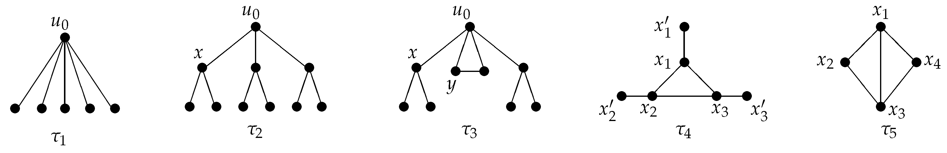
From [1], if is a decomposition of a graph G, then for arbitrary , that is to say are edge-disjoint in G. In this article, for graph G and an integer , if and there are at least two subgraphs such that are edge-joint, then is also called a decomposition of G, also denoted by . For example, is an edge-joint decomposition of , each of which is (see in Figure 1). Let be a path with n vertices, such that for , and are adjacent vertices in . By [9], is k-cutwidth critical, so we let for each . For G and which are homeomorphic, when no confusion occurs, if G is k-cutwidth critical after the series reductions are carried out, then we shall say that is also k-cutwidth critical. The following is immediate from Lemma 1:
Definition 1.
- (i)
- For graph G and integer , let with . For , define to be the component of that contains v.
- (ii)
- Let be two disjoint graphs with and . To identify u and v, denoted as , is to replace by a single vertex z incident to all the edges which were incident to u and v, where z is called the identified vertex.
- (iii)
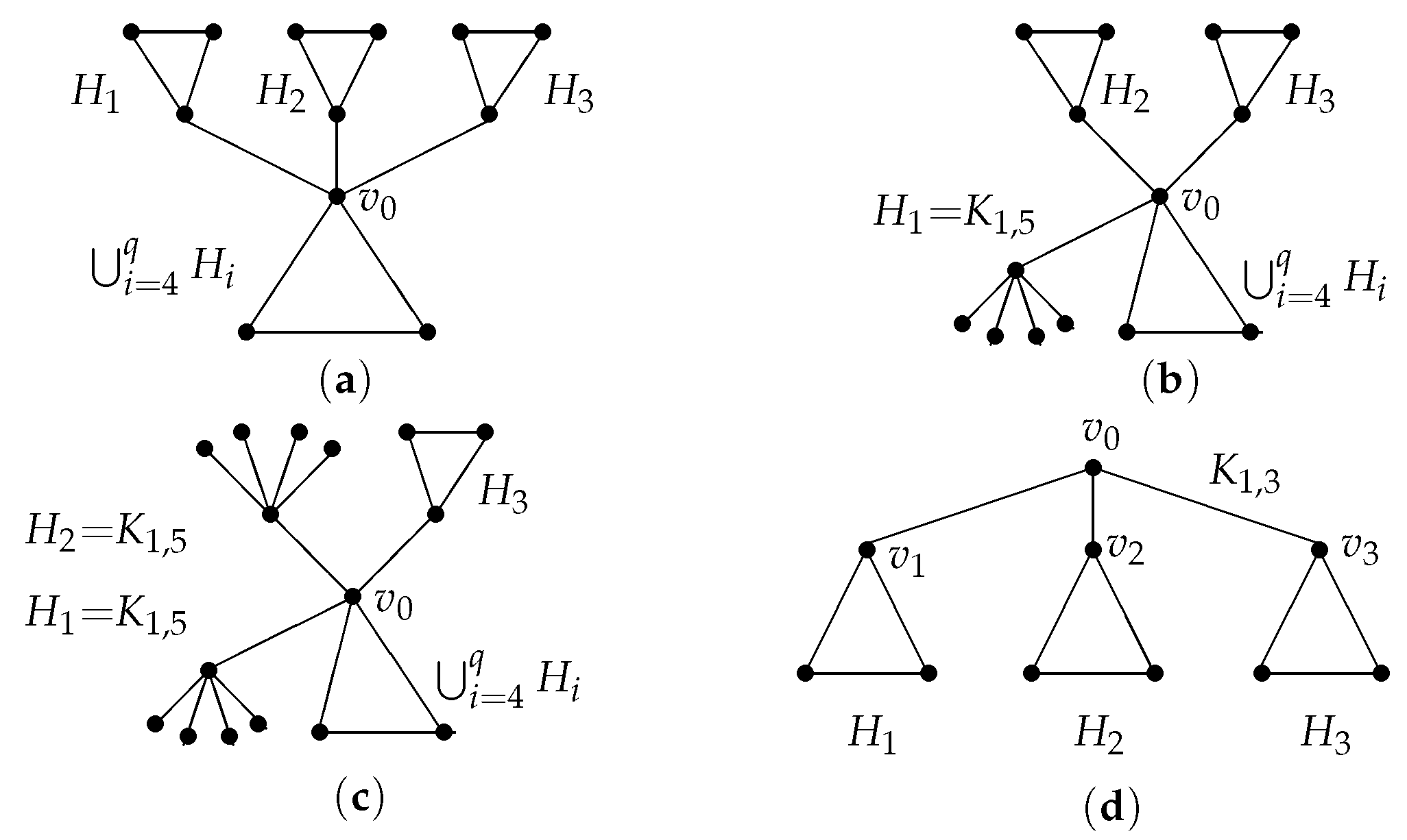
- Let , and be three disjoint graphs, and , for each . Define as the graph obtained from the disjoint union and by identifying with (again denoted as ) for each (see Figure 3d in Section 3.1 below).
- (iv)
- Let , and be three disjoint graphs, with and for each . Define as the graph obtained from the disjoint union and by identifying with (again denoted as ) for each .
- (v)
- For with , let be a graph with and . Define to be a graph obtained from disjoint union of by identifying into a single vertex in G. As in , is viewed as the vertex in .
- (vi)
- If , then define to be the family of all proper maximal subgraphs of G.
Definition 2.
Suppose that vertex with , are two cut edges of G, , and . For , let be an optimal labeling of , and let the labeling of G be as follows: for ,
Then, the labeling π is called a labeling by the order or ,.
Theorem 1
([12]). For any , if there always are two vertices in such that are cut edges in G, then if and only if
Corollary 1.
For graph G, if there is a vertex such that holds for any , then k, where are both cut edges in G.
Lemma 5
([10]). Let graph G be k-cutwidth critical and . Then for .
Theorem 2
([12]). With the notation of Definition 1, let at least one of , say , be -cutwidth critical with . Then .
Corollary 2
([12]). With the notation of Definition 1, for each , if is -cutwidth critical with , then is k-cutwidth critical.
Theorem 3.
With notation of Definition 1, if for each , then .
Proof.
Let . If for or 3 then the series reductions are first carried out without effecting . As has three components and with cutwidth , similar to that of (5), an optimal labeling obtained by the order satisfies . Therefore, by (2). Additionally, it is not hard to verify that by Corollary 1; this is because for any . Hence , i.e., . □
Corollary 3.
With notation of Definition 1 (iv), if the following hold:
- (1)
- are 2-connected;
- (2)
- is a small-cut vertex corresponding to an optimal labeling of for each ;
- (3)
- , are -cutwidth critical, then is k-cutwidth critical, where are not necessarily distinct.
Proof.
Let . Since , and . First, by Theorem 3. Second, we show for any , that is, G is k-cutwidth critical. Because any can be obtained by deleting a pendant edge or an non-pendant edge in G, , where is a cycle with length . There are two cases to consider: (1) ; (2) or . For Case (1), since is -cutwidth critical, there is an optimal labeling such that . Now, by Lemma 5, let be a labeling of such that for . Thus, a labeling of G by the order is obtained with implying . For Case (2), let . By assumption, . Since is a small-cut vertex corresponding to an optimal labeling of for each , a labeling of G by the order is obtained with implying . Likewise, if then also. To sum up, G is k-cutwidth critical. □
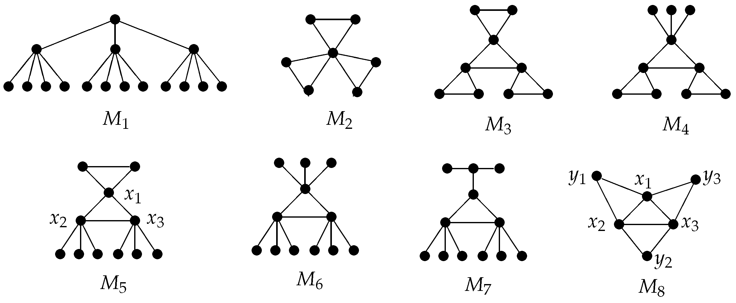
Lemma 6.
Each graph in Figure 2 is 4-cutwidth critical.
Figure 2.
Eight special 4-cutwidth critical graphs.

Proof.
Two steps can be used to finish the proof. For each , Step 1 is used to show . This can be accomplished by two operations: for any labeling of , which implies ; has an optimal labeling with . In Step 2, for any , must be shown. Since operation of each of the two steps is easy, we omitted it here.
Let v be a cut-vertex with in G and be q connected components of . Then, , denoted by , is called the ith v-component of . A vertex is called the central vertex of a k-cutwidth graph G if is a cut-vertex in G, such that all -components of can form a decomposition of G in which each element has equal cutwidth with . For example, for graph in Figure 1, with edge is the ith -component of ; we can see that is a decomposition of , each of which is a 2-cutwidth critical tree , so is the central vertex of . Likewise, each of has a decomposition of equal cutwidth-2 and a central vertex also, respectively.
For a cycle of G with and for , let be a vertex-cut set of G. If is also an edge-cut set of G and is the ith connected component of leading from , then , denoted by , is called the ith -component leading from of , where and at least an . A cycle with is called a central cycle of a k-cutwidth graph G if is an edge-cut set, such that one of the following is a decomposition of G, each element of which has equal cutwidth with ,
- (1)
- , or
- (2)
- in which may be one of with , and there exists at least , or
- (3)
- , each of which is either or with , and there exists at least , where and .
For example, in Figure 1, has a cycle , and has three components , each of which equals . Let and , and let for . Then, is a decomposition of , in which each member is a 2-cutwidth critical subgraph , and is the central cycle in . For Case , we take with a central cycle in Figure 2 as an example. also has three connected components , which are and three -components with , with and , respectively. Let , then and is a decomposition of equal cutwidth 3 of , each member of which is also 3-cutwidth critical.
In the case that G is 2-connected and is not an edge-cut set of G, suppose that has q connected components , with for each , and let be the ith 2-connected subgraph that contains edge . If is a subgraph decomposition of equal cutwidth , then is also called the central cycle of G. For example, let with in Figure 2. Clearly, has three components , and is an edge-joint subgraph decomposition of equal cutwidth 3 of G. Hence, is the central cycle of . □
From Lemma 2, we have
Theorem 4.
For a 2-cutwidth critical graph , one of the following holds:
- (1)
- G has a central vertex , and -components of constitute a decomposition with , each of which is with cutwidth 1;
- (2)
- G is a cycle , whose three edges constitute a decomposition with , each element of which is with cutwidth 1.
Theorem 5.
For a 3-cutwidth critical graph , one of the following holds:
- (1)
- has a central vertex , and -components of constitute a decomposition with , each of which equals or with cutwidth 2; or
- (2)
- G has a central cycle with = 3 for , and -components of constitute a decomposition with , each member of which equals with cutwidth 2; or
- (3)
- G equals or , where is a cycle of length 4.
3. 4-Cutwidth Critical Graphs with a Central Vertex
In this section, we shall verify the decomposability of the 4-cutwidth critical graphs with a central vertex. Since a k-cutwidth critical graph G is homeomorphically minimal, for the central cycle of G, we can let
3.1. 4-Cutwidth Critical Trees with a Central Vertex
Definition 3.
For a cut-vertex with in a tree T, let be a -component of with and , then define
If for , then is called a subtree decomposition of equal cutwidth of T.
In Definition 3, for a decomposition of equal cutwidth of a k-cutwidth critical tree T, (). If , then is edge-joint; Otherwise is edge-disjoint.
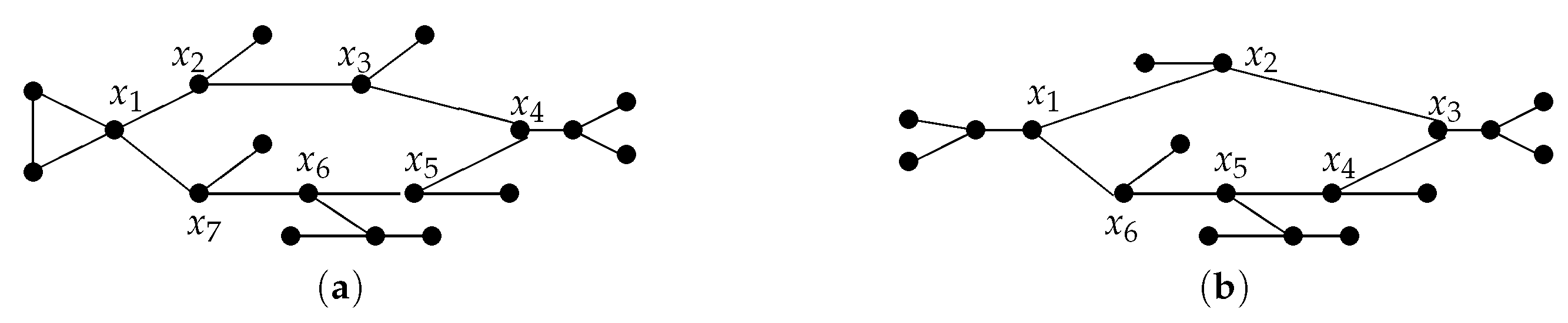
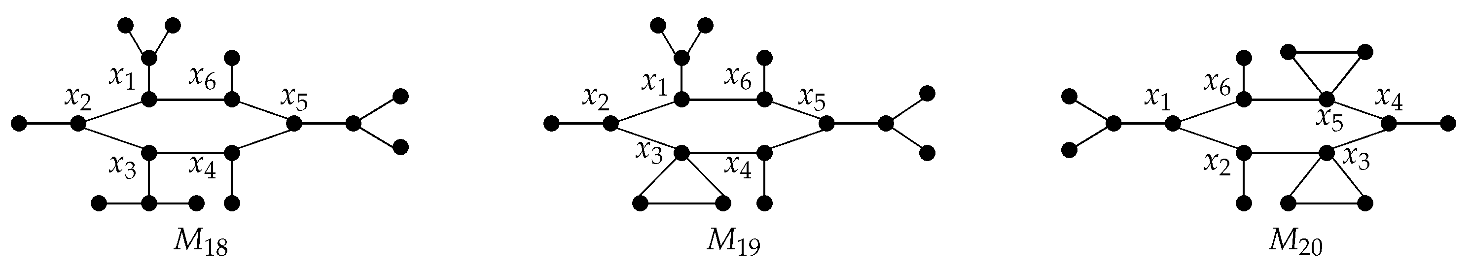
There are eighteen 4-cutwidth critical trees in total by [9], each of which can be decomposed into three 3-cutwidth subtrees by Lemma 3. In fact, among these eighteen 4-cutwidth critical trees, each possesses one of the structures listed in Figure 3, in which is either one of and or homeomorphic to for in Figure 3a. is either or homeomorphic to for in Figure 3b, is either or homeomorphic to for in Figure 3c, either or with is in for in Figure 3d. Thus, based on this, (see Figure 2) is 4-cutwidth critical, and again we have the following:
Theorem 6.
For a 4-cutwidth critical tree T, one of the following holds:
- (1)
- T possesses a configuration which can be decomposed into three edge-disjoint 3-cutwidth trees and (not necessarily distinct), and the 3-degree vertex of is the central vertex of T, where is a -component of with either or for each (see Figure 3d); or
- (2)
- T is a tree with a central vertex with and with an edge-joint decomposition of equal cutwidth 3, where and (not necessarily distinct), which are defined by (7), are either in or homeomorphic to , and at least one of them, say , is not (see Figure 3a–c, respectively).
Figure 3.
Four structures of 4-cutwidth critical trees.

3.2. 4-Cutwidth Critical Nontrees with a Central Vertex
We shall focus primarily on the structures of 4-cutwidth critical non-trees with a central vertex in this subsection.
Suppose now that and (not necessarily distinct) are mutually disjoint graphs, and at least one of them is not a tree. Let be a graph obtained from the disjoint graphs and by identifying with (again denoted as ) for , where
is a pendant vertex of and for . Obviously, if and then is the central vertex of .
Lemma 7.
Suppose that is -cutwidth critical for , then is a k-cutwidt critical graph, where are not necessarily distinct.
Proof.
Let . If there exists at least a vertex such that , then the series reductions can be implemented first. Two cases need to be considered as follows.
Case 1. For , .
By , for . So by assumption, and by Lemma 5. Now, let be the labelings such that and , respectively. Then, a labeling of G by the order is obtained, and , implying . Since and are cut-edges in G, for any , leading to by Corollary 1. Hence .
On the other hand, any can be obtained by deleting a vertex y with degree one of a pendant edge or a nonpendant edge in G, so or , where is a cycle with length in G. Without loss of generality, let . If is pendant with , then by the criticality of , with a labeling such that . Since and are -cutwidth critical, by in Lemma 5, two labelings can be obtained such that with and with , respectively. Now, define to be a labeling of by the order , then , i.e., , meaning that G is k-cutwidth critical. Likewise, if is not pendant with , then , and a labeling by the order is also obtained, under which , i.e., , meaning that G is also k-cutwidth critical. The cases of or are the same as that of , omitted here.
Case 2. There are at least a , such that .
Three subcases need to be considered: there is unique (say ), such that ; there are two (say ), such that and ; for each . For Subcase , since , with . In this case, , i.e., , and by . Similarly, for Subcase , , and ; for Subcase , , and . The remaining argument of any Subcase is similar to that of Case 1, omitted here. To sum up, G is k-cutwidth critical. □
Corollary 4.
Suppose that for , then is a 4-cutwidt critical graph, where at least a , and are not necessarily distinct.
Corollary 5.
Suppose that for , then is a 4-cutwidt critical graph, where at least a , and are not necessarily distinct.
Lemma 8.
Let , be 3-cutwidth critical with for and satisfy the following:
- (i)
- each non cut-edge of may be subdivided once, and may possibly be the subdivision vertex;
- (ii)
- ;
- (iii)
- if , then is not either the central vertex or the pendant vertex of it;
- (iv)
- for or 3 if .
Then, is a 4-cutwidt critical graph, where are not necessarily distinct, and at least one of them is not in .
Proof.
Let . By assumption, for , with or with and . So, or for and for . Thus, with an argument similar to that of Lemma 7, G is 4-cutwidth critical. □
Suppose that with the central vertex (=) and two cut edge , such that any -component of is 2-cutwidth critical (see in Figure 1). For any 3-cutwidth nontree graph with cycle , if there is a vertex (say ) in such that when with the central vertex (=); or if is a component of leading from , then either with when or only when ; or and are not necessarily distinct; or if and , then . Only then, by , do we have
Lemma 9.
Graph is a 4-cutwidth critical graph.
Proof.
Let with optimal labeling , and be a sublabeling of restricted on . By assumption, has three -components and , each of which is either or by Theorem 3. Suppose that is obtained by the order with for if are optimal labelings of and , respectively. Without loss of generality, let with cutwidth 2. Since is 3-cuwidth critical and in , whether or with , if is a -max-cut of G, then and . Hence, . On the other hand, assuming that are cut edges in G, when or when , so , resulting in by Corollary 1. Thus, .
We now verify that G is 4-cutwidth critical. For any edge , e is in either or . Since which is 3-cutwidth critical, if then we can always find a labeling of such that and . For , we can always find an optimal labeling of such that . Thus, a labeling of by the order is obtained with leading to . Similarly, if then also. This completes the proof. □
From Lemma 9, we can see that if a critical non-tree G with cutwidth 4 can be decomposed into two 3-cutwidth critical subgraphs and , then G has a central vertex ; is also the central vertex of at least one of and . For example, let with a pendant vertex be the copy of with a pendant vertex y, and be the copy of y, be a vertex of a 3-cycle . Then, graph , obtained by identifying into a vertex , is a 4-cutwidth critical graph with the central vertex , and this graph can be decomposed into two 3-cutwidth critical subgraphs with the central vertex , and with the central vertex ; there are at least two cut edges .
Lemma 10.
Let G be a 4-cutwidth critical nontree graph with the central vertex and at least two cut edges and . If G can be decomposed into two 3-cutwidth graphs (not necessarily distinct), then the following hold:
- (1)
- are in ;
- (2)
- at least one of and , say , is in , while ;
- (3)
- is the central vertex of , but is only a vertex of any 3-cycle of .
Proof.
Since G is a non-tree graph, we do not consider the cases that and are both or . We first show that are in by contradiction. Suppose that there is some (say ) such that but is not 3-cutwidth critical, then there is at least a pendant edge with or a non-pendant edge such that or , respectively, where is a cycle with length . For the former, because by assumption, by Lemma 9. Likewise, for the latter, also by Lemma 9. All are contrary to the criticality of G. Hence are both in .
Next, by the assumption that is the central vertex and and are both cut edges in G, we claim that at least one of and (say ) must be or . This is because otherwise, there is at most a vertex such that is a cut edge in G if and are both in , which is a contradiction. So holds and .
Third, assume that is neither the central vertex of nor a vertex of a 3-cycle of if . Without loss of generality, let . Then is either or one of . For , by assumption, is not also the central vertex of . Thus, except three vertices of 3-cycle of , three cases need to be considered: is not only a subdivision vertex of some non-pendant edge in but also a subdivision vertex of some non-pendant cut edge in ; is a subdivision vertex of some non-pendant edge in , but is a nonpendent vertex of ; is not only a non-pendant vertex of but also a non-pendant vertex of . For any case of Cases –, we can easily verify that by Lemma 1(3) and Theorem 5, contrary to the assumption of . Likewise, for , there are only two cases to consider: is a subdivision vertex of some non-pendant edge in , but is a arbitrary vertex of ; is a nonpendant vertex of , but is a arbitrary vertex of . Furthermore, in any case, , also a contradiction. This completes the proof. □
For a cut-vertex graph G and all -components of , we define a decomposition each of which has cutwidth 3 below. Let be an edge subset taken from such that the cutwidth of the connected subgraph is 3 if , for . Then, we obtain the following:
Definition 4.
For a cut-vertex of G and the -component of , and the cutwidth of is three. For , define
If for , then is called a decomposition of equal cutwidth 3 of G, and G is called a graph with a central vertex , where is an edge subset taken from such that if for
Lemma 11.
Let G be a 4-cutwidth critical graph with the central vertex and at least two cut edges and . If G can be decomposed into three 3-cutwidth graphs and , then G is 4-cutwidth critical if and only if each of is either a 3-cutwidth critical graph or homeomorphic to a 3-cutwidth critical nontree graph, and is not the central vertex of if .
Proof.
The proof is straightforward using Lemma 4, omitted here. □
Lemma 12.
For a 4-cutwidth graph G with a central vertex , if has at least three -component and each is 2-connected in G, then G is 4-cutwidth critical if and only if (see in Figure 2).
Proof.
Sufficiency: this is obvious using Lemma 6.
Necessity: By assumption, for any vertex , , where is a cycle of and for any only. Since is a minor of any and , with cutwidth 4 is a minor. Hence by the criticality of G. □
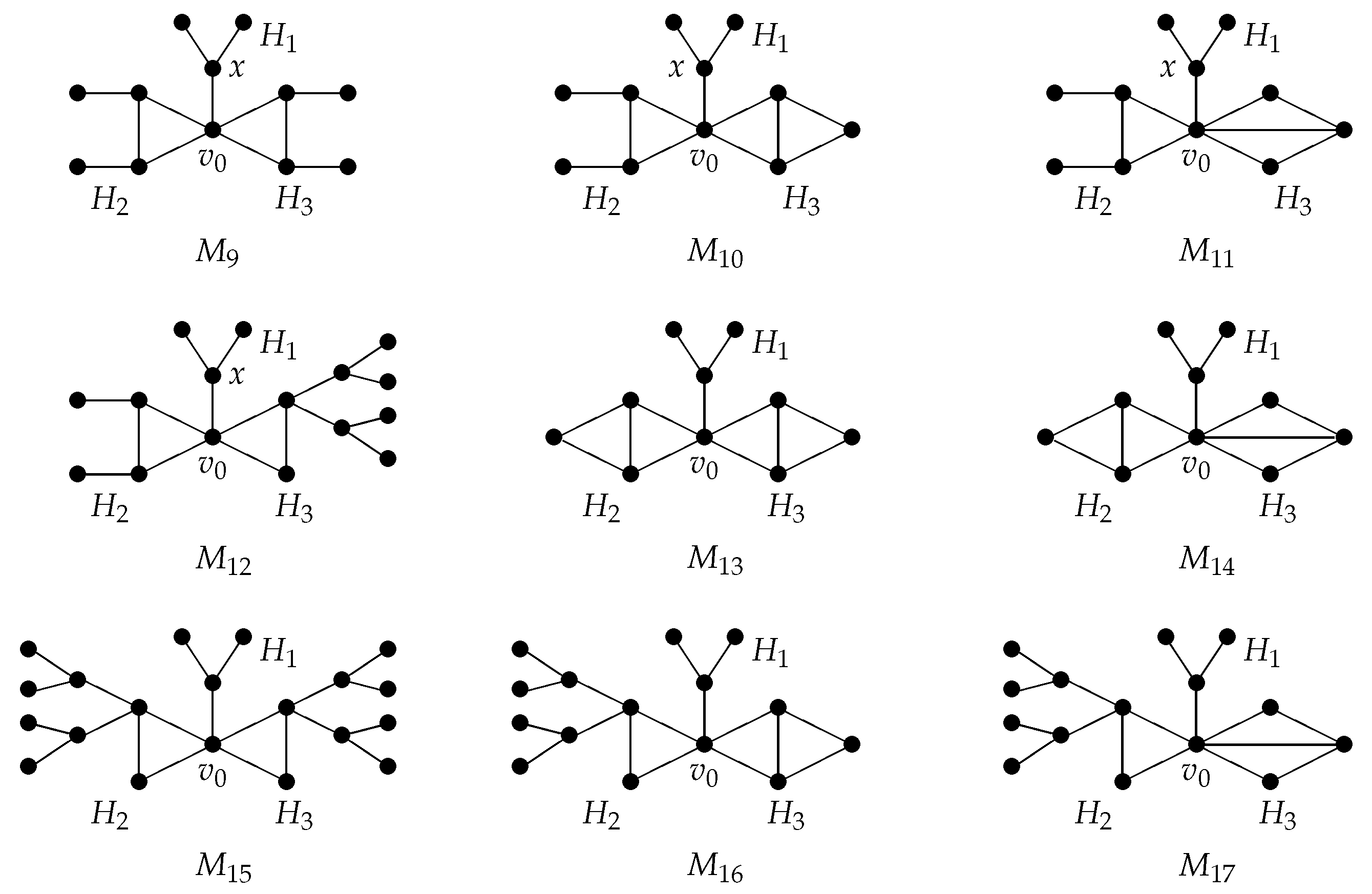
Lemma 13.
Proof.
Similar to that of Lemma 6, we can show that graphs – in Figure 4 are all 4-cutwidth critical.
Sufficiency: For graph , let , and , is the subgraph decomposition desired. Likewise, for graphs –, let , , with and or 3, respectively; for graphs –, let , with , with and or 3, respectively, is the subgraph decomposition desired.
Necessity: Suppose by contradiction that . By assumption, for , and for . Three cases, which are at least a for , and with , respectively, can be first excluded; this is because that G either is a tree or is not 4-cutwidth critical in these cases, which is a contradiction. Thus, noting that 3-cutwidth critical subgraphs , are symmetrical in G and is sufficient to verify two cases:
- (1)
- , one of whose three pendant vertices is , and ;
- (2)
- , one of whose three 2-degree vertices is , and .
By assumption, we do not consider the following five subcases contained in cases (1) and (2), respectively:
- (a1)
- because of ;
- (a2)
- is a subgraph of G because of ;
- (a3)
- G is a tree because G is a non-tree graph;
- (a4)
- is a decomposition of equal cutwidth 3;
- (a5)
- because G is 4-cutwidth critical.
Based on this, for cases (1) and (2), we only consider vertices , x of , vertices of , vertex of and vertices of (see Figure 1), respectively, which may be the central of G. For convenience, let , , where are copies of corresponding to of , are copies of corresponding to of ; is a copy of corresponding to of , and and are copies of corresponding to of , respectively. In this case, we can see that there are at least a , which is a decomposition of one of not considered here. For example, is a decomposition of . So, by at most direct operations and at most computations without considering by assumption, we can see that G is not 4-cutwidth critical, which is a contradiction. Hence, . □
From Lemmas 7–13, we have:
Theorem 7.
For a 4-cutwidth non-tree graph G with a central vertex , G is 4-cutwidth critical if and only if G has one of the following six configurations.
- (1)
- For , if is some in Figure 1 and corresponding to is a graph defined in , then , where and are not necessarily different;
- (2)
- , where with for and corresponding to is a graph defined in , for and for is not either the central vertex or the pendent vertex when but is possible to a subdivision vertex of a non cut-edge of when ;
- (3)
- with the central vertex of , where with the central vertex of or , respectively, see Figure 1 with a 3-cycle and with , corresponding to is a graph defined in ;
- (4)
- G has a subgraph decomposition of equal cutwidth 3, defined in Definition 4, where G is a graph with a central vertex of and at least two cut edges , is 3-cutwidth critical for ;
- (5)
- G has a subgraph decomposition of equal cutwidth 2, each of which is a -component of , where is the central vertex of degree 6 of G, and and are the copies of a 3-cycle ;
- (6)
- G is one member of with a central vertex (see Figure 4) and a subgraph decomposition , in which , one of whose pendant vertices is , for , where satisfies:
- (i)
- is a 2-degree vertex y of of for ;
- (ii)
- if the 3-degree vertex of is x and , then and is a 3-degree vertex of ;
- (iii)
- is either a 2-degree vertex of or a 3-degree vertex of for , but if and is a 3-degree vertex of , then must not be a 3-degree vertex of , and vice versa.
4. 4-Cutwidth Critical Graphs with a Central Cycle
In this section, we aim to investigate 4-cutwidth critical graphs with a central cycle with .
Lemma 14.
Assume that graph G is 4-cutwidth critical with a central cycle of length q, then .
Proof.
Assume, contrary to that, that and is the ith connected component leading from of . Without loss of generality, let , i.e., with for (see an example in Figure 5a), and let be an optimal 4-cutwidth labeling with . By the criticality of G, we may always assume that . By direct computations, there are at least three s (say and ) such that and . Otherwise, , contrary to . Since G is 4-cutwidth critical, we can let , say and (see Figure 5a). In this case, and for any with , contrary to the criticality of G. On the other hand, there is at least a 4-cutwidth critical graph G with a central cycle such that , and for (see Figure 5b). Hence . □
From Lemma 14, in the sequel, we shall characterize the 4-cutwidth critical graphs with a central cycle of lengths 3–6, respectively.
4.1. Graphs with a Central Cycle of Length Three
Definition 5.
Let be the central cycle of G, be the ith connected component leading from of , and be cut vertices in G. Then, for , define
If, for each , with or 3, then is called a decomposition of equal cutwidth ρ of G; if there are at least two (say ) such that and , then is called a decomposition of nonequal cutwidth ρ with or 3 of G, where and are not necessarily distinct, and is not necessarily non-empty.
Lemma 15.
With notation in Definition 5, let G be 4-cutwidth critical with the central cycle , be cut vertices in G, and has at least two vertices (say ) such that and . If is a decomposition of nonequal cutwidth ρ with or 3, then is ρ-cutwidth critical for except in Figure 2.
Proof.
Since is a decomposition of nonequal cutwidth with or 3, we can assume that , but , implying . Since G is 4-cutwidth critical with and , or , or for by Lemma 6, meaning to that or for . Thus, for and , there are three cases to consider: (i) , ; (ii) , ; (iii) , , where are the central vertices of and , respectively (see in Figure 2 and Figure 6d,e below). In any of Cases (i)–(iii), with or with . Thus, we can see that is 2-cutwidth critical for and 3-cutwidth critical for . Now let but with and ; then, we can conclude that by the 4-cutwidth criticality of G, which has a decomposition of equal cutwidth two in which and are the copies of . This is because in this case, if is a decomposition of nonequal cutwidth of 2 and 3 of G, then edge . As for each in this case, this decomposition of nonequal cutwidth does not hold. Thus, this case is not possible. The proof is complete. □
Lemma 16.
With notation in Definition 5, let be a decomposition of nonequal cutwidth ρ with or 3 of 4-cutwidth graph G with the central cycle . If is ρ-cutwidth critical for , then G is 4-cutwidth critical, where are all cut vertices, and has at least two vertices (say ) such that and .
Proof.
Let be an optimal labeling of G with and intervals with , respectively. Then, is embedded in with congestion 3, is embedded in with congestion 4, is embedded in with congestion 3. Herein, and are a star with center or two stars with an identifying leaf at . Let denote combining with the two edges in incident with . Then for . As for embedded in with congestion 4, since the central cycle yields congestion 2 in , we chose as a 2-cutwidth critical tree, namely, a , such that either or . For this construction, the maximum congestion is 4, i.e., . Furthermore, for any edge , if , then the deletion of e reduces the congestion 2 of cycle-edge in by one. Hence embedded in has congestion 3, and so . If , for Case (i) in Proof of Lemma 15, two subcases need to be considered: with for each ; with for , but with for . Without loss of generality, we can let with . Since with congestion 1, we can embed in , in and in , respectively, which results in . So does the case of (or ). Likewise, for Cases (ii) and (iii) in Proof of Lemma 15, for any also. Therefore, G is 4-cutwidth critical. The lemma holds. □
Lemma 17.
With notation in Definition 5, let G be 4-cutwidth critical with the central cycle , where are all cut vertices in G, and has at most one vertex (say such that . If is a decomposition of equal cutwidth 3, then ( or with is 3-cutwidth critical for .
Proof.
We first give Claim 1 below.
Claim 1. There is at least such that is one of and (say ) with , where and .
Let or with for each . As the arguments are similar, we only consider two cases: (a) with , with for ; (b) with for each . For Case (a), is a pendent edge of for , and . So, also and by a series reduction in and , respectively. Thus, which results in that by Theorem 3, contrary to the criticality of G. For Case (b), and for each , so every by a series reduction in and . Thus, there is an edge in , say , such that . Hence by Theorem 2, also a contradiction. Claim 1 holds.
From Claim 1 and assumption, there are nine cases to consider, as follows (see graphs – in Figure 6 below):
- (1)
- with , and ;
- (2)
- with , and ;
- (3)
- with , and ;
- (4)
- with , and ;
- (5)
- with , and ;
- (6)
- with , and ;
- (7)
- , and ;
- (8)
- , and ;
- (9)
- , and ,
where for in Cases –, and for each in Cases –. We consider Case by contradiction. Assuming that there is at least an edge such that , i.e., is not 3-cutwidth critical. There are three subcases to consider: with ; with ; with . For Subcase , by assumption and Definition 3, for , , is 3-cutwidth critical, and , so either or . Thus, if (say ), then is changed to with cutwidth 4 resulting in ; if , i.e., then is changed to be with cutwidth 4 resulting in . So by again, and contrary to that, G is 4-cutwidth critical. For Subcase , we can conclude that and either or with cutwidth 3. By Lemma 1(3), an optimal labeling by the order of can be obtained, and , implying . So, by the optimality of , also a contradiction. The argument of Subcase is the same as that of Subcase , omitted here. Thus, for Case , is 3-cutwidth critical for . Similarly, for Cases –, is also 3-cutwidth critical for . This completes the proof. □
Lemma 18.
With notation in Definition 5, let be a decomposition of equal cutwidth 3 of graph G with the central cycle , where are all cut vertices of G, and has at most one vertex (say such that , and either or . If is 3-cutwidth critical or there are at least a with for , then G is 4-cutwidth critical.
Proof.
By Lemmas 1, we can show . By assumption again, and . There are nine cases – listed in Proof of Lemma 17 to consider. For each case , via using an argument similar to that of Lemma 16, we can show for any , omitted here. □
Lemma 19.
Let G be a 2-connected graph with a central cycle . Then G is 4-cutwidth critical with a decomposition of equal cutwidth 3 if and only if (see Figure 2).
Proof.
Sufficiency. Since , G is 4-cutwidth critical by Lemma 6. Clearly, let for , then is a decomposition desired because of for each .
Necessity. In fact, since G is 2-connected with a central cycle and a decomposition of equal cutwidth 3, the arbitrary two vertices and of must be in a cycle and , where . That is to say, by the criticality of G, there must be another vertex in G such that and for each . In this case, , induced by . Hence . □
Lemma 20.
Assume that G is a 4-cutwidth critical graph with a central cycle , then G has an edge-disjoint decomposition of equal cutwidth 2 if and only if (see Figure 2), where is a cut vertex and is the connected component of leading from for .
Proof.
Sufficiency is obvious in Lemma 6, omitted here.
Necessity: Let be an optimal labeling of G with and . Then, the number set is divided into three intervals and and are embedded into in different manners, respectively. As are all 2-cutwidth graphs and is a cut vertex in G for , is embedded into with congestion 2, is embedded into with congestion 4, and is embedded into with congestion 2. By the criticality of G and , is either a star with the 3-degree vertex or a cycle , which is a copy of for . As for embedded in with a congestion of 4, the central cycle leads to a congestion of 2 in , so must be either a or a copy of such that or 5. Thus, G must be one member of , each element of which has a edge-disjoint decomposition of equal cutwidth 2, where is either or for . □
Theorem 8.
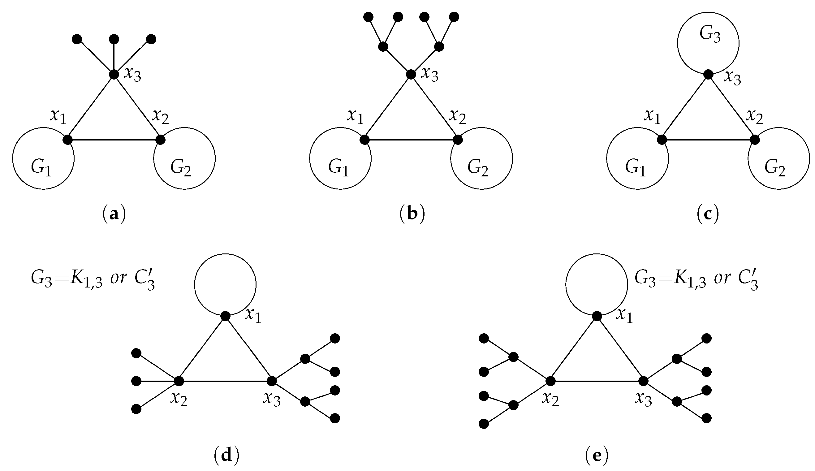
For a 4-cutwidth nontree graph G with a central cycle , G is 4-cutwidth critical if and only if G has one of the following configurations.
- (1)
- (2)
- G has a decomposition of equal cutwidth 3 in which or with is 3-cutwidth critical, and at least a (say ) contains at least two edges and of , where is a cut vertex for each and there is at most a vertex (say ) such that (see Illustration in Figure 6a–c);
- (3)
- G is 2-connected and (see Figure 2) with a decomposition of equal cutwidth 3 in which for ;
- (4)
- with an edge-disjoint decomposition of equal cutwidth 2, in which is either or a copy of for (see – in Figure 2).
Figure 6.
Illustrations of Theorem 8.

4.2. Graphs with a Central Cycle of Length Four
For a graph G with a central cycle with length 4, suppose that is the ith connected component leading from of , and , and has no , such that but for any proper subgraph . Let when or with and when , and for with , where are all cut vertices in G, and there is at least a vertex between and (say ) such that . Then, we have the following:
Lemma 21.
For a graph G with the central cycle , if is a decomposition of equal cutwidth 3 of G and is 3-cutwidth critical for each , then G is 4-cutwidth critical (see Illustrations in Figure 7).
Proof.
By assumption, , and since is 3-cutwidth critical for , , with and with or with resulting in . Suppose that is a labeling of G with , then is partitioned into three intervals and . Now, we embed in with congestion 3, in and connect with congestion 4, in with congestion 2. Thus, , implying . On the other hand, . Hence .
The remaining is to show for any . There are three cases to consider: ; ; e is a pendant edge of for . For Case , . Since , by Lemma 1(3), if is a pendant edge of with , then we can find an optimal labeling with , under which is embedded in interval with congestion 3. If (note that or in this subcase), then we can find an optimal labeling with , under which is embedded in interval with congestion 3. So . Similarly, for Cases and , also. Hence, G is 4-cutwidth critical. □
Lemma 22.
Let G be a 4-cutwidth critical graph with the central cycle . If G has a decomposition of equal cutwidth 3, then is 3-cutwidth critical for each (see Illustrations in Figure 7).
Proof.
By contradiction, suppose that there is at least a (say ) such that is not 3-cutwidth critical, then there exists an edge such that also. Two cases need to be considered: is a pendant edge with in ; if contains a cycle which does not equal the central cycle . Using an argument similar to that of Lemma 21, for Case , we can find a labeling with , thereby contradicting that G is 4-cutwidth critical. Furthermore, likewise, for Case , we can find a labeling with , also contradicting that G is 4-cutwidth critical. Similarly, if for or 4 then we can also find a contradiction to the assertion that G is 4-cutwidth critical. Therefore, is 3-cutwidth critical for each . □
From Lemmas 21 and 22, the structure of a 4-cutwidth critical graph G with a central cycle can be obtained below.
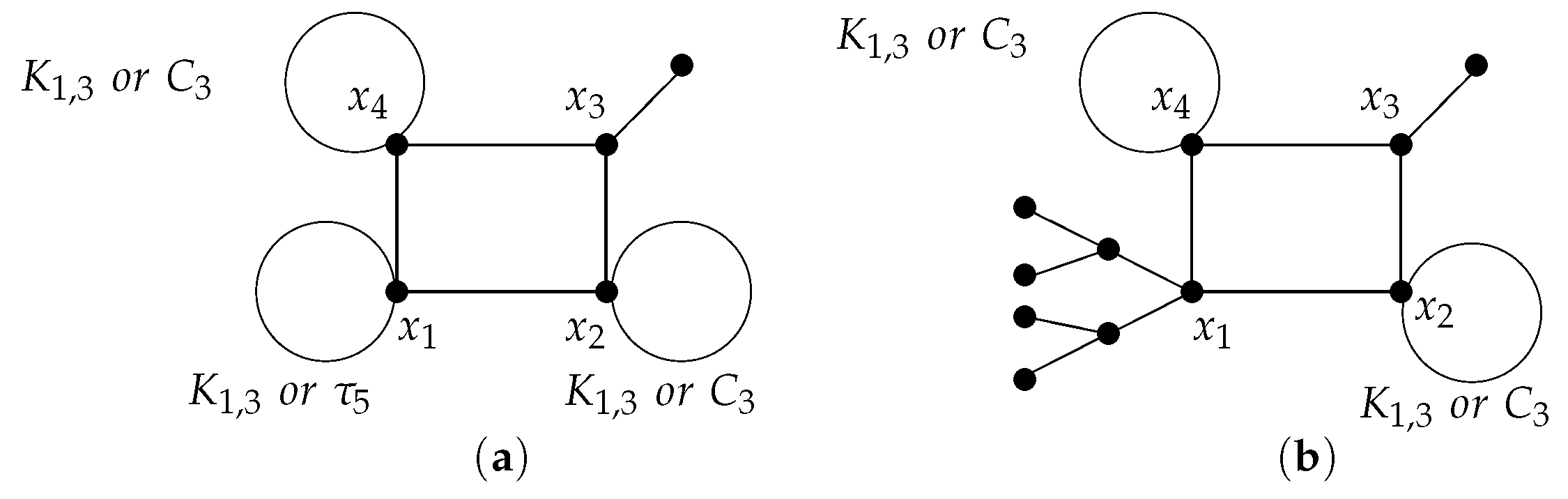
Theorem 9.
Assume that G is a 4-cutwidth graph with a central cycle , and is a cut vertex for , then G is 4-cutwidth critical if and only if G has a decomposition of equal cutwidth 3, each of which is 3-cutwidth critical, where are one of the following:
Figure 7.
Illustrations of Theorem 9.

4.3. Graphs with a Central Cycle of Length at Least Five
Suppose that G is a graph with the central cycle , and for , has no component leading from , such that , but for any proper subgraph , has at most two with , where . Let one of the following hold:
- (1)
- , or if or if for with ;
- (2)
- , , with and , for ;
- (3)
- is homeomorphic to subgraph , , with , where has at most two 4-degree vertices (say, and ) which are nonadjacent.
Then, we have the following:
Lemma 23.
For a graph G with the central cycle , if G is 4-cutwidth critical and is a subgraph decomposition of equal cutwidth 3 of G, then (or is 3-cutwidth critical for (see Illustrations in Figure 8).
Proof.
By contradiction, we first consider Case above. Suppose that there exists some , say first, such that is not 3-cutwidth critical. There are two subcases to consider: (i) contains no cycle; (ii) contains at least a cycle. For (i), has at least a pendant vertex v such that . By , let be cut edges in G with and . Then , and are both cut edges in clearly. So, by Lemma 1(3), has an optimal labeling such that the vertices in each of , and are labeled consecutively. Without loss of generality, let and . Then . Since is optimal, , contradicting that G is 4-cutwidth critical. For (ii), two subcases need to be considered: (a) has at least a pendant vertex v such that ; (b) has at least a non-pendant edge e such that . Subcase (a) is the same as case (i), omitted here; For subcase (b), using a similar method to that of case (i), we can show , also a contradiction. Now, we consider or , and without loss of generality; let with and . Assume that there is an edge e such that , i.e., is not 3-cutwidth critical. Similar to Case (i), , and are both cut edges in . By Lemma 1(3), has an optimal labeling such that the vertices in each of , and are labeled consecutively with and . Thus , contradicting that G is 4-cutwidth critical. Likewise, let and be one of the followings, and one of be not 3-cutwidth critical: (A1) each with for ;
(A2) each with for ;
(A3) with but , with ;
(A4) with , with but .
Then we can also obtain a contradiction to the assertion that G is 4-cutwidth critical. Hence, each (or is 3-cutwidth critical.
Similarly, for Cases and above, (or is also 3-cutwidth critical for . This completes the proof. □
Lemma 24.
For a 4-cutwidth graph G with the central cycle , if is a decomposition of equal cutwidth 3 of G, (or is 3-cutwidth critical for , then G is 4-cutwidth critical.
Proof.
Three cases similar to those of Lemma 23 need to be considered. We first consider Case by contradiction. Suppose that G is not 4-cutwidth critical, i.e., there exists a pendant vertex v (or a non-pendant edge e) such that (or ). There are three subcases to consider: (or ); (or ); (or ). For Case , by assumption, (or ). Since , using a similar method to that of Lemma 22, we can verify that (or ) contrary to (or ). So, G is 4-cutwidth critical. Likewise, for Subcases and , G is 4-cutwidth critical also.
Similarly, for Cases and , G is 4-cutwidth critical also. This proof is completed. □
From Lemmas 23 and 24:
Theorem 10.
Assume that G is a 4-cutwidth graph with a central cycle , and is a cut vertex for , then G is 4-cutwidth critical if and only if G has a decomposition (or , , of equal cutwidth 3, where are one of the following:
- (1)
- with the central vertex of degree three or four, for , (or is one of and satisfies: , is not the central vertex of when , and are the pendant edges of when is or (see Illustration in Figure 8a);
- (2)
- is homeomorphic to with the central vertex of degree three, for , is homeomorphic to or with , where are not necessarily different (see Illustration in Figure 8b);
- (3)
- is homeomorphic to with the central vertex of degree four, for , is homeomorphic to or with , but if , then and vice versa (see Illustration in Figure 8b).
Figure 8.
Illustrations of Theorem 10.

In Figure 8a, is either which is or or with or which is in for ; Additionally, if then can be 3-cycle simultaneously.
Lemma 25.
For a graph G with a central cycle , G is 4-cutwidth critical if and only if in Figure 9.
Proof.
Sufficiency. For any , G can be easily shown to be 4-cutwidth critical by proving two conclusions: (1) ; (2) for any , omitted here.
Necessity. Let G be a 4-cutwidth critical graph with the central cycle .
Observation. For any , has a decomposition of equal cutwidth 3, where or with for , and .
By observation, suppose by contradiction that , then two cases need to be considered as follows.
Case 1. G has a decomposition of equal cutwidth 3, but there is at least an element in , say , such that does not equal (or ). In this case, has at least a connected component leading from , say , such that (or ); this is because the connected component leading from in is (or in any of is . Without loss of generality, let be a minimum graph such that (or ), i.e., (or ). Then, by direct computations, and , but G is not 4-cutwidth critical. Similarly, if or in then G is not 4-cutwidth critical also. So this case is not possible.
Case 2. G has not a decomposition of equal cutwidth 3. In this case, there are at least an element in , say , such that is either at most 2 or at least 4, i.e., either or . Since G is 4-cutwidth critical, the subcase of is impossible. For the subcase of , we claim that must be a path with length 2 in which either or . By direct computations, we can easily show that , contrary to . Therefore, this case is also impossible. The proof is complete. □
By Lemma 25, we have
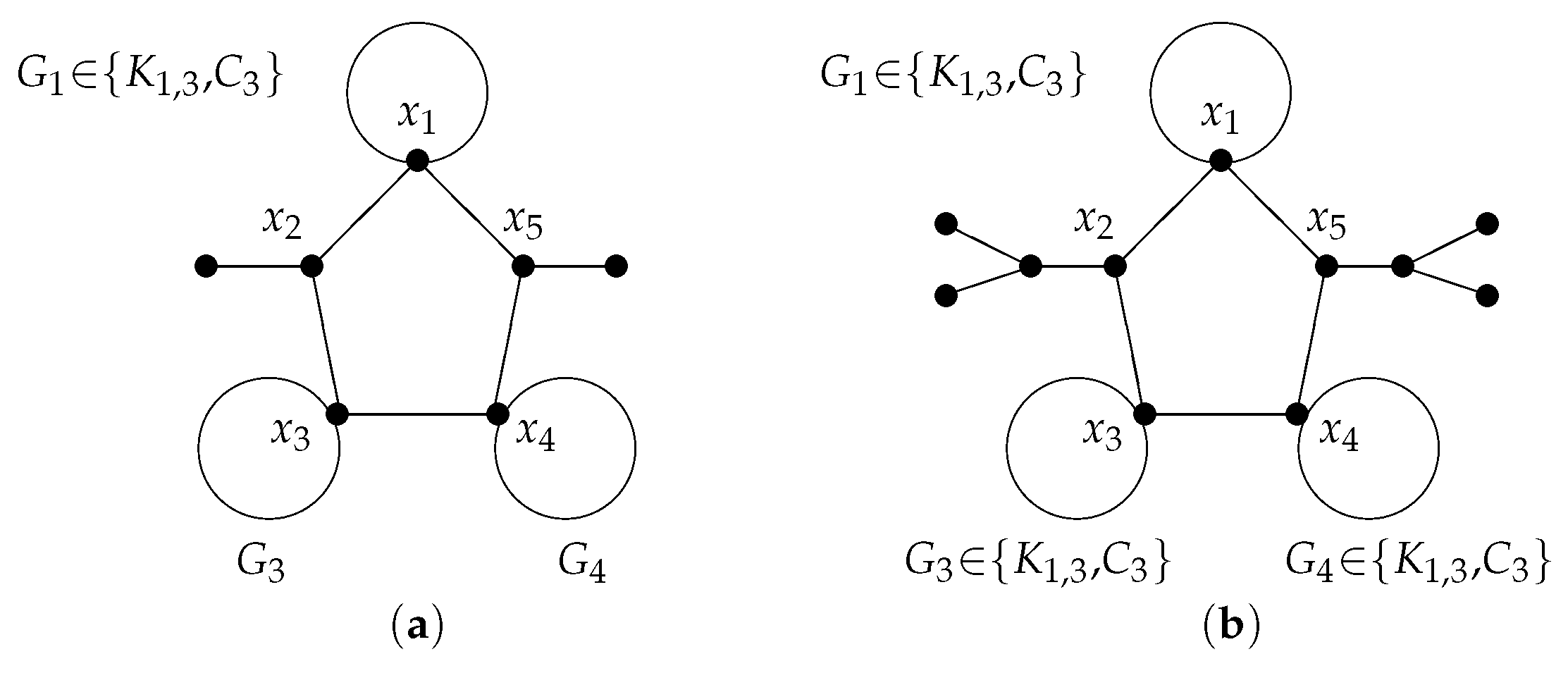
Theorem 11.
Let G be a 4-cutwidth graph with a central cycle . Then G is 4-cutwidth critical if and only if G is one of in Figure 9, which has a subgraph decomposition of equal cutwidth 3, in which or with central vertex for and there is at least a such that with .
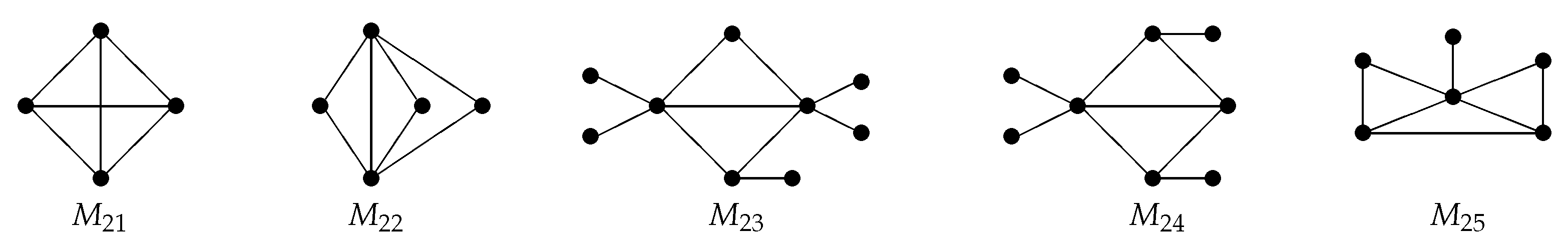
5. 4-Cutwidth Critical Graphs without a Central Vertex and Central Cycle
We now consider the 4-cutwidth critical graphs with neither a central vertex nor a central cycle (see five graphs – in Figure 10).
Theorem 12.
A graph G is 4-cutwidth critical with neither a central vertex nor a central cycle if and only if .
Proof.
Sufficiency. For any , G is needed to show (1) ; (2) for any . These can be done easily, omitted here. On the other hand, we can see that G has neither the central vertex nor the central cycle.
Necessity. Suppose that G is a 4-cutwidth critical graph without central vertex and central cycle, then G has at least two cycles , sharing a common edge. This is because otherwise, G can be thought of as having either a central vertex or a central cycle. So, we have the following:
Claim 2. in Figure 1 is an edge-induced proper subgraph with cutwidth 3 of G.
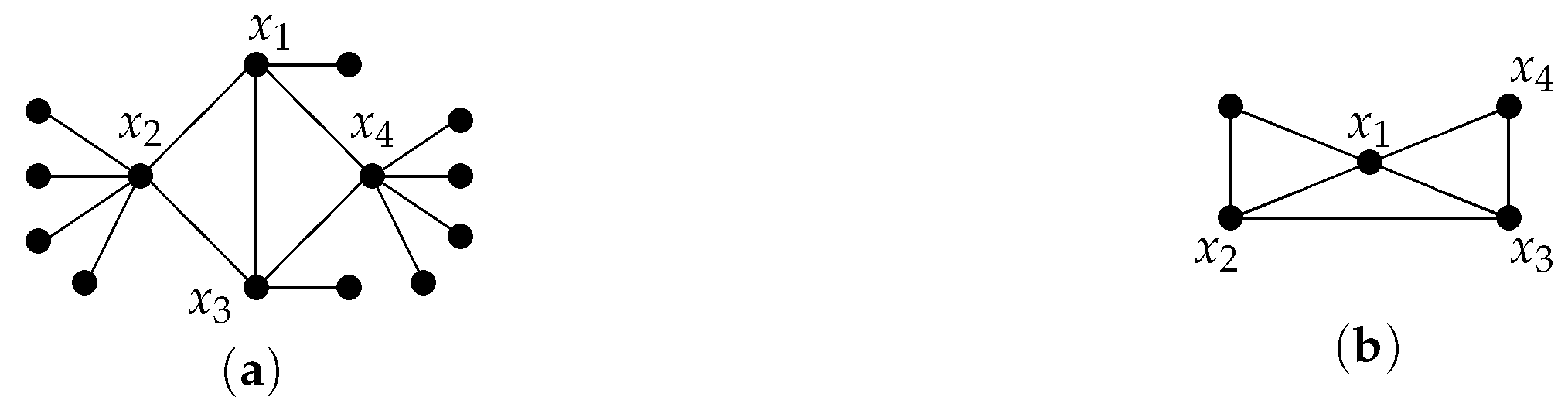
By Claim 2, we have
Claim 3. Suppose that H is a 1-connected and minimum 3-cutwidth graph with , and , in which is maximum for each , then H is graph in Figure 11.
Claim 4. Suppose that H is a 2-connected and minimum noncritical 3-cutwidth graph with , then H is graph in Figure 11.
![Mathematics 11 01631 g011]()
Figure 11.
Two 3-cutwidth graphs containing .

By Claims 3 and 4 and the minimality of G, if G is 1-connected, then G must be one of by direct computations and comparisons. Now, we consider the case that G is 2-connected. Since 4-cutwidth critical graph can be thought of as having a central cycle , we can exclude here. Thus, by direct computations and comparisons, G must be one member of . So, . □
6. Concluding Remarks
In this paper, we have completely characterized the structural properties of 4-cutwidth critical graphs, from which we can see that except for a handful of irregular critical graphs – in Figure 10, the other 4-cutwidth critical graphs can be classified into two classes: graph class with a central vertex , and graph class with a central cycle of length . By means of some ingenious combination, any member of two classes can achieve a subgraph decomposition (or ), in which (or ) is either a 2-cutwith graph or a 3-cutwidth graph for each , or a subgraph decomposition of equal cutwidth 2. For a given integer , although it seems difficult to characterize the detailed structures of k-cutwidth critical graphs, some structural properties of some special graph classes can be found. For instance, using [11], any k-cutwidth critical tree with a central vertex has a subtree decomposition of equal cutwidth , where, for , (or ) is either a -cutwidth critical tree or homeomorphic to a -cutwidth critical tree. Similarly, a k-cutwidth critical non-tree graph also has a subgraph decomposition of equal cutwidth , and are all -cutwidth critical. In the k-cutwidth critical graphs G with a central cycle of length , the structural properties are not yet known. Additionally, for a fixed integer , finding all the -cutwidth critical graph with neither a central vertex nor a central cycle is also a difficult task. All of these are the further objectives to investigate in future works.
Author Contributions
Conceptualization, Z.Z. and H.L.; methodology, Z.Z. and H.L.; formal analysis, Z.Z. and H.L.; investigation, Z.Z. and H.L.; resources, Z.Z. and H.L. writing—original draft preparation, Z.Z.; writing—review and editing, Z.Z. and H.L.; supervision, H.L.; project administration, Z.Z. and H.L.; funding acquisition, Z.Z. All authors have read and agreed to the published version of the manuscript.
Funding
This research was funded by the Soft Science Foundation of the Henan Province of China (192400410212) and partially supported by the Science and Technology Key Project of the Henan Province of China (232102310200).
Institutional Review Board Statement
Not applicable.
Informed Consent Statement
Not applicable.
Data Availability Statement
Not applicable.
Acknowledgments
The authors would like to thank the anonymous referees for their valuable suggestions on improving the quality of this paper.
Conflicts of Interest
The authors declare no conflict of interest.
References
- Bondy, J.A.; Murty, U.S.R. Graph Theory; Springer: New York, NY, USA, 2008. [Google Scholar]
- Diaz, J.; Petit, J.; Serna, M. A survey of graph layout problems. ACM Comput. Surv. 2002, 34, 313–356. [Google Scholar] [CrossRef]
- Garey, M.R.; Johnson, D.S. Computers and Intractability: A Guide to the Theory of NP-Completeness; W.H. Freeman & Company: San Francisco, CA, USA, 1979. [Google Scholar]
- Yannakakis, M. A polynomial algorithm for the min-cut arrangement of trees. J. ACM 1985, 32, 950–989. [Google Scholar] [CrossRef]
- Chung, M.; Makedon, F.; Sudborough, I.H.; Turner, J. Polynomial time algorithms for the min-cut problem on degree restricted trees. SIAM J. Comput. 1985, 14, 158–177. [Google Scholar] [CrossRef]
- Gavril, F. Some NP-complete problems on graphs. In Proceedings of the 11th Conference on Information Sciences and Systems, Baltimore, MD, USA, 30 March–1 April 1977; pp. 91–95. [Google Scholar]
- Monien, B.; Sudborough, I.H. Min-cut is NP-complete for edge weighted trees. Theor. Comput. Sci. 1988, 58, 209–229. [Google Scholar] [CrossRef] [Green Version]
- Lin, Y.; Yang, A. On 3-cutwidth critical graphs. Discret. Math. 2004, 275, 339–346. [Google Scholar] [CrossRef] [Green Version]
- Zhang, Z.; Lai, H. Characterizations of k-cutwidth critical trees. J. Comb. Optim. 2017, 34, 233–244. [Google Scholar] [CrossRef]
- Zhang, Z.; Lai, H. On critical unicyclic graphs with cutwidth four. AppliedMath 2022, 2, 621–637. [Google Scholar] [CrossRef]
- Zhang, Z. Decompositions of critical trees with cutwidth k. Comput. Appl. Math. 2019, 38, 148. [Google Scholar] [CrossRef]
- Zhang, Z.; Zhao, Z.; Pang, L. Decomposability of a class of k-cutwidth critical graphs. Comb. Optim. 2022, 43, 384–401. [Google Scholar] [CrossRef]
- Adolphson, D.; Hu, T.C. Optimal linear ordering. SIAM J. Appl. Math. 1973, 25, 403–423. [Google Scholar] [CrossRef]
- Lengauer, T. Upper and lower bounds on the complexity of the min-cut linear arrangement problem on trees. SIAM J. Alg. Discret. Meth. 1982, 3, 99–113. [Google Scholar] [CrossRef]
- Makedon, F.S.; Sudborough, I.H. On minimizing width in linear layouts. Discret. Appl. Math. 1989, 23, 243–265. [Google Scholar]
- Mutzel, P. A polyhedral approach to planar augmentation and related problems. In European Symposium on Algorithms; volume 979 of Lecture Notes in Computer Science; Spirakis, P., Ed.; Springer: Berlin/Heidelberg, Germany, 1995; pp. 497–507. [Google Scholar]
- Karger, D.R. A randomized fully polynomial time approximation scheme for the all terminal network reliability problem. SIAM J. Comput. 1999, 29, 492–514. [Google Scholar] [CrossRef]
- Botafogo, R.A. Cluster analysis for hypertext systems. In Proceedings of the 16th Annual ACM SIGIR Conference on Research and Development in Information Retrieval, Pittsburgh, PA, USA, 27 June–1 July 1993; pp. 116–125. [Google Scholar]
- Hesarkazzazi, S.; Hajibabaei, M.; Bakhshipour, A.E.; Dittmer, U.; Haghighi, A.; Sitzenfrei, R. Generation of optimal (de)centralized layouts for urban drainage systems: A graph theory based combinatorial multiobjective optimization framework. Sustain. Cities Soc. 2022, 81, 103827. [Google Scholar] [CrossRef]
- Chung, F.R.K. Labelings of Graphs. In Selected Topics in Graph Theory 3; Beineke, L.W., Wilson, R.J., Eds.; Academic Press: London, UK, 1988; pp. 151–168. [Google Scholar]
- Thilikos, D.M.; Serna, M.; Bodlaender, H.L. Cutwidth II: Algorithms for partial w-trees of bounded degree. J. Algorithms 2005, 56, 25–49. [Google Scholar] [CrossRef]
- Korach, E.; Solel, N. Pathwidth and cutwidth. Discret. Appl. Math. 1993, 43, 97–101. [Google Scholar] [CrossRef] [Green Version]
- Chung, F.R.K.; Seymour, P.D. Graphs with small bandwidth and cutwidth. Discret. Math. 1989, 75, 113–119. [Google Scholar] [CrossRef] [Green Version]
Figure 4.
Nine special 4-cutwidth critical graphs.

Figure 5.
Examples of Lemma 14.

Figure 9.
Three 4-cutwidth critical graphs with a .

Figure 10.
4-cutwidth critical graphs without a central vertex and central cycle.

Disclaimer/Publisher’s Note: The statements, opinions and data contained in all publications are solely those of the individual author(s) and contributor(s) and not of MDPI and/or the editor(s). MDPI and/or the editor(s) disclaim responsibility for any injury to people or property resulting from any ideas, methods, instructions or products referred to in the content. |
© 2023 by the authors. Licensee MDPI, Basel, Switzerland. This article is an open access article distributed under the terms and conditions of the Creative Commons Attribution (CC BY) license (https://creativecommons.org/licenses/by/4.0/).
Share and Cite
MDPI and ACS Style
Zhang, Z.; Lai, H. Structures of Critical Nontree Graphs with Cutwidth Four. Mathematics 2023, 11, 1631. https://doi.org/10.3390/math11071631
AMA Style
Zhang Z, Lai H. Structures of Critical Nontree Graphs with Cutwidth Four. Mathematics. 2023; 11(7):1631. https://doi.org/10.3390/math11071631
Chicago/Turabian StyleZhang, Zhenkun, and Hongjian Lai. 2023. "Structures of Critical Nontree Graphs with Cutwidth Four" Mathematics 11, no. 7: 1631. https://doi.org/10.3390/math11071631
Note that from the first issue of 2016, this journal uses article numbers instead of page numbers. See further details here.