Article

Fractional-Modified Bessel Function of the First Kind of Integer Order

1
Faculty of Science, University of Zaragoza, Pedro Cerbuna, 50009 Zaragoza, Spain
2
Institute of Interdisciplinary Physics and Complex Systems (IFISC), 07122 Palma de Mallorca, Spain
*
Author to whom correspondence should be addressed.
Mathematics 2023, 11(7), 1630; https://doi.org/10.3390/math11071630
Submission received: 15 February 2023 / Revised: 19 March 2023 / Accepted: 24 March 2023 / Published: 28 March 2023
(This article belongs to the Special Issue Mathematics: 10th Anniversary)

Abstract

:
The modified Bessel function (MBF) of the first kind is a fundamental special function in mathematics with applications in a large number of areas. When the order of this function is integer, it has an integral representation which includes the exponential of the cosine function. Here, we generalize this MBF to include a fractional parameter, such that the exponential in the previously mentioned integral is replaced by a Mittag–Leffler function. The necessity for this generalization arises from a problem of communication in networks. We find the power series representation of the fractional MBF of the first kind as well as some differential properties. We give some examples of its utility in graph/networks analysis and mention some fundamental open problems for further investigation.

1. Introduction

The modified Bessel function (MBF) of the first kind of order ν , denoted by I ν ( z ) is defined by [1,2,3]
I ν ( z ) = ( z 2 ) ν k = 0 1 Γ ( k + 1 ) Γ ( k + ν + 1 ) ( z 2 ) 2 k ,
for an unrestricted real (or complex) number ν , where Γ ( · ) is the Euler gamma function, which is defined by
Γ ( z ) : = 0 t z 1 e t d t , R ( z ) > 0 .
The MBF of the first kind is one of the linearly independent solutions of the differential equation
z 2 u ( z ) + z u ( z ) ( z 2 + ν 2 ) u ( z ) = 0 ,
which frequently appears in mathematical physics. Then, it is common to find this function related to a large variety of applications, such as elasticity [4], imaging [5,6], sport data [7], and statistics [8], to mention just a few. In particular, when ν Z , the MBF of the first kind has the following integral representation:
I ν ( z ) = 1 π 0 π e z cos θ cos ( ν θ ) d θ ,
which appears in the analytical expression of the so-called Estrada index of an infinite linear and of an infinite circular graph [9]. The importance of the MBF of the first kind is also reflected by the fact that a large number of publications in mathematics deal with the properties of these functions (see [10,11,12,13,14,15,16,17,18] for some recent examples).
Here, we propose a fractional generalization of the MBF of the first kind. This function, which we will call fractional MBF (FMBF) of the first kind, is found in the analytical calculations of communicability [19,20] and related indices [21] in certain classes of infinite graphs. Therefore, it is not proposed in an ad hoc way as in other previous cases [22] but in the context of the study of graphs and networks. We introduce the context in which the FMBF of the first kind arises and then study some of its properties, such as its power series, convergence and recurrence relations. We hope these functions and other related ones play a fundamental role in the study of fractional analogous of Bessel functions and their applications.

2. Preliminaries

It is known that the MBF of the first kind satisfies the following three terms’ recurrence:
I ν 1 ( z ) I ν + 1 ( z ) = 2 ν z I ν ( z ) .
In addition, the derivative of the MBF of the first kind has the following well-known recurrence relations:
d d z ( z ν I ν ( z ) ) = z ν I ν 1 ( z ) ,
d d z ( z ν I ν ( z ) ) = z ν I ν + 1 ( z ) ,
d d z I ν ( z ) = 1 2 ( I ν 1 ( z ) + I ν + 1 ( z ) ) .
First, we will rewrite these recurrence formulas for the MBF of the first kind in the following way. We apply the classical rule of derivation for a product to Equation (6) and obtain
d d z ( z ν I ν ( z ) ) = ν z ν 1 I ν ( z ) + z ν d d z I ν ( z ) ,
such that we can write
d d z I ν ( z ) = I ν 1 ( z ) ν z I ν ( z ) .
Similarly, we have
d d z I ν ( z ) = I ν + 1 ( z ) + ν z I ν ( z ) .
We now consider the Caputo fractional derivative which we will use in this work. We start by defining the Riemann–Liouville integral, which for a locally integrable function f ( t ) , a parameter γ representing the fractional order, is written as [23]
I 0 , t γ f ( t ) = 1 Γ ( γ ) 0 t f ( τ ) ( t τ ) 1 γ d τ γ > 0 ,
where it can be easily proved that lim γ 0 I 0 , t γ f ( t ) = f ( t ) . Now, let α ( 0 , + ) be the fractional ordering parameter and let m : = α , where . is the ceiling function, the Caputo derivative of f ( t ) , for which f ( t ) = 0 , if t < 0 , is defined as [23]:
D 0 , t α f ( t ) = I 0 , t ( m α ) f ( m ) ( f ( t ) ) = 1 Γ ( m α ) 0 t f ( m ) ( τ ) ( t τ ) α + 1 m d τ .
Here, we consider only the cases where α ( 0 , 1 ] and γ [ 0 , 1 ) for the Caputo derivative and Riemann–Liouville integral, respectively. Hereafter, we will consider (13) for m = 1 , which we will write with the following notation:
D t α f ( t ) = 1 Γ ( 1 α ) 0 t f ( τ ) ( t τ ) α d τ ; α ( 0 , 1 ) .
The following results are possibly proved elsewhere, and we show them here for the sake of self-containment of our work. Let α ( 0 , 1 ) and let f ( t ) = n = 0 a n t n be a power series with convergence radius R ( 0 , + ] . Then,
D x α f ( x ) = D x α ( n = 0 a n x n ) = n = 0 a n D x α x n ,
I α f ( x ) = I α ( n = 0 a n x n ) = n = 0 a n I α x n .
We also provide a few other properties of the Caputo derivative and of the Riemann–Liouville integral which are useful in the proof of our results.
  • Let spanish α ( 0 , 1 ] and C R , then: D t α ( C ) = 0 ;
  • Let α ( 0 , 1 ] and r > 0 , then D t α ( t r ) = Γ ( r + 1 ) Γ ( r α + 1 ) t r α ;
  • Let γ [ 0 , 1 ) and r > 1 , then I γ ( t r ) = Γ ( r + 1 ) Γ ( r + γ + 1 ) t r + γ ;
  • Let γ ( 0 , 1 ) and r > 0 , then D t γ ( I γ ( t r ) ) = I γ ( D t γ ( t r ) ) = t r .

3. Fractional Communicability in Graphs

Let G = ( V , E ) be a simple, finite, connected graph where V is the set of vertices and E is the set of edges. Let A be the adjacency matrix of G . Let v , w V be two nodes of G. Then, the communicability function Γ v , w ( ζ , G ) of the graph with parameter ζ R is known to be
Γ v , w ( ζ , G ) = k = 0 ζ k ( A k ) v w Γ ( k + 1 ) = ( exp ( ζ A ) ) v w .
When v = w , the self-communicability of the node v is known as the subgraph centrality of that node and the sum of all subgraph centralities in the graph is the so-called Estrada index: E E ( ζ , G ) = t r exp ( ζ A ) , where t r is the trace of the matrix. The communicability function and the Estrada index can be derived in different theoretical contexts studying dynamical systems on graphs. This includes, for instance, a linearized yet stable susceptible-infected epidemiological model, tight-binding models in quantum mechanics, thermal Green’s function of system of quantum harmonic oscillators as well as in synchronization of networks. In all of them, the parameter ζ R acquires different “physical” meanings.
Let us make the following generalization of the communicability function:
( E α , β ( ζ , G ) ) v , w : = k = 0 ζ k ( A k ) v w Γ ( α k + β ) ,
which is equal to the standard communicability function when α = β = 1 . Evidently, this function corresponds to the v , w entry of the Mittag–Leffler matrix function of ζ A . This function, particularly E α , 1 ( ζ , G ) has been found in the analytical solution of the fractional version of the linearized yet stable susceptible-infected epidemiological model, where the standard time derivative has been replaced by the Caputo fractional one. That is, let x i be the probability that a node i V in G becomes infected from a contagious disease circulating the graph. If the birth rate of the disease is β , then the fractional Susceptible–Infected model developed in [24] is given by
D t α ( log ( 1 x i ) ) ( t ) = β α j A i j x j ( t ) , x i ( 0 ) = x 0 i [ 0 , 1 ) .
Then, under certain plausible initial conditions γ = 1 c / n (c is a constant and n is the number of vertices) on the graph, the vector of solutions of this model is given by:
x = ( 1 γ γ ) E α , 1 ( t α β α γ A ) 1 ( 1 γ γ + log γ ) 1 ,
where 1 is a vector of ones.
Other more ad hoc encounters with these functions have recently appeared in the literature by Arrigo and Durastante [25] and reviewed by Estrada [26] in the context of the so-called “Estrada indices”. Hereafter, we will call ( E α , β ( ζ , G ) ) v , w the fractional communicability between the corresponding nodes. When v = w , we will call it the fractional subgraph centrality of the node, and the index defined by t r ( E α , β ( ζ , G ) ) the Estrada–Mittag–Leffler index of the graph [26]. From now on, we will focus only on the cases where β = 1 and we will use the notation E α ( ζ , G ) for E α , β = 1 ( ζ , G ) .

4. Fractional Communicabilities in Path and Cycle Graphs

Let us start with the following.
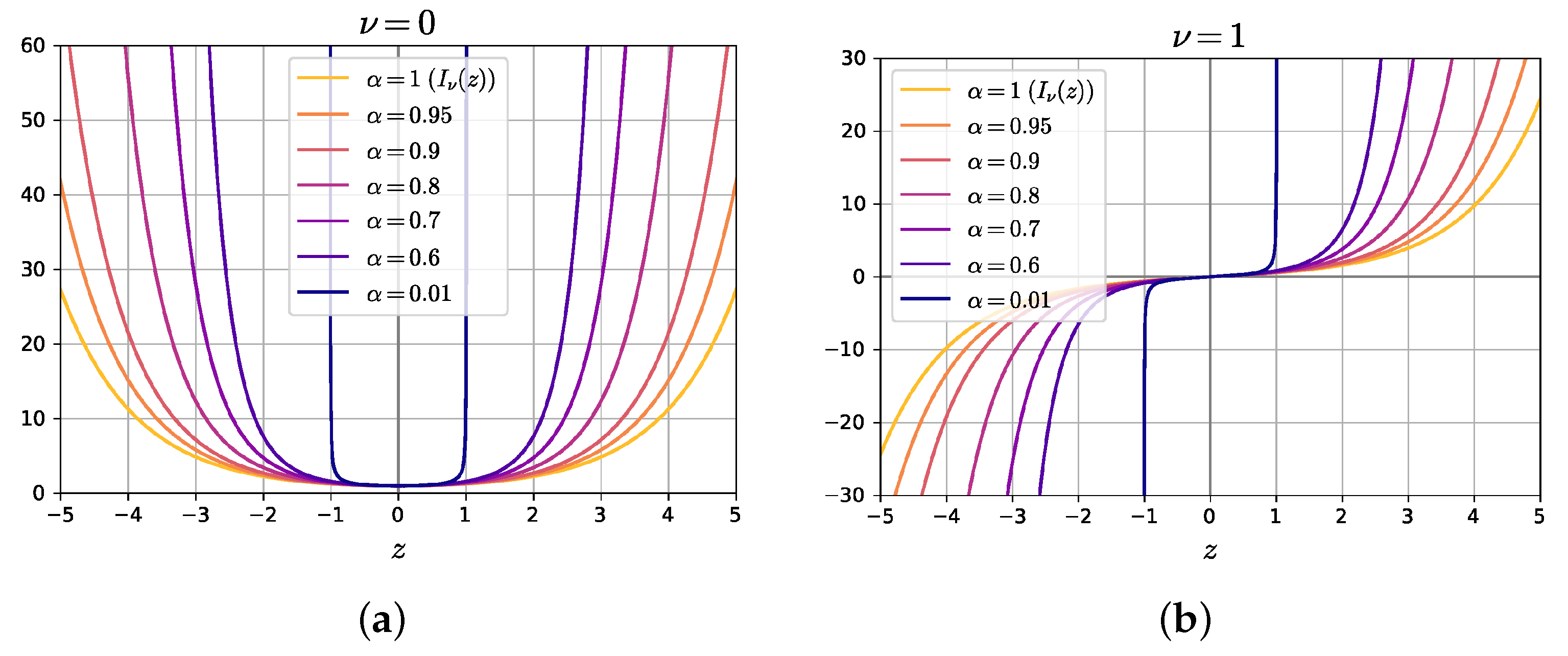
Definition 1. 
Let E α ( z ) be the Mittag–Leffler function of z . Then, we define the following integral:
E ν , α ( z ) : = 1 π 0 π cos ( ν θ ) E α ( z cos θ ) d θ , ν Z ,
Remark 1. 
Notice that E ν , α = 1 ( z ) = 1 π 0 π e z cos θ cos ( ν θ ) d θ = : I ν ( z ) which is the modified Bessel function of the first kind. Therefore, E ν , α ( z ) is the fractional analogous of I ν ( z ) and will be named here as the fractional modified Bessel function of the first kind (see plots in Figure 1).
Remark 2. 
Notice that the FMBF of the first kind also satisfies similar recurrence relations as the not fractional one. That is,
E ν 1 , α ( z α ) E ν + 1 , α ( z α ) = 2 α ν · I 1 α ( z 1 · E ν , α ( z α ) ) .
Let G be a path graph on n nodes P n , i.e., the graph in which all nodes have degree two but two nodes that have degree one. Without any loss of generality, we will take ζ = 1 from now on. Then, we can now prove the following result.
Theorem 1. 
Let v and w be two nodes of the path graph of n nodes P n and let ( E α ( P n ) ) v w be the Mittag–Leffler communicability between nodes v and w. Let,
( E ^ α ( P n ) ) v w = E v w , α ( 2 ) E v + w , α ( 2 ) v w E 0 , α ( 2 ) E 2 r ( v ) , α ( 2 ) v = w ,
where
r ( p ) = v i f v n / 2 ( n even ) or v ( n + 1 ) / 2 ( n odd ) n v + 1 if v > n / 2 ( n even ) or v > ( n + 1 ) / 2 ( n odd ) .
Then, when the number of nodes is sufficiently large, i.e., when n , the value of ( E ^ α ( P n ) ) v w tends to the actual value of the communicability function for a pair of nodes in P n , which mathematically is expressed as: lim n ( E α ( P n ) ) v w / ( E ^ α ( P n ) ) v w = 1 .
Proof. 
Let us recall that in a path graph of n nodes, the eigenvalues of the adjacency matrix are given by
λ j ( P n ) = 2 cos ( j π n + 1 ) ,
and the pth entry of the jth eigenvector is
ψ j ( p ) = 2 n + 1 sin ( j p π n + 1 ) .
By replacing these spectral values on the expression of ( E α ( A ) ) v w , we obtain
( E α ( P n ) ) v w = 1 n + 1 j = 1 n ( cos ( j π ( v w ) n + 1 ) cos ( j π ( v + w ) n + 1 ) ) E α ( 2 cos ( j π n + 1 ) ) .
Let
( E ^ α ( P n ) ) v w : = 1 π 0 π cos ( θ ( v w ) ) E α ( 2 cos θ ) d θ 1 π 0 π cos ( θ ( v + w ) ) E α ( 2 cos θ ) d θ = E v w , α ( 2 ) E v + w , α ( 2 )
where θ : = j π n + 1 . When v = w , let
( E ^ α ( P n ) ) v v : = 1 π 0 π [ 1 cos ( 2 v θ ) ] E α ( 2 cos ( θ ) ) = E 0 , α ( 2 ) E 2 r ( v ) , α ( 2 ) ,
where the term r ( p ) arises due to the equivalence between the nodes labeled as i and n i + 1 . The relationship between ( E ^ α ( P n ) ) v v and ( E α ( P n ) ) v w can be seen as the one existing in numerical methods such as the trapezium or Simpson’s rules in which an integral is approximated by a summation. Here the analogous of the number of strips used in those numerical methods of integration is the number of nodes in the path. Then, it is easy to realize that when the number of nodes is sufficiently large, we have lim n ( E α ( P n ) ) v w / ( E ^ α ( P n ) ) v w = 1 . □
Following the same scheme of proof, we can show the following.
Theorem 2. 
Let v and w be two nodes of the cycle graph of n nodes C n and let ( E α ( C n ) ) v w be the Mittag–Leffler communicability between nodes v and w. Let
( E ^ α ( C n ) ) v w = E d v w , α ( 2 ) ,
where d v w is the shortest path distance between the two nodes, (notice that d v v = 0 ). Then, when the number of nodes is sufficiently large, i.e., when n , the value of ( E ^ α ( C n ) ) v w tends to the actual value of the communicability function for a pair of nodes in C n , which means that
lim n ( E α ( C n ) ) v w / ( E ^ α ( C n ) ) v w = 1 .
Example 1. 
We calculate the values of ( E α ( P n ) ) v , v and ( E α ( C n ) ) v , v as well as their approximation based on the FMBF of the first kind ( E ^ α ( P n ) ) v , v and ( E ^ α ( C n ) ) v , v for n = 5 , 20 , 40 , 60 , 80 , 100 . In Table 1, we give the values of these indexes for the first three nodes of the path graph (labeled 1, 2 and 3, respectively, starting from one end) with n = 20 and for any node of the cycle graph (all are equivalent). The results for n > 20 in P n and those for n > 40 in C n do not differ significantly (up to the seventh decimal place) from those for n = 20 or n = 40 , respectively. The important result here is that for relatively large n, the approximate values based on the FMBF of the first kind are indistinguishable from those based on the Mittag–Leffler matrix function.
The previous results show that the fractional modified Bessel function (FMBF) of the first kind appears in the expression of the fractional communicability between any pair of nodes in path and cycle graphs when the number of nodes is very large. Therefore, we will focus now on some of the most important properties of this new function.

5. On the Estrada–Mittag–Leffler Indices of P n and C n

By the definition of the Estrada index, we have that the Estrada–Mittag–Leffler index (see [25,26]) is defined as
E E α ( G ) = v = 1 n ( E α ( G ) ) v v = j = 1 n E α ( λ j ) .
Then, for a cycle C n , we have:
E E α ( C n ) = j = 1 n E α ( 2 cos ( 2 j π n ) ) = n ( 1 n j = 1 n E α ( 2 cos ( 2 j π n ) ) ) .
Let
E E α ^ ( C n ) : = n ( 1 2 π 0 2 π E α ( 2 cos z ) d z ) = n ( 1 π 0 π E α ( 2 cos z ) d z ) n · E α , 0 ( 2 ) .
Then, when the number of nodes is sufficiently large, i.e., when n , the value of E ^ α ( P n ) tends to the actual value of the Estrada–Mittag–Leffler index in C n , lim n E E α ( C n ) / E E α ^ ( C n ) = 1 .
For the case of the path graph, we have:
E E α ( P n ) = k = 1 n E α ( 2 cos ( k π n + 1 ) ) = 1 2 k = 0 n E α ( 2 cos ( k π n + 1 ) ) + 1 2 k = 1 n + 1 E α ( 2 cos ( k π n + 1 ) ) 1 2 ( E α ( 2 ) + E α ( 2 ) ) = n + 1 2 ( 1 n + 1 k = 0 n E α ( 2 cos ( k π n + 1 ) ) ) + n + 1 2 ( 1 n + 1 k = 1 n + 1 E α ( 2 cos ( k π n + 1 ) ) ) 1 2 ( E α ( 2 ) + E α ( 2 ) ) .
Let
E E α ^ ( P n ) : = n + 1 2 ( 1 π 0 π E α ( 2 cos z ) d z ) + n + 1 2 ( 1 π 0 π E α ( 2 cos z ) d z ) 1 2 ( E α ( 2 ) + E α ( 2 ) ) = ( n + 1 ) E α , 0 ( 2 ) 1 2 ( E α ( 2 ) + E α ( 2 ) ) .
Then, when the number of nodes is sufficiently large, i.e., when n , the value of E E α ( P n ) tends to the actual value of the Estrada–Mittag–Leffler index in P n , lim n E E α ( P n ) / E E α ^ ( P n ) = 1 .

6. Power Series of the the FMBF of the First Kind

We start by expressing the FMBF of the first kind as a power series.
Lemma 1. 
Let E ν , α ( z ) be the fractional modified Bessel function of the first kind of z with fractional parameter α and ν Z . Then,
E ν , α ( z ) = k = 0 ( 2 k + ν ) ! Γ ( α ( 2 k + ν ) + 1 ) k ! ( k + ν ) ! ( z 2 ) 2 k + ν .
Proof. 
First, we use the Taylor series expression of the Mittag–Leffler function on the definition of E ν , α :
E ν , α ( z ) = 1 π 0 π j = 0 z j cos j ( θ ) Γ ( α j + 1 ) cos ( ν θ ) d θ = j = 0 [ z j π Γ ( α k + 1 ) 0 π cos j ( θ ) cos ( ν θ ) d θ ]
To obtain the value of the integral, we equalize E ν , α ( z ) to I ν ( z ) for α = 1 , such that we obtain:
0 π cos ( θ ) j cos ( ν θ ) d θ = π · j ! ( j ν 2 ) ! ( j + ν 2 ) ! 2 j if j ν and j + ν is e v e n 0 otherwise
Finally, we replace the solution of this integral into E ν , α ( z ) , and we are finished. □
Remark 3. 
When α = 1 the term Γ ( α k + 1 ) = k ! and E ν , α = 1 ( z ) = I ν ( z ) .
Lemma 2. 
The power series
k = 0 ( ν + 2 k ) ! Γ ( α ( ν + 2 k ) + 1 ) 1 k ! ( ν + k ) ! ( z 2 ) 2 k + ν
converges z if α ( 0 , 1 ] and in the limiting case when α = 0 , it converges if z < 1 and diverges if z > 1 .
Proof. 
Let us consider the coefficients a j ( ν , α ) , which are given by:
a j ( ν , α ) = ( ν + 2 k ) ! Γ ( α ( ν + 2 k ) + 1 ) 1 k ! ( ν + k ) ! 1 2 2 k + ν if j = 2 k + ν , k Z + 0 otherwise
We apply the Cauchy–Hadamard theorem to calculate the convergence radius R ( ν , α ) of the series, which is defined as
R ( ν , α ) = 1 lim sup j ( a j ( ν , α ) 1 / j )
On the upper limit, there is only influence of the values of j = 2 k + ν . Thus, when k , we have
lim sup j ( a j ( ν , α ) 1 / j ) = lim sup k ( a 2 k + ν ( ν , α ) 1 / ( 2 k + ν ) ) = lim k ( a 2 k + ν ( ν , α ) 1 / ( 2 k + ν ) )
Using Stirling approximation, the following limit can be obtained for α ( 0 , 1 ] (see Remark 4):
lim k a 2 k + ν ( ν , α ) 1 / ( 2 k + ν ) = lim k ( e α ( ν + 2 k ) ) α = 0
Therefore, when α ( 0 , 1 ] we obtain that R ( ν , α ) = + , indicating global convergence of the series. Now, when α = 0 , we have that
a 2 k + ν ( ν , 0 ) = ( ν + 2 k ) ! k ! ( ν + k ) ! 1 2 2 k + ν
From this equation, it can be proved that (see Remark 5):
lim k a 2 k + ν ( ν , α ) 1 / ( 2 k + ν ) = lim k ( ν + 2 k k ( ν + k ) ) 1 2 k + ν = 1
Therefore, R ( ν , 0 ) = 1 , such that (40) converges for z if z < 1 and does not converge if z > 1 . □
Remark 4. 
In the proof of Lemma 2, we take into account Stirling approximation for both the factorial and the gamma function Γ. This approximation allows us to replace terms of the form n ! and Γ ( z + 1 ) by n n e n 2 π n and z z e z 2 π z , respectively, when both n and z tend to + .
lim k a 2 k + ν ( ν , α ) 1 2 k + ν = lim k ( ( ν + 2 k ) ! Γ ( α ( ν + 2 k ) + 1 ) 1 k ! ( ν + k ) ! 1 2 2 k + ν ) 1 2 k + ν = lim k ( ( ν + 2 k ) ν + 2 k e ( ν + 2 k ) 2 π ( ν + 2 k ) ( α ( ν + 2 k ) ) α ( ν + 2 k ) e α ( ν + 2 k ) 2 π α ( ν + 2 k ) e k e ν + k k k ( ν + k ) ν + k 2 π k ( ν + k ) 1 2 2 k + ν ) 1 2 k + ν = lim k ( ( ν + 2 k ) ν + 2 k k k ( ν + k ) ν + k 2 2 k + ν · 1 2 π α k ( ν + k ) · e α ( ν + 2 k ) · 1 ( α ( ν + 2 k ) ) α ( ν + 2 k ) ) 1 2 k + ν
It is easy to study the correspondent limit for the first and second factor of the previous expression:
lim k ( ( ν + 2 k ) ν + 2 k k k ( ν + k ) ν + k 2 2 k + ν ) 1 2 k + ν = 1 2 lim k ν + 2 k ν + k ( ν + k k ) k 2 k + ν = lim k ( 1 + ν k ) k 2 k + ν = 1
lim k ( 1 2 π α k ( ν + k ) ) 1 2 k + ν = lim k ( α k ( ν + k ) ) 1 2 k + ν = 1
Therefore:
lim k a 2 k + ν ( ν , α ) 1 2 k + ν = lim k ( e α ( ν + 2 k ) ( α ( ν + 2 k ) ) α ( ν + 2 k ) ) 1 2 k + ν = lim k ( e α ( ν + 2 k ) ) α = 0 .
Remark 5. 
In the proof of Lemma 2, we also considered the following
lim k a 2 k + ν ( ν , 0 ) 1 2 k + ν = lim k ( ( ν + 2 k ) ! k ! ( ν + k ) ! 1 2 2 k + ν ) 1 2 k + ν = lim k ( ( ν + 2 k ) ν + 2 k e ( ν + 2 k ) 2 π ( ν + 2 k ) k k e k 2 π k ( ν + k ) ν + k e ( ν + k ) 2 π ( ν + k ) 1 2 2 k + ν ) 1 2 k + ν = lim k ( ( ν + 2 k ) ν + 2 k k k ( ν + k ) ν + k 2 2 k + ν ( ν + 2 k ) 2 π k ( ν + k ) ) 1 2 k + ν .
As it was shown in the Remark 4, the first of the two previous factors tends to one as k . Therefore:
lim k a 2 k + ν ( ν , 0 ) 1 2 k + ν = lim k ( ( ν + 2 k ) k ( ν + k ) ) 1 2 k + ν = 1 .

7. Differential Properties of the FMBF of the First Kind

We now obtain recurrence relations for the Caputo derivatives of E ν , α ( z α ) .
Theorem 3. 
The following equalities hold
  • D z α ( E ν , α ( z α ) ) = E ν 1 , α ( z α ) α ν · I 1 α ( z 1 · E ν , α ( z α ) )
  • D z α ( E ν , α ( z α ) ) = E ν + 1 , α ( z α ) + α ν · I 1 α ( z 1 · E ν , α ( z α ) )
  • D z α ( E ν , α ( z α ) ) = 1 2 ( E ν 1 , α ( z α ) + E ν + 1 , α ( z α ) ) .
Before proceeding with the proof, we need to state the following auxiliary result.
Lemma 3. 
Let α ( 0 , 1 ] and ν N , then:
α · I 1 α ( z 1 · E ν , α ( z α ) ) = k = 0 1 Γ ( α ( 2 k + ν 1 ) + 1 ) ( 2 k + ν 1 ) ! k ! ( k + ν ) ! 1 2 2 k + ν z α ( 2 k + ν 1 )
Proof. 
The expression (16) allows us to calculate spanish I 1 α ( z 1 · E ν , α ( z α ) ) by integrating partially each term of the power series. This operation can be applied to powers of z with an exponent larger than 1 . Then, because we are considering only the cases where γ N , it is always true that α ( 2 k + ν ) 1 > 1 for all possible k and ν , such that:
α · I 1 α ( z 1 · E ν , α ( z α ) ) = α · k = 0 1 Γ ( α ( 2 k + ν ) + 1 ) ( 2 k + ν ) ! k ! ( k + ν ) ! 1 2 2 k + ν I 1 α ( z α ( 2 k + ν ) 1 ) .
Using properties of the Riemann–Liouville integral when r = α ( 2 k + ν ) 1 and γ = 1 α ( 0 , 1 ) , we have:
I 1 α ( z α ( 2 k + ν ) 1 ) = Γ ( α ( 2 k + ν ) 1 + 1 ) Γ ( α ( 2 k + ν ) 1 + 2 α ) z α ( 2 k + ν ) 1 + 1 α = Γ ( α ( 2 k + ν ) ) Γ ( α ( 2 k + ν 1 ) + 1 ) z α ( 2 k + ν 1 )
Plugging (58) in (57), we obtain the result. □
We now proceed with the proof of Theorem 3.
Proof. 
We start by proving the recurrence (1). For that, we take into account the property (2) with r = α ( 2 k + ν ) to show that:
D z α ( E ν , α ( z α ) ) = k = 0 1 Γ ( α ( 2 k + ν ) + 1 ) ( 2 k + ν ) ! k ! ( k + ν ) ! 1 2 2 k + ν D z α ( z α ( 2 k + ν ) ) = k = 0 1 Γ ( α ( 2 k + ν 1 ) + 1 ) ( 2 k + ν ) ! k ! ( k + ν ) ! 1 2 2 k + ν z α ( 2 k + ν 1 ) = k = 0 ( 2 k + ν k + ν ) 1 Γ ( α ( 2 k + ν 1 ) + 1 ) ( 2 k + ν 1 ) ! k ! ( k + ν 1 ) ! 1 2 2 k + ν z α ( 2 k + ν 1 ) = k = 0 ( 1 1 2 ν k + ν ) 1 Γ ( α ( 2 k + ν 1 ) + 1 ) ( 2 k + ν 1 ) ! k ! ( k + ν 1 ) ! 1 2 2 k + ν 1 z α ( 2 k + ν 1 ) = E ν 1 , α ( z α ) k = 0 ν k + ν 1 Γ ( α ( 2 k + ν 1 ) + 1 ) ( 2 k + ν 1 ) ! k ! ( k + ν 1 ) ! 1 2 2 k + ν z α ( 2 k + ν 1 ) = E ν 1 , α ( z α ) ν k = 0 1 Γ ( α ( 2 k + ν 1 ) + 1 ) ( 2 k + ν 1 ) ! k ! ( k + ν ) ! 1 2 2 k + ν z α ( 2 k + ν 1 ) = E ν 1 , α ( z α ) Ξ .
We now consider the term Ξ , which by using the auxiliary result (3) gives the following:
Ξ = ν k = 0 1 Γ ( α ( 2 k + ν 1 ) + 1 ) ( 2 k + ν 1 ) ! k ! ( k + ν ) ! 1 2 2 k + ν z α ( 2 k + ν 1 ) = α ν · I 1 α ( z 1 · E ν , α ( z α ) ) ,
which proves (1). Let us now prove (2). Let ν N and using again the property (2) with r = α ( 2 k + ν ) , we write
D z α ( E ν , α ( z α ) ) = k = 0 1 Γ ( α ( 2 k + ν ) + 1 ) ( 2 k + ν ) ! k ! ( k + ν ) ! 1 2 2 k + ν D z α ( z α ( 2 k + ν ) ) = k = 0 1 Γ ( α ( 2 k + ν 1 ) + 1 ) ( 2 k + ν ) ! k ! ( k + ν ) ! 1 2 2 k + ν z α ( 2 k + ν 1 ) = k = 0 ( 2 k + ν k + ν ) 1 Γ ( α ( 2 k + ν 1 ) + 1 ) ( 2 k + ν 1 ) ! k ! ( k + ν 1 ) ! 1 2 2 k + ν z α ( 2 k + ν 1 ) = k = 0 2 k k + ν 1 Γ ( α ( 2 k + ν 1 ) + 1 ) ( 2 k + ν 1 ) ! k ! ( k + ν 1 ) ! 1 2 2 k + ν z α ( 2 k + ν 1 ) A + k = 0 ν k + ν 1 Γ ( α ( 2 k + ν 1 ) + 1 ) ( 2 k + ν 1 ) ! k ! ( k + ν 1 ) ! 1 2 2 k + ν z α ( 2 k + ν 1 ) B
Let us rewrite now the expression for A by observing that the contribution for k = 0 is zero, so that we start the summation by k = 1 :
A = k = 1 2 k k + ν 1 Γ ( α ( 2 k + ν 1 ) + 1 ) ( 2 k + ν 1 ) ! k ! ( k + ν 1 ) ! 1 2 2 k + ν z α ( 2 k + ν 1 ) = k = 1 1 Γ ( α ( 2 k + ν 1 ) + 1 ) ( 2 k + ν 1 ) ! ( k 1 ) ! ( k + ν ) ! 1 2 2 k + ν 1 z α ( 2 k + ν 1 ) = k = 1 1 Γ ( α ( 2 ( k 1 ) + ν + 1 ) + 1 ) ( 2 ( k 1 ) + ν + 1 ) ! ( k 1 ) ! ( k 1 + ν + 1 ) ! 1 2 2 ( k 1 ) + ν + 1 z α ( 2 ( k 1 ) + ν + 1 ) .
We now identify the indexspanish k 1 as the initial point in the summation such that we can start it at 0, so that
k = 0 1 Γ ( α ( 2 k + ν + 1 ) + 1 ) ( 2 k + ν + 1 ) ! k ! ( k + ν + 1 ) ! 1 2 2 k + ν + 1 z α ( 2 k + ν + 1 ) = E ν + 1 , α ( z α )
It is easy to check that the term B is just the term Ξ used in the proof of the previous recurrence. Thus, we have that
B = α ν · I 1 α ( z 1 · E ν , α ( z α ) ) ,
which gives us the result for recurrence (2). Finally, for recursion (3), we have
2 D z α ( E ν , α ( z α ) ) = E ν + 1 , α ( z α ) + α ν · I 1 α ( z 1 · E ν , α ( z α ) ) + E ν 1 , α ( z α ) α ν · I 1 α ( z 1 · E ν , α ( z α ) ) = E ν + 1 , α ( z α ) + E ν 1 , α ( z α ) ,
which finally proves the result. □
Remark 6. 
Theorem 3 generalizes the recurrence formulae obtained for the standard Bessel function of the first kind. That is, when α = 1 , the expressions in Theorem 3 transform into the recurrence formulas for the MBF of the first kind given in the Introduction.

8. Open Problems

Here, we have proposed a generalization of MBF of the first kind I ν ( z ) when ν Z , which transforms the integral representation
I ν ( z ) = 1 π 0 π e z cos θ cos ( ν θ ) d θ ,
into E ν , α ( z ) , which for ν Z has the following representation:
E ν , α ( z ) = 1 π 0 π E α , 1 ( z cos θ ) cos ( ν θ ) d θ .
Therefore, the first extension of the current work is to generalize E ν , α ( z ) for ν R . This extension can be obtained by starting from the power series expression of the FMBF of the first kind obtained here. The focus in the current work has been on the restricted domain of ν Z , which is the one that naturally emerges from the problem of considering the fractional analogous to the communicability functions in simple graphs such as the path and cycle of n nodes.
A second generalization is obviously to consider the more general form of the Mittag–Leffler function such that:
E ν , α , β ( z ) = 1 π 0 π E α , β ( z cos θ ) cos ( ν θ ) d θ .

Author Contributions

Methodology, E.E.; Formal analysis, A.M. and E.E.; Writing—original draft, E.E.; Writing—review & editing, E.E.; Supervision, E.E. All authors have read and agreed to the published version of the manuscript.

Funding

Project OLGRA (PID2019-107603GB-I00) funded by the Spanish Ministry of Science and Innovation as well as the Maria de Maeztu project CEX2021-001164-M funded by the MCIN/AEI/ 10.13039/501100011033.

Data Availability Statement

No data was used in this paper.

Conflicts of Interest

The authors declare no conflict of interest.

References

  1. Lebedev, N.N. Special Functiones and Their Applications; Dover Pub. Inc.: New York, NY, USA, 1972; p. 108. [Google Scholar]
  2. Bowman, F. Introduction to Bessel Functions; Dover Pub. Inc.: New York, NY, USA, 1958; p. 41. [Google Scholar]
  3. Watson, G.N. A Treatise on the Theory of Bessel Functions; Cambridge Mathematical Library: New York, NY, USA, 1995; p. 77. [Google Scholar]
  4. Simpson, H.; Spector, S. Some monotonicity results for ratios of modified Bessel functions. J. Inequal. Appl. 1984, 42, 95–98. [Google Scholar] [CrossRef] [Green Version]
  5. Hwang, Y. Difference-Based Image Noise Modeling Using Skellam Distribution. IEEE Trans. Pattern Anal. Mach. Intell. 2012, 34, 1329–1341. [Google Scholar] [CrossRef] [PubMed]
  6. Wolfe, P.; Hirakawa, K. Efficient Multivariate Skellam Shrinkage for Denoising Photon-Limited Image Data: An Empirical Bayes Approach. In Proceedings of the 16th IEEE International Conference on Image Processing (ICIP-09), Cairo, Egypt, 7–10 November 2009; pp. 2961–2964. [Google Scholar]
  7. Karlis, D.; Ntzoufras, I. Analysis of sports data using bivariate Poisson models. J. R. Stat. Soc. Ser. D 2003, 52, 381–393. [Google Scholar] [CrossRef]
  8. Robert, C. Modified Bessel functions and their applications in probability and statistics. Stat. Probab. Lett. 1990, 9, 155–161. [Google Scholar] [CrossRef]
  9. Gutman, I.; Graovac, A. Estrada index of cycles and paths. Chem. Phys. Lett. 2007, 436, 294–296. [Google Scholar] [CrossRef]
  10. Gaunt, R.E. Bounds for an integral of the modified Bessel function of the first kind and expressions involving it. J. Math. Anal. Appl. 2021, 502, 125216. [Google Scholar] [CrossRef]
  11. Baricz, Á. Powers of modified Bessel functions of the first kind. Appl. Math. Lett. 2010, 23, 722–724. [Google Scholar] [CrossRef] [Green Version]
  12. Yang, Z.-H.; Tian, J.-F.; Zhu, Y.-R. New sharp bounds for the modified Bessel function of the first kind and Toader-Qi mean. Mathematics 2020, 8, 901. [Google Scholar] [CrossRef]
  13. Baricz, Á. Functional inequalities involving Bessel and modified Bessel functions of the first kind. Expo. Math. 2008, 26, 279–293. [Google Scholar] [CrossRef] [Green Version]
  14. Baricz, Á.; Kupán, P.; Szász, R. The radius of starlikeness of normalized Bessel functions of the first kind. Proc. Am. Math. Soc. 2014, 142, 2019–2025. [Google Scholar] [CrossRef] [Green Version]
  15. Deleaval, L.; Demni, N. On a Neumann-type series for modified Bessel functions of the first kind. Proc. Am. Math. Soc. 2018, 146, 2149–2161. [Google Scholar] [CrossRef] [Green Version]
  16. Abbas, M.I.; Ragusa, M.A. Nonlinear fractional differential inclusions with non-singular Mittag-Leffler kernel. AIMS Math. 2022, 7, 20328–20340. [Google Scholar] [CrossRef]
  17. Van, A.V.; Jagdev, S.; Tuan, N.A. Well-posedness results and blow-up for a semi-linear time fractional diffusion equation with variable coefficients. Elec. Res. Arch. 2021, 29, 3581–3607. [Google Scholar]
  18. Nasir, J.; Qaisar, S.; Butt, S.I.; Khan, K.A.; Mabela, R.M. Some Simpson’s Riemann–Liouville fractional integral inequalities with applications to special functions. J. Funct. Spaces 2022, 2022, 2113742. [Google Scholar] [CrossRef]
  19. Estrada, E.; Hatano, N. Communicability in complex networks. Phys. Rev. E 2008, 77, 036111. [Google Scholar] [CrossRef] [Green Version]
  20. Estrada, E.; Hatano, N.; Benzi, M. The physics of communicability in complex networks. Phys. Rep. 2012, 514, 89–119. [Google Scholar] [CrossRef] [Green Version]
  21. Estrada, E.; Rodriguez-Velazquez, J.A. Subgraph centrality in complex networks. Phys. Rev. E 2005, 71, 056103. [Google Scholar] [CrossRef] [Green Version]
  22. Galué, L. A generalized Bessel function. Integr. Spec. Funct. 2003, 14, 395–401. [Google Scholar] [CrossRef]
  23. Milici, C.; Drăgănescu, G.; Tenreiro Machado, J. Introduction to Fractioanl Differential Equations; Spinger: Berlin/Heidelberg, Germany, 2019. [Google Scholar]
  24. Abadias, L.; Estrada-Rodriguez, G.; Estrada, E. Fractional-order susceptible-infected model: Definition and applications to the study of COVID-19 main protease. Fract. Calc. Appl. Anal. 2020, 23, 635–655. [Google Scholar] [CrossRef] [PubMed]
  25. Arrigo, F.; Durastante, F. Mittag-Leffler Functions and their Applications in Network Science. SIAM J. Matrix Anal. Appl. 2021, 42, 1581–1601. [Google Scholar] [CrossRef]
  26. Estrada, E. The many facets of the Estrada indices of graphs and networks. SeMA J. 2022, 79, 57–125. [Google Scholar] [CrossRef]
Figure 1. Plot of the functions E ν , α ( z ) for z Z and for ν = 0 (a) and ν = 1 (b) as well as for different values of the fractional parameter α . The functions were computed using numerical integration on the basis of Equation (21).
Mathematics 11 01630 g001
Table 1. Computational results of values of ( E α ( P 20 ) ) v , v and ( E α ( C 40 ) ) v , v computed using the Mittag–Leffler matrix function and of its approximate values using the FMBF of the first kind, ( E ^ α ( P n ) ) v , v and E ^ α ( C 40 ) for which we have used numerical integration.
v ( E α ( P 20 ) ) v , v ( E ^ α ( P 20 ) ) v , v
α = 0 . 4 α = 0 . 6 α = 0 . 8 α = 0 . 4 α = 0 . 6 α = 0 . 8
114.03512093.19714662.025946814.03512093.19714662.0259468
240.23638166.28837183.237930240.23638166.28837183.2379302
361.49831287.38523883.440292561.49831287.38523883.4402925
v ( E α ( C 40 ) ) v , v ( E ^ α ( C 40 ) ) v , v
α = 0.4 α = 0.6 α = 0.8 α = 0.4 α = 0.6 α = 0.8
180.97629937.65945883.458448980.97629937.65945883.4584489
Disclaimer/Publisher’s Note: The statements, opinions and data contained in all publications are solely those of the individual author(s) and contributor(s) and not of MDPI and/or the editor(s). MDPI and/or the editor(s) disclaim responsibility for any injury to people or property resulting from any ideas, methods, instructions or products referred to in the content.

