Nonlocality of Star-Shaped Correlation Tensors Based on the Architecture of a General Multi-Star-Network

Abstract

In this work, we study the nonlocality of star-shaped correlation tensors (SSCTs) based on a general multi-star-network $MSN(m,n_1,\dots ,n_m)$. Such a network consists of $1+m+n_1+\cdots +n_m$ nodes and one center-node A that connects to m star-nodes $B^1,B^2,\dots ,B^m$ while each star-node $B^j$ has $n_j+1$ star-nodes $A,C_1^j,C_2^j,\dots ,C_{n_j}^j$. By introducing star-locality and star-nonlocality into the network, some related properties are obtained. Based on the architecture of such a network, SSCTs including star-shaped probability tensors (SSPTs) are proposed and two types of localities in SSCTs and SSPTs are mathematically formulated, called D-star-locality and C-star-locality. By establishing a series of characterizations, the equivalence of these two localities is verified. Some necessary conditions for a star-shaped CT to be D-star-local are also obtained. It is proven that the set of all star-local SSCTs is a compact and path-connected subset in the Hilbert space of tensors over the index set ${\mathrm{\Delta }}_S$ and has least two types of star-convex subsets. Lastly, a star-Bell inequality is proved to be valid for all star-local SSCTs. Based on our inequality, two examples of star-nonlocal $MSN(m,n_1,\dots ,n_m)$ are presented.

1. Introduction

As promising platforms for quantum information processing, quantum networks (QNs) [1] have recently attracted much interest [2,3,4,5,6,7]. It is important to understand the quantum correlations that arise in a QN. Recent developments have shown that the topological structure of a QN leads to novel notions of nonlocality [8,9] and new concepts of entanglement and separability [10,11,12]. These new concepts and definitions are different from the traditional ones [13,14] and thus need to be analysed using new theoretical tools, such as mutual information [10,11], fidelity with pure states [11,12], and covariance matrices built from measurement probabilities [15,16].

According to Bell’s local causality assumption [17,18], the joint probability

$P(o_1{o}_2\dots o_n|m_1{m}_2\dots m_n)$ of obtaining measurement outcomes $o_1,o_2,\dots ,o_n$ of systems $A_1,A_2,\dots ,A_n$ can be obtained in terms of a local hidden variable model (LHVM) with just one “hidden variable”, or “hidden state”, $\lambda$. Such a probability distribution is said to be Bell local. Focusing on QNs, completely different approaches to multipartite nonlocality were proposed [19,20,21,22,23]. That means that network nonlocalities are fundamentally different from standard multipartite nonlocalities. Carvacho et al. [24] investigated a quantum network consisting of three spatially separated nodes and experimentally witnessed quantum correlations in the network. Due to the complex topological structure of a network, it is possible to detect the quantum nonlocality in experiments by performing just one fixed measurement [8,25,26,27,28].

Quantum coherence originated from the superposition principle originally pointed out by Schrödinger [29] and is a fundamentally quantum property [30,31]. Quantum nonlocality is a correlation property of subsystems of a multipartite system, exhibited by a set of local measurements. It is also a powerful tool for analyzing correlations in a quantum network [32] and a direct link between the theory of multisubspace coherence [33] and the approach to quantum networks with covariance matrices [15,16].

Patricia et al. [34] found some sufficient conditions for nonlocality in QNs and showed that any network with shared pure entangled states is genuinelu multipartite nonlocal. Šupić et al. [35] proposed a concept of genuine network quantum nonlocality and proved several examples of genuine network nonlocal correlations.

Recently, Tavakoli et al. [36] discussed the main concepts, methods, results, and future challenges of network nonlocality with a list of open problems. More recently, Xiao et al. [37] discussed two types of trilocality in probability tensors (PTs), $P=〚P(a_1{a}_2{a}_3)〛$ and that of correlation tensors (CTs) $P=〚P(a_1{a}_2{a}_3|x_1{x}_2{x}_3)〛$, based on the triangle network [8] and described by continuous (integral) and discrete (sum) trilocal hidden variable models (C-triLHVMs and D-triLHVMs).

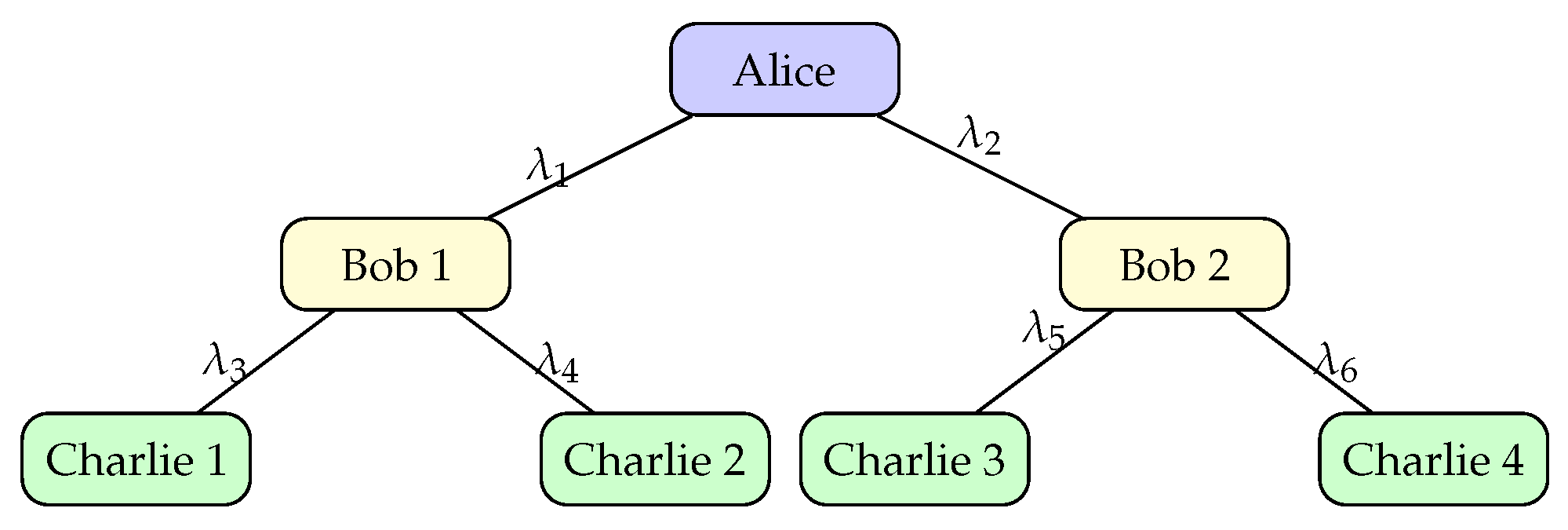
Haddadi et al. [38] studied the thermal evolution of the entropic uncertainty bound in the presence of quantum memory for an inhomogeneous, four-qubit, spin-star system and proved that the entropic uncertainty bound can be controlled and suppressed by adjusting the inhomogeneity parameter of the system. Related research on spin-star systems can be found in [39,40] and the references therein. As a generalization of star-networks [22,23], Yang et al. [41] considered the nonlocality of $(2^n-1)$-partite tree-tensor networks (referring to Figure 1 for the case where $n=2$) and derived the Bell-type inequalities.

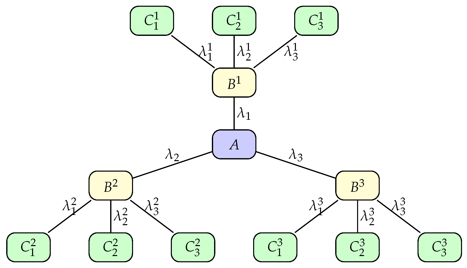
Extending the scenario in [41], Yang et al. [42] discussed the nonlocality of a type of multi-star-shaped QNs (Figure 2), called 3-layer m-star QNs (3-m-SQNWs), and established related Bell-type inequalities.

In this work, we study the nonlocality of star-shaped CTs and star-shaped PTs based on a more general multi-star network $MSN(m,n_1,\dots ,n_m)$ depicted in Figure 3.

Such a network consists of $1+m+n_1+\cdots +n_m$ nodes and one center-node A that connects to m star-nodes $B^1,B^2,\dots ,B^m$ while each star-node $B^j$ has $n_j+1$ star-nodes $A,C_1^j,C_2^j,\dots ,C_{n_j}^j$.

In Section 2, we will introduce the star-locality and star-nonlocality of the multi-star-network $MSN(m,n_1,\dots ,n_m)$ and give some related properties. In Section 3, we will first introduce star-shaped CTs (SSCTs), including star-shaped PTs (SSPTs), and discuss two types of localities of SSCTs and SSPTs, called D-star-locality and C-star-locality. Then, we establish a series of characterizations of D-star-localities and C-star-localities, show the equivalence of these two types of localities, and give some necessary conditions for star-shaped CT to be D-star-local. At the end of this section, we will show that the set ${\mathcal{CT}}^{\mathrm{star}-\mathrm{local}}({\mathrm{\Delta }}_S)$ of all star-local SSCTs over the index set ${\mathrm{\Delta }}_S$ is a compact and path-connected subset in the Hilbert space ${\mathcal{T}}^{\mathrm{star}}({\mathrm{\Delta }}_S)$ of all tensors over ${\mathrm{\Delta }}_S$ and contains at least two types of subsets that are star-convex. In Section 4, we shall establish an inequality that holds for all star-local SSCTs, called a star-Bell inequality. Based on our inequality, two examples are given. The first example is a star-nonlocal $MSN(m,n_1,\dots ,n_m)$, in which the shared states are all entangled pure states, and the second one gives a star-nonlocal $MSN(m,n_1,\dots ,n_m)$ in which the shared states are all entangled mixed states. In Section 5, we will give a summary and conclusions.

2. Multi-Star-Network Scenario

2.1. Notations and Concepts

In what follows, we consider the multi-star-network scenario as depicted in Figure 3, denoted by $MSN(m,n_1,\dots ,n_m)$. The network involves $1+m+{\sum }_{j=1}^m{n}_j$ parties

$$A,B^1,\dots ,B^m,C_1^1,\dots ,C_{n_1}^1,\dots ,C_1^m,\dots ,C_{n_m}^m$$

and $m+{\sum }_{j=1}^m{n}_j$ sources

$$S^1,\dots ,S^m,S_1^1,\dots ,S_{n_1}^1,\dots ,S_1^m,\dots ,S_{n_m}^m,$$

which are characterized by hidden variables ${\lambda }^j\in D_j$ and ${\mu }_k^j\in F_j(k)(j\in [m],k\in [n_j]$), where $[n]:=\{1,2,\dots ,n\}$.

We use ${\rho }_{A_j{B}_0^j}\in \mathcal{D}({\mathcal{H}}_{A^j}\otimes {\mathcal{H}}_{B_0^j})$ to denote the states shared by A and $B^j$ for all $j\in [m]$, and ${\rho }_{B_k^j{C}_k^j}\in \mathcal{D}({\mathcal{H}}_{B_k^j}\otimes {\mathcal{H}}_{C_k^j})$ to denote the states shared by $B^j$ and $C_k^j$ for all $j\in [m]$ and $k\in [n_j]$. We get ${\mathcal{H}}_A={⨂}_{j=1}^m{\mathcal{H}}_{A^j}$, ${\mathcal{H}}_{B^j}={\mathcal{H}}_{B_0^j}\otimes ({⨂}_{k=1}^{n_j}{\mathcal{H}}_{B_k^j})(j=1,2,\dots ,m)$. Then we define the system state as

$$\mathrm{\Gamma }=\left(\underset{j=1}{\overset{m}{⨂}}{\rho }_{A^j{B}_0^j}\right)\otimes \left(\underset{j=1}{\overset{m}{⨂}}({\rho }_{B_1^j{C}_1^j}\otimes {\rho }_{B_2^j{C}_2^j}\otimes \dots \otimes {\rho }_{B_{n_j}^j{C}_{n_j}^j})\right).$$

(1)

Consider the measurement assemblages

$$\left.\begin{array}{c}\mathcal{M}(A)=\left\{M(x):={\{M_{a|x}\}}_{a=1}^{o(A)}:x=1,2,\dots ,m(A)\right\},\hfill \\ \mathcal{N}(B^j)=\left\{N^j(y_j):={\{N_{b_j|y_j}^j\}}_{b_j=1}^{o(B^j)}:y_j=1,2,\dots ,m(B^j)\right\},\hfill \\ \mathcal{L}(C_k^j)=\left\{L_k^j(z_{j,k}):={\{L_{c_{j,k}|z_{j,k}}^{j,k}\}}_{c_{j,k}=1}^{o(C_k^j)}:z_{j,k}=1,2,\dots ,m(C_k^j)\right\}\hfill \end{array}\right\}$$

(2)

consisting of positive-operator-valued measures (POVMs), on systems A, $B^j$ and $C_k^j$, respectively, where $j\in [m]$ and $k\in [n_j]$, consisting of positive operators satisfying the normalization conditions:

$$\begin{array}{c}\hfill \sum _{a=1}^{o(A)}{M}_{a|x}=I_A,\sum _{b_j=1}^{o(B^j)}{N}_{b_j|y_j}^j=I_{B^j},\sum _{c_{j,k}=1}^{o(C_k^j)}{L}_{c_{j,k}|z_{j,k}}^{j,k}=I_{C_k^j}.\end{array}$$

Then, we can obtain a measurement assemblage (MA)

$$\begin{array}{c}\hfill \mathcal{M}:=\mathcal{M}(A)\otimes \left(\underset{j=1}{\overset{m}{⨂}}\mathcal{N}(B^j)\right)\otimes \left(\underset{j=1}{\overset{m}{⨂}}(\mathcal{L}(C_1^j)\otimes \mathcal{L}(C_2^j)\otimes \dots \otimes \mathcal{L}(C_{n_j}^j))\right)\end{array}$$

(3)

of the quantum network with measurement operators

$$\begin{array}{c}\hfill M_{a\mathbf{b}\mathbf{c}|x\mathbf{y}\mathbf{z}}:=M_{a|x}\otimes \left(\underset{j=1}{\overset{m}{⨂}}{N}_{b_j|y_j}^j\right)\otimes \left(\underset{j=1}{\overset{m}{⨂}}(L_{c_{j,1}|z_{j,1}}^{j,1}\otimes L_{c_{j,2}|z_{j,2}}^{j,2}\otimes \dots \otimes L_{c_{j,n_j}|z_{j,n_j}}^{j,n_j})\right),\end{array}$$

(4)

where $x\in [m(A)]$, $y_j\in [m(B^j)]$ and $z_k^j\in [m(C_k^j)]$ denote the inputs of parties A, $B^j$ and $C_k^j$ with the corresponding outputs $a\in [o(A)],b_j\in [o(B_j)]$ and $c_k^j\in [o(C_k^j)]$, respectively, and

$$\mathbf{y}=(y_1,y_2,\dots ,y_m)\equiv {\{y_j\}}_{j=1}^m,\mathbf{b}=(b_1,b_2,\dots ,b_m)\equiv {\{b_j\}}_{j=1}^m,$$

$$\mathbf{z}=(z_{1,1},\dots ,z_{1,n_1},z_{2,1},\dots ,z_{2,n_2},\dots ,z_{m,1},\dots ,z_{m,n_m})\equiv {\{z_{j,k}\}}_{j\in [m],k\in [n_j]},$$

$$\mathbf{c}=(c_{1,1},\dots ,c_{1,n_1},c_{2,1},\dots ,c_{2,n_2},\dots ,c_{m,1},\dots ,c_{m,n_m})\equiv {\{c_{j,k}\}}_{j\in [m],k\in [n_j]}.$$

Clearly, the measurement operators $M_{abc|xyz}$ are positive operators acting on the Hilbert space

$${\mathcal{H}}_{\mathrm{MHS}}:={\mathcal{H}}_A\otimes \left(\underset{j=1}{\overset{m}{⨂}}{\mathcal{H}}_{B^j}\right)\otimes \left(\underset{j=1}{\overset{m}{⨂}}({\mathcal{H}}_{C_1^j}\otimes {\mathcal{H}}_{C_2^j}\otimes \dots \otimes {\mathcal{H}}_{C_{n_j}^j})\right),$$

while the system state $\mathrm{\Gamma }$ given by (1) is an operator acting on the Hilbert space

$${\mathcal{H}}_{\mathrm{SHS}}:=\left(\underset{j=1}{\overset{m}{⨂}}({\mathcal{H}}_{A_j}\otimes {\mathcal{H}}_{B_0^j})\right)\otimes \left(\underset{j=1}{\overset{m}{⨂}}({\mathcal{H}}_{B_1^j}\otimes {\mathcal{H}}_{C_1^j}\otimes \dots \otimes {\mathcal{H}}_{B_{n_j}^j}\otimes {\mathcal{H}}_{C_{n_j}^j})\right).$$

Generally, ${\mathcal{H}}_{\mathrm{MHS}}\ne {\mathcal{H}}_{\mathrm{SHS}}$ due to the non-commutativity of tensor product, and in that case, the product $M_{a\mathbf{b}\mathbf{c}|x\mathbf{y}\mathbf{z}}\mathrm{\Gamma }$ does not work well. Therefore, we have to change the system state $\mathrm{\Gamma }$ to a state $\tilde{\mathrm{\Gamma }}$ acting on the space ${\mathcal{H}}_{\mathrm{MHS}}$ in order to make the tensor product $M_{a\mathbf{b}\mathbf{c}|x\mathbf{y}\mathbf{z}}\tilde{\mathrm{\Gamma }}$ reasonable. To do this, we define a swapping operation $U:{\mathcal{H}}_{\mathrm{SHS}}\to {\mathcal{H}}_{\mathrm{MHS}}$ by $|\mathrm{\Psi }\rangle \mapsto U|\mathrm{\Psi }\rangle$, where

$$\begin{array}{ccc}\hfill U|\mathrm{\Psi }\rangle & =& \left(\underset{j=1}{\overset{m}{⨂}}|{\psi }_{A_j}\rangle \right)\otimes \left(\underset{j=1}{\overset{m}{⨂}}(|{\psi }_{B_0^j}\rangle \otimes |{\psi }_{B_1^j}\rangle \otimes \dots \otimes |{\psi }_{B_m^j}\rangle )\right)\otimes \hfill \\ & & \left(\underset{j=1}{\overset{m}{⨂}}(|{\psi }_{C_1^j}\rangle \otimes \dots \otimes |{\psi }_{C_{n_j}^j}\rangle )\right)\hfill \\ & & \in {\mathcal{H}}_{\mathrm{MHS}}\hfill \end{array}$$

for all

$$\begin{array}{ccc}\hfill |\mathrm{\Psi }\rangle & =& \left(\underset{j=1}{\overset{m}{⨂}}\left(|{\psi }_{A_j}\rangle \otimes |{\psi }_{B_0^j}\rangle \right)\right)\hfill \\ & & \otimes \left(\underset{j=1}{\overset{m}{⨂}}\left(|{\psi }_{B_1^j}\rangle \otimes |{\psi }_{C_1^j}\rangle \otimes \dots \otimes |{\psi }_{B_{n_j}^j}\rangle \otimes |{\psi }_{C_{n_j}^j}\rangle \right)\right)\hfill \\ & & \in {\mathcal{H}}_{\mathrm{SHS}}.\hfill \end{array}$$

Then, we obtain a new state $\tilde{\mathrm{\Gamma }}=U\mathrm{\Gamma }{U}^{†}$ acting the Hilbert space ${\mathcal{H}}_{\mathrm{MHS}}$ so that the operator product $M_{a\mathbf{b}\mathbf{c}|x\mathbf{y}\mathbf{z}}\tilde{\mathrm{\Gamma }}$ works well. Furthermore, it is easy to see that

$$\mathrm{tr}[M_{a\mathbf{b}\mathbf{c}|x\mathbf{y}\mathbf{z}}\tilde{\mathrm{\Gamma }}]=\mathrm{tr}[{\tilde{M}}_{abc|xyz}\mathrm{\Gamma }],$$

(5)

where ${\tilde{M}}_{a\mathbf{b}\mathbf{c}|x\mathbf{y}\mathbf{z}}=U^{†}{M}_{a\mathbf{b}\mathbf{c}|x\mathbf{y}\mathbf{z}}U,$ which is an operator acting on the Hilbert space ${\mathcal{H}}_{\mathrm{SHS}}$ for every index $(a,\mathbf{b},\mathbf{c},x,\mathbf{y},\mathbf{z})$. Thus, the joint probability distribution $P(abc|xyz)$ of obtaining $a,b,c$ reads:

$$P_{\mathcal{M}}^{\mathrm{\Gamma }}(a\mathbf{b}\mathbf{c}|x\mathbf{y}\mathbf{z}):=\mathrm{tr}[M_{a\mathbf{b}\mathbf{c}|x\mathbf{y}\mathbf{z}}\tilde{\mathrm{\Gamma }}]=\mathrm{tr}[{\tilde{M}}_{a\mathbf{b}\mathbf{c}|x\mathbf{y}\mathbf{z}}\mathrm{\Gamma }].$$

(6)

With these preparations, we can describe the locality and nonlocality of our quantum network $MSN(m,n_1,\dots ,n_m)$ as follows.

Definition 1. 

A quantum network $MSN(m,n_1,\dots ,n_m)$ with the state (1) is said to be star-local for an MA $\mathcal{M}$ given by (3) if there exists a probability distribution (PD)

$$\begin{array}{c}\hfill p(\lambda ,{\mu }_1,\dots ,{\mu }_m)=\prod _{j=1}^{m}p({\lambda }^j)\times \prod _{j=1}^m\prod _{k=1}^{n_j}p({\mu }_k^j),\end{array}$$

(7)

where ${\{p_j({\lambda }^j)\}}_{{\lambda }^j}$ and ${\{p_{j,k}({\mu }_k^j)\}}_{{\mu }_k^j}$ are respectively probability distributions (PDs) of ${\lambda }^j$ and ${\mu }_k^j$ such that for all $a,\mathbf{b},\mathbf{c},x,\mathbf{y},\mathbf{z}$, it holds that

$$\begin{array}{ccc}\hfill P_{\mathcal{M}}^{\mathrm{\Gamma }}(a\mathbf{b}\mathbf{c}|x\mathbf{y}\mathbf{z})& =& \sum _{\lambda \in D,{\mu }_1\in F_1,\dots ,{\mu }_m\in F_m}p(\lambda ,{\mu }_1,\dots ,{\mu }_m)P_A(a|x,\lambda )\hfill \\ & & \times \prod _{j=1}^m{P}_{B^j}(b_j|y_j,{\lambda }^j,{\mu }_j)\times \prod _{j=1}^m\prod _{k=1}^{n_j}{P}_{C_k^j}(c_{j,k}|z_{j,k},{\mu }_k^j),\hfill \end{array}$$

(8)

where

$$\lambda =({\lambda }^1,\dots ,{\lambda }^m)\in D,{\mu }_j=({\mu }_1^j,\dots ,{\mu }_{n_j}^j)\in F_j(j\in [m])(\mathrm{local}\mathrm{hidden}\mathrm{variables}(\mathrm{LHVs}));$$

$$D=D_1\times \dots \times D_m,F_j=F_1^j\times \dots \times F_{n_j}^j(j\in [m])(\mathrm{finite}\mathrm{sets}\mathrm{of}\mathrm{LHVs}),$$

$\{P_A(a|x,\lambda )\},\{P_{B^j}(b_j|y_j,{\lambda }^j,{\mu }_j)\}$ and $\{P_{C_k^j}(c_{j,k}|z_{j,k},{\mu }_k^j)\}$ are PDs of $a,b_j$ and $c_{j,k}$, respectively. Otherwise, $MSN(m,n_1,\dots ,n_m)$ is said to be star-nonlocal for $\mathcal{M}$.

$MSN(m,n_1,\dots ,n_m)$ is said to be star-local if it is star-local for any $\mathcal{M}$, and it is said to be star-nonlocal if it is not star-local, i.e., it is star-nonlocal for some $\mathcal{M}$.

2.2. Properties

Similar to the reference [42], we can obtain the following results:

Proposition 1. 

If a network $MSN(m,n_1,\dots ,n_m)$ with the state (1) is star-local for $\mathcal{M}$ given by Equation (3), then the $\tilde{\mathrm{\Gamma }}$ as a state of system $A{B}_1\cdots B_m{C}_1^1\cdots C_{n_1}^1\cdots C_1^m\cdots C_{n_m}^m$ is Bell-local for $\mathcal{M}$.

Proposition 2. 

The reduced states of $\tilde{\mathrm{\Gamma }}$ on subsystems $A_j{B}_0^j$ and $B_k^j{C}_k^j$ are ${\tilde{\mathrm{\Gamma }}}_{A_j{B}_0^j}={\rho }_{A_j{B}_0^j}$ and ${\tilde{\mathrm{\Gamma }}}_{B_k^j{C}_k^j}={\rho }_{B_k^j{C}_k^j},$ respectively, for all $j\in [m]$ and $k\in [n_j]$.

Proposition 3. 

If the network $MSN(m,n_1,\dots ,n_m)$ with the state (1) is star-local, then the bipartite states ${\rho }_{B_t^j{C}_t^j}$ and ${\rho }_{A_j{B}_0^j}$ are Bell-local for all $s\in [m]$ and $t\in [n_j]$. Furthermore, the m-partite reduced state ${(\tilde{\mathrm{\Gamma }})}_{B^1{B}^2\dots B^m}$ is Bell-local.

Consequently, if one of bipartite states ${\rho }_{B_t^j{C}_t^j}$ and ${\rho }_{A_j{B}_0^j}$ is Bell-nonlocal, then the network $MSN(m,n_1,\dots ,n_m)$ must be star-nonlocal. Especially, if one of the shared states is a pure entangled state, then the network $MSN(m,n_1,\dots ,n_m)$ is star-nonlocal. See Examples 1 and 2 in Section 4.

Proposition 4. 

Every separable (i.e., all of the shared states are separable) $MSN(m,n_1,\dots ,n_m)$ is star-local.

Proof. 

Since the shared states ${\rho }_{A_j{B}_0^j}$ and ${\rho }_{B_k^j{C}_k^j}$ are separable, they can be written as

$${\rho }_{A_j{B}_0^j}=\sum _{{\lambda }^j=1}^{d_j}{p}_j({\lambda }^j)|s_{{\lambda }^j}^{\prime }\rangle \langle s_{{\lambda }^j}^{\prime }|\otimes |s_{{\lambda }^j}^{″}\rangle \langle s_{{\lambda }^j}^{″}|,$$

$${\rho }_{B_k^j{C}_k^j}=\sum _{{\mu }_k^j=1}^{d_k^j}{p}_{j,k}({\mu }_k^j)|t_{{\mu }_k^j}^{\prime }\rangle \langle t_{{\mu }_k^j}^{\prime }|\otimes |t_{{\mu }_k^j}^{″}\rangle \langle t_{{\mu }_k^j}^{″}|,$$

where $p_j({\lambda }^j)$ and $p_{j,k}({\mu }_k^j)$ are PDs of ${\lambda }^j$ and ${\mu }_k^j$. Put

$$\lambda =({\lambda }^1,{\lambda }^2,\dots ,{\lambda }^m),{\mu }_j=({\mu }_1^j,{\mu }_2^j,\dots ,{\mu }_{n_j}^j),$$

$$D=[d_1]\times \dots \times [d_m],F_j=[d_1^j]\times \dots \times [d_{n_j}^j](j\in [m]),$$

then

$$\begin{array}{ccc}\hfill \mathrm{\Gamma }& =& \left(\underset{j=1}{\overset{m}{⨂}}{\rho }_{A^j{B}_0^j}\right)\otimes \left(\underset{j=1}{\overset{m}{⨂}}({\rho }_{B_1^j{C}_1^j}\otimes {\rho }_{B_2^j{C}_2^j}\otimes \dots \otimes {\rho }_{B_{n_j}^j{C}_{n_j}^j})\right)\hfill \\ & =& \sum _{\lambda \in D}\sum _{{\mu }_1\in F_1,\dots ,{\mu }_m\in F_m}\prod _{j=1}^m{p}_j({\lambda }^j)\times \prod _{j=1}^m\prod _{k=1}^{n_j}{p}_{j,k}({\mu }_k^j)\hfill \\ & & \underset{j=1}{\overset{m}{⨂}}\left(|s_{{\lambda }^j}^{\prime }\rangle \langle s_{{\lambda }^j}^{\prime }|\otimes |s_{{\lambda }^j}^{″}\rangle \langle s_{{\lambda }^j}^{″}|\right)\otimes \left(\underset{j=1}{\overset{m}{⨂}}\underset{k=1}{\overset{n_j}{⨂}}|t_{{\mu }_k^j}^{\prime }\rangle \langle t_{{\mu }_k^j}^{\prime }|\otimes |t_{{\mu }_k^j}^{″}\rangle \langle t_{{\mu }_k^j}^{″}|\right),\hfill \end{array}$$

which induces the measurement state

$$\begin{array}{c}\hfill \tilde{\mathrm{\Gamma }}=U\mathrm{\Gamma }{U}^{†}=\sum _{\lambda \in D}\sum _{{\mu }_1\in F_1,\dots ,{\mu }_m\in F_m}\prod _{j=1}^m{p}_j({\lambda }^j)\times \prod _{j=1}^m\prod _{k=1}^{n_j}{p}_{j,k}({\mu }_k^j)\times {\mathrm{\Gamma }}^{\prime }(\lambda ,{\mu }_1,\dots ,{\mu }_m),\end{array}$$

where

$$\begin{array}{ccc}\hfill {\mathrm{\Gamma }}^{\prime }(\lambda ,{\mu }_1,\dots ,{\mu }_m)& =& \left(\underset{j=1}{\overset{m}{⨂}}|s_{{\lambda }^j}^{\prime }\rangle \langle s_{{\lambda }^j}^{\prime }|\right)\otimes \left(\underset{j=1}{\overset{m}{⨂}}\left(|s_{{\lambda }^j}^{″}\rangle \langle s_{{\lambda }^j}^{″}|\otimes \underset{k=1}{\overset{n_j}{⨂}}|t_{{\mu }_k^j}^{\prime }\rangle \langle t_{{\mu }_k^j}^{\prime }|\right)\right)\hfill \\ & & \otimes \left(\underset{j=1}{\overset{m}{⨂}}\underset{k=1}{\overset{n_j}{⨂}}|t_{{\mu }_k^j}^{″}\rangle \langle t_{{\mu }_k^j}^{″}|\right).\hfill \end{array}$$

Thus, for any MA $\mathcal{M}$ given by (3), we compute that

$$\begin{array}{ccc}\hfill P_{\mathcal{M}}^{\mathrm{\Gamma }}(a\mathbf{b}\mathbf{c}|x\mathbf{y}\mathbf{z})& =& \mathrm{tr}[(M_{a\mid x}\otimes N_{\mathbf{b}\mid \mathbf{y}}\otimes L_{\mathbf{c}\mid \mathbf{z}})\tilde{\mathrm{\Gamma }}]\hfill \\ & =& \sum _{\lambda \in D}\sum _{{\mu }_1\in F_1,\dots ,{\mu }_m\in F_m}\prod _{j=1}^m{p}_j({\lambda }^j)\times \prod _{j=1}^m\prod _{k=1}^{n_j}{p}_{j,k}({\mu }_k^j)\hfill \\ & & \times \mathrm{tr}[(M_{a\mid x}\otimes N_{\mathbf{b}\mid \mathbf{y}}\otimes L_{\mathbf{c}\mid \mathbf{z}}){\mathrm{\Gamma }}^{\prime }(\lambda ,{\mu }_1,\dots ,{\mu }_m)]\hfill \\ & =& \sum _{\lambda \in D,{\mu }_1\in F_1,\dots ,{\mu }_m\in F_m}\prod _{j=1}^m{p}_j({\lambda }^j)\times \prod _{j=1}^m\prod _{k=1}^{n_j}{p}_{j,k}({\mu }_k^j)\times P_A(a|x,\lambda )\hfill \\ & & \times \prod _{j=1}^m{P}_{B^j}(b_j|y_j,{\lambda }^j,{\mu }_j)\times \prod _{j=1}^m\prod _{k=1}^{n_j}{P}_{C_k^j}(c_{j,k}|z_{j,k},{\mu }_k^j),\hfill \end{array}$$

(9)

where

$$P_A(a|x,\lambda )=\mathrm{tr}[M_{a|x}\left(\underset{j=1}{\overset{m}{⨂}}|s_{{\lambda }^j}^{\prime }\rangle \langle s_{{\lambda }^j}^{\prime }|\right)];$$

$$P_{B^j}(b_j|y_j,{\lambda }^j,{\mu }_j)=\mathrm{tr}[N_{b_j|y_j}(|s_{{\lambda }^j}^{″}\rangle \langle s_{{\lambda }^j}^{″}|\otimes \underset{k=1}{\overset{n_j}{⨂}}|t_{{\mu }_k^j}^{\prime }\rangle \langle t_{{\mu }_k^j}^{\prime }|)];$$

$$P_{C_k^j}(c_{j,k}|z_{j,k},{\mu }_k^j)=\mathrm{tr}[L_{c_k^j|z_k^j}|t_{{\mu }_k^j}^{″}\rangle \langle t_{{\mu }_k^j}^{″}|)].$$

This shows that Equation (8) holds and then the network is star-local. The proof is completed. □

3. Star-Locality of Star-Shaped Cts

When a multi-star network given by Figure 3 for the case that $m=3$ is measured by parties

$$A,B^1,\dots ,B^m,C_1^1,\dots ,C_{n_1}^1,\dots ,C_1^m,\dots ,C_{n_m}^m,$$

the conditional probabilities $P(a\mathbf{b}\mathbf{c}|x\mathbf{y}\mathbf{z})$ of obtaining result $(a,\mathbf{b},\mathbf{c})$ conditioned on the measurement choice $(x,\mathbf{y},\mathbf{z})$ form a correlation tensor (CT) [44] $\mathbf{P}=〚P(a\mathbf{b}\mathbf{c}|x\mathbf{y}\mathbf{z})〛$ over the index set

$$\begin{array}{c}\hfill {\mathrm{\Delta }}_S=[o(A)]\times \prod _{j=1}^m[o(B^j)]\times \prod _{j=1}^m\prod _{k=1}^{n_j}[o(C_k^j)]\times [m_A]\times \prod _{j=1}^m[m(B^j)]\times \prod _{j=1}^m\prod _{k=1}^{n_j}[m(C_k^j)],\end{array}$$

(10)

which is a non-negative function defined on ${\mathrm{\Delta }}_S$ satisfying the following completeness condition:

$$\sum _{a,\mathbf{b},\mathbf{c}}P(a\mathbf{b}\mathbf{c}|x\mathbf{y}\mathbf{z})=1,\forall x,\mathbf{y},\mathbf{z}.$$

(11)

We call such a $\mathbf{P}$ a star-shaped CT over ${\mathrm{\Delta }}_S$. Let ${\mathcal{CT}}^{\mathrm{star}}({\mathrm{\Delta }}_S)$ be the set of all star-shaped CTs over ${\mathrm{\Delta }}_S$.

To discuss the algebraic and topological properties of the ${\mathcal{CT}}^{\mathrm{star}}({\mathrm{\Delta }}_S)$, we have to make it live in a Hilbert space. To accomplish this, we let ${\mathcal{T}}^{\mathrm{star}}({\mathrm{\Delta }}_S)$ be the set of all real tensors $\mathbf{P}=〚P(a\mathbf{b}\mathbf{c}|x\mathbf{y}\mathbf{z})〛$ over ${\mathrm{\Delta }}_S$. That is, $\mathbf{P}\in {\mathcal{T}}^{\mathrm{star}}({\mathrm{\Delta }}_S)$ if and only if it is a real-valued function defined on ${\mathrm{\Delta }}_S$ with the value $P(a\mathbf{b}\mathbf{c}|x\mathbf{y}\mathbf{z})$ and a point $(a,\mathbf{b},\mathbf{c},x,\mathbf{y},\mathbf{z})$ in ${\mathrm{\Delta }}_S$. Clearly, ${\mathcal{T}}^{\mathrm{star}}({\mathrm{\Delta }}_S)$ becomes a finite-dimensional Hilbert space over $\mathbb{R}$ with respect to the following operation and inner product:

$$s{\mathbf{P}}_1+t{\mathbf{P}}_2=〚s{P}_1(a\mathbf{b}\mathbf{c}|x\mathbf{y}\mathbf{z})+t{P}_2(a\mathbf{b}\mathbf{c}|x\mathbf{y}\mathbf{z})〛,$$

$$\langle {\mathbf{P}}_1,{\mathbf{P}}_2\rangle =\sum _{a,\mathbf{b},\mathbf{c},x,\mathbf{y},\mathbf{z}}{P}_1(a\mathbf{b}\mathbf{c}|x\mathbf{y}\mathbf{z})P_2(a\mathbf{b}\mathbf{c}|x\mathbf{y}\mathbf{z}).$$

The norm induced by the inner product reads

$$\parallel \mathbf{P}\parallel :=\sqrt{\langle \mathbf{P},\mathbf{P}\rangle }={\left\{\sum _{a,\mathbf{b},\mathbf{c},x,\mathbf{y},\mathbf{z}}{(P(a\mathbf{b}\mathbf{c}|x\mathbf{y}\mathbf{z}))}^2\right\}}^{\frac{1}{2}}.$$

Especially, when $m(A)=m(B^j)=m(C_k^j)=1$ for all $k,j$, we denote $\mathbf{P}=〚P(a\mathbf{b}\mathbf{c}|x\mathbf{y}\mathbf{z})〛$ by $\mathbf{P}=〚P(a\mathbf{b}\mathbf{c})〛$ and call it a star-shaped probability tensor (PT) over

$${\mathrm{\Omega }}_S=[o(A)]\times \prod _{j=1}^m[o(B^j)]\times \prod _{j=1}^m\prod _{k=1}^{n_j}[o(C_k^j)].$$

Let ${\mathcal{PT}}^{\mathrm{star}}({\mathrm{\Omega }}_S)$ be the set of all star-shaped PTs over ${\mathrm{\Omega }}_S$ and let ${\mathcal{T}}^{\mathrm{star}}({\mathrm{\Omega }}_S)$ be the set of all real tensors $\mathbf{P}=〚P(a\mathbf{b}\mathbf{c})〛$ over ${\mathrm{\Omega }}_S$, which is a finite-dimensional Hilbert space over $\mathbb{R}$ with respect to the following operation and inner product:

$$s{\mathbf{P}}_1+t{\mathbf{P}}_2=〚s{P}_1(a\mathbf{b}\mathbf{c})+t{P}_2(a\mathbf{b}\mathbf{c})〛,$$

$$\langle {\mathbf{P}}_1,{\mathbf{P}}_2\rangle =\sum _{a,\mathbf{b},\mathbf{c}}{P}_1(a\mathbf{b}\mathbf{c})P_2(a\mathbf{b}\mathbf{c}).$$

The norm induced by the inner product reads

$$\parallel \mathbf{P}\parallel :=\sqrt{\langle \mathbf{P},\mathbf{P}\rangle }={\left\{\sum _{a,\mathbf{b},\mathbf{c}}{(P(a\mathbf{b}\mathbf{c}))}^2\right\}}^{\frac{1}{2}}.$$

3.1. Concepts

Definition 2. 

A star-shaped CT $\mathbf{P}=〚P(a\mathbf{b}\mathbf{c}|x\mathbf{y}\mathbf{z})〛$ over ${\mathrm{\Delta }}_S$ is said to be C-star-local if it admits a “C-star-shaped LHVM":

$$\begin{array}{ccc}\hfill P(a\mathbf{b}\mathbf{c}|x\mathbf{y}\mathbf{z})& =& {\int }_{D\times F_1\times \dots \times F_m}p(\lambda ,{\mu }_1,\dots ,{\mu }_m)P_A(a|x,\lambda )\prod _{j=1}^m{P}_{B^j}(b_j|y_j,{\lambda }^j,{\mu }_j)\hfill \\ & & \times \prod _{j=1}^m\prod _{k=1}^{n_j}{P}_{C_k^j}(c_{j,k}|z_{j,k},{\mu }_k^j)\mathrm{d}\gamma (\lambda )\mathrm{d}{\tau }_1({\mu }_1)\dots \mathrm{d}{\tau }_m({\mu }_m)\hfill \end{array}$$

(12)

for all $a,\mathbf{b},\mathbf{c},x,\mathbf{y},\mathbf{z}$, where

(i) $(\mathrm{\Lambda },\mathrm{\Omega },\mu )\equiv \left(D\times {\prod }_{j=1}^m{F}_j,\sigma \times {\prod }_{j=1}^m{\delta }_j,\gamma \times {\prod }_{j=1}^m{\tau }_j\right)$ is a product measure space with

$$\lambda =({\lambda }^1,\dots ,{\lambda }^m)\in D,{\mu }_j=({\mu }_1^j,\dots ,{\mu }_{n_j}^j)\in F_j(j\in [m])(\mathrm{LHVs});$$

$$D=D_1\times \dots \times D_m,F_j=F_1^j\times \dots \times F_{n_j}^j(j\in [m])(\mathrm{spaces}\mathrm{of}\mathrm{LHVs});$$

$$\sigma =\prod _{j=1}^m{\sigma }_j,{\delta }_j=\prod _{k=1}^{n_j}{\delta }_k^j(j\in [m])(\mathrm{product}\sigma -\mathrm{algebras});$$

$$\gamma =\prod _{j=1}^m{\gamma }_j,{\tau }_j=\prod _{k=1}^{n_j}{\tau }_k^j(j\in [m])(\mathrm{product}\mathrm{measures});$$

(ii) All of the local hidden variables (LHVs) ${\lambda }^1,\dots ,{\lambda }^m,{\mu }_1^j,\dots ,{\mu }_{n_j}^j(\forall j\in [m])$ are independent, i.e.,

$$p(\lambda ,{\mu }_1,\dots ,{\mu }_m)=\prod _{j=1}^m{p}_j({\lambda }^j)\times \prod _{j=1}^m\prod _{k=1}^{n_j}{p}_{j,k}({\mu }_k^j),$$

(13)

where $p_j({\lambda }^j)$ and $p_{j,k}({\mu }_k^j)$ are density functions (DFs) of ${\lambda }_j$ and ${\mu }_k^j$, respectively, i.e., they are non-negative and satisfy

$${\int }_{D_j}{p}_j({\lambda }^j)\mathrm{d}{\gamma }_j({\lambda }^j)=1,{\int }_{F_k^j}{p}_{j,k}({\mu }_k^j)\mathrm{d}{\tau }_k^j({\mu }_k^j)=1;$$

(iii) $P_A(a|x,\lambda ),P_{B^j}(b_j|y_j,{\lambda }^j,{\mu }_j)$ and $P_{C_k^j}(c_{j,k}|z_{j,k},{\mu }_k^j)$ are PDs of $a,b_j$ and $c_{j,k}$, respectively, and are measurable with respect to $\lambda ,({\lambda }^j,{\mu }_j)$ and ${\mu }_k^j$, respectively.

A star-shaped CT $\mathbf{P}=〚P(a\mathbf{b}\mathbf{c}|x\mathbf{y}\mathbf{z})〛$ over ${\mathrm{\Delta }}_S$ is said to be C-star-nonlocal if it is not C-star-local.

We use ${\mathcal{CT}}^{\mathrm{C}-\mathrm{star}-\mathrm{local}}({\mathrm{\Delta }}_S)$ and ${\mathcal{CT}}^{\mathrm{C}-\mathrm{star}-\mathrm{nonlocal}}({\mathrm{\Delta }}_S)$ to denote the sets of all C-star-local CTs and all C-star-nonlocal CTs over ${\mathrm{\Delta }}_S$, respectively.

Specifically, when $D_1,\dots ,D_m,F_1^j,\dots ,F_{n_j}^j(j\in [m])$ are finite sets with the counting measures, a C-star-shaped-LHVM (12) becomes a “D-star-shaped-LHVM”:

$$\begin{array}{ccc}\hfill P(a\mathbf{b}\mathbf{c}|x\mathbf{y}\mathbf{z})& =& \sum _{\lambda \in D,{\mu }_1\in F_1,\dots ,{\mu }_m\in F_m}p(\lambda ,{\mu }_1,\dots ,{\mu }_m)P_A(a|x,\lambda )\hfill \\ & & \times \prod _{j=1}^m{P}_{B^j}(b_j|y_j,{\lambda }^j,{\mu }_j)\times \prod _{j=1}^m\prod _{k=1}^{n_j}{P}_{C_k^j}(c_{j,k}|z_{j,k},{\mu }_k^j),\hfill \end{array}$$

(14)

where $\{P_A(a|x,\lambda )\},\{P_{B^j}(b_j|y_j,{\lambda }^j,{\mu }_j)\}$, and $\{P_{C_k^j}(c_{j,k}|z_{j,k},{\mu }_k^j)\}$ are PDs of $a,b_j$ and $c_{j,k}$, respectively, and the joint PD $p(\lambda ,{\mu }_1,\dots ,{\mu }_m)$ is given by (13). In this case, we say that $\mathbf{P}$ is D-star-local. If $\mathbf{P}$ has no D-star-shaped LHVMs of the form (14), then we say that it is D-star-nonlocal.

We use ${\mathcal{CT}}^{\mathrm{D}-\mathrm{star}-\mathrm{local}}({\mathrm{\Delta }}_S)$ and ${\mathcal{CT}}^{\mathrm{D}-\mathrm{star}-\mathrm{nonlocal}}({\mathrm{\Delta }}_S)$ to denote the sets of all D-star-local CTs and all D-star-nonlocal CTs over ${\mathrm{\Delta }}_S$, respectively. Clearly,

$${\mathcal{CT}}^{\mathrm{D}-\mathrm{star}-\mathrm{local}}({\mathrm{\Delta }}_S)\subset {\mathcal{CT}}^{\mathrm{C}-\mathrm{star}-\mathrm{local}}({\mathrm{\Delta }}_S).$$

Definition 3. 

A star-shaped PT $\mathbf{P}=〚P(a\mathbf{b}\mathbf{c})〛$ over ${\mathrm{\Omega }}_S$ is said to be C-star-local if it admits a ”C-star-shaped LHVM”:

$$\begin{array}{ccc}\hfill P(a\mathbf{b}\mathbf{c})& =& {\int }_{D\times F_1\times \dots \times F_m}p(\lambda ,{\mu }_1,\dots ,{\mu }_m)P_A(a|\lambda )\prod _{j=1}^m{P}_{B^j}(b_j|{\lambda }^j,{\mu }_j)\hfill \\ & & \times \prod _{j=1}^m\prod _{k=1}^{n_j}{P}_{C_k^j}(c_{j,k}|{\mu }_k^j)\mathrm{d}\gamma (\lambda )\mathrm{d}{\tau }_1({\mu }_1)\dots \mathrm{d}{\tau }_m({\mu }_m)\hfill \end{array}$$

(15)

for all $a,\mathbf{b},\mathbf{c}$, where $p(\lambda ,{\mu }_1,\dots ,{\mu }_m)$ is a DF of the form (13). It is said to be C-star-nonlocal if it is not C-star-local.

Definition 4. 

A star-shaped PT $\mathbf{P}=〚P(a\mathbf{b}\mathbf{c})〛$ over ${\mathrm{\Omega }}_S$ is said to be D-star-local if it admits a ”D-star-shaped LHVM":

$$\begin{array}{ccc}\hfill P(a\mathbf{b}\mathbf{c})& =& \sum _{\lambda \in D,{\mu }_1\in F_1,\dots ,{\mu }_m\in F_m}p(\lambda ,{\mu }_1,\dots ,{\mu }_m)P_A(a|\lambda )\hfill \\ & & \times \prod _{j=1}^m{P}_{B^j}(b_j|{\lambda }^j,{\mu }_j)\times \prod _{j=1}^m\prod _{k=1}^{n_j}{P}_{C_k^j}(c_{j,k}|{\mu }_k^j)\hfill \end{array}$$

(16)

for all $a,\mathbf{b},\mathbf{c}$, where $p(\lambda ,{\mu }_1,\dots ,{\mu }_m)$ is a PD of the form (13). It is said to be D-star-nonlocal if it is not D-star-local.

Definition 5. 

A star-shaped PT $\mathbf{P}=〚P(a\mathbf{b}\mathbf{c})〛$ over ${\mathrm{\Omega }}_S$ is said to be star-local if it is either C-star-local or D-star-local. It is said to be star-nonlocal if is neither C-star-local nor D-star-local.

We use ${\mathcal{PT}}^{\mathrm{C}-\mathrm{star}-\mathrm{local}}({\mathrm{\Omega }}_S)$ (resp., ${\mathcal{PT}}^{\mathrm{D}-\mathrm{star}-\mathrm{local}}({\mathrm{\Omega }}_S)$) to denote the set of all C-star-local (resp., D-star-local) star-shaped PTs over ${\mathrm{\Omega }}_S$.

Clearly,

$${\mathcal{PT}}^{\mathrm{D}-\mathrm{star}-\mathrm{local}}({\mathrm{\Omega }}_S)\subset {\mathcal{PT}}^{\mathrm{C}-\mathrm{star}-\mathrm{local}}({\mathrm{\Omega }}_S).$$

3.2. Characterizations

To show every C-star-local CT (especially every PT) is D-star-local, we need the following lemma [37,43]. Recall that an $m\times n$ function matrix $B(\lambda )=[b_{ij}(\lambda )]$ on $\mathrm{\Lambda }$ is said to be row-statistic (RS) if, for each $\lambda \in \mathrm{\Lambda }$, $b_{ij}(\lambda )\ge 0$ for all $i,j$ and ${\sum }_{j=1}^n{b}_{ij}(\lambda )=1.$

Lemma 1. 

Let $(\mathrm{\Lambda },\mathrm{\Omega })$ be a measurable space and let $B(\lambda )=[b_{ij}(\lambda )]$ be an $m\times n$ RS function matrix whose entries $b_{ij}$ are Ω-measurable on Λ. Then, $B(\lambda )$ can be written as:

$$B(\lambda )=\sum _{k=1}^{n^m}{\alpha }_k(\lambda )[{\delta }_{j,J_k(i)}],\forall \lambda \in \mathrm{\Lambda },$$

(17)

where ${\alpha }_k(k=1,2,\dots ,n^m)$ are all non-negative and Ω-measurable functions on Λ with ${\sum }_{k=1}^{n^m}{\alpha }_k(\lambda )=1$ for all $\lambda \in \mathrm{\Lambda }$, and ${\{J_k\}}_{k=1}^{n^m}$ denotes the set of all maps from $[m]$ into $[n]$.

Put

$$N(A)=o{(A)}^{m(A)},N(B^j)=o{(B^j)}^{m(B^j)},N(C_k^j)=o{(C_k^j)}^{m(C_k^j)}$$

and let ${\{J_i\}}_{i=1}^{N(A)}$ be the set of all maps from $[m(A)]$ into $[o(A)]$, ${\{K_{s_j}^j\}}_{s_j=1}^{N(B^j)}$ the set of all maps from $[m(B^j)]$ into $[o(B^j)]$, and let ${\{L_{t_{jk}}^{j,k}\}}_{t_{jk}=1}^{N(C_k^j)}$ be the set of all maps from $[m(C_k^j)]$ into $[o(C_k^j)]$.

Let $\mathbf{P}=〚P(a\mathbf{b}\mathbf{c}|x\mathbf{y}\mathbf{z})〛$ be a C-star-local CT over ${\mathrm{\Delta }}_S$. Then, it has a C-star-shaped LHVM (12). Since function matrices

$$M(\lambda ):={[P_A(a\mid x,\lambda )]}_{x,a},M({\lambda }^j,{\mu }_j):={[P_{B^j}(b_j|y_j,{\lambda }^j,{\mu }_j)]}_{y_j,b_j},M({\mu }_k^j):={[P_{C_k^j}(c_{j,k}|z_{j,k},{\mu }_k^j)]}_{z_{j,k},c_{j,k}}$$

are RS for each parameters $\lambda ,({\lambda }^j,{\mu }_j),{\mu }_k^j$ and their entries are measurable with respect to the related parameters, respectively, it follows from Lemma 1 that they have the following decompositions:

$$M(\lambda )=\sum _{i=1}^{N(A)}\alpha (i|\lambda )[{\delta }_{a,J_i(x)}],$$

$$M({\lambda }^j,{\mu }_j)=\sum _{s_j=1}^{N(B^j)}{\beta }^j(s_j|{\lambda }^j,{\mu }_j)[{\delta }_{b_j,K_{s_j}^j(y_j)}],$$

$$M({\mu }_k^j)=\sum _{t_{jk}=1}^{N(C_k^j)}{f}^{j,k}(t_{jk}|{\mu }_k^j)[{\delta }_{c_{j,k},L_{t_{jk}}^{j,k}(z_{j,k})}];$$

equivalently,

$$P_A(a\mid x,\lambda )=\sum _{i=1}^{N(A)}\alpha (i|\lambda ){\delta }_{a,J_i(x)},$$

(18)

$$P_{B^j}(b_j|y_j,{\lambda }^j,{\mu }_j)=\sum _{s_j=1}^{N(B^j)}{\beta }^j(s_j|{\lambda }^j,{\mu }_j){\delta }_{b_j,K_{s_j}^j(y_j)},$$

(19)

$$P_{C_k^j}(c_{j,k}|z_{j,k},{\mu }_k^j)=\sum _{t_{jk}=1}^{N(C_k^j)}{f}^{j,k}(t_{jk}|{\mu }_k^j){\delta }_{c_{j,k},L_{t_{jk}}^{j,k}(z_{j,k})},$$

(20)

where ${\alpha }_i(\lambda )$, ${\beta }_{s_j}^j({\lambda }^j,{\mu }_j)$ and $f_{t_{jk}}^{j,k}({\mu }_k^j)$ are PDs of $i,s_j$ and $t_{jk}$, respectively, and are measurable with respect to $\lambda ,({\lambda }^j,{\mu }_j)$ and ${\mu }_k^j$, respectively. It follows from Equations (12) and (18)–(20) that

$$\begin{array}{c}\hfill P(a\mathbf{b}\mathbf{c}|x\mathbf{y}\mathbf{z})=\sum _{i,s_j,t_{jk}}\pi (i,\mathbf{s},\mathbf{t}){\delta }_{a,J_i(x)}\prod _{j=1}^m{\delta }_{b_j,K_{s_j}^j(y_j)}\times \prod _{j=1}^m\prod _{k=1}^{n_j}{\delta }_{c_{j,k},L_{t_{jk}}^{j,k}(z_{j,k})}\end{array}$$

(21)

for all $a,\mathbf{b},\mathbf{c},x,\mathbf{y},\mathbf{z}$, where $\mathbf{s}=(s_1,s_2,\dots ,s_m)\equiv {\{s_j\}}_{j=1}^m,$

$$\mathbf{t}=(t_{11},t_{12},\dots ,t_{1n_1},t_{21},t_{22},\dots ,t_{2n_2},\dots ,t_{m1},t_{m2},\dots ,t_{m{n}_m})\equiv {\{t_{jk}\}}_{j\in [m],k\in [n_j]},$$

and

$$\begin{array}{ccc}\hfill \pi (i,\mathbf{s},\mathbf{t})& =& {\int }_{D\times F_1\times \dots \times F_m}p(\lambda ,{\mu }_1,\dots ,{\mu }_m)\alpha (i|\lambda )\prod _{j=1}^m{\beta }^j(s_j|{\lambda }^j,{\mu }_j)\hfill \\ & & \times \prod _{j=1}^m\prod _{k=1}^{n_j}{f}^{j,k}(t_{jk}|{\mu }_k^j)\mathrm{d}\gamma (\lambda )\mathrm{d}{\tau }_1({\mu }_1)\dots \mathrm{d}{\tau }_m({\mu }_m),\hfill \end{array}$$

(22)

with $p(\lambda ,{\mu }_1,\dots ,{\mu }_m)$ given by (13). Clearly, $\mathbf{p}=〚\pi (i,\mathbf{s},\mathbf{t})〛$ is a C-star-local PT over

$${\mathrm{\Gamma }}_S=[N(A)]\times \prod _{j=1}^m[N(B^j)]\times \prod _{j=1}^m\prod _{k=1}^{n_i}[N(C_k^j)],$$

which generates $\mathbf{P}$ in terms of Equation (21).

Conversely, if (21) holds for some completely independent PD (13) and a C-star-local PT $\mathbf{p}=〚\pi (i,\mathbf{s},\mathbf{t})〛$ with a C-star-shaped LHVM (22), then (12) holds for $P_A,P_{B^j}$ and $P_{C_k^j}$ given by Equations (18)–(20). Thus, $\mathbf{P}$ is C-star-local.

This shows that (12) ⇔ (21) and leads to the following.

Theorem 1. 

A star-shaped CT $\mathbf{P}$ over ${\mathrm{\Delta }}_S$ is C-star-local if and only if it has the following decomposition:

$$\mathbf{P}=\sum _{i,\mathbf{s},\mathbf{t}}\pi (i,\mathbf{s},\mathbf{t}){\mathbf{D}}_{i,\mathbf{s},\mathbf{t}},$$

(23)

where $\mathbf{p}=〚\pi (i,\mathbf{s},\mathbf{t})〛$ is a C-star-local PT over ${\mathrm{\Gamma }}_S$ given by (22) and ${\mathbf{D}}_{i,\mathbf{s},\mathbf{t}}=〚D_{i,\mathbf{s},\mathbf{t}}(a\mathbf{b}\mathbf{c}|x\mathbf{y}\mathbf{z})〛$ is given by

$$D_{i,\mathbf{s},\mathbf{t}}(a\mathbf{b}\mathbf{c}|x\mathbf{y}\mathbf{z})={\delta }_{a,J_i(x)}\prod _{j=1}^m{\delta }_{b_j,K_{s_j}^j(y_j)}\times \prod _{j=1}^m\prod _{k=1}^{n_j}{\delta }_{c_{j,k},L_{t_{jk}}^{j,k}(z_{j,k})}.$$

As an application of Theorem 1, we obtain the following relationship between C-star-local CTs and C-star-local PTs:

$${\mathcal{CT}}^{\mathrm{C}-\mathrm{star}-\mathrm{local}}({\mathrm{\Delta }}_S)=\left\{\sum _{i,\mathbf{s},\mathbf{t}}\pi (i,\mathbf{s},\mathbf{t}){\mathbf{D}}_{i,\mathbf{s},\mathbf{t}}:\mathbf{p}=〚\pi (i,\mathbf{s},\mathbf{t})〛\in {\mathcal{PT}}^{\mathrm{C}-\mathrm{star}-\mathrm{local}}({\mathrm{\Gamma }}_S)\right\}$$

(24)

Again, we let $\mathbf{P}$ be a C-star-local CT over ${\mathrm{\Delta }}_S$. We aim to prove that $\mathbf{P}$ is D-star-local. First, it has a C-star-shaped LHVM (12). Since

$$p(\lambda ,{\mu }_1,\dots ,{\mu }_m)=\prod _{j=1}^m{p}_j({\lambda }^j)\times \prod _{j=1}^m\prod _{k=1}^{n_j}{p}_{j,k}({\mu }_k^j),$$

we obtain from (12) and (20) that

$$\begin{array}{ccc}\hfill P(a\mathbf{b}\mathbf{c}|x\mathbf{y}\mathbf{z})& =& \sum _{t_{jk}\in [N(C_{n_j}^j)](j\in [m])}{\int }_D\prod _{j=1}^m{p}_j({\lambda }^j)\times P_A(a|x,\lambda )\mathrm{d}\gamma (\lambda )\hfill \\ & & \times {\int }_{F_1\times \dots \times F_m}\prod _{j=1}^m{P}_{B^j}(b_j|y_j,{\lambda }^j,{\mu }_j)\times \prod _{j=1}^m\prod _{k=1}^{n_j}{p}_{j,k}({\mu }_k^j)f_{t_{jk}}^{j,k}({\mu }_k^j)\mathrm{d}{\tau }_1({\mu }_1)\dots \mathrm{d}{\tau }_m({\mu }_m)\hfill \\ & & \times \prod _{j=1}^m\prod _{k=1}^{n_j}{\delta }_{c_{j,k},L_{t_{jk}}^{j,k}(z_{j,k})}.\hfill \end{array}$$

(25)

Put

$$q_{j,k}(t_{jk})={\int }_{F_k^j}{f}_{t_{jk}}^{j,k}({\mu }_k^j)p_{j,k}({\mu }_k^j)\mathrm{d}{\tau }_k^j({\mu }_k^j),$$

which are PDs of $t_{jk}$ and satisfy

$$\prod _{k=1}^{n_j}{q}_{j,k}(t_{jk})={\int }_{F_j}\prod _{k=1}^{n_j}(f_{t_{jk}}^{j,k}({\mu }_k^j)p_{j,k}({\mu }_k^j))\mathrm{d}{\tau }_j({\mu }_j),$$

and define

$$\begin{array}{ccc}\hfill P_{B^j}(b_j\mid y_j,{\lambda }^j,t_{j1},\dots ,t_{j{n}_j})& =& \frac{1}{{\prod }_{k=1}^{n_j}{q}_{j,k}(t_{jk})}{\int }_{F_j}{P}_{B^j}(b_j|y_j,{\lambda }^j,{\mu }_j)\times \left(\prod _{k=1}^{n_j}{f}_{t_{jk}}^{j,k}({\mu }_k^j)p_{j,k}({\mu }_k^j)\right)\mathrm{d}{\tau }_j({\mu }^j)\hfill \end{array}$$

if ${\prod }_{k=1}^{n_j}{q}_{j,k}(t_{jk})>0$; and

$$P_{B^j}(b_j\mid y_j,{\lambda }^j,t_{j1},\dots ,t_{j{n}_j})=\frac{1}{o(B^j)},$$

otherwise. Clearly, $P_{B^j}(b_j\mid y_j,{\lambda }^j,t_{j1},\dots ,t_{j{n}_j})$ is a PD of $b_j$ for each $(y_j,{\lambda }^j,t_{j1},\dots ,t_{j{n}_j})$, and when ${\prod }_{k=1}^{n_j}{q}_{j,k}(t_{jk})>0$, we have

$$\begin{array}{c}\hfill \prod _{k=1}^{n_j}{q}_{j,k}(t_{jk})\times P_{B^j}(b_j\mid y_j,{\lambda }^j,t_{j1},\dots ,t_{j{n}_j})={\int }_{F_j}{P}_{B^j}(b_j|y_j,{\lambda }^j,{\mu }_j)\left(\prod _{k=1}^{n_j}{f}_{t_{jk}}^{j,k}({\mu }_k^j)p_{j,k}({\mu }_k^j)\right)\mathrm{d}{\tau }_j({\mu }^j).\end{array}$$

(26)

Note that the right-hand side of above equation is less than equal to ${\prod }_{k=1}^{n_j}{q}_{j,k}(t_{jk})$ and is equal to zero when ${\prod }_{k=1}^{n_j}{q}_{j,k}(t_{jk})=0$. Thus, Equation (26) is valid in any case. Using Equation (26) yields that

$$\begin{array}{ccc}& & \prod _{j=1}^m\prod _{k=1}^{n_j}{q}_{j,k}(t_{jk})\times \prod _{j=1}^m{P}_{B^j}(b_j\mid y_j,{\lambda }^j,t_{j1},\dots ,t_{j{n}_j})\hfill \\ & =& \prod _{j=1}^m{\int }_{F_j}{P}_{B^j}(b_j|y_j,{\lambda }^j,{\mu }_j)\times \left(\prod _{k=1}^{n_j}{f}_{t_{jk}}^{j,k}({\mu }_k^j)p_{j,k}({\mu }_k^j)\right)\mathrm{d}{\tau }_j({\mu }^j)\hfill \\ & =& {\int }_{F_1\times \dots \times F_m}\prod _{j=1}^m{P}_{B^j}(b_j|y_j,{\lambda }^j,{\mu }_j)\left(\prod _{j=1}^m\prod _{k=1}^{n_j}{f}_{t_{jk}}^{j,k}({\mu }_k^j)p_{j,k}({\mu }_k^j)\right)\mathrm{d}{\tau }_1({\mu }_1)\dots \mathrm{d}{\tau }_m({\mu }_m).\hfill \end{array}$$

Combining Equation (25) yields that

$$\begin{array}{ccc}\hfill P(a\mathbf{b}\mathbf{c}|x\mathbf{y}\mathbf{z})& =& \sum _{t_{jk}\in [N(C_{n_j}^j)](j\in [m],j\in [m])}\prod _{j=1}^m\prod _{k=1}^{n_j}{q}_{j,k}(t_{jk})\hfill \\ & & \times {\int }_D\prod _{j=1}^m{p}_j({\lambda }^j)\times \prod _{j=1}^m{P}_{B^j}(b_j\mid y_j,{\lambda }^j,t_{j1},\dots ,t_{j{n}_j})\times P_A(a|x,\lambda )\mathrm{d}\gamma (\lambda )\hfill \\ & & \times \prod _{j=1}^m\prod _{k=1}^{n_j}{\delta }_{c_{j,k},L_{t_{jk}}^{j,k}(z_{j,k})}.\hfill \end{array}$$

(27)

Using Lemma 1 for the RS function matrix $[P_{B^j}(b_j\mid y_j,{\lambda }^j,t_{j1},\dots ,t_{j{n}_j})]$ with $(y_j{t}_{j1}\cdots t_{j{n}_j},b_j)$-entry $P_{B^j}(b_j\mid y_j,{\lambda }^j,t_{j1},\dots ,t_{j{n}_j})$, we get that

$$P_{B^j}(b_j\mid y_j,{\lambda }^j,t_{j1},\dots ,t_{j{n}_j})=\sum _{r^j=1}^{N^{*}(B^j)}{g}_{r^j}^j({\lambda }^j){\delta }_{b_j,E_{r^j}^j(y_j,t_{j1},\dots ,t_{j{n}_j})},$$

(28)

where

$$N^{*}(B^j)=o{(B_j)}^{m(B_j)N(C_1^j)\cdots N(C_{n_j}^j)},$$

$g_{r^j}^j({\lambda }^j)$ is a PD of $r^j$ and is measurable with respect to ${\lambda }^j$, and ${\{E_{r^j}^j\}}_{r^j\in [N^{*}(B^j)]}$ denotes the set of all maps from $[m(B_j)N(C_1^j)\cdots N(C_{n_j}^j)]$ into $[o(B_j)]$. Thus, we see from Equation (28) that

$$\begin{array}{ccc}\hfill \prod _{j=1}^m{P}_{B^j}(b_j\mid y_j,{\lambda }^j,t_{j1},\dots ,t_{j{n}_j})& =& \prod _{j=1}^m\sum _{r^j=1}^{N^{*}(B^j)}{g}_{r^j}^j({\lambda }^j){\delta }_{b_j,E_{r^j}^j(y_j,t_{j1},\dots ,t_{j{n}_j})}\hfill \\ & =& \sum _{r_1=1}^{N^{*}(B^1)}\cdots \sum _{r_m=1}^{N^{*}(B^m)}\prod _{j=1}^m{g}_{r^j}^j({\lambda }^j)\times \prod _{j=1}^m{\delta }_{b_j,E_{r^j}^j(y_j,t_{j1},\dots ,t_{j{n}_j})}.\hfill \end{array}$$

(29)

It follows from Equations (27) and (29) that

$$\begin{array}{ccc}\hfill P(a\mathbf{b}\mathbf{c}|x\mathbf{y}\mathbf{z})& =& \sum _{r^1=1}^{N^{*}(B^1)}\cdots \sum _{r^m=1}^{N^{*}(B^m)}\sum _{t_{jk}\in [N(C_{n_j}^j)](j\in [m],j\in [m])}\prod _{j=1}^m\prod _{k=1}^{n_j}{q}_{j,k}(t_{jk})\hfill \\ & & \times {\int }_D\prod _{j=1}^m{p}_j({\lambda }^j)\times \prod _{j=1}^m{g}_{r^j}^j({\lambda }^j)\times P_A(a|x,\lambda )\mathrm{d}\gamma (\lambda )\hfill \\ & & \times \prod _{j=1}^m{\delta }_{b_j,E_{r^j}^j(y_j,t_{j1},\dots ,t_{j{n}_j})}\times \prod _{j=1}^m\prod _{k=1}^{n_j}{\delta }_{c_{j,k},L_{t_{jk}}^{j,k}(z_{j,k})}.\hfill \end{array}$$

(30)

Put

$$h_j(r^j)={\int }_{D_j}{p}_j({\lambda }^j)g_{r^j}^j({\lambda }^j)\mathrm{d}{\tau }_j({\lambda }^j),$$

(31)

then we obtain a PD $h_j(r^j)$ of $r^j$ for every j. Define $r=(r^1,r^2,\dots ,r^m)$ and put

$$\begin{array}{ccc}\hfill P_A(a|x,r)& =& \frac{1}{{\prod }_{j=1}^m{h}_j(r^j)}{\int }_D\prod _{j=1}^m{p}_j({\lambda }^j)\times \prod _{j=1}^m{g}_{r^j}^j({\lambda }^j)\times P_A(a|x,\lambda )\mathrm{d}\gamma (\lambda )\hfill \end{array}$$

if ${\prod }_{j=1}^m{h}_j(r^j)>0$; otherwise, define $P_A(a|x,r)=\frac{1}{o_A}$ for all $a,x$, then $P_A(a|x,r)$ is a PD of a and

$$\begin{array}{c}\hfill {\int }_D\prod _{j=1}^m{p}_j({\lambda }^j)\times \prod _{j=1}^m{g}_{r^j}^j({\lambda }^j)\times P_A(a|x,\lambda )\mathrm{d}\gamma (\lambda )=\prod _{j=1}^m{h}_j(r^j)\times P_A(a|x,r).\end{array}$$

(32)

Thus, from Equations (30) and (32), we get that

$$\begin{array}{ccc}\hfill P(a\mathbf{b}\mathbf{c}|x\mathbf{y}\mathbf{z})& =& \sum _{r\in R,t_1\in T_1,\dots ,t_m\in T_m}\prod _{j=1}^m{h}_j(r^j)\times \prod _{j=1}^m\prod _{k=1}^{n_j}{q}_{j,k}(t_{jk})\times P_A(a|x,r)\hfill \\ & & \times \prod _{j=1}^m{\delta }_{b_j,K_{r^j}^j(y_j,t_{j1},\dots ,t_{j{n}_j})}\times \prod _{j=1}^m\prod _{k=1}^{n_j}{\delta }_{c_{j,k},L_{t_{jk}}^{j,k}(z_{j,k})},\hfill \end{array}$$

(33)

where $t_j=(t_{j1},\dots ,t_{j{n}_j})$, and

$$R=\prod _{j=1}^m[N^{*}(B^j)],T_j=[N(C_1^j)]\times \cdots \times [N(C_{n_j}^j)](j=1,2,\dots ,m).$$

Put

$$P_{B^j}(b_j|y_j,r^j,t_j)={\delta }_{b_j,K_{r^j}^j(y_j,t_{j1},\dots ,t_{j{n}_j})},P_{C_k^i}(c_{j,k}|z_{j,k},t_{jk})={\delta }_{c_{j,k},L_{t_{jk}}^{j,k}(z_{j,k})},$$

which are of PDs of $b_j$ and $c_{j,k}$, respectively. Then Equation (33) becomes

$$\begin{array}{ccc}\hfill P(a\mathbf{b}\mathbf{c}|x\mathbf{y}\mathbf{z})& =& \sum _{r\in R,t_1\in T_1,\dots ,t_m\in T_m}\prod _{j=1}^m{h}_j(r^j)\times \prod _{j=1}^m\prod _{k=1}^{n_j}{q}_{j,k}(t_{jk})\times P_A(a|x,r)\hfill \\ & & \times \prod _{j=1}^m{P}_{B^j}(b_j|y_j,r^j,t_j)\times \prod _{j=1}^m\prod _{k=1}^{n_j}{P}_{C_k^i}(c_{j,k}|z_{j,k},t_{jk}).\hfill \end{array}$$

(34)

This shows that $\mathbf{P}$ is D-star-local.

From this discussion, we have the following conclusion.

Theorem 2. 

A star-shaped CT $\mathbf{P}$ over ${\mathrm{\Delta }}_S$ is C-star-local if and only if it is D-star-local, that is,

$${\mathcal{CT}}^{\mathrm{C}-\mathrm{star}-\mathrm{local}}({\mathrm{\Delta }}_S)={\mathcal{CT}}^{\mathrm{D}-\mathrm{star}-\mathrm{local}}({\mathrm{\Delta }}_S)\equiv {\mathcal{CT}}^{\mathrm{star}-\mathrm{local}}({\mathrm{\Delta }}_S).$$

Due to this conclusion, we say that a star-shaped CT P over ${\mathrm{\Delta }}_S$ is star-local if it is C-star-local, equivalently, if it is D-star-local.

As a special case of $m=n_1=n_2=2$, Theorem 2 implies the following result, which is an equivalent characterization of the six-locality discussed in [41].

Corollary 1. 

The correlations $P(a,b_1,b_2,c_1,c_2,c_3,c_4|x,y_1,y_2,z_1,z_2,z_3,z_4)$ discussed in [41] are six-local if and only if the following decomposition is valid:

$$\begin{array}{ccc}\hfill & & P(a,b_1,b_2,c_1,c_2,c_3,c_4|x,y_1,y_2,z_1,z_2,z_3,z_4)\hfill \\ & & =\sum _{{\lambda }_k\in [n_k](\forall k)}\prod _{k=1}^6{p}_k({\lambda }_k)\times P_1(a|x,{\lambda }_1{\lambda }_2)P_2(b_1|y_1,{\lambda }_1{\lambda }_3{\lambda }_4)P_3(b_2|y_2,{\lambda }_2{\lambda }_5{\lambda }_6)\hfill \\ & & \times P_4(c_1|z_1,{\lambda }_3)P_5(c_2|z_2,{\lambda }_4)P_6(c_3|z_3,{\lambda }_5)P_7(c_4|z_4,{\lambda }_6),\hfill \end{array}$$

(35)

for all possible $a,b_1,b_2,c_1,c_2,c_3,c_4,x,y_1,y_2,z_1,z_2,z_3,z_4$, where $p_k({\lambda }_k)$’s are PDs of ${\lambda }_k$, and $P_1,P_2,\dots ,P_7$ are PDs of $a,b_1,b_2,c_1,c_2,c_3,c_4$, respectively.

Theorem 3. 

A star-shaped CT $\mathbf{P}=〚P(a\mathbf{b}\mathbf{c}|x\mathbf{y}\mathbf{z})〛$ over ${\mathrm{\Delta }}_S$ is star-local if and only if it is “separable star-quantum", i.e., it can be generated by an MA (3) together with some separable states ${\rho }_{A_j{B}_0^j}\in \mathcal{D}({\mathcal{H}}_{A^j}\otimes {\mathcal{H}}_{B_0^j})$ and ${\rho }_{B_k^j{C}_k^j}\in \mathcal{D}({\mathcal{H}}_{B_k^j}\otimes {\mathcal{H}}_{C_k^j})$, in such a way that

$$P(a\mathbf{b}\mathbf{c}|x\mathbf{y}\mathbf{z})=\mathrm{tr}[(M_{a\mid x}\otimes N_{\mathbf{b}\mid \mathbf{y}}\otimes L_{\mathbf{c}\mid \mathbf{z}})\tilde{\mathrm{\Gamma }}],\forall x,a,\mathbf{y},\mathbf{b},\mathbf{z},\mathbf{c},$$

(36)

where the network state Γ is given by Equation (1).

Proof. 

To show the necessity, we let $\mathbf{P}=〚P(a\mathbf{b}\mathbf{c}|x\mathbf{y}\mathbf{z})〛$ be star-local. Then, it can be written as (14), that is,

$$\begin{array}{ccc}\hfill P(a\mathbf{b}\mathbf{c}|x\mathbf{y}\mathbf{z})& =& \sum _{\lambda \in D,{\mu }_1\in F_1,\dots ,{\mu }_m\in F_m}p(\lambda ,{\mu }_1,\dots ,{\mu }_m)P_A(a|x,\lambda )\hfill \\ & & \times \prod _{j=1}^m{P}_{B^j}(b_j|y_j,{\lambda }^j,{\mu }_j)\times \prod _{j=1}^m\prod _{k=1}^{n_j}{P}_{C_k^j}(c_{j,k}|z_{j,k},{\mu }_k^j),\hfill \end{array}$$

(37)

where $\{P_A(a|x,\lambda )\},\{P_{B^j}(b_j|y_j,{\lambda }^j,{\mu }_j)\}$ and $\{P_{C_k^j}(c_{j,k}|z_{j,k},{\mu }_k^j)\}$ are PDs of $a,b_j$ and $c_{j,k}$, respectively, and

$$p(\lambda ,{\mu }_1,\dots ,{\mu }_m)=\prod _{j=1}^m{p}_j({\lambda }^j)\times \prod _{j=1}^m\prod _{k=1}^{n_j}{p}_{j,k}({\mu }_k^j),$$

(38)

in which $p_j({\lambda }^j)$ and $p_{j,k}({\mu }_k^j)$ are PDs of ${\lambda }_j$ and ${\mu }_k^j$, respectively. Choose Hilbert spaces

$${\mathcal{H}}_{A^j}={\mathcal{H}}_{B_0^j}={\mathbb{C}}^{|D_j|},{\mathcal{H}}_{B_k^j}={\mathcal{H}}_{C_k^j}={\mathbb{C}}^{|F_k^j|},\forall j,k,$$

where $|S|$ denotes the cardinality of a finite set S; take their orthonormal bases $\{|s_{{\lambda }^j}\rangle {\}}_{{\lambda }^j=1}^{|D_j|}$ and $\{|t_{{\mu }_k^j}\rangle {\}}_{{\mu }_k^j=1}^{|F_k^j|}(\forall j,k)$, respectively; and put

$${\mathcal{H}}_A=\underset{j=1}{\overset{m}{⨂}}{\mathcal{H}}_{A^j},{\mathcal{H}}_{B^j}={\mathcal{H}}_{B_0^j}\otimes \left(\underset{k=1}{\overset{n_j}{⨂}}{\mathcal{H}}_{B_k^j}\right).$$

Choose separable states

$${\rho }_{A_j{B}_0^j}=\sum _{{\lambda }^j=1}^{|D_j|}{p}_j({\lambda }^j)|s_{{\lambda }^j}\rangle \langle s_{{\lambda }^j}|\otimes |s_{{\lambda }^j}\rangle \langle s_{{\lambda }^j}|,{\rho }_{B_k^j{C}_k^j}=\sum _{{\mu }_k^j=1}^{|F_k^j|}{p}_{j,k}({\mu }_k^j)|t_{{\mu }_k^j}\rangle \langle t_{{\mu }_k^j}|\otimes |t_{{\mu }_k^j}\rangle \langle t_{{\mu }_k^j}|.$$

Then, we can obtain a network state

$$\mathrm{\Gamma }=\left(\underset{j=1}{\overset{m}{⨂}}{\rho }_{A^j{B}_0^j}\right)\otimes \left(\underset{j=1}{\overset{m}{⨂}}({\rho }_{B_1^j{C}_1^j}\otimes {\rho }_{B_2^j{C}_2^j}\otimes \dots \otimes {\rho }_{B_{n_j}^j{C}_{n_j}^j})\right),$$

which induces the measurement state

$$\begin{array}{ccc}\hfill \tilde{\mathrm{\Gamma }}& =& \sum _{\lambda \in D}\sum _{{\mu }_1\in F_1,\dots ,{\mu }_m\in F_m}\prod _{j=1}^m{p}_j({\lambda }^j)\times \prod _{j=1}^m\prod _{k=1}^{n_j}{p}_{j,k}({\mu }_k^j)\times {\mathrm{\Gamma }}^{\prime }(\lambda ,{\mu }_1,,\dots ,{\mu }_m),\hfill \end{array}$$

where

$${\mathrm{\Gamma }}^{\prime }(\lambda ,{\mu }_1,,\dots ,{\mu }_m)=\left(\underset{j=1}{\overset{m}{⨂}}|s_{{\lambda }^j}\rangle \langle s_{{\lambda }^j}|\right)\otimes \left(\underset{j=1}{\overset{m}{⨂}}[|s_{{\lambda }^j}\rangle \langle s_{{\lambda }^j}|\otimes \underset{k=1}{\overset{n_j}{⨂}}|t_{{\mu }_k^j}\rangle \langle t_{{\mu }_k^j}|]\right)\otimes \left(\underset{j=1}{\overset{m}{⨂}}\underset{k=1}{\overset{n_j}{⨂}}|t_{{\mu }_k^j}\rangle \langle t_{{\mu }_k^j}|\right).$$

To define an MA (3), we put

$$M_{a|x}=\sum _{\lambda \in D}{P}_A(a|x,\lambda )\underset{j=1}{\overset{m}{⨂}}|s_{{\lambda }^j}\rangle \langle s_{{\lambda }^j}|,$$

$$N_{b_j|y_j}=\sum _{{\mu }^j\in F_j}{P}_{B^j}(b_j|y_j,{\lambda }^j,{\mu }_j)|s_{{\lambda }^j}\rangle \langle s_{{\lambda }^j}|\otimes \left(\underset{k=1}{\overset{n_j}{⨂}}|t_{{\mu }_k^j}\rangle \langle t_{{\mu }_k^j}|\right),$$

$$L_{c_{j,k}|c_{j,k}}=\sum _{{\mu }_k^j\in F_k^j}{P}_{C_k^j}(c_{j,k}|z_{j,k},{\mu }_k^j)|t_{{\mu }_k^j}\rangle \langle t_{{\mu }_k^j}|.$$

It can be checked that

$$\begin{array}{c}\hfill P(a\mathbf{b}\mathbf{c}|x\mathbf{y}\mathbf{z})=\mathrm{tr}[(M_{a\mid x}\otimes N_{\mathbf{b}\mid \mathbf{y}}\otimes L_{\mathbf{c}\mid \mathbf{z}})\tilde{\mathrm{\Gamma }}]\end{array}$$

for all possible variables $a,\mathbf{b},\mathbf{c},x,\mathbf{y}$, and $\mathbf{z}.$ This proves that $\mathbf{P}$ is separable star-quantum.

Conversely, we suppose that $\mathbf{P}$ can be written as the form of (36). Then, from the proof of Proposition 4, we see that $\mathbf{P}$ has a D-star-shaped LHVM (9) and then is star-local. The proof is completed. □

Theorem 4. 

Let a star-shaped CT $\mathbf{P}=〚P(a\mathbf{b}\mathbf{c}|x\mathbf{y}\mathbf{z})〛$ over ${\mathrm{\Delta }}_S$ be star-local. Then, for each $1\le j_0\le m$ and $(j_0,k_0)\in [m]\times [n_{j_0}]$, the following conclusions are valid.

(a) The marginal ${\mathbf{P}}_{A{B}^{j_0}{C}_{k_0}^{j_0}}=〚P_{A{B}^{j_0}{C}_{k_0}^{j_0}}(a{b}_{j_0}{c}_{j_0,k_0}|x{y}_{j_0}{z}_{j_0,k_0})〛$ of $\mathbf{P}$ on subsystem $A{B}^{j_0}{C}_{k_0}^{j_0}$ is bilocal.

(b) The marginal ${\mathbf{P}}_{A{C}_{k_0}^{j_0}}=〚P_{A{C}_{k_0}^{j_0}}(a{c}_{j_0,k_0}|x{z}_{j_0,k_0})〛$ of $\mathbf{P}$ on subsystem $A{C}_{k_0}^{j_0}$ is product: ${\mathbf{P}}_{A{C}_{k_0}^{j_0}}={\mathbf{P}}_A\otimes {\mathbf{P}}_{C_{k_0}^{j_0}}$, i.e.,

$$P_{A{C}_{k_0}^{j_0}}(a{c}_{j_0,k_0}|x{z}_{j_0,k_0})=P_A(a|x)P_{C_{k_0}^{j_0}}(c_{j_0,k_0}|z_{j_0,k_0}).$$

(39)

(c) The $(n_0+1)$-partite CT

$$\begin{array}{ccc}\hfill {\mathbf{P}}_{C_1^{j_0}\cdots C_{n_{j_0}}^{j_0}{B}^{j_0}}& =& 〚P_{C_1^{j_0}\cdots C_{n_{j_0}}^{j_0}{B}^{j_0}}(c_{j_0,1}\cdots c_{j_0,n_0}{b}_{j_0}|z_{j_0,1}\cdots z_{j_0,n_0}{y}_{j_0})〛\hfill \\ & :=& 〚P_{A{B}^{j_0}{C}_{k_0}^{j_0}}(b_{j_0}{c}_{j_0,1}\cdots c_{j_0,n_0}|y_{j_0}{z}_{j_0,1}\cdots z_{j_0,n_0})〛\hfill \end{array}$$

is $n_0$-local.

Proof. 

Since $\mathbf{P}$ is star-local, it has a D-star-shaped LHVM (14):

$$\begin{array}{ccc}\hfill P(a\mathbf{b}\mathbf{c}|x\mathbf{y}\mathbf{z})& =& \sum _{\lambda \in D,{\mu }_1\in F_1,\dots ,{\mu }_m\in F_m}p(\lambda ,{\mu }_1,\dots ,{\mu }_m)P_A(a|x,\lambda )\hfill \\ & & \times \prod _{j=1}^m{P}_{B^j}(b_j|y_j,{\lambda }^j,{\mu }_j)\times \prod _{j=1}^m\prod _{k=1}^{n_j}{P}_{C_k^j}(c_{j,k}|z_{j,k},{\mu }_k^j),\hfill \end{array}$$

(40)

where

$$p(\lambda ,{\mu }_1,\dots ,{\mu }_m)=\prod _{j=1}^m{p}_j({\lambda }^j)\times \prod _{j=1}^m\prod _{k=1}^{n_j}{p}_{j,k}({\mu }_k^j),$$

(41)

in which $p_j({\lambda }^j)$ and $p_{j,k}({\mu }_k^j)$ are PDs of ${\lambda }_j$ and ${\mu }_k^j$, respectively.

(a) Using (40) implies that

$$\begin{array}{ccc}\hfill & & P_{A{B}^{j_0}{C}_{k_0}^{j_0}}(a{b}_{j_0}{c}_{j_0,k_0}|x{y}_{j_0}{z}_{j_0,k_0})\hfill \\ & =& \sum _{b_j,c_{j,k}(j\ne j_0,k\ne k_0)}P(a\mathbf{b}\mathbf{c}|x\mathbf{y}\mathbf{z})\hfill \\ & =& \sum _{{\lambda }^{j_0}}\sum _{{\mu }_1^{j_0}\cdots {\mu }_{n_{j_0}}^{j_0}}{p}_{j_0}({\lambda }^{j_0})p_{j_0,1}({\mu }_1^{j_0})\cdots p_{j_0,n_{j_0}}({\mu }_{n_{j_0}}^{j_0})P_A(a|x,{\lambda }^{j_0})\hfill \\ & & \times P_{B^{j_0}}(b_{j_0}|y_{j_0},{\lambda }^{j_0},{\mu }_1^{j_0}\cdots {\mu }_{n_{j_0}}^{j_0})P_{C_{k_0}^{j_0}}(c_{j_0,k_0}|z_{j_0,k_0},{\mu }_{k_0}^{j_0})\hfill \\ & =& \sum _{{\lambda }^{j_0}}\sum _{{\mu }_{k_0}^{j_0}}{p}_{j_0}({\lambda }^{j_0})p_{j_0,k_0}({\mu }_{k_0}^{j_0})P_A(a|x,{\lambda }^{j_0})P_{B^{j_0}}(b_{j_0}|y_{j_0},{\lambda }^{j_0},{\mu }_{k_0}^{j_0})P_{C_{k_0}^{j_0}}(c_{j_0,k_0}|z_{j_0,k_0},{\mu }_{k_0}^{j_0}),\hfill \end{array}$$

where

$$P_A(a|x,{\lambda }^{j_0})=\sum _{{\lambda }_j\in F_j(j\ne j_0)}{p}_j({\lambda }_j)P_A(a|x,\lambda ),$$

$$P_{B^{j_0}}(b_{j_0}|y_{j_0},{\lambda }^{j_0},{\mu }_{k_0}^{j_0})=\sum _{{\mu }_k^{j_0}(k\ne k_0)}\prod _{{\mu }_k^{j_0}(k\ne k_0)}{p}_{j_0,k}({\mu }_k^{j_0})\times P_{B^{j_0}}(b_{j_0}|y_{j_0},{\lambda }^{j_0},{\mu }_1^{j_0}{\mu }_2^{j_0}\cdots {\mu }_{n_{j_0}}^{j_0}).$$

This shows that ${\mathbf{P}}_{A{B}^{j_0}{C}_{k_0}^{j_0}}$ is bilocal [43]

(b) Using Equation (42) implies that

$$\begin{array}{ccc}\hfill P_{A{C}_{k_0}^{j_0}}(a{c}_{j_0,k_0}|x{z}_{j_0,k_0})& =& \sum _{b_{j_0}}{P}_{A{B}^{j_0}{C}_{k_0}^{j_0}}(a{b}_{j_0}{c}_{j_0,k_0}|x{y}_{j_0}{z}_{j_0,k_0})\hfill \\ & =& \sum _{{\lambda }^{j_0},{\mu }_{k_0}^{j_0}}{p}_{j_0}({\lambda }^{j_0})p_{j_0,k_0}({\mu }_{k_0}^{j_0})P_A(a|x,{\lambda }^{j_0})P_{C_{k_0}^{j_0}}(c_{j_0,k_0}|z_{j_0,k_0},{\mu }_{k_0}^{j_0})\hfill \\ & =& P_A(a|x)P_{C_{k_0}^{j_0}}(c_{j_0,k_0}|z_{j_0,k_0}),\hfill \end{array}$$

implying Equation (39).

(c) Using the definition of ${\mathbf{P}}_{C_1^{j_0}\cdots C_{n_{j_0}}^{j_0}{B}^{j_0}}$ and (14), we have

$$\begin{array}{ccc}& & P_{C_1^{j_0}\cdots C_{n_{j_0}}^{j_0}{B}^{j_0}}(c_{j_0,1}\cdots c_{j_0,n_0}{b}_{j_0}|z_{j_0,1}\cdots z_{j_0,n_0}{y}_{j_0})\hfill \\ & =& P_{A{B}^{j_0}{C}_{k_0}^{j_0}}(b_{j_0}{c}_{j_0,1}\cdots c_{j_0,n_0}|y_{j_0}{z}_{j_0,1}\cdots z_{j_0,n_0})\hfill \\ & =& \sum _a\sum _{b_j(j\ne j_0)}\sum _{c_{j,k}(k\in [n_j],j\ne j_0)}P(a\mathbf{b}\mathbf{c}|x\mathbf{y}\mathbf{z})\hfill \\ & =& \sum _{{\lambda }^{j_0}}\sum _{{\mu }_1^{j_0}{\mu }_2^{j_0}\cdots {\mu }_{n_{j_0}}^{j_0}}{p}_{j_0}({\lambda }^{j_0})p_{j_0,1}({\mu }_1^{j_0})\cdots p_{j_0,n_{j_0}}({\mu }_{n_{j_0}}^{j_0})\hfill \\ & & \times \prod _{k=1}^{n_{j_0}}{P}_{C_k^{j_0}}(c_{j_0,k}|z_{j_0,k},{\mu }_k^{j_0})\times P_{B^{j_0}}(b_{j_0}|y_{j_0},{\lambda }^{j_0},{\mu }_1^{j_0}\cdots {\mu }_{n_{j_0}}^{j_0})\hfill \end{array}$$

for all possible $c_{j_0,1},\dots ,c_{j_0,n_0},b_{j_0},z_{j_0,1},\dots ,z_{j_0,n_0},y_{j_0}.$ This shows that the $(n_0+1)$-partite CP ${\mathbf{P}}_{C_1^{j_0}\cdots C_{n_{j_0}}^{j_0}{B}^{j_0}}$ is $n_0$-local [43]. The proof is completed. □

For a star-shaped CT $\mathbf{P}$ over ${\mathrm{\Delta }}_S$, the conclusion (a) of Theorem 4 ensures that if there exists an index $(j_0,k_0)\in [m]\times [n_0]$ such that the marginal ${\mathbf{P}}_{A{B}^{j_0}{C}_{k_0}^{j_0}}$ is not bilocal, and conclusion (b) implies that if some of the marginal ${\mathbf{P}}_{A{C}_{k_0}^{j_0}}$ is not a product, then $\mathbf{P}$ must be star-nonlocal. Using conclusion (c) shows that when some marginal ${\mathbf{P}}_{C_1^{j_0}{C}_2^{j_0}\cdots C_{n_{j_0}}^{j_0}{B}^{j_0}}$ is not $n_0$-local [43], $\mathbf{P}$ must be star-nonlocal.

3.3. Global Properties

As the end of this section, let us give some properties of the set ${\mathcal{CT}}^{\mathrm{star}-\mathrm{local}}({\mathrm{\Delta }}_S)$. First, since all elements of ${\mathcal{CT}}^{\mathrm{star}-\mathrm{local}}({\mathrm{\Delta }}_S)$ admit their D-star-shaped LHVMs (34) with the unified form${\sum }_{r\in R,t_1\in T_1,\dots ,t_m\in T_m}$ of summation, in which the index sets $R,T_1,\dots ,T_m$ are independent of $\mathbf{P}$, the following conclusion can be checked easily.

Theorem 5. 

${\mathcal{CT}}^{\mathrm{star}-\mathrm{local}}({\mathrm{\Delta }}_S)$ is a compact subset of the Hilbert space ${\mathcal{T}}^{\mathrm{star}}({\mathrm{\Delta }}_S)$.

This conclusion ensures that the set ${\mathcal{CT}}^{\mathrm{star}-\mathrm{nonlocal}}({\mathrm{\Delta }}_S)$ forms a relative open set in the Hilbert space ${\mathcal{T}}^{\mathrm{star}}({\mathrm{\Delta }}_S).$ That means that any star-shaped CTs near a star-nonlocal CT are all star-nonlocal.

Theorem 6. 

${\mathcal{CT}}^{\mathrm{star}-\mathrm{local}}({\mathrm{\Delta }}_S)$ is a path-connected set in the Hilbert space ${\mathcal{T}}^{\mathrm{star}}({\mathrm{\Delta }}_S)$.

Proof. 

Put

$$I(a\mathbf{b}\mathbf{c}|x\mathbf{y}\mathbf{z})\equiv {\left\{o(A)\prod _{j=1}^m\left(o(B^j)\prod _{k=1}^{n_j}o(C_k^j)\right)\right\}}^{-1},$$

then $\mathbf{I}:=〚I(a\mathbf{b}\mathbf{c}|x\mathbf{y}\mathbf{z})〛$ is an element of ${\mathcal{CT}}^{\mathrm{star}-\mathrm{local}}({\mathrm{\Delta }}_S)$. Let $\mathbf{P}=〚P(a\mathbf{b}\mathbf{c}|x\mathbf{y}\mathbf{z})〛$ and $\mathbf{Q}=〚Q(a\mathbf{b}\mathbf{c}|x\mathbf{y}\mathbf{z})〛$ be any two elements of ${\mathcal{CT}}^{\mathrm{star}-\mathrm{local}}({\mathrm{\Delta }}_S)$. Then, $\mathbf{P}$ and $\mathbf{Q}$ admit D-star-shaped-LHVMs:

$$\begin{array}{ccc}\hfill P(a\mathbf{b}\mathbf{c}|x\mathbf{y}\mathbf{z})& =& \sum _{\lambda \in D,{\mu }_1\in F_1,\dots ,{\mu }_m\in F_m}p(\lambda ,{\mu }_1,\dots ,{\mu }_m)P_A(a|x,\lambda )\hfill \\ & & \times \prod _{j=1}^m{P}_{B^j}(b_j|y_j,{\lambda }^j,{\mu }_j)\times \prod _{j=1}^m\prod _{k=1}^{n_j}{P}_{C_k^j}(c_{j,k}|z_{j,k},{\mu }_k^j),\hfill \end{array}$$

where

$$p(\lambda ,{\mu }_1,\dots ,{\mu }_m)=\prod _{j=1}^m{p}_j({\lambda }^j)\times \prod _{j=1}^m\prod _{k=1}^{n_j}{p}_{j,k}({\mu }_k^j),$$

(42)

in which $p_j({\lambda }^j)$ and $p_{j,k}({\mu }_k^j)$ are PDs of ${\lambda }_j$ and ${\mu }_k^j$, respectively, and

$$\begin{array}{ccc}\hfill Q(a\mathbf{b}\mathbf{c}|x\mathbf{y}\mathbf{z})& =& \sum _{\eta \in D^{\prime },{\xi }_1\in F_1^{\prime },\dots ,{\xi }_m\in F_m^{\prime }}q(\eta ,{\xi }_1,\dots ,{\xi }_m)Q_A(a|x,\eta )\hfill \\ & & \times \prod _{j=1}^m{Q}_{B^j}(b_j|y_j,{\eta }^j,{\xi }_j)\times \prod _{j=1}^m\prod _{k=1}^{n_j}{Q}_{C_k^j}(c_{j,k}|z_{j,k},{\xi }_k^j),\hfill \end{array}$$

where $\eta =({\eta }^1,\dots ,{\eta }^m)$, ${\xi }_j=({\xi }_1^j,\dots {\xi }_{n_j}^j)$, and

$$q(\eta ,{\xi }_1,\dots ,{\xi }_m)=\prod _{j=1}^m{q}_j({\eta }^j)\times \prod _{j=1}^m\prod _{k=1}^{n_j}{q}_{j,k}({\xi }_k^j),$$

(43)

in which $q_j({\eta }^j)$ and $q_{j,k}({\xi }_k^j)$ are PDs of ${\eta }^j$ and ${\xi }_k^j$, respectively.

For every $t\in [0,1/2]$, set

$$P_A^t(a|x,\lambda )=(1-2t)P_A(a|x,\lambda )+2t\frac{1}{o(A)},$$

$$P_{B^j}^t(b_j|y_j,{\lambda }^j)=(1-2t)P_{B^j}(b_j|y_j,{\lambda }^j)+2t\frac{1}{o(B^j)}(j\in [m]),$$

$$P_{C_k^j}^t(c_{j,k}|z_{j,k},{\mu }_k^j)=(1-2t)P_{C_k^j}(c_{j,k}|z_{j,k},{\mu }_k^j)+2t\frac{1}{o(C_k^j)}(j\in [m],k\in [n_j]),$$

which are clearly PDs of a, $b_j$, and $c_{j,k}$, respectively. Put

$$\begin{array}{ccc}\hfill P^t(a\mathbf{b}\mathbf{c}|x\mathbf{y}\mathbf{z})& =& \sum _{\lambda \in D,{\mu }_1\in F_1,\dots ,{\mu }_m\in F_m}p(\lambda ,{\mu }_1,\dots ,{\mu }_m)P_A^t(a|x,\lambda )\hfill \\ & & \times \prod _{j=1}^m{P}_{B^j}^t(b_j|y_j,{\lambda }^j,{\mu }_j)\times \prod _{j=1}^m\prod _{k=1}^{n_j}{P}_{C_k^j}^t(c_{j,k}|z_{j,k},{\mu }_k^j),\hfill \end{array}$$

then $f(t):=〚P^t(a\mathbf{b}\mathbf{c}|x\mathbf{y}\mathbf{z})〛$ is a star-local CT over ${\mathrm{\Delta }}_S$ for all $t\in [0,1/2]$ with $f(0)=\mathbf{P}$ and $f(1/2)=\mathbf{I}$. Obviously, the map $t\mapsto f(t)$ from $[0,1/2]$ into ${\mathcal{CT}}^{\mathrm{star}-\mathrm{local}}({\mathrm{\Delta }}_S)$ is continuous. Similarly, for every $t\in [1/2,1]$, set

$$Q_A^t(a|x,\eta )=(2t-1)Q_A(a|x,\eta )+2(1-t)\frac{1}{o(A)},$$

$$Q_{B^j}^t(b_j|y_j,{\eta }^j)=(2t-1)Q_{B^j}(b_j|y_j,{\eta }^j)+2(1-t)\frac{1}{o(B^j)}(j\in [m]),$$

$$Q_{C_k^j}^t(c_{j,k}|z_{j,k},{\xi }_k^j)=(2t-1)Q_{C_k^j}(c_{j,k}|z_{j,k},{\xi }_k^j)+2(1-t)\frac{1}{o(C_k^j)}(j\in [m],k\in [n_j]),$$

which are clearly PDs of a, $b^j$, and $c_k^j$, respectively. Put

$$\begin{array}{ccc}\hfill Q^t(a\mathbf{b}\mathbf{c}|x\mathbf{y}\mathbf{z})& =& \sum _{\lambda \in D,{\mu }_1\in F_1,\dots ,{\mu }_m\in F_m}q(\lambda ,{\mu }_1,\dots ,{\mu }_m)Q_A^t(a|x,\lambda )\hfill \\ & & \times \prod _{j=1}^m{Q}_{B^j}^t(b_j|y_j,{\lambda }^j,{\mu }_j)\times \prod _{j=1}^m\prod _{k=1}^{n_j}{Q}_{C_k^j}^t(c_{j,k}|z_{j,k},{\mu }_k^j),\hfill \end{array}$$

then $g(t):=〚Q^t(a\mathbf{b}\mathbf{c}|x\mathbf{y}\mathbf{z})〛$ is a star-local CT over ${\mathrm{\Delta }}_S$ for all $t\in [1/2,1]$ with $g(1/2)=\mathbf{I}$ and $g(1)=\mathbf{Q}$. Obviously, the map $t\mapsto g(t)$ from $[1/2,1]$ into ${\mathcal{CT}}^{\mathrm{star}-\mathrm{local}}({\mathrm{\Delta }}_S)$ is continuous. Thus, the function $p:[0,1]\to {\mathcal{CT}}^{\mathrm{star}-\mathrm{local}}({\mathrm{\Delta }}_S)$ defined by

$$p(t)=\left\{\begin{array}{cc}f(t),& t\in [0,1/2];\\ g(t),& t\in (1/2,1],\end{array}\right.$$

is continuous everywhere and then induces a path p in ${\mathcal{CT}}^{\mathrm{star}-\mathrm{local}}({\mathrm{\Delta }}_S)$ with $p(0)=\mathbf{P}$ and $p(1)=\mathbf{Q}$. This shows that ${\mathcal{CT}}^{\mathrm{star}-\mathrm{local}}({\mathrm{\Delta }}_S)$ is path-connected. The proof is completed. □

Next, we discuss the “quasi-convexity” of the set ${\mathcal{CT}}^{\mathrm{star}-\mathrm{local}}({\mathrm{\Delta }}_S)$ by finding two classes of subsets of ${\mathcal{CT}}^{\mathrm{star}-\mathrm{local}}({\mathrm{\Delta }}_S)$ that are star-convex.

For any fixed $1\le u\le m$ and $1\le v\le n_u$, by taking a star-shaped CT $\mathbf{E}=〚E(a\mathbf{b}\mathbf{c}|x\mathbf{y}\mathbf{z})〛$ such that the marginal ${\mathbf{E}}_{\widehat{C_v^u{B}^u}}$ is completely product:

$$E_{\widehat{C_v^u{B}^u}}(a{\mathbf{b}}^u{\widehat{\mathbf{c}}}_v^u|x{\mathbf{y}}^u{\widehat{\mathbf{z}}}_v^u)=E_A(a|x)\times \prod _{j\ne u}{E}_{B^j}(b_j|y_j)\times \prod _{(j,k)\ne (u,v)}{E}_{C_k^j}(c_{j,k}|z_{j,k}),$$

where

$${\mathbf{b}}^u={\{b_j\}}_{j\ne u},{\widehat{\mathbf{c}}}_v^u={\{c_{j,k}\}}_{(j,k)\ne (u,v)},{\mathbf{y}}^u={\{y_i\}}_{i\ne u},{\widehat{\mathbf{z}}}_v^u={\{z_{j,k}\}}_{(j,k)\ne (u,v)},$$

we define a star-shaped CT ${\mathbf{S}}_{u,v}=〚S_{u,v}(a\mathbf{b}\mathbf{c}|x\mathbf{y}\mathbf{z})〛$ by

$$S_{u,v}(a\mathbf{b}\mathbf{c}|x\mathbf{y}\mathbf{z})=E_{\widehat{C_v^u{B}^u}}(a{\mathbf{b}}^u{\widehat{\mathbf{c}}}_v^u|x{\mathbf{y}}^u{\widehat{\mathbf{z}}}_v^u)\times \frac{1}{o(C_v^u)}\times \frac{1}{o(B^u)}.$$

(44)

Put

$${\mathcal{CT}}_{{\mathbf{E}}_{\widehat{C_v^u{B}^u}}}^{\mathrm{star}-\mathrm{local}}({\mathrm{\Delta }}_S)=\left\{\mathbf{P}\in {\mathcal{CT}}^{\mathrm{star}-\mathrm{local}}({\mathrm{\Delta }}_S):{\mathbf{P}}_{\widehat{C_v^u{B}^u}}={\mathbf{E}}_{\widehat{C_v^u{B}^u}}\right\},$$

(45)

which is just the set of all star-local CTs over ${\mathrm{\Delta }}_S$ with a fixed marginal distribution ${\mathbf{E}}_{\widehat{C_v^u{B}^u}}$ on the subsystem $\widehat{C_v^u{B}^u}=A{\prod }_{j\ne u}{B}^j{\prod }_{(j,k)\ne (u,v)}{C}_v^u$. Clearly, ${({\mathbf{S}}_{u,v})}_{\widehat{C_v^u{B}^u}}={\mathbf{E}}_{\widehat{C_v^u{B}^u}}$ and ${\mathbf{S}}_{u,v}\in {\mathcal{CT}}_{{\mathbf{E}}_{\widehat{C_v^u{B}^u}}}^{\mathrm{star}-\mathrm{local}}({\mathrm{\Delta }}_S).$

Using these notations, we obtain the following.

Theorem 7. 

The set ${\mathcal{CT}}_{{\mathbf{E}}_{\widehat{C_v^u{B}^u}}}^{\mathrm{star}-\mathrm{local}}({\mathrm{\Delta }}_S)$ is star-convex with a sun ${\mathbf{S}}_{u,v}$, i.e., for all $t\in [0,1]$, it holds that

$$(1-t){\mathbf{S}}_{u,v}+t{\mathcal{CT}}_{{\mathbf{E}}_{\widehat{C_v^u{B}^u}}}^{\mathrm{star}-\mathrm{local}}({\mathrm{\Delta }}_S)\subset {\mathcal{CT}}_{{\mathbf{E}}_{\widehat{C_v^u{B}^u}}}^{\mathrm{star}-\mathrm{local}}({\mathrm{\Delta }}_S).$$

(46)

Proof. 

Let $t\in [0,1]$ and $\mathbf{P}\in {\mathcal{CT}}_{{\mathbf{E}}_{\widehat{C_v^u{B}^u}}}^{\mathrm{star}-\mathrm{local}}({\mathrm{\Delta }}_S)$. Then, $\mathbf{P}\in {\mathcal{CT}}^{\mathrm{star}-\mathrm{local}}({\mathrm{\Delta }}_S)$ and ${\mathbf{P}}_{\widehat{C_v^u{B}^u}}={\mathbf{E}}_{\widehat{C_v^u{B}^u}}.$ Since $\mathbf{P}$ has a D-star-shaped-LHVM:

$$\begin{array}{ccc}\hfill P(a\mathbf{b}\mathbf{c}|x\mathbf{y}\mathbf{z})& =& \sum _{\lambda \in D,{\mu }_1\in F_1,\dots ,{\mu }_m\in F_m}\prod _{j=1}^m{p}_j({\lambda }^j)\times \prod _{j=1}^m\prod _{k=1}^{n_j}{p}_{j,k}({\mu }_k^j)\hfill \\ & & \times P_A(a|x,\lambda )\prod _{j=1}^m{P}_{B^j}(b_j|y_j,{\lambda }^j,{\mu }_j)\times \prod _{j=1}^m\prod _{k=1}^{n_j}{P}_{C_k^j}(c_{j,k}|z_{j,k},{\mu }_k^j),\hfill \end{array}$$

we get that

$$\begin{array}{ccc}\hfill P_{\widehat{C_v^u{B}^u}}(a{\mathbf{b}}^u{\widehat{\mathbf{c}}}_v^u|x{\mathbf{y}}^u{\widehat{\mathbf{z}}}_v^u)& =& \sum _{c_{u,v},b_u}P(a\mathbf{b}\mathbf{c}|x\mathbf{y}\mathbf{z})\hfill \\ & =& \sum _{\lambda ,{\mu }_k^j((j,k)\ne (u,v))}\prod _{j=1}^m{p}_j({\lambda }^j)\times \prod _{(j,k)\ne (u,v)}{p}_{j,k}({\mu }_k^j)\hfill \\ & & \times P_A(a|x,\lambda )\prod _{j\ne u}{P}_{B^j}(b_j|y_j,{\lambda }^j,{\mu }_j)\hfill \\ & & \times \prod _{(j,k)\ne (u,v)}{P}_{C_k^j}(c_{j,k}|z_{j,k},{\mu }_k^j).\hfill \end{array}$$

For every $t\in [0,1]$, put

$${\mu }_u(s)=({\mu }_1^u,\dots ,{\mu }_{v-1}^u,({\mu }_v^u,s),{\mu }_{v+1}^u,\dots ,{\mu }_{n_u}^u),$$

and define

$$\begin{array}{c}\hfill f_{u,v}^t({\mu }_v^u,s)=\left\{\begin{array}{cc}{p}_{u,v}({\mu }_v^u)(1-t),& s=0;\\ p_{u,v}({\mu }_v^u)t,& s=1,\end{array}\right.\end{array}$$

(47)

$$\begin{array}{c}\hfill P_{B^u}(b_u|y_u,{\lambda }^u,{\mu }_u(s))=\left\{\begin{array}{cc}\frac{1}{o(B^u)},& s=0;\\ P_{B^u}(b_u|y_u,{\lambda }^u,{\mu }_u),& s=1,\end{array}\right.\end{array}$$

(48)

$$\begin{array}{c}\hfill P_{C_v^u}(c_{u,v}|z_{u,v},({\mu }_v^u,s))=\left\{\begin{array}{cc}\frac{1}{o(C_v^u)},& s=0;\\ P_{C_v^u}(c_{u,v}|z_{u,v},{\mu }_v^u),& s=1,\end{array}\right.\end{array}$$

(49)

which are PDs of $({\mu }_v^u,s),b_u$ and $c_{u,v}$, respectively. Put

$$\begin{array}{ccc}\hfill Q^t(a\mathbf{b}\mathbf{c}|x\mathbf{y}\mathbf{z})& =& \sum _{s=0,1}\sum _{\lambda \in D,{\mu }_1\in F_1,\dots ,{\mu }_m\in F_m}\prod _{j=1}^m{p}_j({\lambda }^j)\times \prod _{(j,k)\ne (u,v)}{p}_{j,k}({\mu }_k^j)\times f_{u,v}^t({\mu }_v^u,s)\hfill \\ & & \times P_A(a|x,\lambda )\prod _{j\ne u}{P}_{B^j}(b_j|y_j,{\lambda }^j,{\mu }_j)\times P_{B^u}(b_u|y_u,{\lambda }^u,{\mu }_u(s))\hfill \\ \\ & & \times \prod _{(j,k)\ne (u,v)}{P}_{C_k^j}(c_{j,k}|z_{j,k},{\mu }_k^j)\times P_{C_v^u}(c_{u,v}|z_{u,v},({\mu }_v^u,s)),\hfill \end{array}$$

then ${\mathbf{Q}}^t=〚Q^t(a\mathbf{b}\mathbf{c}|x\mathbf{y}\mathbf{z})〛\in {\mathcal{CT}}^{\mathrm{star}-\mathrm{local}}({\mathrm{\Delta }}_S)$.

On the other hand, for all $a,\mathbf{b},\mathbf{c},x,\mathbf{y},\mathbf{z}$, we compute that

$$\begin{array}{ccc}\hfill Q^t(a\mathbf{b}\mathbf{c}|x\mathbf{y}\mathbf{z})& =& \sum _{\lambda \in D,{\mu }_1\in F_1,\dots ,{\mu }_m\in F_m}\prod _{j=1}^m{p}_j({\lambda }^j)\times \prod _{(j,k)\ne (u,v)}{p}_{j,k}({\mu }_k^j)\times f_{u,v}^t({\mu }_v^u,0)\hfill \\ & & \times P_A(a|x,\lambda )\prod _{j\ne u}{P}_{B^j}(b_j|y_j,{\lambda }^j,{\mu }_j)\times P_{B^u}(b_u|y_u,{\lambda }^u,{\mu }_u(0))\hfill \\ \\ & & \times \prod _{(j,k)\ne (u,v)}{P}_{C_k^j}(c_{j,k}|z_{j,k},{\mu }_k^j)\times P_{C_v^u}(c_{u,v}|z_{u,v},({\mu }_v^u,0))\hfill \\ & & +\sum _{\lambda \in D,{\mu }_1\in F_1,\dots ,{\mu }_m\in F_m}\prod _{j=1}^m{p}_j({\lambda }^j)\times \prod _{(j,k)\ne (u,v)}{p}_{j,k}({\mu }_k^j)\times f_{u,v}^t({\mu }_v^u,1)\hfill \\ & & \times P_A(a|x,\lambda )\prod _{j\ne u}{P}_{B^j}(b_j|y_j,{\lambda }^j,{\mu }_j)\times P_{B^u}(b_u|y_u,{\lambda }^u,{\mu }_u(1))\hfill \\ & & \times \prod _{(j,k)\ne (u,v)}{P}_{C_k^j}(c_{j,k}|z_{j,k},{\mu }_k^j)\times P_{C_v^u}(c_{u,v}|z_{u,v},({\mu }_v^u,1)).\hfill \end{array}$$

Using Equations (47)–(49), we obtain that

$$\begin{array}{ccc}\hfill Q^t(a\mathbf{b}\mathbf{c}|x\mathbf{y}\mathbf{z})& =& (1-t)\sum _{\lambda ,{\mu }_k^j((j,k)\ne (u,v))}\prod _{j=1}^m{p}_j({\lambda }^j)\times \prod _{(j,k)\ne (u,v)}{p}_{j,k}({\mu }_k^j)\hfill \\ & & \times P_A(a|x,\lambda )\prod _{j\ne u}{P}_{B^j}(b_j|y_j,{\lambda }^j,{\mu }_j)\times \frac{1}{o(B^u)}\hfill \\ & & \times \prod _{(j,k)\ne (u,v)}{P}_{C_k^j}(c_{j,k}|z_{j,k},{\mu }_k^j)\times \frac{1}{o(C_v^u)}\hfill \\ & & +t\sum _{\lambda \in D,{\mu }_1\in F_1,\dots ,{\mu }_m\in F_m}\prod _{j=1}^m{p}_j({\lambda }^j)\times \prod _{(j,k)}{p}_{j,k}({\mu }_k^j)\hfill \\ & & \times P_A(a|x,\lambda )\prod _{j=1}^m{P}_{B^j}(b_j|y_j,{\lambda }^j,{\mu }_j)\times \prod _{(j,k)}{P}_{C_k^j}(c_{j,k}|z_{j,k},{\mu }_k^j)\hfill \\ & =& (1-t)S_{u,v}(a\mathbf{b}\mathbf{c}|x\mathbf{y}\mathbf{z})+tP(a\mathbf{b}\mathbf{c}|x\mathbf{y}\mathbf{z}).\hfill \end{array}$$

This shows that

$$(1-t){\mathbf{S}}_{u,v}+t\mathbf{P}={\mathbf{Q}}^t\in {\mathcal{CT}}^{\mathrm{star}-\mathrm{local}}({\mathrm{\Delta }}_S),\forall t\in [0,1].$$

Since ${({\mathbf{S}}_{u,v})}_{\widehat{C_v^u{B}^u}}={\mathbf{P}}_{\widehat{C_v^u{B}^u}}={\mathbf{E}}_{\widehat{C_v^u{B}^u}}$, we have ${\mathbf{Q}}_{\widehat{C_v^u{B}^u}}^t=(1-t){({\mathbf{S}}_{u,v})}_{\widehat{C_v^u{B}^u}}+t{\mathbf{P}}_{\widehat{C_v^u{B}^u}}={\mathbf{E}}_{\widehat{C_v^u{B}^u}}.$ This shows that ${\mathbf{Q}}^t\in {\mathcal{CT}}_{{\mathbf{E}}_{\widehat{C_v^u{B}^u}}}^{\mathrm{star}-\mathrm{local}}({\mathrm{\Delta }}_S).$ The proof is completed. □

Next, let us find another star-convex subset of ${\mathcal{CT}}^{\mathrm{star}-\mathrm{local}}({\mathrm{\Delta }}_S).$ Fixed $1\le u\le m$ and taken a star-shaped CT $\mathbf{F}=〚F(a\mathbf{b}\mathbf{c}|x\mathbf{y}\mathbf{z})〛$ such that

$$F_{\widehat{A{B}^u}}({\mathbf{b}}^u\mathbf{c}|{\mathbf{y}}^u\mathbf{z}):=\sum _{a,b_u}F(a\mathbf{b}\mathbf{c}|x\mathbf{y}\mathbf{z})=\prod _{j\ne u}{F}_{B^j}(b_j|y_j)\times \prod _{j,k}{F}_{C_k^j}(c_{j,k}|z_{j,k}),$$

where ${\mathbf{b}}^u={\{b_j\}}_{j\ne u},{\mathbf{y}}^u={\{y_j\}}_{j\ne u},$ we define a star-shaped CT ${\mathbf{S}}_u=〚S_u(a\mathbf{b}\mathbf{c}|x\mathbf{y}\mathbf{z})〛$ by

$$S_u(a\mathbf{b}\mathbf{c}|x\mathbf{y}\mathbf{z})=\frac{1}{o(A)}\times F_{\widehat{A{B}^u}}({\mathbf{b}}^u\mathbf{c}|{\mathbf{y}}^u\mathbf{z})\times \frac{1}{o(B^u)}\times \prod _{j,k}{F}_{C_k^j}(c_{j,k}|z_{j,k}).$$

(50)

Put

$${\mathcal{CT}}_{{\mathbf{F}}_{\widehat{A{B}^u}}}^{\mathrm{star}-\mathrm{local}}({\mathrm{\Delta }}_S)=\left\{\mathbf{P}\in {\mathcal{CT}}^{\mathrm{star}-\mathrm{local}}({\mathrm{\Delta }}_S):{\mathbf{P}}_{\widehat{A{B}^u}}={\mathbf{F}}_{\widehat{A{B}^u}}\right\},$$

(51)

which is just the set of all star-local CTs over ${\mathrm{\Delta }}_S$ with fixed marginal distribution ${\mathbf{F}}_{\widehat{A{B}^u}}$ on the subsystem $\widehat{A{B}^u}=({\prod }_{j\ne u}{B}^j)C$. Clearly, ${({\mathbf{S}}_u)}_{\widehat{A{B}^u}}={\mathbf{F}}_{\widehat{A{B}^u}}=〚F_{\widehat{A{B}^u}}({\mathbf{b}}^u\mathbf{c}|{\mathbf{y}}^u\mathbf{z})〛$ and then ${\mathbf{S}}_u\in {\mathcal{CT}}_{{\mathbf{F}}_{\widehat{A{B}^u}}}^{\mathrm{star}-\mathrm{local}}({\mathrm{\Delta }}_S)$.

With these notations, we have the following.

Theorem 8. 

The set ${\mathcal{CT}}_{{\mathbf{F}}_{\widehat{A{B}^n}}}^{\mathrm{star}-\mathrm{local}}({\mathrm{\Delta }}_S)$ is star-convex with a sun ${\mathbf{S}}_u$, i.e., for all $t\in [0,1]$, it holds that

$$(1-t){\mathbf{S}}_{u,v}+t{\mathcal{CT}}_{{\mathbf{F}}_{\widehat{A{B}^u}}}^{\mathrm{star}-\mathrm{local}}({\mathrm{\Delta }}_S)\subset {\mathcal{CT}}_{{\mathbf{F}}_{\widehat{A{B}^u}}}^{\mathrm{star}-\mathrm{local}}({\mathrm{\Delta }}_S).$$

(52)

Proof. 

Let $\mathbf{P}\in {\mathcal{CT}}_{{\mathbf{F}}_{\widehat{A{B}^u}}}^{\mathrm{star}-\mathrm{local}}({\mathrm{\Delta }}_S).$ Then, $\mathbf{P}\in {\mathcal{CT}}^{\mathrm{star}-\mathrm{local}}({\mathrm{\Delta }}_S)$ and ${\mathbf{P}}_{\widehat{A{B}^u}}={\mathbf{F}}_{\widehat{A{B}^u}}$. Since $\mathbf{P}$ has a D-star-shaped LHVM

$$\begin{array}{ccc}\hfill P(a\mathbf{b}\mathbf{c}|x\mathbf{y}\mathbf{z})& =& \sum _{\lambda \in D,{\mu }_1\in F_1,\dots ,{\mu }_m\in F_m}\prod _{j=1}^m{p}_j({\lambda }^j)\times \prod _{j=1}^m\prod _{k=1}^{n_j}{p}_{j,k}({\mu }_k^j)\hfill \\ & & \times P_A(a|x,\lambda )\prod _{j=1}^m{P}_{B^j}(b_j|y_j,{\lambda }^j,{\mu }_j)\times \prod _{j=1}^m\prod _{k=1}^{n_j}{P}_{C_k^j}(c_{j,k}|z_{j,k},{\mu }_k^j),\hfill \end{array}$$

we get that

$$\begin{array}{ccc}\hfill P_{\widehat{A{B}^u}}({\mathbf{b}}^u\mathbf{c}|{\mathbf{y}}^u\mathbf{z})& =& \sum _{\lambda \in D,{\mu }_1\in F_1,\dots ,{\mu }_m\in F_m}\prod _{j=1}^m{p}_j({\lambda }^j)\times \prod _{j=1}^m\prod _{k=1}^{n_j}{p}_{j,k}({\mu }_k^j)\times \hfill \\ & & \times \prod _{j\ne u}{P}_{B^j}(b_j|y_j,{\lambda }^j,{\mu }_j)\times \prod _{j=1}^m\prod _{k=1}^{n_j}{P}_{C_k^j}(c_{j,k}|z_{j,k},{\mu }_k^j).\hfill \end{array}$$

For every $t\in [0,1]$, put

$$\begin{array}{c}\hfill g_u^t({\lambda }^u,s)=\left\{\begin{array}{cc}{p}_u({\lambda }^u)(1-t),& s=0;\\ p_n({\lambda }^u)t,& s=1,\end{array}\right.\end{array}$$

$${\lambda }^{\prime }=({\lambda }^1,{\lambda }^2,{\lambda }^{u-1},({\lambda }^u,s),{\lambda }^{u+1},\dots ,{\lambda }^m),$$

$$P^{\prime }(a|x,{\lambda }^{\prime })=\left\{\begin{array}{cc}\frac{1}{o(A)},& s=0;\\ P(a|x,\lambda ),& s=1,\end{array}\right.$$

$$\begin{array}{c}\hfill P_{B^u}^{\prime }(b_u|y_u,({\lambda }^u,s),{\mu }_u)=\left\{\begin{array}{cc}\frac{1}{o(B^n)},& s=0;\\ P_{B^n}(b_u|y_u,{\lambda }^u,{\mu }_u),& s=1,\end{array}\right.\end{array}$$

and define

$$\begin{array}{ccc}\hfill Q^t(a\mathbf{b}\mathbf{c}|x\mathbf{y}\mathbf{z})& =& \sum _{s=0,1}\sum _{\lambda \in D,{\mu }_1\in F_1,\dots ,{\mu }_m\in F_m}\prod _{j\ne u}{p}_j({\lambda }^j)\times g_u^t({\lambda }^u,s)\times \prod _{j=1}^m\prod _{k=1}^{n_j}{p}_{j,k}({\mu }_k^j)\times \hfill \\ & & \times P_A^{\prime }(a|x,{\lambda }^{\prime })\times \prod _{j\ne u}{P}_{B^j}(b_j|y_j,{\lambda }^j,{\mu }_j)\times P_{B^u}^{\prime }(b_u|y_u,({\lambda }^u,s),{\mu }_u)\hfill \\ & & \times \prod _{j=1}^m\prod _{k=1}^{n_j}{P}_{C_k^j}(c_{j,k}|z_{j,k},{\mu }_k^j).\hfill \end{array}$$

Clearly, ${\mathbf{Q}}^t:=〚Q^t(a\mathbf{b}\mathbf{c}|x\mathbf{y}\mathbf{z})〛\in {\mathcal{CT}}^{\mathrm{star}-\mathrm{local}}({\mathrm{\Delta }}_S)$.

On the other hand, for all $a,\mathbf{b},\mathbf{c},x,\mathbf{y},\mathbf{z}$, we compute that

$$\begin{array}{ccc}\hfill Q^t(a\mathbf{b}\mathbf{c}|x\mathbf{y}\mathbf{z})& =& (1-t)\sum _{\lambda \in D,{\mu }_1\in F_1,\dots ,{\mu }_m\in F_m}\prod _{j=1}^m{p}_j({\lambda }^j)\times \prod _{j=1}^m\prod _{k=1}^{n_j}{p}_{j,k}({\mu }_k^j)\times \hfill \\ & & \times \frac{1}{o(A)}\times \prod _{j\ne u}{P}_{B^j}(b_j|y_j,{\lambda }^j,{\mu }_j)\times \frac{1}{o(B^u)}\hfill \\ & & \times \prod _{j,k}{P}_{C_k^j}(c_{j,k}|z_{j,k},{\mu }_k^j)\hfill \\ & & +t\sum _{\lambda \in D,{\mu }_1\in F_1,\dots ,{\mu }_m\in F_m}\prod _{j=1}^m{p}_j({\lambda }^j)\times \prod _{j=1}^m\prod _{k=1}^{n_j}{p}_{j,k}({\mu }_k^j)\times \hfill \\ & & \times P_A(a|x,\lambda )\times \prod _{j=1}^m{P}_{B^j}(b_j|y_j,{\lambda }^j,{\mu }_j)\times \prod _{j=1}^m\prod _{k=1}^{n_j}{P}_{C_k^j}(c_{j,k}|z_{j,k},{\mu }_k^j)\hfill \\ & =& (1-t)S_u(a\mathbf{b}\mathbf{c}|x\mathbf{y}\mathbf{z})+tP(a\mathbf{b}\mathbf{c}|x\mathbf{y}\mathbf{z}).\hfill \end{array}$$

This shows that

$$(1-t){\mathbf{S}}_u+t\mathbf{P}={\mathbf{Q}}^t\in {\mathcal{CT}}^{\mathrm{star}-\mathrm{local}}({\mathrm{\Delta }}_S),\forall t\in [0,1].$$

Clearly, ${\mathbf{Q}}_{\widehat{A{B}^u}}^t={\mathbf{F}}_{\widehat{A{B}^u}}$. Hence, $(1-t){\mathbf{S}}_u+t\mathbf{P}={\mathbf{Q}}^t\in {\mathcal{CT}}_{{\mathbf{F}}_{\widehat{A{B}^u}}}^{\mathrm{star}-\mathrm{local}}({\mathrm{\Delta }}_S).$ The proof is completed. □

4. A Star-Bell Inequality

In this section, we derive an inequality (56) that holds for all star-local star-shaped CTs, called a star-Bell inequality. Consider a star-shaped CT

$$\mathbf{P}=〚P(a\mathbf{b}\mathbf{c}|x\mathbf{y}\mathbf{z})〛=〚P(a,b_1\cdots b_m,\mathbf{c}|x,y_1\cdots y_m,\mathbf{z})〛$$

(53)

with inputs $x,y_j,z_{j,k}\in \{0,1\}$ and outcomes $a,b_j,c_{j,k},\in \{0,1\}$, where $j\in [m],k\in [n_j].$ Put $N={\sum }_{j=1}^m{n}_j$. For all ${\alpha }_0,{\alpha }_j,z_{j,k}\in \{0,1\}$, we define the following two quantities

$$\begin{array}{ccc}\hfill I_{{\alpha }_0{\alpha }_1\dots {\alpha }_m}(\mathbf{P})& =& \frac{1}{2^N}\sum _{z_{j,k}=0,1}\sum _{a,b_j,c_{j,k}=0,1}{(-1)}^{a+{\sum }_j{b}_j+{\sum }_{j,k}{c}_{j,k}}\hfill \\ & & \times P(a,b_1\cdots b_m,\mathbf{c}|{\alpha }_0,{\alpha }_1\cdots {\alpha }_m,\mathbf{z}),\hfill \end{array}$$

(54)

$$\begin{array}{ccc}\hfill J_{{\beta }_0{\beta }_1\dots {\beta }_m}(\mathbf{P})& =& \frac{1}{2^N}\sum _{z_{j,k}=0,1}{(-1)}^{\sum _{j,k}{z}_{j,k}}\sum _{a,b_j,c_{j,k}=0,1}{(-1)}^{a+{\sum }_j{b}_j+{\sum }_{j,k}{c}_{j,k}}\hfill \\ & & \times P(a,b_1\cdots b_m,\mathbf{c}|{\beta }_0,{\beta }_1\cdots {\beta }_m,\mathbf{z}).\hfill \end{array}$$

(55)

Theorem 9. 

If a star-shaped CT  Pgiven by Equation (53) is star-local, then

$$|I_{{\alpha }_0{\alpha }_1\dots {\alpha }_m}{(\mathbf{P})|}^{\frac{1}{N}}+{|J_{{\beta }_0{\beta }_1\dots {\beta }_m}(\mathbf{P})|}^{\frac{1}{N}}\le 1,\forall {\alpha }_j,{\beta }_j\in \{0,1\}.$$

(56)

Proof. 

Since $\mathbf{P}$ is star-local, it has a D-star-shaped LHVM (14). Thus,

$$\begin{array}{ccc}& & \sum _{a,b_j,c_{j,k}=0,1}{(-1)}^{a+{\sum }_j{b}_j+{\sum }_{j,k}{c}_{j,k}}P(a,b_1\cdots b_m,\mathbf{c}|{\alpha }_0,{\alpha }_1\cdots {\alpha }_m,\mathbf{z})\hfill \\ & =& \sum _{a,b_j,c_{j,k}=0,1}{(-1)}^{a+{\sum }_j{b}_j+{\sum }_{j,k}{c}_{j,k}}\sum _{\lambda \in D,{\mu }_1\in F_1,\dots ,{\mu }_m\in F_m}p(\lambda ,{\mu }_1,\dots ,{\mu }_m)\hfill \\ & & \times P_A(a|{\alpha }_0,\lambda )\times \prod _{j=1}^m{P}_{B^j}(b_j|{\alpha }_j,{\lambda }^j,{\mu }_j)\prod _{j=1}^m\prod _{k=1}^{n_j}{P}_{C_k^j}(c_{j,k}|z_{j,k},{\mu }_k^j)\hfill \\ & =& \sum _{\lambda \in D,{\mu }_1\in F_1,\dots ,{\mu }_m\in F_m}p(\lambda ,{\mu }_1,\dots ,{\mu }_m)\sum _{a=0,1}{(-1)}^a{P}_A(a|{\alpha }_0,\lambda )\hfill \\ & & \times \prod _{j=1}^m\sum _{b_j=0,1}{(-1)}^{b_j}{P}_{B^j}(b_j|{\alpha }_j,{\lambda }^j,{\mu }_j)\hfill \\ & & \times \prod _{j=1}^m\prod _{k=1}^{n_j}\sum _{c_{j,k}=0,1}{(-1)}^{c_{j,k}}{P}_{C_k^j}(c_{j,k}|z_{j,k},{\mu }_k^j)\hfill \\ & =& \sum _{\lambda \in D,{\mu }_1\in F_1,\dots ,{\mu }_m\in F_m}p(\lambda ,{\mu }_1,\dots ,{\mu }_m){\langle A_{{\alpha }_0}\rangle }_{\lambda }\prod _{j=1}^m{\langle B_{{\alpha }_j}^j\rangle }_{{\lambda }^j,{\mu }_j}\hfill \\ & & \times \prod _{j=1}^m\prod _{k=1}^{n_j}{\langle C_{z_{j,k}}^j\rangle }_{{\mu }_k^j},\hfill \end{array}$$

where

$$\left\{\begin{array}{c}{\langle A_{{\alpha }_0}\rangle }_{\lambda }=\sum _{a=0,1}{(-1)}^a{P}_A(a|{\alpha }_0,\lambda ),\hfill \\ {\langle B_{{\alpha }_j}^j\rangle }_{{\lambda }^j,{\mu }_j}=\sum _{b_j=0,1}{(-1)}^{b_j}{P}_{B^j}(b_j|{\alpha }_j,{\lambda }^j,{\mu }_j),\hfill \\ {\langle C_{z_{j,k}}^j\rangle }_{{\mu }_k^j}=\sum _{c_{j,k}=0,1}{(-1)}^{c_{j,k}}{P}_{C_k^j}(c_{j,k}|z_{j,k},{\mu }_k^j).\hfill \end{array}\right.$$

Hence,

$$\begin{array}{ccc}\hfill |I_{{\alpha }_0{\alpha }_1\dots {\alpha }_m}(\mathbf{P})|& \le & \frac{1}{2^N}\sum _{\genfrac{}{}{0pt}{}{z_{j,k}=0,1}{j=1,\dots m,k=1,\dots ,n_j}}\sum _{\lambda \in D,{\mu }_1\in F_1,\dots ,{\mu }_m\in F_m}p(\lambda ,{\mu }_1,\dots ,{\mu }_m)\hfill \\ & & \times \left|{\langle A_{{\alpha }_0}\rangle }_{\lambda }\prod _{j=1}^m{\langle B_{{\alpha }_j}^j\rangle }_{{\lambda }^j,{\mu }_j}\times \prod _{j=1}^m\prod _{k=1}^{n_j}{\langle C_{z_{j,k}}^j\rangle }_{{\mu }_k^j}\right|\hfill \\ & =& \frac{1}{2^N}\sum _{\genfrac{}{}{0pt}{}{z_{j,k}=0,1}{j=1,\dots m,k=1,\dots ,n_j}}\sum _{\lambda \in D,{\mu }_1\in F_1,\dots ,{\mu }_m\in F_m}p(\lambda ,{\mu }_1,\dots ,{\mu }_m)\hfill \\ & & \times \left|{\langle A_{{\alpha }_0}\rangle }_{\lambda }\right|\times \prod _{j=1}^m\left|{\langle B_{{\alpha }_j}^j\rangle }_{{\lambda }^j,{\mu }_j}\right|\times \prod _{j=1}^m\prod _{k=1}^{n_j}\left|{\langle C_{z_{j,k}}^j\rangle }_{{\mu }_k^j}\right|.\hfill \end{array}$$

Note that $|{\langle A_{{\alpha }_0}\rangle }_{\lambda }|\le 1,|{\langle B_{{\alpha }_j}^j\rangle }_{{\lambda }^j,{\mu }_j}|\le 1$, we have

$$\begin{array}{c}\hfill |I_{{\alpha }_0{\alpha }_1\dots {\alpha }_m}(\mathbf{P})|\le \sum _{\lambda \in D,{\mu }_1\in F_1,\dots ,{\mu }_m\in F_m}p(\lambda ,{\mu }_1,\dots ,{\mu }_m)f({\mu }_1,\dots ,{\mu }_m),\end{array}$$

(57)

where

$$f({\mu }_1,\dots ,{\mu }_m)=\prod _{j=1}^m\prod _{k=1}^{n_j}\left|\frac{1}{2}\sum _{z_{j,k}=0,1}{\langle C_{z_{j,k}}^j\rangle }_{{\mu }_k^j}\right|.$$

(58)

Analogously, we can get

$$\begin{array}{c}\hfill |J_{{\beta }_0{\beta }_1\dots {\beta }_m}(\mathbf{P})|\le \sum _{\lambda \in D,{\mu }_1\in F_1,\dots ,{\mu }_m\in F_m}p(\lambda ,{\mu }_1,\dots ,{\mu }_m)g({\mu }_1,\dots ,{\mu }_m),\end{array}$$

(59)

where

$$g({\mu }_1,\dots ,{\mu }_m)=\prod _{j=1}^m\prod _{k=1}^{n_j}\left|\frac{1}{2}\sum _{z_{j,k}=0,1}{(-1)}^{z_{j,k}}{\langle C_{z_{j,k}}^j\rangle }_{{\mu }_k^j}\right|.$$

(60)

Since

$$p(\lambda ,{\mu }_1,\dots ,{\mu }_m)=\prod _{j=1}^m{p}_j({\lambda }^j)\times \prod _{j=1}^m\prod _{k=1}^{n_j}{p}_{j,k}({\mu }_k^j),$$

where ${\{p_j({\lambda }^j)\}}_{{\lambda }_j}$ and ${\{p_{j,k}({\mu }_k^j)\}}_{{\mu }_k^j}$ are probability distributions, we have from Equation (57) that

$$\begin{array}{ccc}\hfill |I_{{\alpha }_0{\alpha }_1\dots {\alpha }_m}(\mathbf{P})|& \le & \sum _{\lambda \in D,{\mu }_1\in F_1,\dots ,{\mu }_m\in F_m}p(\lambda ,{\mu }_1,\dots ,{\mu }_m)f({\mu }_1,\dots ,{\mu }_m)\hfill \\ & =& \sum _{\lambda \in D,{\mu }_1\in F_1,\dots ,{\mu }_m\in F_m}\prod _{j=1}^m{p}_j({\lambda }^j)\times \prod _{j=1}^m\prod _{k=1}^{n_j}{p}_{j,k}({\mu }_k^j)\hfill \\ & & \times \prod _{j=1}^m\prod _{k=1}^{n_j}\left|\frac{1}{2}\sum _{z_{j,k}=0,1}{\langle C_{z_{j,k}}^j\rangle }_{{\mu }_k^j}\right|\hfill \\ & =& \sum _{{\mu }_1\in F_1,\dots ,{\mu }_m\in F_m}\prod _{j=1}^m\left(\sum _{{\lambda }^j}{p}_j({\lambda }^j)\right)\hfill \\ & & \times \prod _{j=1}^m\prod _{k=1}^{n_j}\left(p_{j,k}({\mu }_k^j)\left|\frac{1}{2}\sum _{z_{j,k}=0,1}{\langle C_{z_{j,k}}^j\rangle }_{{\mu }_k^j}\right|\right).\hfill \end{array}$$

Note that ${\sum }_{{\lambda }^j}{p}_j({\lambda }^j)=1$ for all $j=1,2,\dots ,m$, we obtain that

$$\begin{array}{c}\hfill |I_{{\alpha }_0{\alpha }_1\dots {\alpha }_m}(\mathbf{P})|\le \prod _{j=1}^m\prod _{k=1}^{n_j}\left(\sum _{{\mu }_k^j}{p}_{j,k}({\mu }_k^j)\left|\frac{1}{2}\sum _{z_{j,k}=0,1}{\langle C_{z_{j,k}}^j\rangle }_{{\mu }_k^j}\right|\right).\end{array}$$

Similarly, using inequality (59) implies that

$$\begin{array}{c}\hfill |J_{{\beta }_0{\beta }_1\dots {\beta }_m}(\mathbf{P})|\le \prod _{j=1}^m\prod _{k=1}^{n_j}\left(\sum _{{\mu }_k^j}{p}_{j,k}({\mu }_k^j)\left|\frac{1}{2}\sum _{z_{j,k}=0,1}{(-1)}^{z_{j,k}}{\langle C_{z_{j,k}}^j\rangle }_{{\mu }_k^j}\right|\right).\end{array}$$

Using the following inequality [22] Lemma 1:

$$\sum _{k=1}^m{\left(\prod _{i=1}^n{x}_i^k\right)}^{\frac{1}{n}}\le \prod _{i=1}^n{(x_i^1+x_i^2+\dots +x_i^m)}^{\frac{1}{n}},\forall x_i^k\ge 0,$$

we have

$$\begin{array}{ccc}& & (|I_{{\alpha }_0{\alpha }_1\dots {\alpha }_m}{(\mathbf{P})|)}^{\frac{1}{N}}+(|J_{{\beta }_0{\beta }_1\dots {\beta }_m}(\mathbf{P}){|)}^{\frac{1}{N}}\hfill \\ & \le & {\left(\prod _{j=1}^m\prod _{k=1}^{n_j}\sum _{{\mu }_k^j}{p}_{j,k}({\mu }_k^j)\left|\frac{1}{2}\sum _{z_{j,k}=0,1}{\langle C_{z_{j,k}}^j\rangle }_{{\mu }_k^j}\right|\right)}^{\frac{1}{N}}\hfill \\ & & +{\left(\prod _{j=1}^m\prod _{k=1}^{n_j}\sum _{{\mu }_k^j}{p}_{j,k}({\mu }_k^j)\left|\frac{1}{2}\sum _{z_{j,k}=0,1}{(-1)}^{z_{j,k}}{\langle C_{z_{j,k}}^j\rangle }_{{\mu }_k^j}\right|\right)}^{\frac{1}{N}}\hfill \\ & \le & \prod _{j=1}^m\prod _{k=1}^{n_j}{\left(\sum _{{\mu }_k^j}{p}_{j,k}({\mu }_k^j)\left(\left|\frac{1}{2}\sum _{z_{j,k}=0,1}{\langle C_{z_{j,k}}^j\rangle }_{{\mu }_k^j}\right|+\left|\frac{1}{2}\sum _{z_{j,k}=0,1}{(-1)}^{z_{j,k}}{\langle C_{z_{j,k}}^j\rangle }_{{\mu }_k^j}\right|\right)\right)}^{\frac{1}{N}}\hfill \\ & =& \prod _{j=1}^m\prod _{k=1}^{n_j}{\left(\sum _{{\mu }_k^j}{p}_{j,k}({\mu }_k^j)\left(\left|\frac{{\langle C_0^j\rangle }_{{\mu }_k^j}+{\langle C_1^j\rangle }_{{\mu }_k^j}}{2}\right|+\left|\frac{{\langle C_0^j\rangle }_{{\mu }_k^j}-{\langle C_1^j\rangle }_{{\mu }_k^j}}{2}\right|\right)\right)}^{\frac{1}{N}}\hfill \\ & \le & 1.\hfill \end{array}$$

This shows that inequality (56) is valid and completes the proof. □

The validity of the inequality (56) is a necessary condition for a star-shaped CT $\mathbf{P}$ to be star-local. So, we call it a star-Bell inequality (SBI). Thus, a violation of SBI for some parameters ${\alpha }_0,{\alpha }_1,\dots ,{\alpha }_m$ and ${\beta }_0,{\beta }_1,\dots ,{\beta }_m$ shows that $\mathbf{P}$ is star-nonlocal.

Let us return to the network situation. Let $A_x$, $B_{y_j}^j$ and $C_{z_{j,k}}^{j,k}$ be $\{+1,-1\}$-valued observables of ${\mathcal{H}}_A$, ${\mathcal{H}}_{B^j}$, and ${\mathcal{H}}_{C_k^j}$. Then, we have the following spectrum decompositions:

$$\left\{\begin{array}{c}{A}_x=M_{0|x}-M_{1|x}=\sum _{a=0,1}{(-1)}^a{M}_{a|x},\hfill \\ B_{y_j}^j=N_{0|y_j}^j-N_{1|y_j}^j=\sum _{{\mathrm{b</}}_{}}\hfill \end{array}\right.$$