Investigation of Transfer Learning for Tunnel Support Design

Abstract

The potential of machine learning (ML) tools for enhancing geotechnical analysis has been recognized by several researchers. However, obtaining a sufficiently large digital dataset is a major technical challenge. This paper investigates the use of transfer learning, a powerful ML technique, used for overcoming dataset size limitations. The study examines two scenarios where transfer learning is applied to tunnel support analysis. The first scenario investigates transferring knowledge between a ground formation that has been well-studied to a new formation with very limited data. The second scenario is intended to investigate whether transferring knowledge is possible from a dataset that relies on simplified tunnel support analysis to a more complex and realistic analysis. The technical process for transfer learning involves training an Artificial Neural Network (ANN) on a large dataset and adding an extra layer to the model. The added layer is then trained on smaller datasets to fine-tune the model. The study demonstrates the effectiveness of transfer learning for both scenarios. On this basis, it is argued that, with further development and refinement, transfer learning could become a valuable tool for ML-related geotechnical applications.

1. Introduction

The extent of support in tunneling projects has a major impact on overall project costs [1]. However, tunnel support analysis still relies on rather crude estimations, due to the current knowledge gaps in geological engineering [2]. The potential of machine learning (ML) for revolutionizing various engineering disciplines has garnered significant attention in recent research. ML is well suited for increasing predictive power by detecting hidden patterns in large datasets [3]. Indeed, a growing number of papers on ML applications for tunnel applications have been published.

Despite their promise, ML methods have significant limitations. The amount of data required cannot be determined beforehand, and it is required to collect, train, and test data until ML model performance is deemed satisfactory [4]. As a result, stakeholders may be reluctant to invest in large-scale ML research projects as results cannot be guaranteed. For geotechnical applications it is difficult to obtain high-quality data, as monitoring devices that deliver reliable data are costly. In addition to the cost of instrumentation, handling the data requires managerial efforts and costs, including careful labeling of all data, inspection, and interpretation.

Another significant shortcoming of ML models is that they perform poorly when used outside the range of data they have been trained on. Therefore, a fundamental question remains regarding the prospect of extrapolating knowledge from one study to other sites and projects. The pressure induced upon tunnel support is impacted by numerous geological phenomena, such as tectonic pressures, folds, shear zones, groundwater, and more [5]. Due to the heterogeneous nature of geological materials, this question holds even for a single tunneling project, as uncertainty remains for each advancement step of tunneling.

Considering these two limitations of ML, the concept of transfer learning is of primary interest. Transfer learning is a novel ML technique where an existing model based on a large dataset is used for a related but different task [6]. Currently, transfer learning is used primarily for image recognition tasks via deep learning [7].

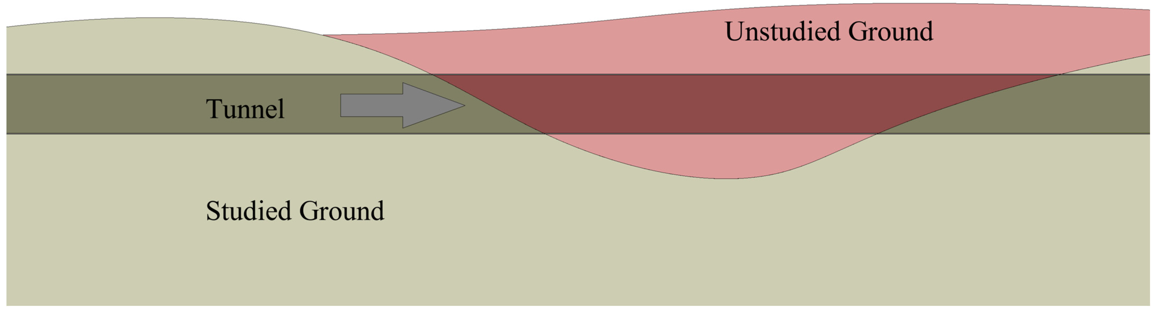
In this paper, the implementation of transfer learning is investigated in the context of tunnel engineering for two objectives. The first is the simulation of a sudden change in ground conditions during a tunneling project, as illustrated conceptually in Figure 1. For this scenario, it is assumed that the initial ground has been sufficiently monitored and studied, and only a limited amount of data has been collected for the newly encountered (unstudied) ground. Accordingly, it is investigated whether transfer learning can overcome the shortage of data for the unstudied ground.

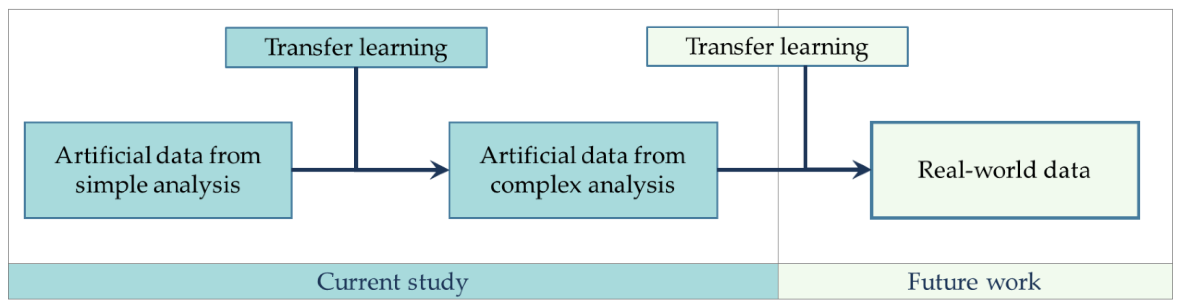
The second study aims to investigate whether learning can be transferred from simple to more complex data. For this purpose, two datasets are created: (1) a large dataset from a simplified hydrostatic stress field analysis, and (2) a small dataset from a more complex and realistic non-hydrostatic loading. Successful implementation of transfer learning on these tasks can be interpreted as an indication that simpler artificial data can be used to augment the more complex real-world data, as illustrated in Figure 2. Potentially, data generated via numerical simulations could be used to pre-train an initial ML-model and transferred to learn the data collected in-situ. This could help overcome the technical limitation of the size of data needed for ML, as a vast amount of artificial data can be generated from FE models with minimal costs. As stated in Figure 2, whether the results of the current study apply to the transfer of knowledge to real-world settings requires further work.

Hereinafter, the paper is organized as the following:

• First, a brief review of the relevant background information for tunnel support analysis and ML is provided.
• Second, the methodology and implementation of transfer learning for the simulation of the first scenario of a change in ground conditions is presented.
• Third, following the same methodology as the first scenario, the implementation of transfer learning from simple to complex tunnel support analysis is presented.
• Fourth, the results of both investigations are presented and discussed.
• Finally, the conclusions and limitations of the current work are summarized.

2. Background Information

2.1. Tunnel Support Analysis

A number of different approaches are regularly used in conjunction for the stability analysis of tunnels, including analytical, empirical, and numerical methods. Analytical methods are limited to a set of simplifying assumptions that allow for a precise mathematical solution, and empirical methods are limited to the settings of their case studies [8]. In contrast, numerical methods based on the finite-element (FE) method are capable of simulating irregular geometries and complex material models. However, the assessment of ground strength parameters often relies on empirical methods and subjective judgment.

An analytical approach which is widely studied and used for tunnel support analysis is the convergence-confinement (CC) method. The CC method is based on three main independent components:

• The ground convergence curve
• The support curve (confinement)
• Initial displacement prior to the support

Numerous solutions for ground (or tunnel) convergence curves and for support response have been published ([9,10,11]). These solutions assume mainly elastoplastic Mohr–Coulomb behavior and vary primarily by their post-peak behavior, as well as modifications for other unique conditions. The CC method is used primarily for weak rock tunneling, but can be applied to other interaction problems, such as room and pillar mining [12].

Once both the tunnel convergence and support curves are plotted, their point of intersection shows the final displacement of the supported tunnel. Inevitably, some displacement occurs prior to support installation. This initial displacement occurs mainly on the longitudinal distance between the tunnel face and point of support installation. In the CC plot, this initial displacement dictates the origin of the support curve. For the current work, it has been assumed that the support is installed at the tunnel face. Note that some initial displacement occurs even at the tunnel face [13]. Figure 3 shows an example of a CC plot, where the point of curve intersection defines the system-equilibrium displacement by its reflection on the horizontal axis. This figure has been generated via the commercial program RocSupport which relies on the CC approach [14]. The parameters that dictate the slope of the ground response curve are the ground’s Young’s-modulus and uniaxial strength. The former determines the initial slope of the curve, and the latter dictates the point of transition to a non-linear curve. Post-peak behavior is computed according to the development of a plastic radius around the tunnel contour.

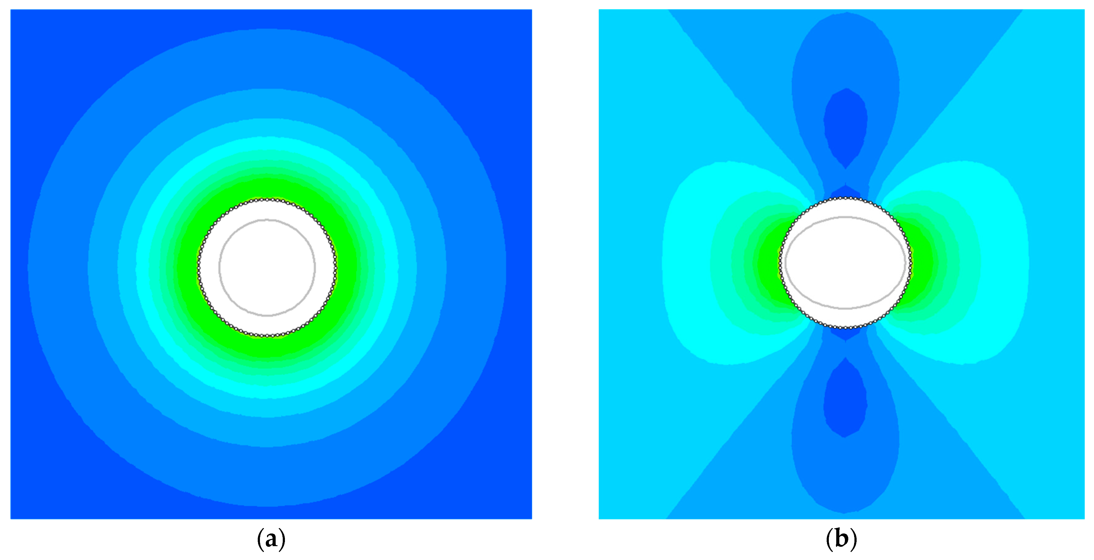
In order to obtain closed-form solutions of GRCs, the simplifying assumption of axisymmetric conditions is made. The axisymmetric assumption requires that the shape of the tunnel is circular and that the in-situ stress field is hydrostatic (i.e., the vertical stresses are equal to the horizontal stresses). Hence, the displacement of the tunnel is uniform. While many tunnels are circular, the assumption of a hydrostatic stress field is an over-simplification of reality, as it neglects significant phenomena such as ground arching and liner bending [15]. Figure 4 shows an example of the stress field and deformation for hydrostatic and non-hydrostatic loading conditions, generated via the RS2 program.

Compared to FE modeling, the CC approach has the advantage of explicitly providing a factor of safety, which is useful for design purposes. However, there are available methods for enhancing FE analysis to include stability assessment, such as the FE limit analysis [16,17].

2.2. Machine-Learning

The immense advancement of computing power and digital data ML algorithms have emerged as powerful computational tools for applications that require the analysis of large sets of data. ML has been recognized as a potential tool for revolutionizing the field of geological engineering by collecting extensive field data via digital instrumentation and correlating it to various measurable ground responses [18]. The main obstacles of actualizing many potential applications of ML for such research projects is related to the acquisition of data. The cost of monitoring device installation is great and, in many projects, limited reliable data are generated. Moreover, the generated data often require extensive efforts to prepare the data for ML.

Another potential use of ML involves coupling it with artificial data generated by numerical modeling. This type of coupling is often referred to as surrogate modeling. An excellent review of the concept of surrogate models is presented by [19]. Surrogate models allow for fast and rigorous data analysis and help provide insights that may otherwise remain unrecognized.

There are many available models for ML, each with pros and cons. Artificial neural networks (ANNs) are a collection of nodes that receive input numbers and pass on some other number to the subsequent nodes on the network. Using a training process referred to as back-propagation, the values in each node are adjusted to minimize the error between the inputs and outputs. ANNs allow for the identification of subtle patterns in large and complex datasets. However, ANNs generally perform poorly on small datasets and simpler ML methods, such as random forest (RF), are more suitable for training small datasets [20]. RF is an ensemble method where multiple decision trees are assessed, and the correlation between input and output data is established according to a majority vote. RFs are robust methods and have been found to perform well for small datasets [21]. Another advantage of RFs compared to ANNs is that they are less sensitive to hyper-parameters and therefore require less fine-tuning.

Transfer learning is a technique in ML that allows for extracting knowledge obtained from a large dataset and transferring it to different but related task with a smaller dataset. Ref. [22] provide an intuitive illustration of this concept: learning how to play the piano would demand less effort if the person already knows to play the guitar. The major benefit of this technique is overcoming the limitation of dataset size. There are other benefits to transfer learning, including reducing overfitting and decreasing the time and computational resources required to train a model. Transfer learning is regularly achieved by freezing the initial ANN. Subsequently, the training process for the smaller dataset is executed either by starting with the initialized weights and biases from the original model or by adding an additional layer and fitting it to the new data. For the current paper, the second method is used.

Different researchers have demonstrated the use of coupling ML tools with geotechnical analysis. For example, ref. [23] analyzed numerical models of tunnels with ANNs in order to investigate the stability of the tunnel face. Ref. [19] used ML models to investigate different problems with rock mechanics. However, it is important to remember the limitations of such applications, as ML is used to enhance and accelerate numerical modeling, rather than discovering new knowledge. Ref. [18] discusses the opportunities of utilizing in-situ data from tunnels and mines for overcoming knowledge gaps in rock mechanics.

Transfer learning has been applied to several fields [22]. A number of researchers have recently published works where transfer learning is used for tunnel engineering applications. Zhou et al. [24] proposed applying transfer learning for predicting tunneling-induced surface settlements. Ref. [25] used a transfer learning technique to extract knowledge from historical databases for predicting cutterhead torque in TBMs. Ref. [26] studied the application of transfer learning for an image recognition task to classify cracks in tunnel liners.

3. Transfer Learning for Change in Ground Conditions

In order to examine the problem described in the introduction and illustrated in Figure 1, the following scenario was assumed. A circular tunnel with a 14 m diameter is to be driven through weak ground. Tunnel liner elements are 450 mm thick and made of concrete with 45 MPa uniaxial strength. While the majority of the ground is anticipated to be from a single geological formation, it is likely that unknown formations will be encountered. In this case, it is important to respond promptly and implement the appropriate measure (e.g., reinforcement of the ground or support, stopping excavation, etc.). The in-situ stresses are mainly tunnel depth and soil weight and are assumed to vary as well.

Table 1. Dataset #1 (DS1), #2 (DS2), and #3 (DS3) input parameter range and tunnel displacements computed via the CC method.

		Friction Angle	Cohesion	In-Situ Stress	Uniaxial Strength	Young’s Modulus	Tunnel Displacement
Units:		Degrees	MPa	MPa	Mpa	Mpa	mm
DS1 (n = 200)	Min.	22.5	0.35	8	1.05	524	34
	Mean	30	0.5	10	1.73	1053	122
	Max.	37.5	0.65	12	2.64	1582	504
DS2 (n = 25)	Min.	20	0.3	8	0.86	383	124
	Mean	25	0.35	9	1.08	510	308
	Max.	30	0.4	10	1.37	660	627
DS3 (n = 25)	Min.	40	0.1	6	0.43	339	43
	Mean	45	0.15	7	0.72	574	97
	Max.	50	0.2	8	1.10	809	190

lists the statistics (minimum, mean, and maximum) of the soil input parameters used for three datasets, denoted DS1, DS2, and DS3. These datasets represent three varying soil formations according to the following rationale:

• DS1—represents a soil where a significant amount of data has been collected and consists of 200 rows of input parameters.
• DS2—represents a new soil formation with only 25 rows of input parameters. This soil is slightly weaker than DS1, with a significant overlap of parameter range compared to DS1.
• DS3—represents a new soil with a small dataset, similar to DS2. In contrast to DS2, DS3 has very little overlap with DS1 parameters.

With respect to the soil parameters listed in Table 1, the friction angle, cohesion, and in-situ stress are assumed, and the uniaxial strength and Young’s modulus are computed according to the relationships given in Equations (1) and (2):

$$\sigma =\frac{2\ast c\ast cos\mathrm{\varnothing }}{1-sin\mathrm{\varnothing }}$$

(1)

$$E=MR\ast \sigma$$

(2)

where $\sigma$ is the soil uniaxial strength, c is the cohesion, $\varnothing$ is the friction angle, E is the Young’s modulus, and MR is an empirical modulus ratio. Note that a modulus ratio is usually used for rock mechanics applications [27], and laboratory and field tests are usually used for Young’s modulus estimation for soil. This simple linear relationship is used here for the sake of simplicity. However, in order to add another degree of noise, MR is randomly varied using different ranges for each dataset.

The tunnel displacements are computed using the CC method. The commercial program RocSupport was developed to allow for rapid calculation of tunnel displacements and support pressures according to different conditions and methods [28]. A Python script was written to automate the computation process of this program and calculate the tunnel displacements for each set of input parameters. The solution derived by [29] is used for the ground response curves. As part of the CC solving process, the plastic radius around the tunnel is computed. The mathematical derivation of the plastic radius is given by [13]. Ultimately, each dataset consists of an input matrix of four parameters in each row: in-situ stress, uniaxial strength, Young’s modulus, and the resultant plastic radius. The output parameter is a column vector that consists of the corresponding tunnel displacements.

All ML programming is carried out in Python via the Keras open-source library [7]. In order to investigate the effect of transfer learning, an initial ANN referred to as NN1 is trained on DS1, to be later modified to predict the smaller datasets DS2 and DS3. This training process involves fitting the input parameter matrix to the tunnel displacement column vector. Subsequently, NN2 and NN3 are created in order to transfer the learning from DS1 to DS2 and DS3, respectively.

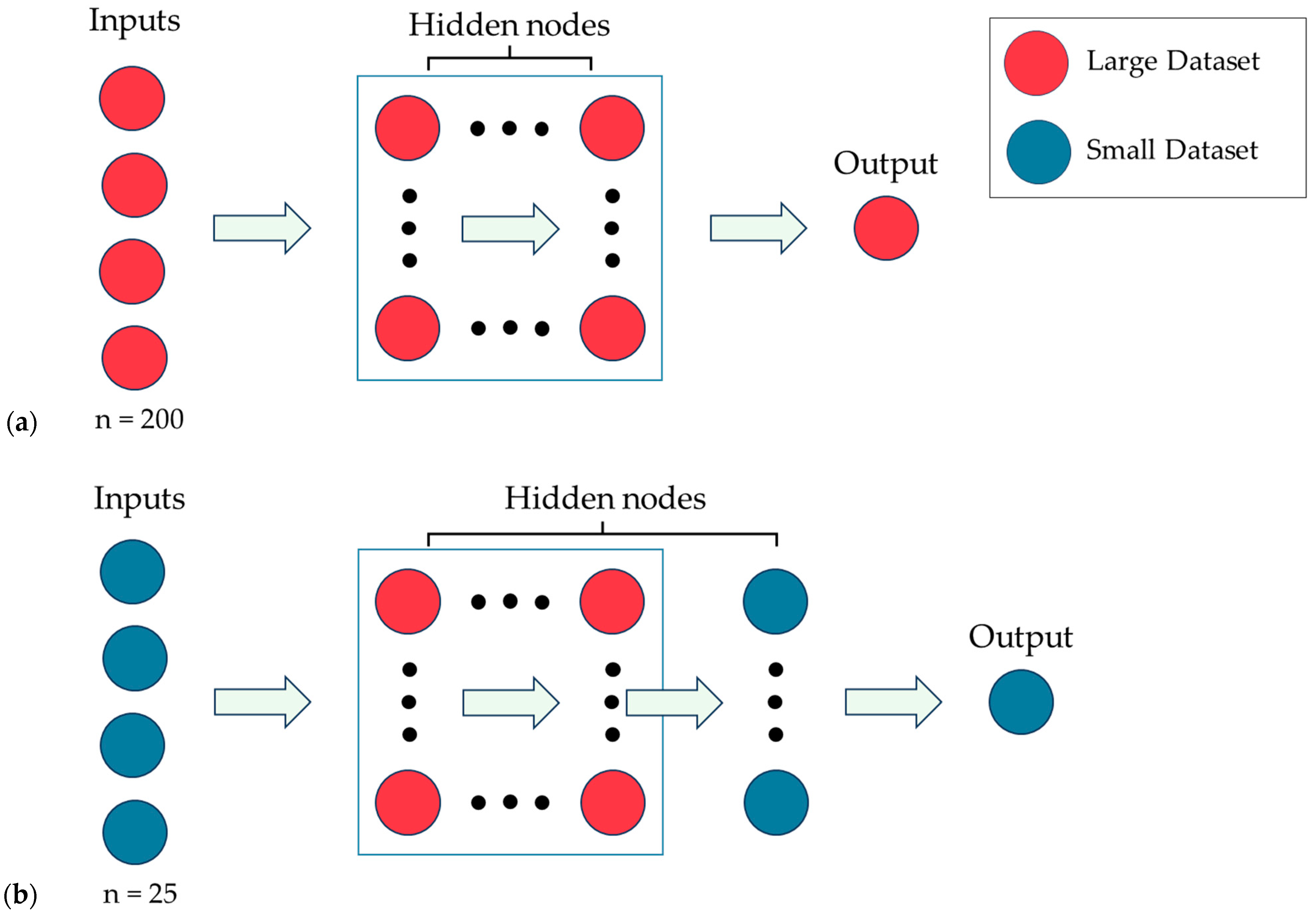
The technical procedure for transfer learning undertaken in this paper is illustrated in Figure 5. Figure 5a shows the four nodal inputs, which are the input parameters from each row of DS1. These inputs are passed to the hidden nodes. The arrows in the figure represent dense connections, i.e., the output of each neuron in the subsequent layer is based on the input from each neuron in the preceding layer. In ML practice, the optimal number of hidden neurons cannot be pre-determined. Therefore, it is customary to compare different network architectures and select the one that is most accurate. After the hidden nodes and other hyper-parameters are fine-tuned and the accuracy of ANN is found to be sufficient, NN1 is stored in its final numerical configuration.

Figure 5b shows the second ANN, NN2, for the transfer learning task. For the current analysis, the blue nodes (sometimes referred to as neurons) represent the network components of the smaller dataset, i.e., DS2 or DS3. A new ANN for transfer learning is created and referred to as NNT. For this purpose, the inputs and outputs for the smaller dataset are connected through NN1 and an additional hidden layer that precedes the output node. NN1 is frozen in its original state, whereas the additional layer is subject to fine-tuning.

In order to investigate the effect of noisy data, a Gaussian generator was used. After computing results with no noise, the computation was repeated with noise standard deviations (NSD) of 5% and 10% that were added to all inputs and outputs in each dataset.

A number of metrics are available for evaluating ML performance, including the coefficient of determination, mean absolute error, and root-mean-square error (RMSE), among others. For example, RMSE = 50 mm would indicate that, on average, the model’s predictions deviate by 50 mm from the actual results. In order to provide an intuition for ML model performance and RMSE, a model that always predicts the mean displacement is generated and the corresponding RSME is found to equal approximately 70 mm.

Fine-tuning ANN architecture and hyper-parameters is a subject of ongoing research [30]. Hyper-parameters are the parameters that are not part of the studied problem but impact the learning process. There are different methods for selecting the optimal combination of hyper-parameters, the simplest being manual tweaking. However, manual adjustments based on trial and error are time consuming and are also less likely to lead to optimal results. A grid search is a rigorous method where different combinations of hyper-parameters are examined. Advanced methods include the application of optimization algorithms, such as the genetic algorithm. The effort invested in the fine-tuning process is dependent on the level of accuracy required for the specific application. For the current work, the objective of the analysis is largely for the sake of evaluating transfer learning success rather than obtaining very high accuracy. The method used was a random search where, through an iterative process, the ANN was repeatedly computed with randomly varied hyper-parameters. The number of layers, number of nodes in each layer, learning rate, batch size, activation function, and regularization strength were varied in each iteration, and the corresponding RMSE was found. In this study, a single hidden layer of nodes performed better than two and three layers. The hyper-parameters selected for NN1 with no noise were 16 nodes, a learning rate of 0.001, a regularization strength of 1%, a batch size of 32, and the softplus activation function. These hyper-parameters were slightly modified for the noisy datasets. For NT, where an additional layer was added, minimal fine-tuning was carried out, as only the number of nodes and batch size were altered.

4. Transfer Learning for Simple to Complex Analysis

The hydrostatic assumption (i.e., horizontal to vertical stress ratio K = 1) made for the CC method is a significant simplification with respect to reality, as discussed in Section 2.1. In this section, a large dataset, DS1, made of 200 rows, is created according to the hydrostatic loading assumption, representative of simplistic analysis. Similar to the previous section, two small datasets of 25 rows are created where more realistic non-hydrostatic loading conditions are applied. For both small datasets, DS2 and DS3, the K ratio varies from 0.3 to 0.7. With respect to the ground strength parameters, DS2 is identical to the large dataset DS1, and DS3 consists of a different range of strength parameters.

Table 2. Range of input parameters and tunnel displacement for the datasets.

		Friction Angle	Cohesion	Young’s Modulus	Tunnel Displacement
Units:		Degrees	MPa	MPa	mm
DS1 (n = 200) DS2 (n = 25)	Min.	20	0.35	500	35
	Mean	30	0.5	1000	64
	Max.	40	0.65	1500	139
DS3 (n = 25)	Min.	20	0.15	1000	37
	Mean	30	0.3	1500	71
	Max.	40	0.45	2000	140

shows the variation of the input parameters and displacements for the datasets.

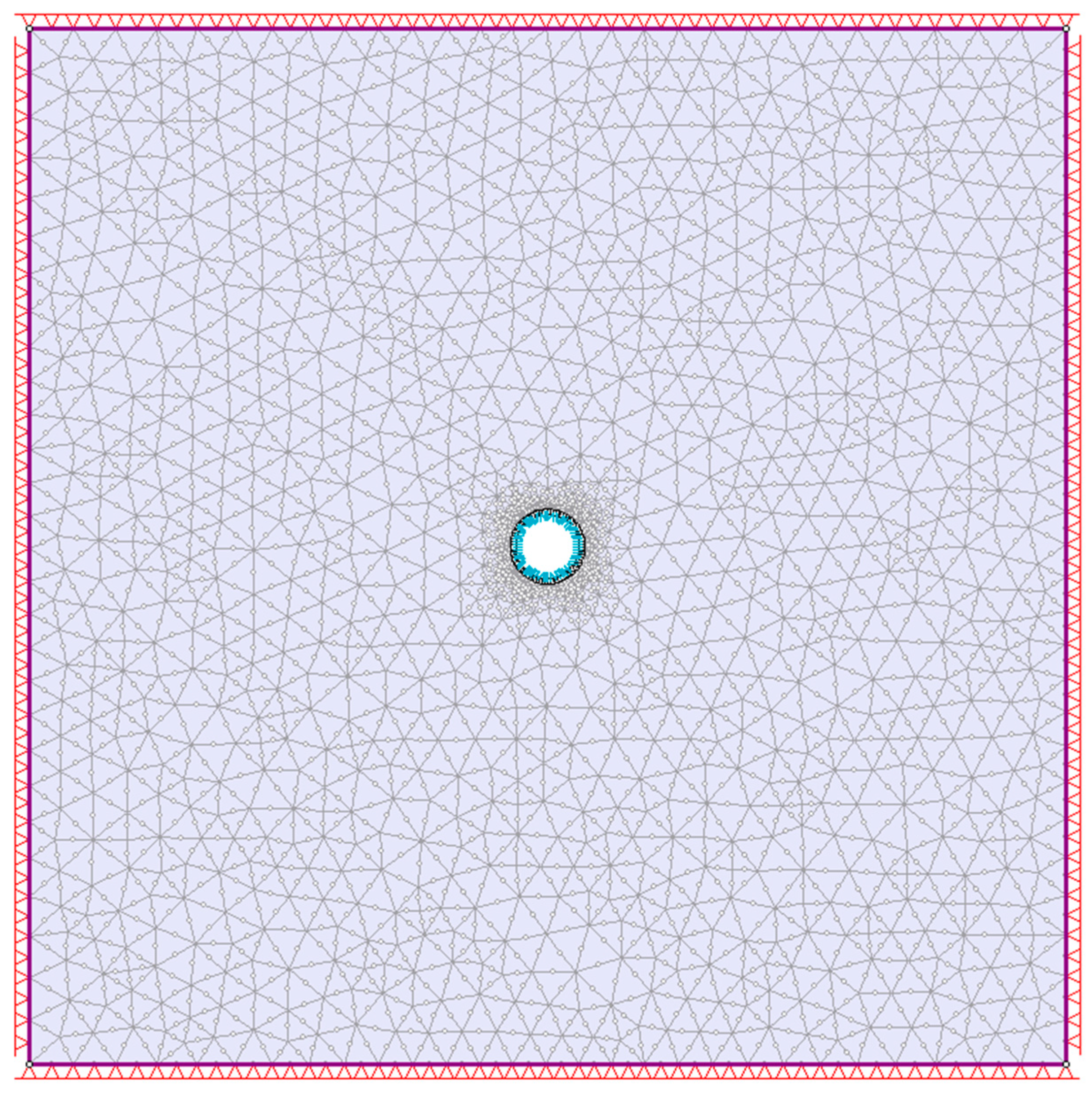
Displacement results computed with the CC method and from FE models with hydrostatic loading may differ for various reasons. Hence, for the current analysis, all the results were computed with the commercial FE code RS2 [28]. Figure 6 shows the model geometry and mesh. For all datasets, the tunnel diameter is 14 m, the liner thickness is 450 mm, and the vertical stress is 10 MPa. In order to account for the initial displacement prior to support installation, the FE model loading is staged, where 30% (i.e., 3 MPa) of the load is applied upon the unsupported tunnel in the first stage, and 70% (i.e., 7 MPa) is activated on the supported tunnel in the second stage.

Ultimately, each dataset consists of an input matrix of four parameters in each row: in-situ stress, uniaxial strength, Young’s modulus, and the K ratio. Note that the plastic radius is not included as a feature for this analysis because this parameter is only valid for hydrostatic loading. For the non-hydrostatic loading, the plastic zone around the tunnel is not circular. In addition, for non-hydrostatic loading, the displacements vary along the tunnel contour. The maximum displacements occur at the tunnel crown and are passed to the output column vector.

The methodology for ML analysis undertaken in the previous section is generally repeated for the current investigation. In brief, DS1 is trained with NN1, and transfer learning is carried out with NNT. NNT is created by freezing NN1 and adding an additional layer. The process for adding noise is identical to the previous section. In order to gain an intuition of the RMSE, a model that predicts the mean displacement for every instance was generated, and an RMSE of 55 mm was yielded.

Based on a randomized search, hyper-parameters were selected for NN1. In this process, it was found that two hidden layers perform better than a single hidden layer. Accordingly, the following hyper-parameters were selected for the ANN with no noise: 32 nodes for the first and second hidden layer, a learning rate of 0.0001, a batch size of 16, and the ReLU and Tanh activation functions. The hyper-parameters selected for NNT are 16 nodes in the additional layer and a batch size of four. These hyper-parameters were slightly modified for the noisy datasets.

5. Results

In order to determine whether transfer learning is effective, two conditions must be satisfied:

• The accuracy of N1 predictions on the small datasets DS2 and DS3
• The accuracy of a new ML model for predicting DS2 and DS3

With respect to the first condition, it was found that even after fine-tuning of the hyper-parameters, ANNs failed to provide valid predictions for the smaller datasets in both investigated scenarios. In addition, RF models, considered ideal for small datasets, also performed poorly on this task.

In order to examine whether the second condition is satisfied, the RMSE was computed for DS2 and DS3 with NN1 and NNT. Since small datasets are prone to high variance, two additional datasets of 25 rows were generated, and the mean RMSE was taken according to an average of both results.

The results of the analysis for the first scenario (i.e., change in ground conditions) are listed in

Table 3. Summary of performance of ANNs under different noise standard deviations (NSD).

		RMSE [mm]
ML-Model	Dataset	NSD = 0%	NSD = 5%	NSD = 10%
NN1	DS1	14	16	19
NN1	DS2	102	95	106
NNT	DS2	41	56	65
NN1	DS3	37	40	39
NNT	DS3	21	22	24

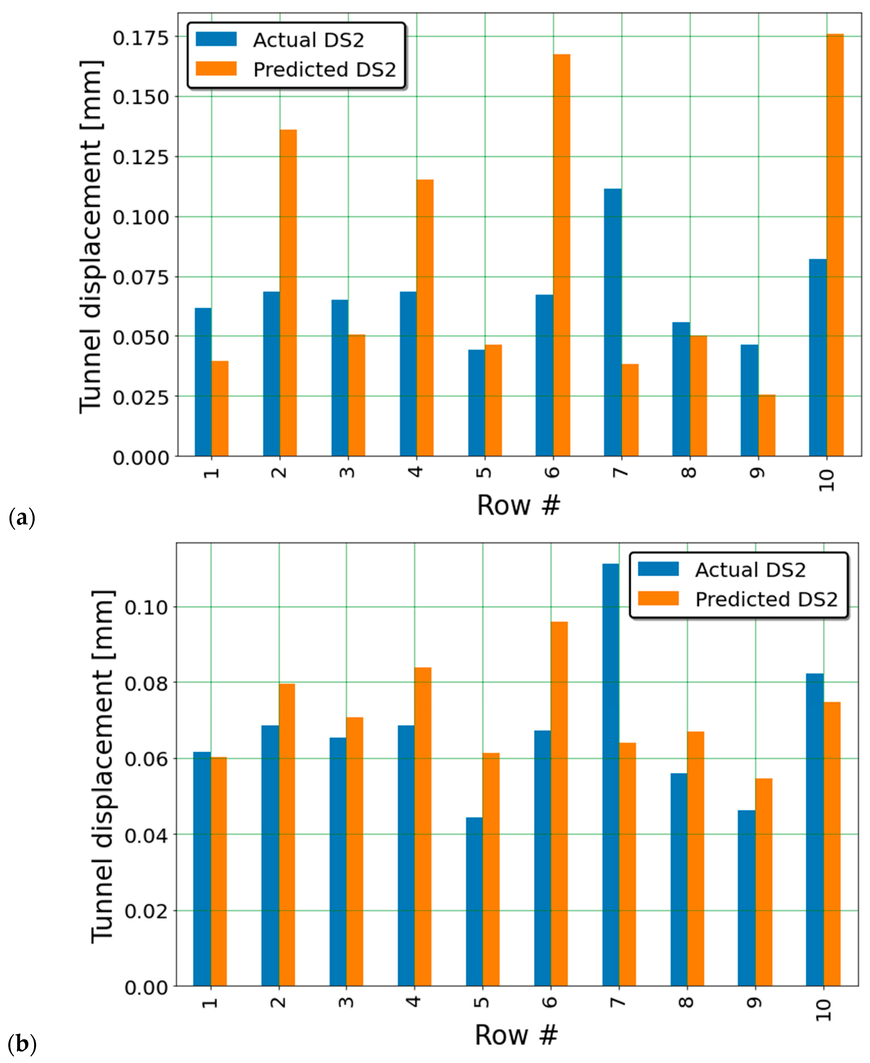
. Results demonstrate that implementation of transfer learning leads to a significant improvement in accuracy for both datasets and under every NSD. Figure 7a,b show the predictions and actual displacements for a sample of 10 rows from DS3 with NSD = 5% computed with NN1 (without transfer learning) and NT (with transfer learning), respectively.

As mentioned, it is important to bear in mind that ANNs are susceptible to errors and inconsistencies, as they are highly influenced by hyper-parameters [7]. Moreover, other sources of randomness (e.g., random weight initialization) may alter the results of ANNs, even without changing hyper-parameters. Such inconsistencies can be observed in Table 3 itself, as the RMSE is expected to increase with increasing noise, yet this is not always the case.

For the second scenario (i.e., learning from hydrostatic to non-hydrostatic conditions) results are listed in

Table 4. Summary of performance of ANNs under different noise standard deviations (NSD).

		RMSE [mm]
ML-Model	Dataset	NSD = 0%	NSD = 5%	NSD = 10%
NN1	DS1	2	3	7
NN1	DS2	40	51	59
NNT	DS2	26	29	33
NN1	DS3	41	37	54
NNT	DS3	14	18	20

. Results show that transfer learning improves ML performance for both datasets and for every NSD. Compared to the analysis conducted for the first scenario, the relative RMSE of the small datasets is greater (see Table 3). A possible explanation for the greater error in the current analysis is that the tunnel behavior is substantially different under hydrostatic conditions. In contrast, in the previous analysis only the ground properties were changed. In addition, the omission of the plastic radius feature that does not apply to the current analysis may also have a negative impact on ML performance.

Comparing the RMSE of NN1 and NNT for DS2 and DS3 shows that transfer learning brings improved correlation in of the instances. Figure 8 shows an example of predictions vs. actual displacements with and without transfer learning for DS3 with NSD = 10%. The benefit of transfer learning is apparent in the figure. This finding indicates that there is potential for artificial data to enhance real-world data. However, these results should be interpreted with caution, as real-world data is likely noisier and more complex compared to the current data. Indeed, more work is required where artificial data and real-world data are analyzed.

Comparing NNT performance on DS2 and DS3, the latter was found to be more accurate. This is somewhat counter-intuitive, as different ground parameters are assigned to DS3. This reflects upon the black-box nature of ML, as the internal learning process of ANNs is not interpretable to the user.

6. Summary and Conclusions

In order to investigate the implementation of transfer learning for tunnel support analysis, two scenarios were investigated: (1) transferring knowledge between different ground formations, and (2) transferring knowledge from simplified hydrostatic loading to a more complex and realistic non-hydrostatic stress field. The objective of the second scenario is to examine the potential of enhancing real-world data with data generated via numerical simulations (see illustration in Figure 2).

The technical process for implementing transfer learning involved training an ANN on an initial large dataset with a size of 200 rows, and then adding an additional layer and training it on small datasets of 25 rows. Subsequently, the ANNs were tested on unseen data, and the RMSE was computed. In order to conclude that transfer learning is effective, two conditions were checked: (1) the RMSE from transfer learning is lower than the RMSE from an RF model trained solely on the small datasets, and (2) the RMSE from transfer learning is lower compared to predictions made with the original ANN trained on the large dataset. In order to better mimic reality, numerical noise was added to the datasets. The analysis was repeated for each of the scenarios for varying degrees of noise.

As expected, increasing the degree of noise caused the RMSE to increase. Nevertheless, the improvement due to transfer learning was consistent throughout all investigations of both scenarios. A comparison of the results of the two scenarios shows that lower accuracy is achieved for the second task. The apparent explanation for this is that transferring knowledge between analyses with different tunnel behavior is less effective than transferring knowledge between identical behavior with different strength parameters.

To summarize, the findings in this paper highlight the potential of transfer learning as a powerful technique for overcoming dataset size limitations. The results demonstrate the effectiveness of this technique and suggest that it would be possible to synthesize artificial data with real-world data. The prospect of transfer learning should motivate researchers, engineers, and other stakeholders to invest in in-situ data collection for the sake of ML analysis. The general methodology presented in this paper could be applied and further modified for the analysis of other applications. For this reason, we have made our data and code available online [31]. It is anticipated that, following further development and refinement, transfer learning will become a fundamental part of ML-related works in geotechnical applications.

7. Limitations

It is important to acknowledge the limitations of the current study. Firstly, the fields of data science and artificial intelligence are rapidly advancing, with transfer learning being in its nascent state. Hence, technical details and results (e.g., size of datasets, ANN architecture, and hyper-parameters) should be interpreted with caution. Each case study requires special analysis and judgment regarding optimal ML analysis procedures while staying up to date with the latest developments in this field.

Secondly, the current analyses rely on artificial data. While the addition of noise generally assists in bridging the gap from model to reality, there is still a lack of research that provides guidelines for selecting signal-to-noise ratios that are representative of geological materials.

Finally, integrating ML tools with geotechnical analysis is still in its infancy. As a result, there are no available guidelines for the implementation of ML in compliance with standard design procedures. The execution and evaluation of ML algorithms implicitly impacts the assessment of safety factors. Further research is necessary for developing procedures for the proper integration of ML with established design procedures.