
Multi-Task Learning Approach Using Dynamic Hyperparameter for Multi-Exposure Fusion

Abstract
:1. Introduction
- To train MEF networks that require learning, we present a method for setting up a customized dataset;
- To generate multiple tasks based on source features, we perform a procedure that filters unnecessary regions from the source images using multi-exposure image characteristics;
- To reflect the information between multiple tasks, we set dynamic hyperparameters on the loss functions. This helps the network reproduce better-contrast images;
- To produce a high-quality image with a simple network design, we prove that it is possible to utilize multiple tasks and dynamic hyperparameters for the loss function.
2. Related Works
2.1. Multi-Exposure Image Fusion
2.2. Deep-Learning-Based Multi-Exposure Image Fusion
3. Proposed Methods
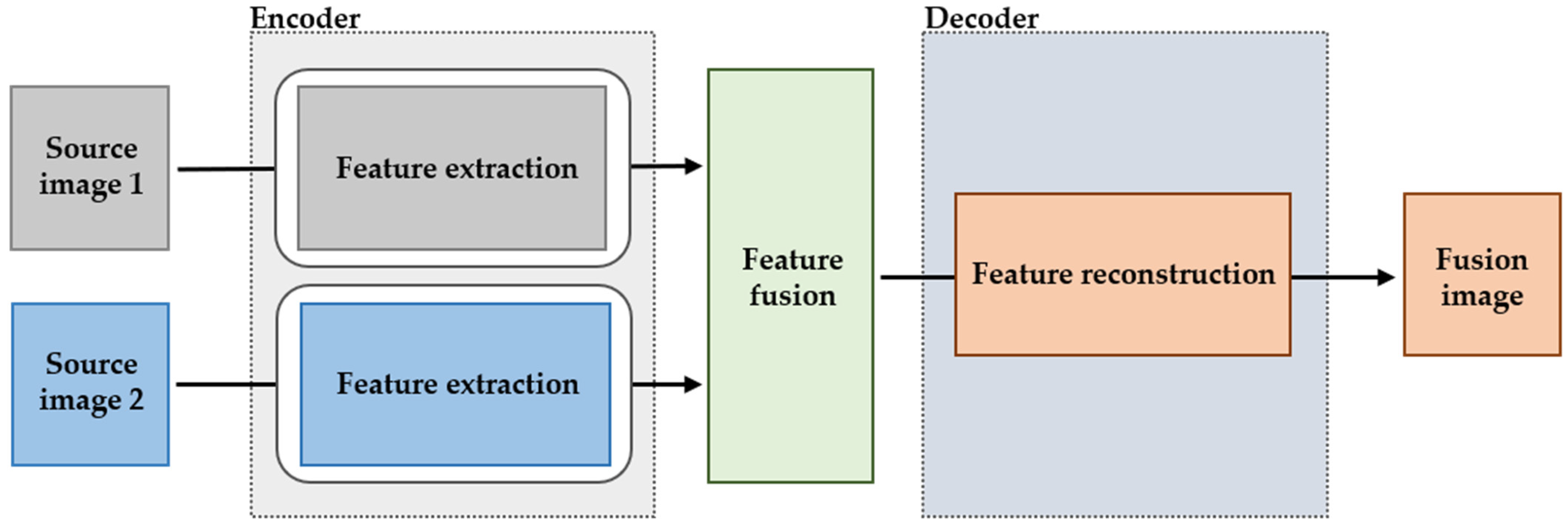
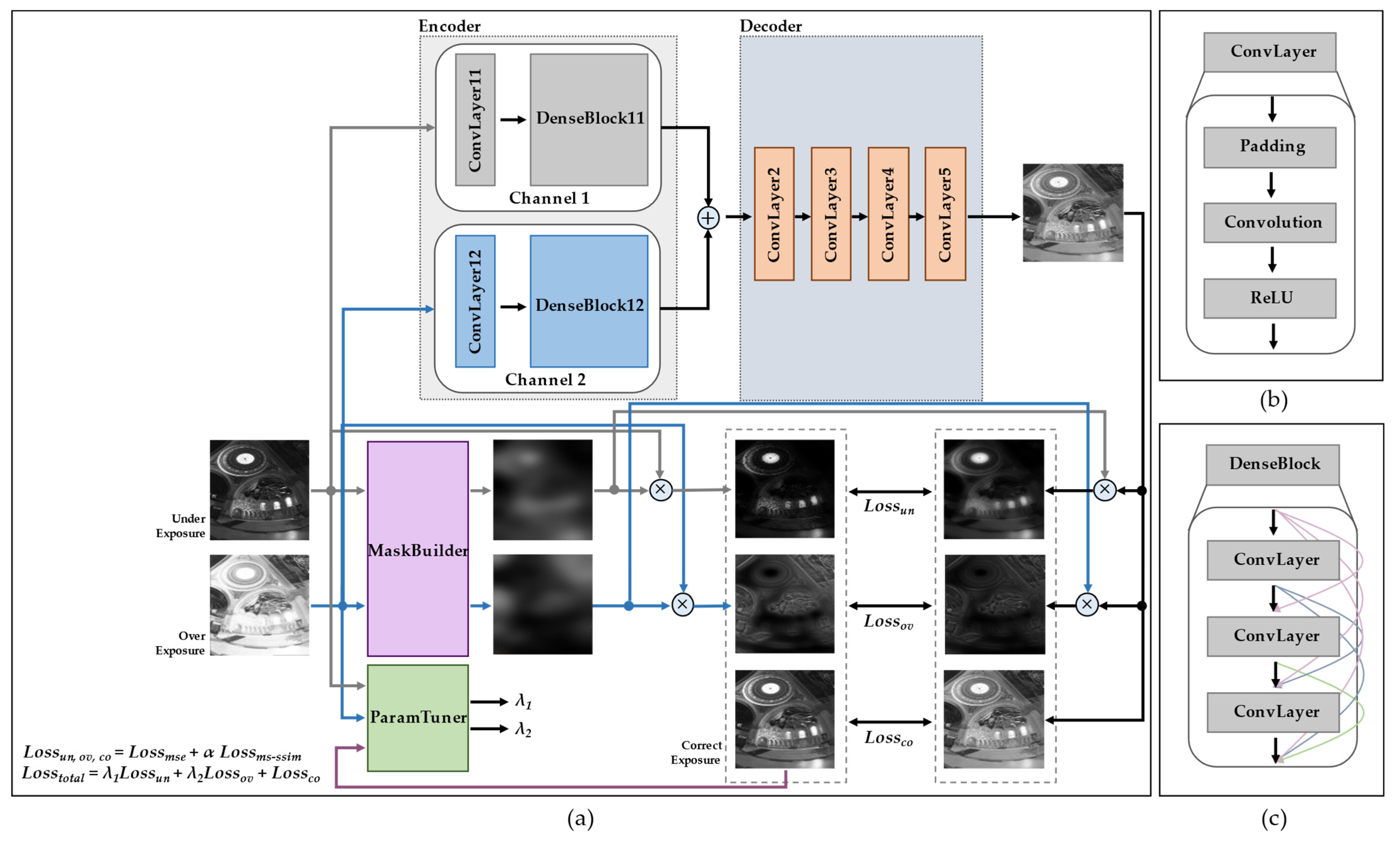
3.1. Framework Overview
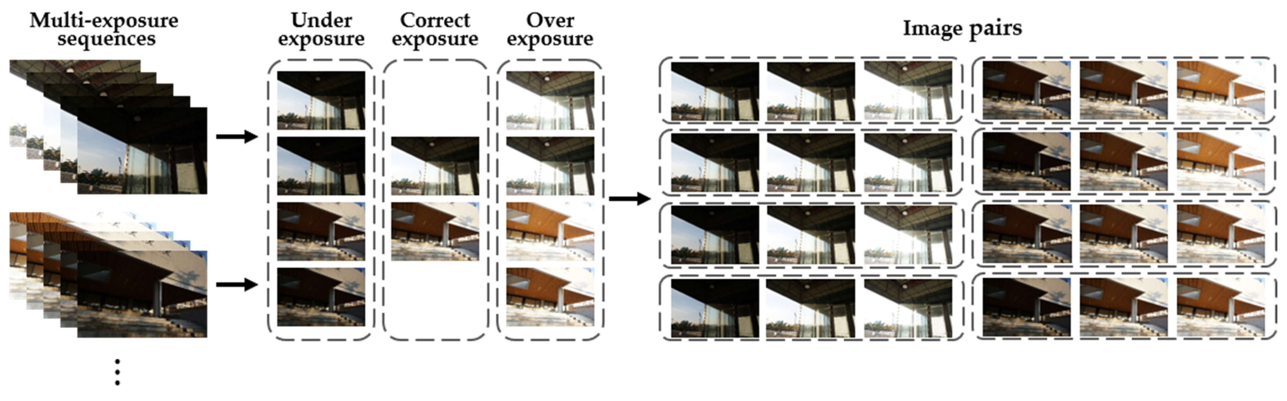
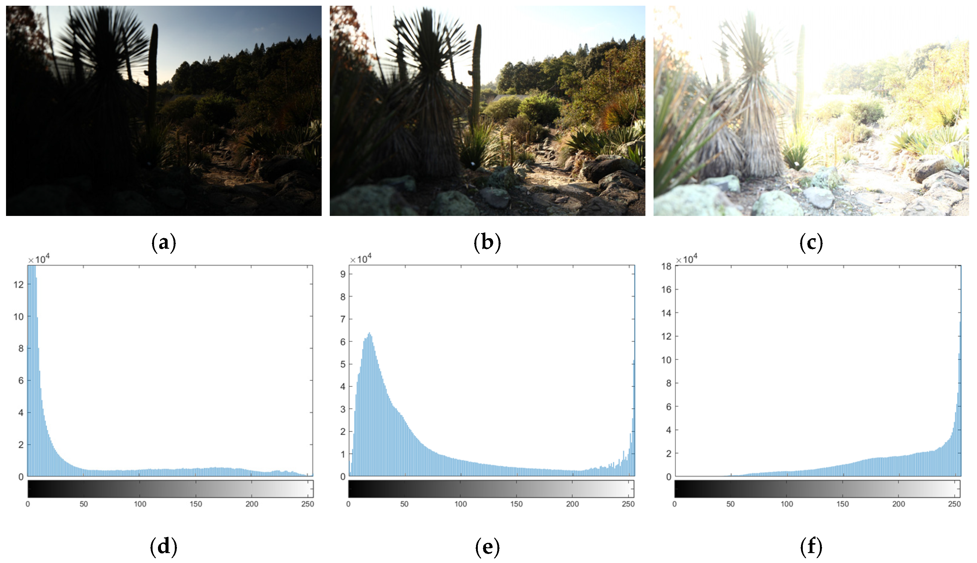
3.2. Dataset Acquisition
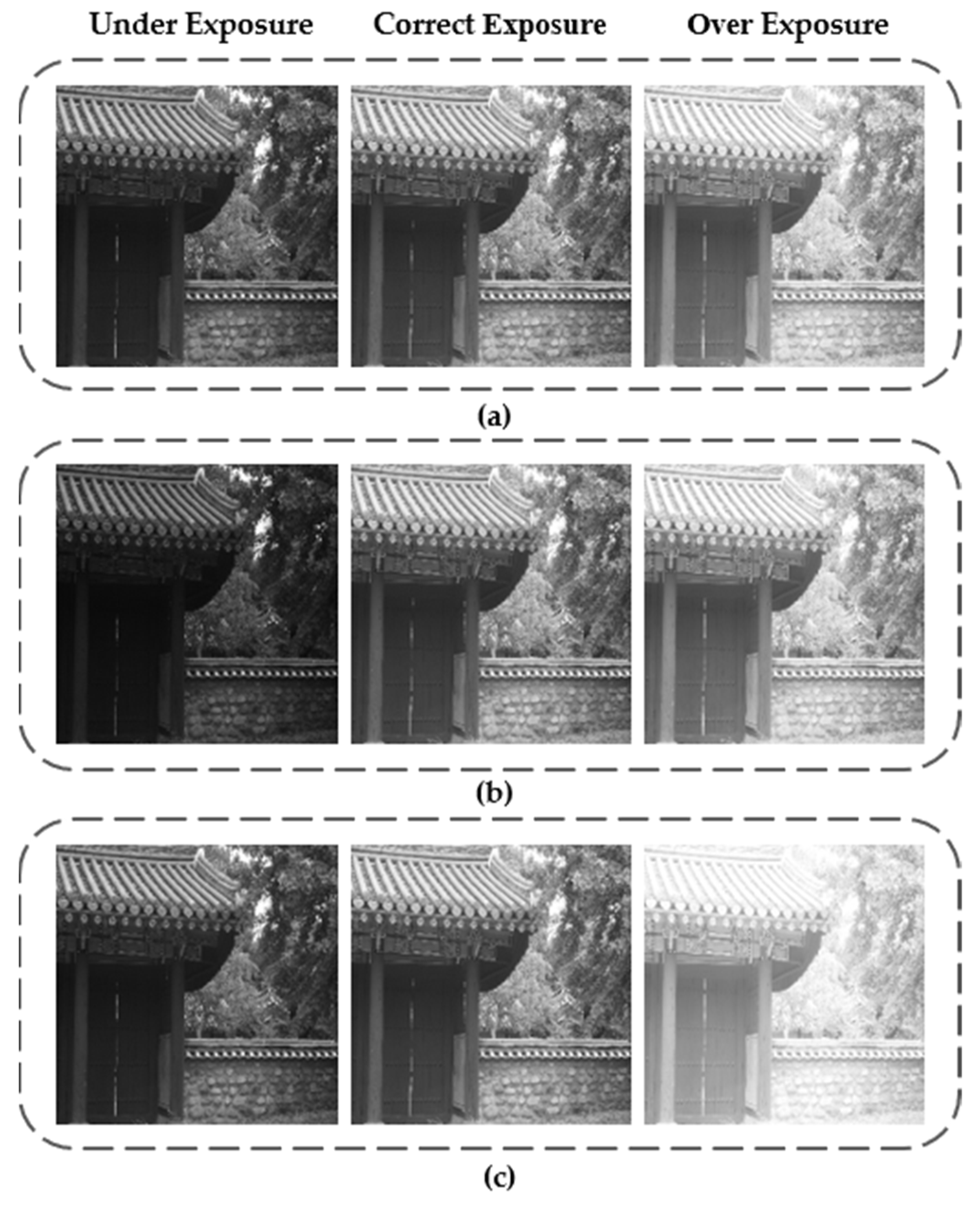
3.3. MaskBuilder
3.4. Loss Function
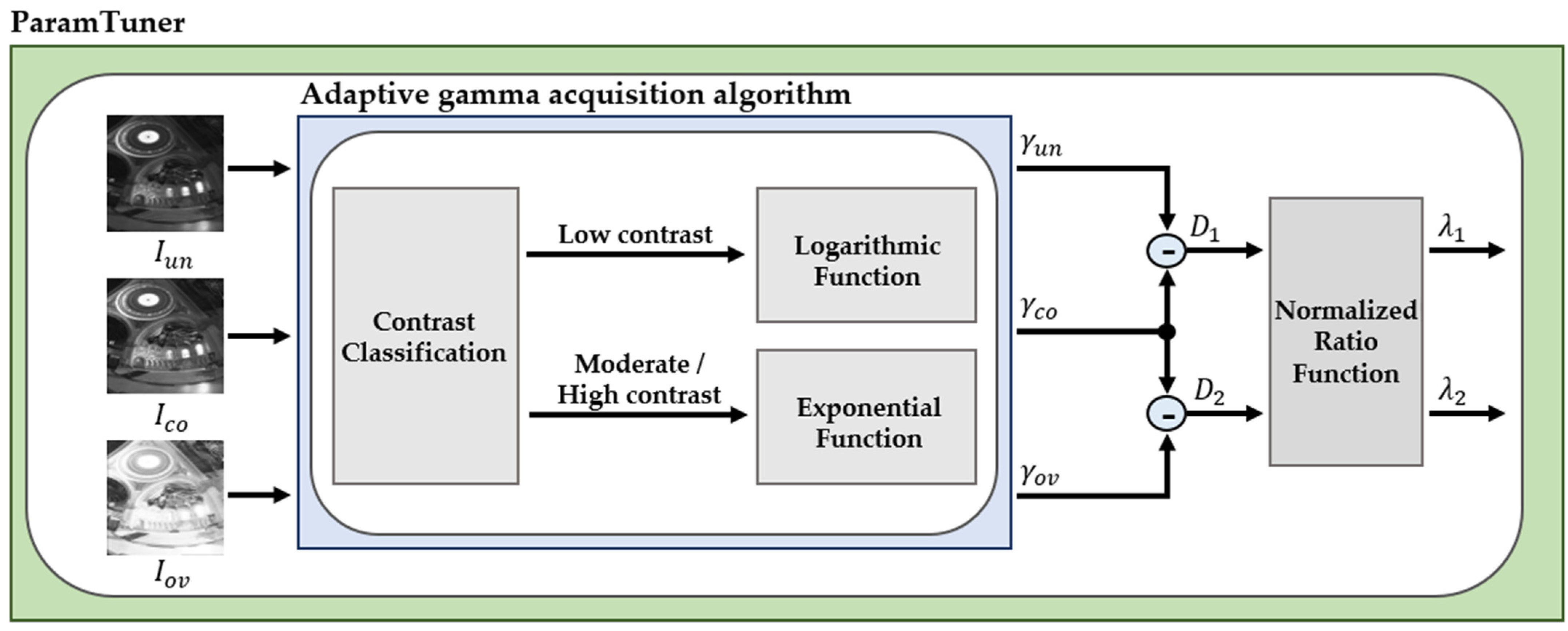
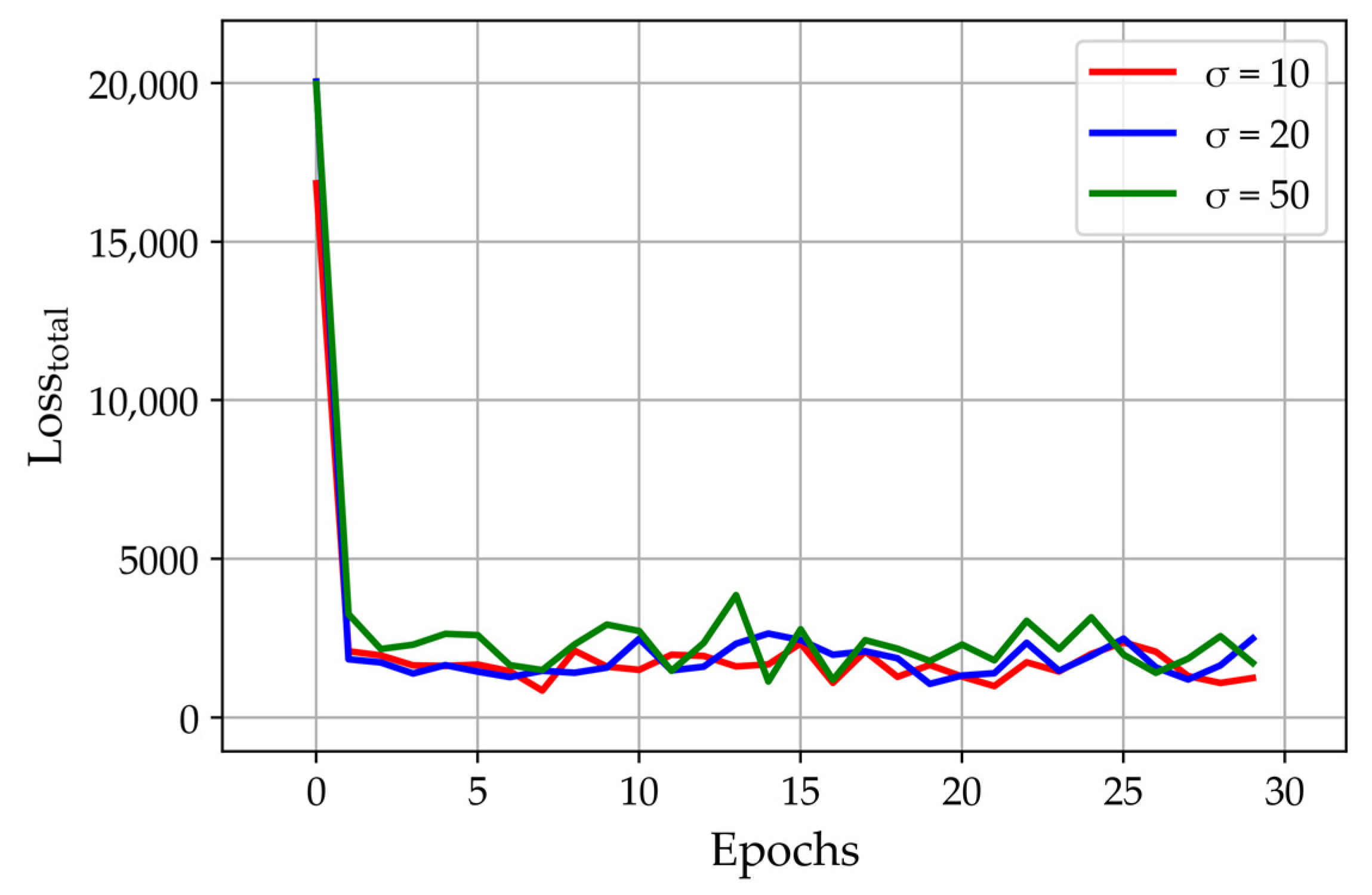
3.5. ParamTuner
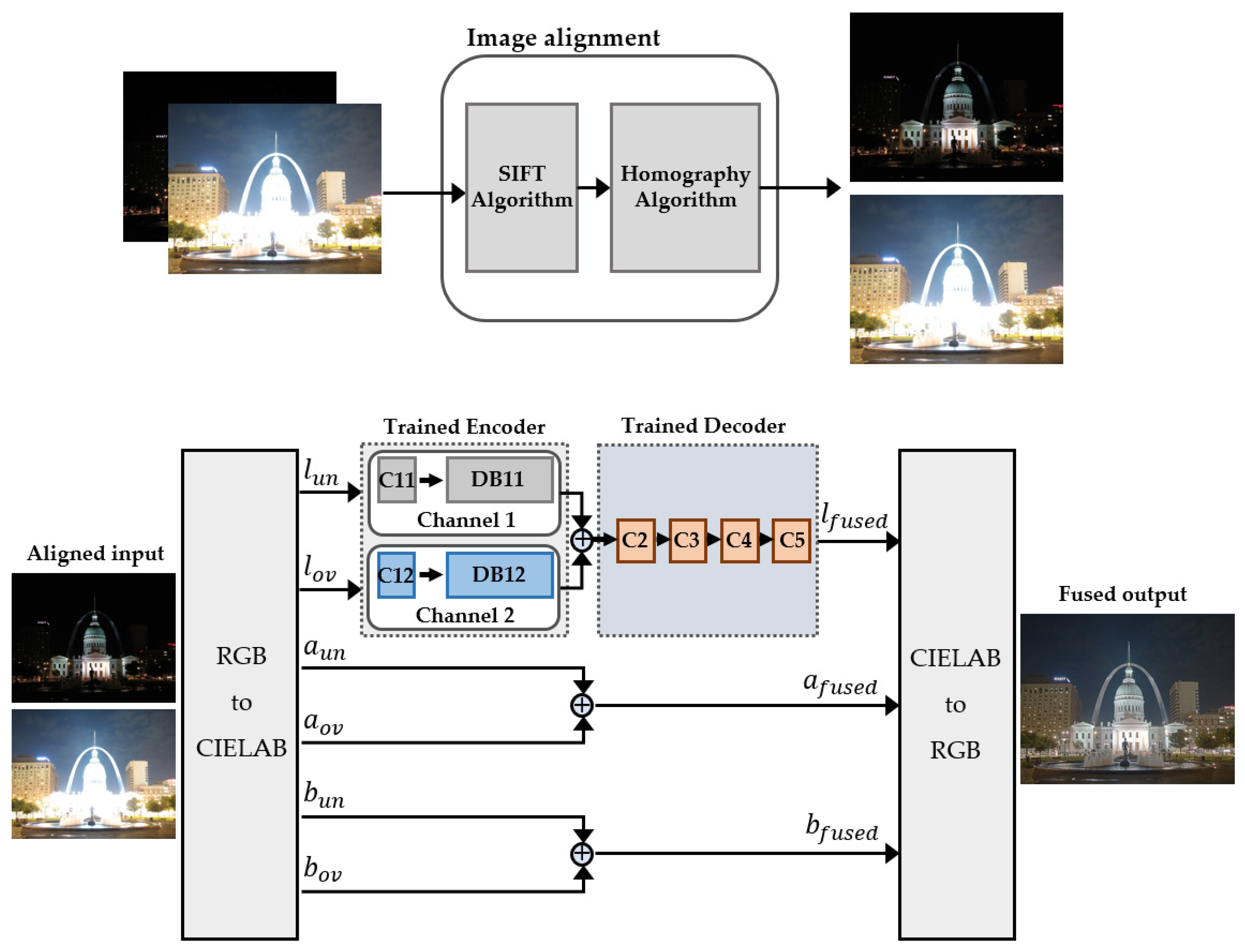
3.6. Image Fusion Process
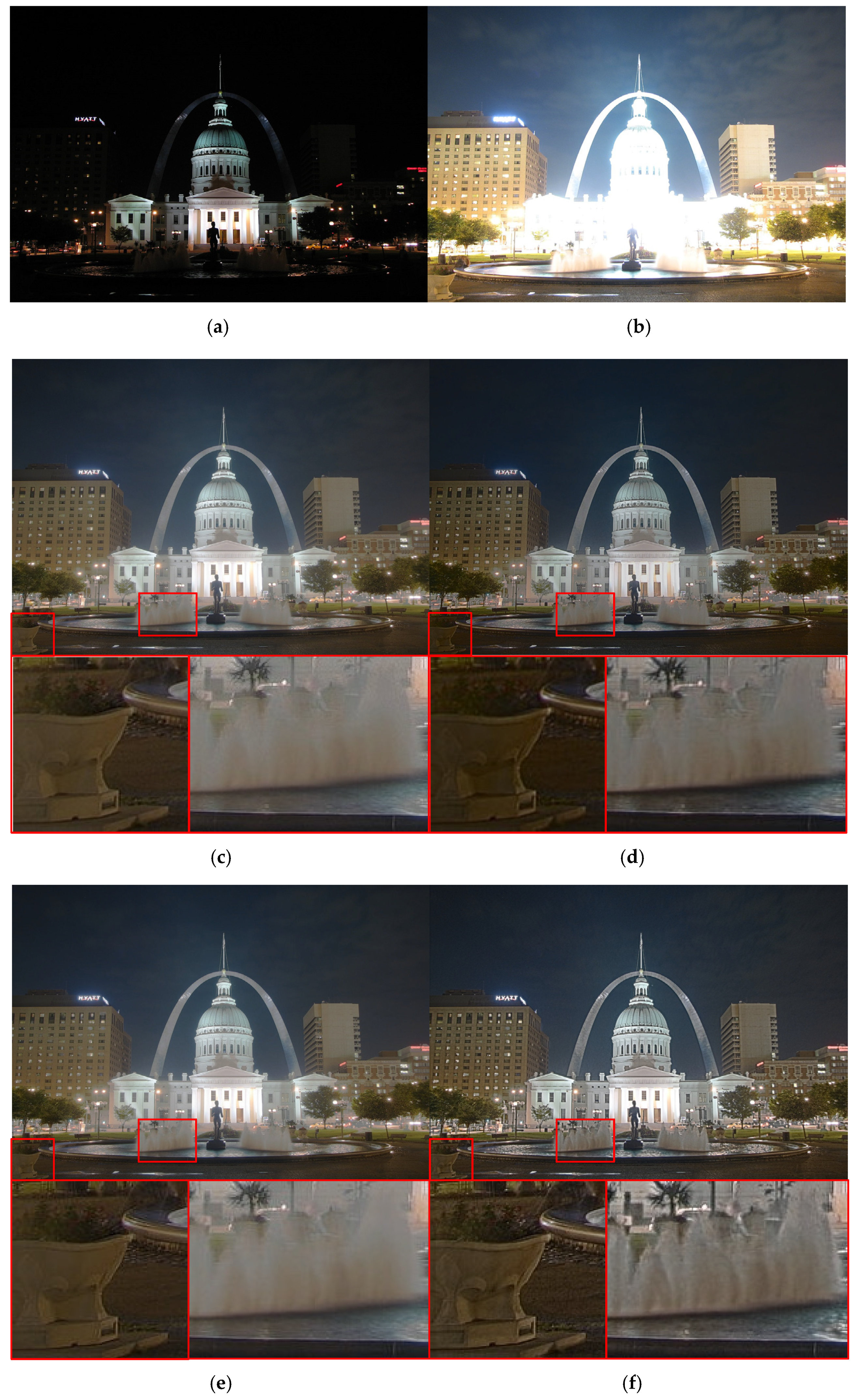
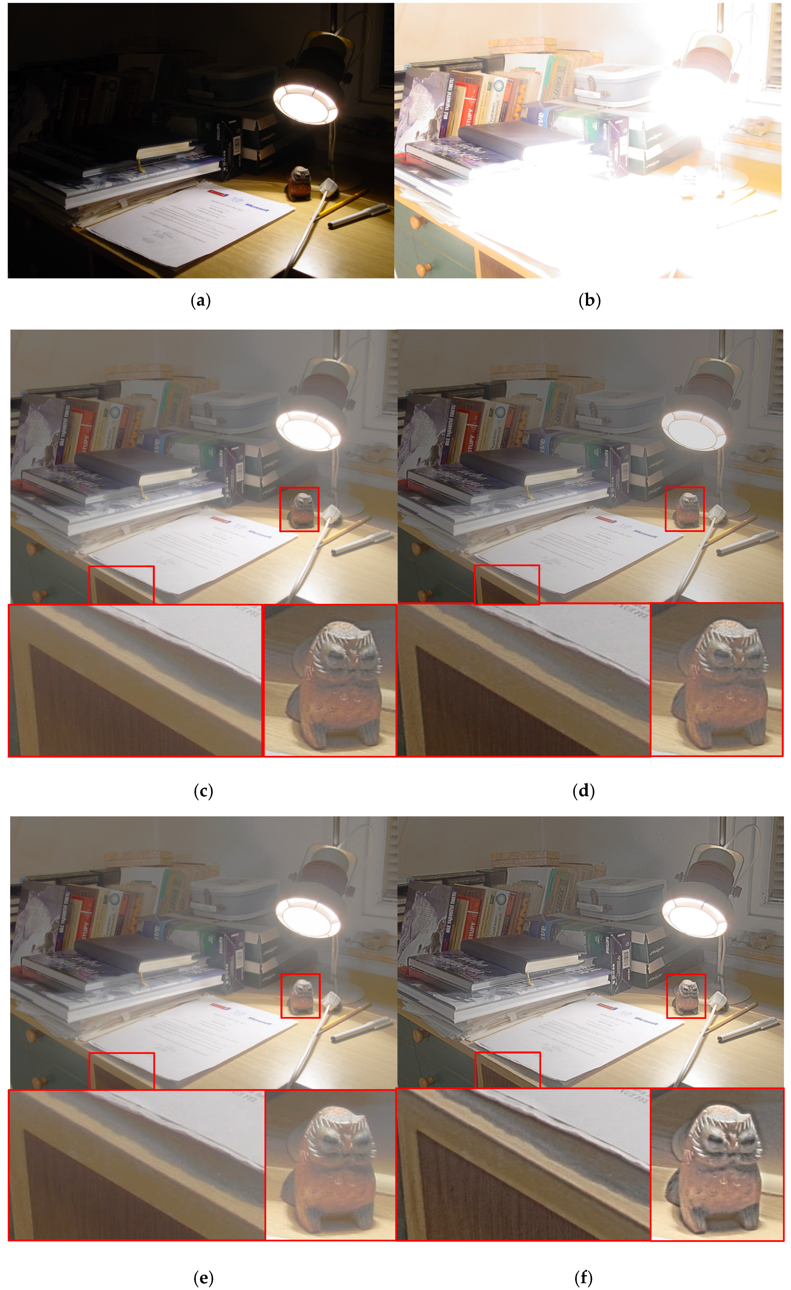
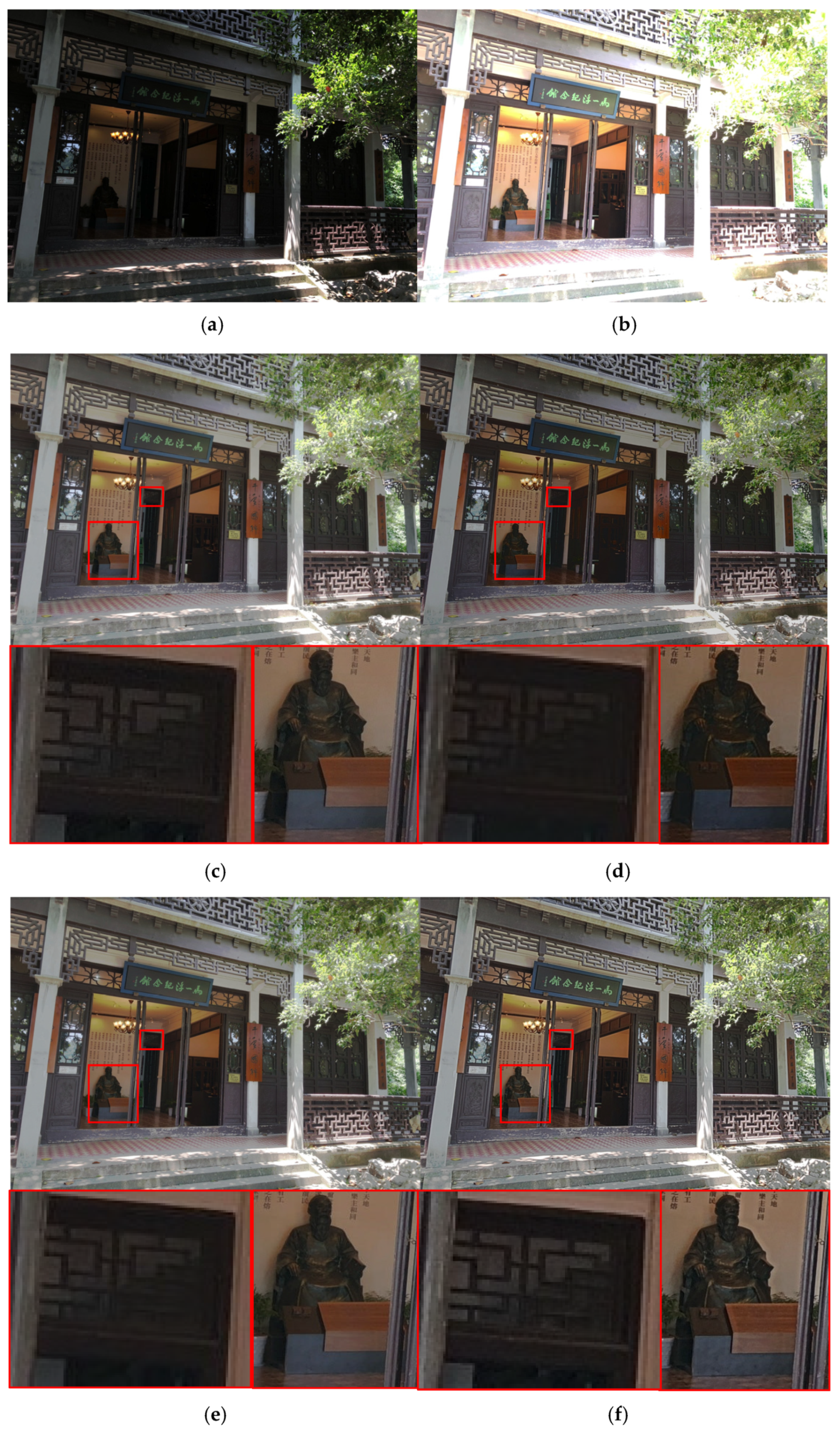
4. Experimental Results
5. Conclusions
Author Contributions
Funding
Data Availability Statement
Conflicts of Interest
References
- Reinhard, E.; Stark, M.; Shirley, P.; Ferwerda, J. Photographic Tone Reproduction for Digital Images. In Proceedings of the SIGGRAPH 2002: 29th Annual Conference on Computer Graphics and Interactive Techniques, San Antonio, TA, USA, 23–26 July 2002; pp. 267–276. [Google Scholar] [CrossRef] [Green Version]
- Duan, J.; Bressan, M.; Dance, C.; Qiu, G. Tone-Mapping High Dynamic Range Images by Novel Histogram Adjustment. Pattern Recognit. 2010, 43, 1847–1862. [Google Scholar] [CrossRef]
- Jung, T.; Kwon, H.J.; Hahn, J.; Lee, S.H. Enhanced HDR Image Reproduction Using Gamma-Adaptation-Based Tone Compression and Detail-Preserved Blending. IEICE Trans. Fundam. Electron. Commun. Comput. Sci. 2020, E103A, 728–732. [Google Scholar] [CrossRef]
- Burt, P.J. The Pyramid as a Structure for Efficient Computation; Springer: Berlin/Heidelberg, Germany, 1984; pp. 6–35. [Google Scholar] [CrossRef]
- Jinno, T.; Okuda, M. Multiple Exposure Fusion for High Dynamic Range Image Acquisition. IEEE Trans. Image Process. 2012, 21, 358–365. [Google Scholar] [CrossRef] [PubMed]
- An, J.; Lee, S.H.; Kuk, J.G.; Cho, N.I. A Multi-Exposure Image Fusion Algorithm without Ghost Effect. In Proceedings of the 2011 IEEE International Conference on Acoustics, Speech and Signal Processing, Prague, Czech Republic, 22–27 May 2011; pp. 1565–1568. [Google Scholar] [CrossRef]
- Li, H.; Wu, X.J. DenseFuse: A Fusion Approach to Infrared and Visible Images. IEEE Trans. Image Process. 2019, 28, 2614–2623. [Google Scholar] [CrossRef] [Green Version]
- Qu, L.; Liu, S.; Wang, M.; Song, Z. TransMEF: A Transformer-Based Multi-Exposure Image Fusion Framework Using Self-Supervised Multi-Task Learning. Proc. AAAI Conf. Artif. Intell. 2022, 36, 2126–2134. [Google Scholar] [CrossRef]
- Bruce, N.D.B. ExpoBlend: Information Preserving Exposure Blending Based on Normalized Log-Domain Entropy. Comput. Graph. 2014, 39, 12–23. [Google Scholar] [CrossRef]
- Song, M.; Tao, D.; Chen, C.; Bu, J.; Luo, J.; Zhang, C. Probabilistic Exposure Fusion. IEEE Trans. Image Process. 2012, 21, 341–357. [Google Scholar] [CrossRef]
- Lee, S.H.; Park, J.S.; Cho, N.I. A Multi-Exposure Image Fusion Based on the Adaptive Weights Reflecting the Relative Pixel Intensity and Global Gradient. In Proceedings of the 2018 IEEE International Conference on Image Processing (ICIP 2018), Athens, Greece, 7–10 October 2018; pp. 1737–1741. [Google Scholar] [CrossRef]
- Xu, F.; Liu, J.; Song, Y.; Sun, H.; Wang, X. Multi-Exposure Image Fusion Techniques: A Comprehensive Review. Remote Sens. 2022, 14, 771. [Google Scholar] [CrossRef]
- Li, S.; Kang, X.; Fang, L.; Hu, J.; Yin, H. Pixel-Level Image Fusion: A Survey of the State of the Art. Inf. Fusion 2017, 33, 100–112. [Google Scholar] [CrossRef]
- Huang, F.; Zhou, D.; Nie, R.; Yu, C. A Color Multi-Exposure Image Fusion Approach Using Structural Patch Decomposition. IEEE Access 2018, 6, 42877–42885. [Google Scholar] [CrossRef]
- Wang, S.; Zhao, Y. A Novel Patch-Based Multi-Exposure Image Fusion Using Super-Pixel Segmentation. IEEE Access 2020, 8, 39034–39045. [Google Scholar] [CrossRef]
- Kalantari, N.K.; Ramamoorthi, R. Deep High Dynamic Range Imaging of Dynamic Scenes. ACM Trans. Graph. 2017, 36, 1–12. [Google Scholar] [CrossRef] [Green Version]
- Xu, H.; Ma, J.; Jiang, J.; Guo, X.; Ling, H. U2Fusion: A Unified Unsupervised Image Fusion Network. IEEE Trans. Pattern Anal. Mach. Intell. 2022, 44, 502–518. [Google Scholar] [CrossRef]
- Prabhakar, K.R.; Srikar, V.S.; Babu, R.V. DeepFuse: A Deep Unsupervised Approach for Exposure Fusion with Extreme Exposure Image Pairs. In Proceedings of the 2017 IEEE International Conference on Computer Vision (ICCV), Venice, Italy, 22–29 October 2017; pp. 4724–4732. [Google Scholar]
- Wang, Z.; Simoncelli, E.P.; Bovik, A.C. Multi-Scale Structural Similarity for Image Quality Assessment. Conf. Rec. Asilomar Conf. Signals Syst. Comput. 2003, 2, 1398–1402. [Google Scholar] [CrossRef] [Green Version]
- Rahman, S.; Rahman, M.M.; Abdullah-Al-Wadud, M.; Al-Quaderi, G.D.; Shoyaib, M. An Adaptive Gamma Correction for Image Enhancement. Eurasip J. Image Video Process. 2016, 2016, 35. [Google Scholar] [CrossRef] [Green Version]
- Lowe, D.G. Distinctive Image Features from Scale-Invariant Keypoints. Int. J. Comput. Vis. 2004, 60, 91–110. [Google Scholar] [CrossRef]
- Sukthankar, R.; Stockton, R.G.; Mullin, M.D. Smarter Presentations: Exploiting Homography in Camera-Projector Systems. Proc. IEEE Int. Conf. Comput. Vis. 2001, 1, 247–253. [Google Scholar] [CrossRef]
- Son, D.-M.; Kwon, H.-J.; Lee, S.-H. Visible and Near Infrared Image Fusion Using Base Tone Compression and Detail Transform Fusion. Chemosensors 2022, 10, 124. [Google Scholar] [CrossRef]
- Debevec, P.E.; Malik, J. Recovering High Dynamic Range Radiance Maps from Photographs. In Proceedings of the ACM SIGGRAPH 2008 Classes, Los Angeles, CA, USA, 11–15 August 2008; Volume 31. [Google Scholar] [CrossRef]
- HDRsoft Gallery. Available online: http://www.hdrsoft.com/examples2.html (accessed on 26 November 2015).
- Cai, J.; Gu, S.; Zhang, L. Learning a Deep Single Image Contrast Enhancer from Multi-Exposure Images. IEEE Trans. Image Process. 2018, 27, 2049–2062. [Google Scholar] [CrossRef]
- Multi-Exposure HDR Capture. Wikipedia. Available online: https://en.wikipedia.org/wiki/Multi-exposure_HDR_capture (accessed on 3 January 2023).
- Cui, G.; Feng, H.; Xu, Z.; Li, Q.; Chen, Y. Detail Preserved Fusion of Visible and Infrared Images Using Regional Saliency Extraction and Multi-Scale Image Decomposition. Opt. Commun. 2015, 341, 199–209. [Google Scholar] [CrossRef]
- Rajalingam, B.; Priya, R. Hybrid Multimodality Medical Image Fusion Technique for Feature Enhancement in Medical Diagnosis. Int. J. Eng. Sci. Invent. 2018, 2, 52–60. [Google Scholar]
- Haghighat, M.; Razian, M.A. Fast-FMI: Non-Reference Image Fusion Metric. In Proceedings of the 2014 IEEE 8th International Conference on Application of Information and Communication Technologies (AICT), Astana, Kazakhstan, 15–17 October 2014; pp. 1–3. [Google Scholar]
- Hassen, R.; Wang, Z.; Salama, M.M.A. Image Sharpness Assessment Based on Local Phase Coherence. IEEE Trans. Image Process. 2013, 22, 2798–2810. [Google Scholar] [CrossRef] [PubMed]
- Vu, C.T.; Phan, T.D.; Chandler, D.M. S3: A Spectral and Spatial Measure of Local Perceived Sharpness in Natural Images. IEEE Trans. Image Process. 2012, 21, 934–945. [Google Scholar] [CrossRef] [PubMed]
- Eskicioglu, A.M.; Fisher, P.S. Image Quality Measures and Their Performance. IEEE Trans. Commun. 1995, 43, 2959–2965. [Google Scholar] [CrossRef] [Green Version]
- Venkatanath, N.; Praneeth, D.; Maruthi Chandrasekhar, B.H.; Channappayya, S.S.; Medasani, S.S. Blind Image Quality Evaluation Using Perception Based Features. In Proceedings of the 2015 21st National Conference on Communications (NCC 2015), Mumbai, India, 27 February–1 March 2015. [Google Scholar] [CrossRef] [Green Version]
- Xydeas, C.S.; Petrović, V. Objective Image Fusion Performance Measure. Electron. Lett. 2000, 36, 308. [Google Scholar] [CrossRef] [Green Version]
- Han, Y.; Cai, Y.; Cao, Y.; Xu, X. A New Image Fusion Performance Metric Based on Visual Information Fidelity. Inf. Fusion 2013, 14, 127–135. [Google Scholar] [CrossRef]


| Method | AG | EI | FMI | LPC-SI | S3 | SF | PIQE | MS-SSIM | Qabf | VIFF |
|---|---|---|---|---|---|---|---|---|---|---|
| DenseFuse | 4.1796 | 41.3714 | 0.3366 | 0.9369 | 0.1830 | 13.7378 | 26.0896 | 0.8781 | 0.4208 | 0.4285 |
| U2Fusion | 4.7719 | 48.9770 | 0.2891 | 0.9438 | 0.1798 | 15.3116 | 35.4318 | 0.8468 | 0.3898 | 0.4181 |
| TransMEF | 3.9983 | 40.3294 | 0.2910 | 0.9360 | 0.1627 | 13.1360 | 37.8373 | 0.8636 | 0.3520 | 0.4084 |
| HyperP_MB | 6.1319 | 61.6277 | 0.3447 | 0.9543 | 0.2369 | 19.7974 | 25.8651 | 0.8916 | 0.5059 | 0.5477 |
| Co-Target | MB | PT | AG | EI | FMI | LPC-SI | S3 | SF | PIQE | MS-SSIM | Qabf | VIFF |
|---|---|---|---|---|---|---|---|---|---|---|---|---|
| ✓ | 4.8802 | 49.2164 | 0.3491 | 0.9526 | 0.2021 | 16.0696 | 27.4676 | 0.8809 | 0.4622 | 0.4604 | ||
| ✓ | ✓ | 5.9602 | 60.0486 | 0.3459 | 0.9549 | 0.2294 | 19.3997 | 27.9720 | 0.8962 | 0.5184 | 0.5421 | |
| ✓ | ✓ | ✓ | 6.1319 | 61.6277 | 0.3447 | 0.9543 | 0.2369 | 19.7974 | 25.8651 | 0.8916 | 0.5059 | 0.5477 |
Disclaimer/Publisher’s Note: The statements, opinions and data contained in all publications are solely those of the individual author(s) and contributor(s) and not of MDPI and/or the editor(s). MDPI and/or the editor(s) disclaim responsibility for any injury to people or property resulting from any ideas, methods, instructions or products referred to in the content. |
© 2023 by the authors. Licensee MDPI, Basel, Switzerland. This article is an open access article distributed under the terms and conditions of the Creative Commons Attribution (CC BY) license (https://creativecommons.org/licenses/by/4.0/).
Share and Cite
Im, C.-G.; Son, D.-M.; Kwon, H.-J.; Lee, S.-H. Multi-Task Learning Approach Using Dynamic Hyperparameter for Multi-Exposure Fusion. Mathematics 2023, 11, 1620. https://doi.org/10.3390/math11071620
Im C-G, Son D-M, Kwon H-J, Lee S-H. Multi-Task Learning Approach Using Dynamic Hyperparameter for Multi-Exposure Fusion. Mathematics. 2023; 11(7):1620. https://doi.org/10.3390/math11071620
Chicago/Turabian StyleIm, Chan-Gi, Dong-Min Son, Hyuk-Ju Kwon, and Sung-Hak Lee. 2023. "Multi-Task Learning Approach Using Dynamic Hyperparameter for Multi-Exposure Fusion" Mathematics 11, no. 7: 1620. https://doi.org/10.3390/math11071620