Mean Square Exponential Stability of Stochastic Delay Differential Systems with Logic Impulses

Abstract

This paper focuses on the mean square exponential stability of stochastic delay differential systems with logic impulses. Firstly, a class of nonlinear stochastic delay differential systems with logic impulses is constructed. Then, the logic impulses are transformed into an equivalent algebraic expression by using the semi-tensor product method. Thirdly, the mean square exponential stability criteria of nonlinear stochastic delay differential systems with logic impulses are given. Finally, two kinds of stochastic delay differential systems with logic impulses and uncertain parameters are discussed, and the coefficient conditions guaranteeing the mean square exponential stability of these systems are obtained.

1. Introduction

Stochastic differential systems are widely used in many fields, such as physics, biology, economics and finance. For example, option pricing in the financial economy, wide-area security in the electrical power system, and mechanisms of tumor evolution in biology, etc. can be well analyzed and controlled by stochastic differential systems. In recent years, the stability problems of stochastic systems have received extensive attention, such as in [1,2,3] and references therein. Furthermore, the research of stochastic delay systems has also been developed rapidly, such as [4,5,6,7,8] and references therein. On the other hand, the impulsive effects are widely encountered in engineering application areas and natural systems, so stochastic systems with impulsive effects have always been one of the focused issues in research, such as [9,10,11,12,13,14,15,16,17] and references therein.

Meanwhile, the study of hybrid systems, including logics developed rapidly (see [18,19,20,21,22,23,24,25,26] and references therein) after the semi-tensor product method was proposed in [18]. In recent years, the impulsive effects suffered by logic choices have attracted the attention of some researchers, such as [27,28,29,30,31]. As far as we know, few studies have been done on stochastic systems with logic impulses. To date, only [30] has constructed a class of scalar linear stochastic delay differential systems with logic impulses and analyzed their stability in published papers. Therefore, it is necessary to construct and analyze more general stochastic delay differential systems with logic impulses.

It is widely known that the Lyapunov function and It$\widehat{o}$’s formula are common traditional methods used to study the stability of stochastic systems. However, the It$\widehat{o}$ formula cannot be used effectively in stochastic delay differential systems with logic impulses since it is difficult to integrate the equation over the interval containing the impulsive points. At the same time, it is not easy to construct Lyapunov functions from stochastic differential equations, and most of the results are given in terms of matrix inequalities or differential inequalities which are not easy to apply in practice, see [5,6,32,33]. Therefore, we aim to give some stability criteria for stochastic delay differential systems with logic impulses that can overcome the above two difficulties, i.e., relatively easy to verify.

In view of the above considerations, we think that it is meaningful to construct a stochastic delay differential system with logic impulses and give its stability criteria which are not involved in Lyapunov functions and are relatively easy to verify. The main purpose and work of this paper can be concluded as follows: (i) Construct a class of nonlinear stochastic delay differential systems with logic impulses. (ii) By constructing a nonlinear transformation, the connection between stochastic delay differential systems with logic impulses and non-impulsive stochastic delay differential systems is established. Thus, the difficulty that It$\widehat{o}$ formula cannot be integrated at the impulsive points are overcome. (iii) Obtained some stability criteria. It is worth noting that the stability criteria do not require the construction of Lyapunov functions. (iv) The stability results are applied to two kinds of stochastic delay differential systems with logic impulses and uncertain parameters, and the coefficient conditions ensuring the mean square exponential stability of these systems are obtained.

This paper is organized as follows: In Section 2, some basic concepts and lemmas are collected. In Section 3, a class of n-dimensional nonlinear stochastic delay differential systems with logic impulses is constructed, and the logic impulses are transformed into an equivalent algebraic expression by using the semi-tensor product method. Then, the stability of the nonlinear stochastic delay differential systems with logic impulses is studied, and some stability criteria, especially the mean square exponential stability criteria are obtained in Section 4. In Section 5, two kinds of stochastic delay differential systems with logic impulses and uncertain parameters are discussed, and the coefficient conditions guaranteeing the mean square exponential stability of these systems are obtained. Lastly, a discussion is given in Section 6.

2. Preliminaries

Let $\{\Omega ,F,{\left\{F_t\right\}}_{t\ge 0},P\}$ be a complete probability space with a filtration ${\left\{F_t\right\}}_{t\ge 0}$ satisfying the usual conditions (i.e., right continuous and $F_0$ containing all p-null sets). Let $w\left(t\right)={(w_1\left(t\right),w_2\left(t\right),\cdots ,w_m\left(t\right))}^T$ be an m-dimensional Brownian motion defined on $\{\Omega ,F,{\left\{F_t\right\}}_{t\ge 0},P\}$, $E\xi$ denotes the expectation of stochastic process $\xi$, and $\parallel ·\parallel$ denotes the Euclidean norm on $R^n$. Let $C([t_0-r,t_0],R^n)$ denote the Banach space of all functions which are real-valued absolutely continuous on $[t_0-r,t_0]$, with the norm $\parallel \xi \parallel =\underset{t_0-r\le s\le t_0}{sup}\parallel \xi \left(s\right)\parallel$. Let $C_{F_0}^b([t_0-r,t_0],R^n)$ denotes the family of $F_{t_0}$-measurable bounded $C([t_0-r,t_0],R^n)$-valued random variables, satisfying $\underset{t_0-r\le s\le t_0}{sup}E{\parallel \varphi \parallel }^p<\infty$.

Let $A={\left(a_{ij}\right)}_{n\times m}$ and $B={\left(b_{ij}\right)}_{n\times m}$ be two $n\times m$ matrices, $R^{n\times m}$ denotes the set of all $n\times m$ matrices. In this paper, $A\ge B$ means that $a_{ij}\ge b_{ij}$, $i=1,2,\cdots ,n$, $j=1,2,\cdots ,m$. In particular, $A\ge 0$ means that $a_{ij}\ge 0$, $i=1,2,\cdots ,n$, $j=1,2,\cdots ,m$, and $R_{+}^{n\times m}$ denotes the set of all nonnegative $n\times m$ matrices. $A\gg B$ means that $a_{ij}>b_{ij}$, $i=1,2,\cdots ,n$, $j=1,2,\cdots ,m$. In particular, $A\gg 0$ means that $a_{ij}>0$, and $A\ll 0$ means that $a_{ij}<0$, $i=1,2,\cdots ,n$, $j=1,2,\cdots ,m$. A matrix $A={\left(a_{ij}\right)}_{n\times n}\in R^{n\times n}$ is called a Metzler matrix, if its off-diagonal elements are all non-negative, i.e. $a_{ij}\ge 0,i\ne j.$ A matrix $A\in R^{n\times n}$ is said to be Hurwitz stable, if $max\{\Re z:\det (z{I}_n-A)=0\}<0$.

Let ${\delta }_n^i$ denotes the ith column of the identity matrix $I_n$, $i=1,2,\cdots ,n$, and ${\Delta }_n=\left\{{\delta }_n^i\right|i=1,2,\cdots ,n\}$. A matrix $L\in R^{n\times m}$ is called logical matrix, if $Col\left(L\right)\subset {\Delta }_n$. Let ${\mathcal{L}}_{n\times m}$ denotes the set of all $n\times m$ logical matrices. For a logical matrix $L\in {\mathcal{L}}_{m\times n}$, $L=({\delta }_m^{i_1},{\delta }_m^{i_2},\cdots ,{\delta }_m^{i_n})$ is denoted by $L={\delta }_m(i_1,i_2,\cdots ,i_n)$ for simplicity. $D=\{0,1\}$ denotes the family of logical values. Moreover, we identify logical values with equivalent vectors as: $T=1\sim {\delta }_2^1$, $F=0\sim {\delta }_2^2$.

The Hadamard product and the Kronecker product of matrices are two kinds of classical matrix operations. In this paper, ${}^{\prime }{\circ }^{\prime }$ represents the Hadamard product of matrices, and ${}^{\prime }{\otimes }^{\prime }$ represents the Kronecker product of matrices. Furthermore, for two matrices $A\in R^{n\times m}$ and $B\in R^{p\times q}$, the semi-tensor product of A and B is: $A⋉B=(A\otimes I_{\alpha /m})(B\otimes I_{\alpha /p}),$ where $\alpha =lcm(m,p)$ denotes the least common multiple of m and p, see [18]. When $m=p$, the semi-tensor product degenerates into the traditional matrix product.

Lemma 1 

(see [27]). Given a logical function $f(p_1,p_2,\cdots ,p_r)\in {\Delta }_2$ with logical variables $p_1,p_2,\cdots ,p_r\in {\Delta }_2$, there exists a unique $2\times 2^r$ logical matrix $M_f$ called the structure matrix of f, such that

$$f(p_1,p_2,\cdots ,p_r)=M_f⋉p_1⋉p_2⋉\cdots ⋉p_r=M_f{⋉}_{i=1}^r{p}_i$$

Moreover, $Col\left(M_f\right)\subset {\Delta }_2$. We note that ${⋉}_{i=1}^r{p}_i\in {\Delta }_{2^r}$.

Lemma 2 

(see [6]). Let matrix $A\in R^{n\times n}$ be a Metzler matrix. Then, A is Hurwitz stable if, and only if, $Ap\ll 0$ for some $p\in R_{+}^n$, $p\gg 0$.

3. Stochastic Delay Differential Systems with Logic Impulses Model

Consider the following nonlinear stochastic delay differential systems with logic impulses:

$$\left\{\begin{array}{cc}dy\left(t\right)=f(t,y\left(t\right),y(t-h\left(t\right)))dt+g(t,y\left(t\right),y(t-\tau \left(t\right)))dw\left(t\right),\hfill & t\ge t_0,t\ne t_k\hfill \\ \Delta y\left(t_k\right)={\Psi }_k\left(y\left(t_k\right)\right),\hfill & k\in N\hfill \end{array}\right.$$

(1)

with the initial condition:

$$y\left(t\right)=\xi \left(t\right),t\in [t_0-r,t_0]$$

(2)

where the fixed impulsive points ${\left\{t_k\right\}}_{k=1}^{\infty }$ satisfying $0\le t_0<t_1<\cdots <t_k<\cdots$, and $\underset{k\to \infty }{lim}{t}_k=\infty$, $y\left(t\right)={(y_1\left(t\right),\cdots ,y_n\left(t\right))}^T$, $\Delta y\left(t\right)={(\Delta y_1\left(t\right),\cdots ,\Delta y_n\left(t\right))}^T$, $\xi \in C_{F_{t_0}}^b([t_0-r,t_0],R^n)$, $f:R_{+}\times R^n\times R^n\to R^n$ and $g:R_{+}\times R^n\times R^n\to R^{n\times m}$ are measurable continuous functions, $f(t,0,0)\equiv 0$ and $g(t,0,0)\equiv 0$ for any $t\ge t_0$, $h\left(t\right)\in C\left(\right[0,+\infty ),[0,h\left]\right)$, $\tau \left(t\right)\in C\left(\right[0,+\infty ),[0,\tau \left]\right)$, here $h=\underset{t\ge t_0}{sup}h\left(t\right)$, $\tau =\underset{t\ge t_0}{sup}\tau \left(t\right)$, $r=max\{h,\tau \}$.

The logic impulses ${\Psi }_k\left(y\left(t_k\right)\right)$, which are affected by the logical relationship between $y_i\left(t_k\right)$, $i=1,2,\cdots ,n$, can be described as follows:

$$\begin{array}{c}\hfill \Delta y_i\left(t_k\right)=y_i\left(t_k^{+}\right)-y_i\left(t_k\right)=u_i\left(t_k\right)I_k\left(y_i\left(t_k\right)\right)+\overline{u_i\left(t_k\right)}{J}_k\left(y_i\left(t_k\right)\right).\end{array}$$

where, for $\forall k\in N$, continuous function $I_k$ and $J_k$ satisfy $I_k\left(0\right)=J_k\left(0\right)=0$. And for $\forall s\in R$, $s\ne 0$, $I_k\left(s\right)\ne -s$, $J_k\left(s\right)\ne -s$. $u_i:{\{{\delta }_2^1,{\delta }_2^2\}}^n\to \{0,1\}$ is a logical function related to $y_1\left(t\right),y_2\left(t\right),\cdots ,y_n\left(t\right)$, and ${\overline{u}}_i$ denotes the negation logical function of $u_i$, can be expressed as follows:

$$u_i\left(t\right)=u_i(p_1\left(y_1\left(t\right)\right),\cdots ,p_n\left(y_n\left(t\right)\right)),\overline{u_i\left(t\right)}=\overline{u_i(p_1\left(y_1\left(t\right)\right),\cdots ,p_n\left(y_n\left(t\right)\right))}.$$

The piecewise logical function $p_i:R\to \{0,1\}$ is defined as follows:

$$p_i\left(s\right)=\left\{\begin{array}{c}{\delta }_2^2\sim 0,\left|q_i\left(s\right)\right|\ge c_i,\hfill \\ {\delta }_2^1\sim 1,\left|q_i\left(s\right)\right|<c_i.\hfill \end{array}\right.$$

where, $q_i\in C(R,R)$, $c_i>0$ is the threshold.

Then, the impulses will be selected from $I_k$ and $J_k$ based on the values of the logical functions $u_i$ and ${\overline{u}}_i$. It is also assumed that for a given initial function $\xi \in C_{F_{t_0}}^b([t_0-r,t_0],R^n)$, systems (1)–(2) always has a unique solution in this paper.

Next, by using the method of semi-tensor product, we transform the impulses that contain logical functions in system (1) into algebraic expressions. Because $u_i$ and ${\overline{u}}_i$ are logical functions, and ${\overline{u}}_i$ is the negation logical function of $u_i$, the logical impulse effect can be expressed in the following form:

$$\begin{array}{c}\hfill \Delta y_i\left(t_k\right)=[I_k\left(y_i\left(t_k\right)\right),J_k\left(y_i\left(t_k\right)\right)]L_i(p_1\left(y_1\left(t_k\right)\right),\cdots ,p_n\left(y_n\left(t_k\right)\right)),\end{array}$$

where, $L_i:{\{{\delta }_2^1,{\delta }_2^2\}}^n\to \{{\delta }_2^1,{\delta }_2^2\}$ is logical function. According to Lemma 1, there exists a unique $2\times 2^n$ structural matrix $M_i$ such that

$$L_i(p_1\left(y_1\left(t_k\right)\right),\cdots ,p_n\left(y_n\left(t_k\right)\right))=M_i{⋉}_{i=1}^n{p}_i\left(y_i\left(t_k\right)\right)$$

Let $p\left(y\left(t_k\right)\right):={⋉}_{i=1}^n{p}_i\left(y_i\left(t_k\right)\right)$, thus $p\left(y\left(t_k\right)\right)\in {\Delta }_{2^n}$.

Thus, the logic impulses of system (1) can be described by the following algebraic expression:

$$\begin{array}{c}\hfill \Delta y_i\left(t_k\right)=[I_k\left(y_i\left(t_k\right)\right),J_k\left(y_i\left(t_k\right)\right)]M_{i}p\left(y\left(t_k\right)\right):={\varphi }_k\left(y_i\left(t_k\right)\right)M_{i}p\left(y\left(t_k\right)\right),\end{array}$$

or

$$\begin{array}{cc}\hfill \Delta y\left(t_k\right)& ={\Psi }_k\left(y\left(t_k\right)\right):={\mathsf{\Phi }}_k\left(y\left(t_k\right)\right)Mp\left(y\left(t_k\right)\right),\hfill \end{array}$$

where, ${\varphi }_k\left(y_i\left(t_k\right)\right)=[I_k\left(y_i\left(t_k\right)\right),J_k\left(y_i\left(t_k\right)\right)]$, $M={[M_1^T,M_2^T,\cdots ,M_n^T]}^T\in R^{2n\times 2^n},$

$$\begin{array}{cc}\hfill {\mathsf{\Phi }}_k\left(y\left(t_k\right)\right)& =diag({\varphi }_k\left(y_1\left(t_k\right)\right),{\varphi }_k\left(y_2\left(t_k\right)\right),\dots ,{\varphi }_k\left(y_n\left(t_k\right)\right))\hfill \\ \hfill & ={\left(\begin{array}{cccc}{I}_k\left(y_1\left(t_k\right)\right)& J_k\left(y_1\left(t_k\right)\right)& & \\ & \ddots & & \\ & & I_k\left(y_n\left(t_k\right)\right)& J_k\left(y_n\left(t_k\right)\right)\end{array}\right)}_{n\times 2n}.\hfill \end{array}$$

Now, the nonlinear stochastic delay differential system with logic impulses (1)–(2) can be expressed as follows:

$$\left\{\begin{array}{cc}d{y}_i\left(t\right)=f_i(t,y\left(t\right),y(t-h\left(t\right)))dt+\sum _{j=1}^m{g}_{ij}(t,y\left(t\right),y(t-\tau \left(t\right)))d{w}_j\left(t\right),\hfill & t\ge t_0,t\ne t_k\hfill \\ \Delta y_i\left(t_k\right)={\varphi }_k\left(y_i\left(t_k\right)\right)M_{i}p\left(y\left(t_k\right)\right),\hfill & k\in N\hfill \end{array}\right.$$

(3)

or

$$\left\{\begin{array}{cc}dy\left(t\right)=f(t,y\left(t\right),y(t-h\left(t\right)))dt+g(t,y\left(t\right),y(t-\tau \left(t\right)))dw\left(t\right),\hfill & t\ge t_0,t\ne t_k\hfill \\ \Delta y\left(t_k\right)={\mathsf{\Phi }}_k\left(y\left(t_k\right)\right)Mp\left(y\left(t_k\right)\right),\hfill & k\in N\hfill \end{array}\right.$$

(4)

where $f={(f_1,\cdots ,f_n)}^T\in R^n$, $g={\left(g_{ij}\right)}_{n\times m}\in R^{n\times m}$, $i=1,2,\cdots ,n$.

Definition 1 

(see [30]). A function $y\left(t\right)={(y_1\left(t\right),\cdots ,y_n\left(t\right))}^T$ is called a solution of (1)–(2) on $[t_0-r,\infty )$, if

(i) $y_i\left(t\right)$ is absolutely continuous on each interval $(t_{k-1},t_k]$, $k\in N$.

(ii) For any $t_k$, $k\in N$, $y_i\left(t_k^{+}\right)$ and $y_i\left(t_k^{-}\right)$ exist, and $y\left(t_k^{-}\right)=y\left(t_k\right)$.

(iii) $y\left(t\right)$ satisfies the differential Equation (1) almost everywhere on $[t_0,+\infty )\setminus {\left\{t_k\right\}}_{k\in N}$ and the impulsive condition at every $t_k$, $k\in N$.

(iv) $y\left(t\right)$ satisfies the initial condition (2) on $[t_0-r,t_0]$.

Obviously, system (1) admits a trivial solution $y\left(t\right)\equiv 0$. Throughout this paper, we assume that any solution $y\left(t\right)={(y_1\left(t\right),\cdots ,y_n\left(t\right))}^T$ of system (1) in addition to the zero solution satisfies $y_i\left(t_k\right)\ne 0$, $i=1,2,\cdots ,n$.

Definition 2 

(see [30]). The trivial solution of (1)–(2) is said to be mean square exponentially stable if there exist a pair of positive constants λ and K such that,

$${E\parallel y\left(t\right)\parallel }^2\le K{e}^{-\lambda (t-t_0)}E{\parallel \xi \parallel }^2,t\ge t_0,$$

for any initial function $\xi \left(t\right)\in C_{F_0}^b([t_0-r,t_0],R^n)$.

4. Stability Criteria

In this section, by constructing a nonlinear transformation, the relation between a stochastic delay differential system with logic impulses and a stochastic delay differential system without impulses is established, and some stability criteria are given.

Introduce the following functions:

$${\alpha }_i\left(t\right)=\prod _{t_0\le t_k<t}\frac{y_i\left(t_k\right)}{y_i\left(t_k\right)+{\varphi }_k\left(y_i\left(t_k\right)\right)M_{i}p\left(y\left(t_k\right)\right)},$$

for $i=1,2,\cdots ,n$. If the number of factors in a product is zero, we set the product to be equal to 1. Let $\alpha \left(t\right)={({\alpha }_1\left(t\right),{\alpha }_2\left(t\right),\cdots ,{\alpha }_n\left(t\right))}^T\in R^n$, and ${\alpha }^{-1}\left(t\right)={({\alpha }_1^{-1}\left(t\right),\cdots ,{\alpha }_n^{-1}\left(t\right))}^T\in R^n$. It can be seen that, ${\alpha }_i\left(t\right)$ is a piecewise constant function, so $\dot{{\alpha }_i}\left(t\right)=0$, $i=1,2,\cdots ,n$, is hold almost everywhere on the interval $[t_0-r,\infty )$.

By now, a stochastic delay differential system without impulses can be proposed as follows:

$$\begin{array}{cc}\hfill d{x}_i\left(t\right)=& {\alpha }_i\left(t\right)f_i(t,x\left(t\right)\circ {\alpha }^{-1}\left(t\right),x(t-h\left(t\right))\circ {\alpha }^{-1}(t-h\left(t\right)))dt\hfill \\ \hfill & +{\alpha }_i\left(t\right)\sum _{j=1}^m{g}_{ij}(t,x\left(t\right)\circ {\alpha }^{-1}\left(t\right),x(t-\tau \left(t\right))\circ {\alpha }^{-1}(t-\tau \left(t\right)))d{w}_j\left(t\right),\hfill \end{array}$$

(5)

for $t\ge t_0$, $i=1,2,\cdots ,n$. Or

$$\begin{array}{cc}\hfill dx\left(t\right)=& \tilde{f}(t,x\left(t\right)\circ {\alpha }^{-1}\left(t\right),x(t-h\left(t\right))\circ {\alpha }^{-1}(t-h\left(t\right)))dt\hfill \\ \hfill & +\tilde{g}(t,x\left(t\right)\circ {\alpha }^{-1}\left(t\right),x(t-\tau \left(t\right))\circ {\alpha }^{-1}(t-\tau \left(t\right)))dw\left(t\right),\hfill \end{array}$$

(6)

where $\tilde{f}=\alpha \circ f={({\alpha }_1{f}_1,\cdots ,{\alpha }_n{f}_n)}^T:={({\tilde{f}}_1,\cdots ,{\tilde{f}}_n)}^T\in R^n$, $\tilde{g}={\alpha }^{★}\circ g={\left({\alpha }_i{g}_{ij}\right)}_{n\times m}:={\left({\tilde{g}}_{ij}\right)}_{n\times m}\in R^{n\times m}$, ${\alpha }^{★}:={(\alpha ,\alpha ,\cdots ,\alpha )}_{n\times m}\in R^{n\times m}$.

The initial condition for (5) or (6) is defined by

$$x\left(t\right)=\xi \left(t\right),t\in [t_0-r,t_0]$$

(7)

An absolutely continuous function $x\left(t\right)$ is called a solution of systems (5)–(7), if $x\left(t\right)$ satisfies system (5) almost everywhere on the interval $[t_0-r,\infty )$, and satisfies initial conditions (7). Similar to Definition 2, the definition of mean square exponential stability for systems (5)–(7) can be given, which is omitted here.

System (1) is a hybrid system, which suffers from time-delay effects, impulsive effects, stochastic effects and logic effects simultaneously. It is very difficult to make a qualitative analysis of it directly. By applying the semi-tensor product method and introducing the piecewise constant function $\alpha \left(t\right)$, we construct system (5) with only time delay and stochastic effects, which is much simpler than system (1). Therefore, we aim to get some properties of system (1) through the study of system (5), and provide an effective and feasible method for the study of system (1).

Lemma 3. 

(i) if $x\left(t\right)$ is a solution of (5)–(7), then $y\left(t\right)={\alpha }^{-1}\left(t\right)\circ x\left(t\right)$ is a solution of (1)–(2) on $[t_0-r,+\infty )$.

(ii) if $y\left(t\right)$ is a solution of (1)–(2), then $x\left(t\right)=\alpha \left(t\right)\circ y\left(t\right)$ is a solution of (5)–(7) on $[t_0-r,+\infty )$.

Proof of Lemma 3. 

Step 1. We give the proof of conclusion (i).

Let $x\left(t\right)={(x_1\left(t\right),x_2\left(t\right),\cdots ,x_n\left(t\right))}^T$ be a possible solution of systems (5)–(7), so that $y_i\left(t\right)={\alpha }_i^{-1}\left(t\right)x_i\left(t\right)$, $i=1,2,\cdots ,n$, is absolutely continuous on each interval $(t_{k-1},t_k)\subset [t_0,\infty )$, $k\in N$. Further, because ${\alpha }_i\left(t\right)$, $i=1,2,\cdots ,n$, is a piecewise constant function, for any $t\ne t_k$, we have

$$\begin{array}{cc}\hfill d{y}_i\left(t\right)=& d\left({\alpha }_i^{-1}\left(t\right)x_i\left(t\right)\right)\hfill \\ \hfill =& {\alpha }_i^{-1}\left(t\right)d\left(x_i\left(t\right)\right)\hfill \\ \hfill =& f_i(t,x\left(t\right)\circ {\alpha }^{-1}\left(t\right),x(t-h\left(t\right))\circ {\alpha }^{-1}(t-h\left(t\right)))dt\hfill \\ \hfill & +\sum _{j=1}^m{g}_{ij}(t,x\left(t\right)\circ {\alpha }^{-1}\left(t\right),x(t-\tau \left(t\right))\circ {\alpha }^{-1}(t-\tau \left(t\right)))d{w}_j\left(t\right)\hfill \\ \hfill =& f_i(t,y\left(t\right),y(t-h\left(t\right)))dt+\sum _{j=1}^m{g}_{ij}(t,y\left(t\right),y(t-\tau \left(t\right)))d{w}_j\left(t\right)\hfill \end{array}$$

Thus, $y\left(t\right)={\alpha }^{-1}\left(t\right)\circ x\left(t\right)$ satisfies system (1) almost everywhere on the interval $[t_0,+\infty )\backslash t_k$.

On the other hand, for every $t_j$, $j\in N$, $t\in [t_0,+\infty )$, we have

$$\begin{array}{c}\hfill \begin{array}{cc}\hfill y_i\left(t_j^{-}\right)& =\underset{t\to t_j^{-}}{lim}{\alpha }_i^{-1}\left(t\right)x_i\left(t\right)={\alpha }_i^{-1}\left(t_j^{-}\right)x_i\left(t_j^{-}\right)={\alpha }_i^{-1}\left(t_j\right)x_i\left(t_j\right)=y_i\left(t_j\right),\hfill \end{array}\end{array}$$

$$\begin{array}{c}\hfill \begin{array}{cc}\hfill and{y}_i\left(t_j^{+}\right)& =\underset{t\to t_j^{+}}{lim}{\alpha }_i^{-1}\left(t\right)x_i\left(t\right)\hfill \\ & =\prod _{t_0\le t_k\le t_j}\frac{y_i\left(t_k\right)+{\varphi }_k\left(y_i\left(t_k\right)\right)M_{i}p\left(y\left(t_k\right)\right)}{y_i\left(t_k\right)}{x}_i\left(t_j^{+}\right)\hfill \\ & =\left(1+\frac{{\varphi }_j\left(y_i\left(t_j\right)\right)M_{i}p\left(y\left(t_j\right)\right)}{y_i\left(t_j\right)}\right)\prod _{t_0\le t_k<t_j}\frac{y_i\left(t_k\right)+{\varphi }_k\left(y_i\left(t_k\right)\right)M_{i}p\left(y\left(t_k\right)\right)}{y_i\left(t_k\right)}{x}_i\left(t_j^{+}\right)\hfill \\ & =\left(1+\frac{{\varphi }_j\left(y_i\left(t_j\right)\right)M_{i}p\left(y\left(t_j\right)\right)}{y_i\left(t_j\right)}\right){\alpha }^{-1}\left(t_j\right)x_i\left(t_j\right)\hfill \\ & =\left(1+\frac{{\varphi }_j\left(y_i\left(t_j\right)\right)M_{i}p\left(y\left(t_j\right)\right)}{y_i\left(t_j\right)}\right)y_i\left(t_j\right)\hfill \\ & =y_i\left(t_j\right)+{\varphi }_j\left(y_i\left(t_j\right)\right)M_{i}p\left(y\left(t_j\right)\right)\hfill \end{array}\end{array}$$

Meanwhile, note that a product is equal to 1 if the number of factors is zero in this paper. Therefore, $y_i\left(t\right)={\alpha }_i^{-1}\left(t\right)x_i\left(t\right)=x_i\left(t\right)={\xi }_i\left(t\right)$, $i=1,2,\cdots ,n$, on the interval $[t_0-r,t_0]$.

Thus, it can be inferred that $y\left(t\right)={\alpha }^{-1}\left(t\right)\circ x\left(t\right)$ is the solution of systems (1)–(2).

Step 2. We give the proof of conclusion (ii).

Let $y\left(t\right)={(y_1\left(t\right),\cdots ,y_n\left(t\right))}^T$ be a solution of system (1), then $x_i\left(t\right)={\alpha }_i\left(t\right)y_i\left(t\right)$, $i=1,2,\cdots ,n$ is absolutely continuous on the interval $(t_k,t_{k+1})\subset [t_0,+\infty )$, $k\in N$. Furthermore, for $\forall t_j\in [t_0,+\infty )$, $j\in N$, we have

$$\begin{array}{c}\hfill \begin{array}{cc}\hfill x_i\left(t_j^{+}\right)& =\underset{t\to t_j^{+}}{lim}{\alpha }_i\left(t\right)y_i\left(t\right)\hfill \\ & =\prod _{t_0\le t_k\le t_j}\frac{y_i\left(t_k\right)}{y_i\left(t_k\right)+{\varphi }_k\left(y_i\left(t_k\right)\right)M_{i}p\left(y\left(t_k\right)\right)}{y}_i\left(t_j^{+}\right)\hfill \\ & =\left(\prod _{t_0\le t_k<t_j}\frac{y_i\left(t_k\right)}{y_i\left(t_k\right)+{\varphi }_k\left(y_i\left(t_k\right)\right)M_{i}p\left(y\left(t_k\right)\right)}\right)\frac{y_i\left(t_j\right)}{y_i\left(t_j\right)+{\varphi }_j\left(y_i\left(t_j\right)\right)M_{i}p\left(y\left(t_j\right)\right)}{y}_i\left(t_j^{+}\right)\hfill \\ & ={\alpha }_i\left(t_j\right)y_i\left(t_j\right)\hfill \\ & =x_i\left(t_j\right),\hfill \end{array}\end{array}$$

$$\begin{array}{c}\hfill \begin{array}{cc}\hfill and{x}_i\left(t_j^{-}\right)& =\underset{t\to t_j^{-}}{lim}{\alpha }_i\left(t\right)y_i\left(t\right)={\alpha }_i\left(t_j^{-}\right)y_i\left(t_j^{-}\right)={\alpha }_i\left(t_j\right)y_i\left(t_j\right)=x_i\left(t_j\right).\hfill \end{array}\end{array}$$

It can be seen that $x_i\left(t\right)$ is continuous on the interval $[t_0,+\infty )$ and is easily verified to be absolutely continuous. Similarly, $x_i\left(t\right)=y_i\left(t\right)={\xi }_i\left(t\right)$, $t\in [t_0-r,t_0]$, $i=1,2,\cdots ,n$.

Thus, $x\left(t\right)=\alpha \left(t\right)\circ y\left(t\right)={({\alpha }_1\left(t\right)y_1\left(t\right),\cdots ,{\alpha }_n\left(t\right)y_n\left(t\right))}^T$ is the solution of systems (5)–(7) on interval $[t_0-r,+\infty )$. □

Lemma 3 establishes the equivalence relation between the solutions of the stochastic delay differential system with logic impulses (1)–(2) and the stochastic delay differential system without impulses (5)–(7). Then, one obtains some properties of systems (1)–(2) through the study of systems (5)–(7) possible.

Lemma 4. 

(i) For any $t_0\ge 0$, assume that there exists a constant $M>0$, such that

$$\begin{array}{cc}\hfill & |{\alpha }_i^{-1}\left(t\right)|\le M,t\ge t_0,i=1,2,\cdots ,n,\hfill \\ \hfill or& \parallel {\alpha }^{-1}\left(t\right)\parallel \le M,t\ge t_0\hfill \end{array}$$

(8)

Then, if the trivial solution of (5) is exponentially stable in a mean square, the trivial solution of (1) is also exponentially stable in the mean square.

(ii) For any $t_0\ge 0$, assume that there exists a constant $L>0$, such that

$$\begin{array}{cc}\hfill & |{\alpha }_i\left(t\right)|\le L,t\ge t_0,i=1,2,\cdots ,n,\hfill \\ \hfill \mathrm{or}& \parallel \alpha \left(t\right)\parallel \le L,t\ge t_0\hfill \end{array}$$

(9)

Then, if the trivial solution of (1) is exponentially stable in a mean square, the trivial solution of (5) is also exponentially stable in the mean square.

(iii) For any $t_0\ge 0$, assume that both inequalities (8) and (9) hold, and then the trivial solution of (1) is exponentially stable in a mean square if and only if the trivial solution of (5) is exponentially stable in the mean square.

Proof of Lemma 4. 

The proof is similar to Theorem 3.1 in [30], omitted here. □

The n-dimension nonlinear stochastic delay differential systems with logic impulses proposed in this paper, i.e., system (1) is more general than the scalar system established in [30]. Furthermore, Lemma 3 generalizes Lemma 3.1 in [30], and Lemma 4 generalizes the mean square exponential stability part of Theorem 3.1 in [30].

Theorem 1. 

(i) Assume that there exist constant matrices $A={\left(a_{ij}\right)}_{n\times n}\in R^{n\times n}$, $B={\left(b_{ij}\right)}_{n\times n}\in R_{+}^{n\times n},$ $A_l={\left(a_{ij}^l\right)}_{n\times n}\in R_{+}^{n\times n}$, $B_l={\left(b_{ij}^l\right)}_{n\times n}\in R_{+}^{n\times n}$, $l=1,2,\cdots ,m,$ such that

$$\begin{array}{c}\hfill x_i{f}_i(t,x,z)\le \sum _{j=1}^n{a}_{ij}{x}_j^2+\sum _{j=1}^n{b}_{ij}{z}_j^2,i=1,2,\cdots ,n,\end{array}$$

(10)

and

$$\begin{array}{c}\hfill {\left(g_{il}(t,x,z)\right)}^2\le \sum _{j=1}^n{a}_{ij}^l{x}_j^2+\sum _{j=1}^n{b}_{ij}^l{z}_j^2,i=1,2,\cdots ,n,l=1,2,\cdots ,m,\end{array}$$

(11)

hold for any $t\ge t_0$, $x={(x_1,x_2,\cdots ,x_n)}^T\in R^n$ and $z={(z_1,z_2,\cdots ,z_n)}^T\in R^n$;

(ii) For $\forall t_k,k\in N$, assume that

$$\begin{array}{c}\hfill \frac{I_k\left(y_i\left(t_k\right)\right)}{y_i\left(t_k\right)}>-1,\frac{J_k\left(y_i\left(t_k\right)\right)}{y_i\left(t_k\right)}>-1,i=1,2,\cdots ,n;\end{array}$$

(12)

(iii) Assume that there exists a constant vector $\chi ={({\chi }_1,{\chi }_2,\cdots ,{\chi }_n)}^T\in R^n$, and a constant $M>0$, such that for any $t\ge t_0$,

$$\begin{array}{c}\hfill \alpha \left(t\right)\le \chi ,\parallel {\alpha }^{-1}\left(t\right)\parallel \le M;\end{array}$$

(13)

(iv) Assume that matrix $A+B+\frac{1}{2}{\chi }^{*}\circ {\sum }_{l=1}^m(A_l+B_l)$ is Hurwitz stable, where ${\chi }^{*}:=(\chi ,\cdots ,\chi )\in R^{n\times n}$.

Then, the trivial solution of (1) is exponentially stable in the mean square.

Proof of Theorem 1. 

Step 1. Come to the conclusion that for $\forall t\ge t_0$, $0<{\alpha }_i\left(t\right)\le {\chi }_i,i=1,2,\cdots ,n$. The proof goes as follows:

From inequality (12), one can get that for $\forall t_k,k\in N$,

$$\begin{array}{c}\hfill \frac{I_k\left(y_i\left(t_k\right)\right)+y_i\left(t_k\right)}{y_i\left(t_k\right)}>0,\frac{J_k\left(y_i\left(t_k\right)\right)+y_i\left(t_k\right)}{y_i\left(t_k\right)}>0,\end{array}$$

which implies that $I_k\left(y_i\left(t_k\right)\right)+y_i\left(t_k\right)$ and $J_k\left(y_i\left(t_k\right)\right)+y_i\left(t_k\right)$ have the same sign with $y_i\left(t_k\right)$.

Thus, $y_i\left(t_k\right)+{\varphi }_k\left(y_i\left(t_k\right)\right)M_{i}p\left(y\left(t_k\right)\right)$ has the same sign with $y_i\left(t_k\right)$, that is

$$\frac{y_i\left(t_k\right)}{y_i\left(t_k\right)+{\varphi }_k\left(y_i\left(t_k\right)\right)M_{i}p\left(y\left(t_k\right)\right)}>0,\forall t\ge t_0.$$

$$\mathrm{Then},{\alpha }_i\left(t\right)=\prod _{t_0\le t_k<t}\frac{y_i\left(t_k\right)}{y_i\left(t_k\right)+{\varphi }_k\left(y_i\left(t_k\right)\right)M_{i}p\left(y\left(t_k\right)\right)}>0,\forall t\ge t_0.$$

Taking into consideration the first inequality of (13), we get the conclusion that $0<{\alpha }_i\left(t\right)\le {\chi }_i,\forall t\ge 0,i=1,2,\cdots ,n$.

Step 2. Come to the conclusion that $A+B+\frac{1}{2}{\chi }^{*}\circ {\displaystyle \sum _{l=1}^m}(A_l+B_l)$ is a Metzler matrix. The proof goes as follows:

Firstly, A is a Metzler matrix. In fact, in inequality (10), for any fixed $i_0\ne j_0$, let $x_{i_0}=0$; $x_{j_0}=1$; $x_j=0,j\ne j_0$; $z_i=0,i=1,\cdots ,n$, thus $a_{i_0{j}_0}\ge 0$, that is A is a Metzler matrix. Secondly, it is clear that ${\chi }_i>0$ in step 1, thus the vector ${\chi }^{*}\gg 0$. At the same time, note that $B,A_l,B_l\in R_{+}^{n\times n},l=1,2,\cdots ,m$. Then, $A+B+\frac{1}{2}{\chi }^{*}\circ {\sum }_{l=1}^m(A_l+B_l)$ is a Metzler matrix too.

Step 3. Come to the conclusion that for $\forall t\ge t_0$, $x={(x_1,x_2,\cdots ,x_n)}^T\in R^n$, $z={(z_1,z_2,\cdots ,z_n)}^T\in R^n$, exist that

$$\begin{array}{cc}\hfill & x_i{\tilde{f}}_i(t,x,z)\le \sum _{j=1}^n{\chi }_i{a}_{ij}{x}_j^2+\sum _{j=1}^n{\chi }_i{b}_{ij}{z}_j^2,i=1,2,\cdots ,n,\hfill \\ \hfill ({\tilde{g}}_{il}(t,x,z& {\left)\right)}^2\le \sum _{j=1}^n{\chi }_i^2{a}_{ij}^l{x}_j^2+\sum _{j=1}^n{\chi }_i^2{b}_{ij}^l{z}_j^2,i=1,2,\cdots ,n,l=1,2,\cdots ,m.\hfill \end{array}$$

The proof goes as follows:

For any $t\ge t_0$, $x={(x_1,x_2,\cdots ,x_n)}^T\in R^n$, $z={(z_1,z_2,\cdots ,z_n)}^T\in R^n$, due to inequality (10) and the first inequality of (13), we have

$$\begin{array}{cc}\hfill x_i{\tilde{f}}_i(t,x,z)& =x_i{\alpha }_i{f}_i(t,x,z)\le {\alpha }_i(\sum _{j=1}^n{a}_{ij}{x}_j^2+\sum _{j=1}^n{b}_{ij}{z}_j^2)\le \sum _{j=1}^n{\chi }_i{a}_{ij}{x}_j^2+\sum _{j=1}^n{\chi }_i{b}_{ij}{z}_j^2.\hfill \end{array}$$

From inequality (11) and the first inequality of (13), in the same way, we can have

$$\begin{array}{c}\hfill {\left({\tilde{g}}_{il}(t,x,z)\right)}^2\le \sum _{j=1}^n{\chi }_i^2{a}_{ij}^l{x}_j^2+\sum _{j=1}^n{\chi }_i^2{b}_{ij}^l{z}_j^2,i=1,2,\cdots ,n,l=1,2,\cdots ,m.\end{array}$$

Step 4. Come to the conclusion that matrix $A^{*}+B^{*}+\frac{1}{2}\circ {\displaystyle \sum _{l=1}^m}(A_l^{*}+B_l^{*})$ is Hurwitz stable, where $A^{*}:={\left({\chi }_i{a}_{ij}\right)}_{n\times n}={\chi }^{*}\circ A$, $B^{*}:={\left({\chi }_i{b}_{ij}\right)}_{n\times n}={\chi }^{*}\circ B$, $A_l^{*}:={\left({\chi }_i^2{a}_{ij}^l\right)}_{n\times n}={\chi }^{*}\circ {\chi }^{*}\circ A_l$, $B_l^{*}:={\left({\chi }_i^2{b}_{ij}^l\right)}_{n\times n}={\chi }^{*}\circ {\chi }^{*}\circ B_l,l=1,2,\cdots ,m$. The proof goes as follows:

Because of ${\chi }^{*}\gg 0$, easy to see that $B^{*},A_l^{*},B_l^{*}\in R_{+}^{n\times n},l=1,2,\cdots ,m$. Due to matrix $A+B+\frac{1}{2}{\chi }^{*}\circ {\displaystyle \sum _{l=1}^m}(A_l+B_l):=S={\left(s_{ij}\right)}_{n\times n}$ is Hurwitz stable, according to Lemma 2, there exists a vector $p={(p_1,p_2,\cdots ,p_n)}^T\in R_{+}^n$, such that $Sp\ll 0$, i.e., ${\sum }_{j=1}^n{s}_{ij}{p}_j<0,i=1,2,\cdots ,n.$

Take account of ${\chi }_i>0$, we have

$$\sum _{j=1}^n{\chi }_i{s}_{ij}{p}_j<0,i=1,2,\cdots ,n,$$

that is

$$\begin{array}{cc}\hfill {\chi }^{*}\circ Sp& ={\chi }^{*}\circ (A+B+\frac{1}{2}{\chi }^{*}\circ \sum _{l=1}^m(A_l+B_l))p\hfill \\ \hfill & =(A^{*}+B^{*}+\frac{1}{2}\sum _{l=1}^m(A_l^{*}+B_l^{*}))p\hfill \\ \hfill & \ll 0.\hfill \end{array}$$

Then, the matrix $A^{*}+B^{*}+\frac{1}{2}\circ {\displaystyle \sum _{l=1}^m}(A_l^{*}+B_l^{*})$ is Hurwitz stable.

Step 5. According to Theorem II.2 in ref [6], the trivial solution of (5) is exponentially stable in a mean square. Furthermore, in view of Lemma 4 and the second inequality of (13), we can come to the conclusion that the trivial solution of (1) is also exponentially stable in the mean square. □

Theorem 2. 

(i) Assume that there exist four constants ${\gamma }_1<0$, ${\gamma }_2,{\gamma }_3,{\gamma }_4\ge 0$, such that for any $t\ge t_0$, $x\in R^n,z\in R^n$,

$$\begin{array}{c}\hfill x^{T}f(t,x,z)\le {\gamma }_1{\parallel x\parallel }^2+{\gamma }_2{\parallel z\parallel }^2,\end{array}$$

(14)

$$\begin{array}{c}\hfill \sum _{i=1}^m\parallel g_i{(t,x,z)\parallel }^2\le {\gamma }_3{\parallel x\parallel }^2+{\gamma }_4{\parallel z\parallel }^2;\end{array}$$

(15)

where $g_i={(g_{1i},g_{2i},\cdots ,g_{ni})}^T,i=1,2,\cdots ,m$.

(ii) Assume that there exist two sequences of real number ${\left\{{\overline{\mu }}_{ik}\right\}}_{k\in N}$ and ${\left\{{\underline{\mu }}_{ik}\right\}}_{k\in N}$ satisfing ${\overline{\mu }}_{ik}\ge {\underline{\mu }}_{ik}>-1$ and $\underset{k\in N}{inf}{\underline{\mu }}_{ik}>-1$, such that

$$\begin{array}{c}\hfill {\underline{\mu }}_{ik}{y}_i\left(t_k\right)\le I_k\left(y_i\left(t_k\right)\right),J_k\left(y_i\left(t_k\right)\right)\le {\overline{\mu }}_{ik}{y}_i\left(t_k\right),i=1,2,\cdots ,n,\end{array}$$

(16)

for $\forall t_k,k\in N$, and series ${\sum }_{k=1}^{\infty }{\underline{\mu }}_{ik}$, ${\sum }_{k=1}^{\infty }{\overline{\mu }}_{ik}$ are convergent.

(iii) Let $\gamma *=\underset{i=1,2,\cdots ,n}{max}\left\{\underset{k_0\in N}{sup}{\prod }_{k=1}^{k_0}\frac{1}{1+{\underline{\mu }}_{ik}}\right\}$, assume that

$$\begin{array}{c}\hfill {\gamma }_1+{\gamma }_2+\frac{1}{2}{\gamma }^{*}({\gamma }_3+{\gamma }_4)<0.\end{array}$$

(17)

Then, the trivial solution of (1) is exponentially stable in the mean square.

Proof of Theorem 2. 

Firstly, we can get a conclusion that ${\alpha }_i\left(t\right)$ and ${\alpha }_i^{-1}\left(t\right)$ are bounded functions, $0<{\alpha }_i\left(t\right)\le {\gamma }^{*}$, for $\forall t\ge t_0$, $i=1,2,\cdots ,n$.

According to the inequality of (16), for $\forall t_k,k\in N$,

$$\begin{array}{c}\hfill \frac{1}{1+{\overline{\mu }}_{ik}}\le \frac{y_i\left(t_k\right)}{y_i\left(t_k\right)+{\varphi }_k\left(y_i\left(t_k\right)\right)M_{i}p\left(y\left(t_k\right)\right)}\le \frac{1}{1+{\underline{\mu }}_{ik}}.\end{array}$$

Thus, for any $t\ge t_0$,

$$\begin{array}{c}\hfill \prod _{t_0\le t_k<t}\frac{1}{1+{\overline{\mu }}_{ik}}\le {\alpha }_i\left(t\right)\le \prod _{t_0\le t_k<t}\frac{1}{1+{\underline{\mu }}_{ik}},\end{array}$$

that is

$$\begin{array}{c}\hfill \prod _{t_0\le t_k<t}(1+{\underline{\mu }}_{ik})\le {\alpha }_i^{-1}\left(t\right)\le \prod _{t_0\le t_k<t}(1+{\overline{\mu }}_{ik}).\end{array}$$

Since the series ${\sum }_{k=1}^{\infty }{\underline{\mu }}_{ik}$ and ${\sum }_{k=1}^{\infty }{\overline{\mu }}_{ik}$ are convergent, and ${\overline{\mu }}_{ik}\ge {\underline{\mu }}_{ik}>-1$, $\underset{k\in N}{inf}{\underline{\mu }}_{ik}>-1$, then there exist two constants $S_1\ge S_2>0$ such that

$$\begin{array}{c}\hfill S_2\le {\alpha }_i^{-1}\left(t\right)\le S_1,\frac{1}{S_1}\le {\alpha }_i\left(t\right)\le \frac{1}{S_2}.\end{array}$$

In addition, due to the boundness of ${\alpha }_i\left(t\right)$, the following inequality can be given:

$$\begin{array}{c}\hfill {\alpha }_i\left(t\right)\le \prod _{t_0\le t_k<t}\frac{1}{1+{\underline{\mu }}_{ik}}\le \underset{k_0\in N}{sup}\prod _{k=1}^{k_0}\frac{1}{1+{\underline{\mu }}_{ik}}.\end{array}$$

Then, for any $t\ge t_0$,

$$0<{\alpha }_i\left(t\right)\le \underset{i=1,2,\cdots ,n}{max}\left\{\underset{k_0\in N}{sup}\prod _{k=1}^{k_0}\frac{1}{1+{\underline{\mu }}_{ik}}\right\}:={\gamma }^{*},i=1,2,\cdots ,n.$$

Secondly, come to the conclusion that for any $t\ge t_0$, $x,z\in R^n$,

$$\begin{array}{c}\hfill x^T\tilde{f}(t,x,z)\le {\gamma }^{*}{\gamma }_1{\parallel x\parallel }^2+{\gamma }^{*}{\gamma }_2{\parallel z\parallel }^2,\end{array}$$

$$\begin{array}{c}\hfill \sum _{i=1}^m\parallel {\tilde{g}}_i{(t,x,z))\parallel }^2\le {\left({\gamma }^{*}\right)}^2{\gamma }_3{\parallel x\parallel }^2+{\left({\gamma }^{*}\right)}^2{\gamma }_4{\parallel z\parallel }^2.\end{array}$$

Since for any $t\ge t_0$, $x,z\in R^n$, according to inequality (14), one has

$$\begin{array}{c}\hfill x^T\tilde{f}(t,x,z)=x^T[\alpha \left(t\right)\circ f(t,x,z)]\le {\gamma }^{*}{x}^{T}f(t,x,z)\le {\gamma }^{*}{\gamma }_1{\parallel x\parallel }^2+{\gamma }^{*}{\gamma }_2{\parallel z\parallel }^2.\end{array}$$

By appling inequality (15), one can have the following inequality in the same way,

$$\begin{array}{c}\hfill \sum _{i=1}^m\parallel {\tilde{g}}_i{(t,x,z)\parallel }^2\le {\left({\gamma }^{*}\right)}^2{\gamma }_3{\parallel x\parallel }^2+{\left({\gamma }^{*}\right)}^2{\gamma }_4{\parallel z\parallel }^2.\end{array}$$

Next, take into account inequality (17), we have

$$\begin{array}{c}\hfill {\gamma }^{*}{\gamma }_1+{\gamma }^{*}{\gamma }_2+\frac{1}{2}{\left({\gamma }^{*}\right)}^2({\gamma }_3+{\gamma }_4)<0.\end{array}$$

Then, according to Theorem II.4 in [6], the trivial solution of (5) is exponentially stable in the mean square. Finally, in view of Lemma 4, we can come to the conclusion that the trivial solution of (1) is also exponentially stable in the mean square. □

Remark 1. 

In fact, ${\alpha }_i\left(t\right)$ and ${\alpha }_i^{-1}\left(t\right)$, $\forall t\ge t_0$, are bound under the conditions of Theorem 1–2, then the equivalence of the mean square exponential stability of system (1) and system (5) solutions can be obtained by applying Lemma 4.

5. Numerical Examples

In this section, we discuss two kinds of systems with uncertain coefficients: scalar linear stochastic delay differential systems with logic impulses, and 2-dimensional nonlinear stochastic delay differential systems with logic impulses. By applying the stability results in Section 4, the coefficient conditions guaranteeing the mean square exponential stability of these two systems are obtained.

Example 1. 

Consider the scalar linear stochastic delay differential systems with logic impulses as follows:

$$\left\{\begin{array}{cc}\dot{y}\left(t\right)=(a\left(t\right)y\left(t\right)+b\left(t\right)y(t-h\left(t\right)))dt+c\left(t\right)y(t-\tau \left(t\right))dw\left(t\right),\hfill & t\ge t_0,t\ne t_k,\hfill \\ \Delta y\left(t_k\right)={\left(y\left(t_k\right)\right)}^{2k+1}u\left(t_k\right)+\frac{1}{2^k}y\left(t_k\right)\overline{u\left(t_k\right)},\hfill & t=t_k,k\in N,\hfill \\ y\left(t\right)=\xi \left(t\right),\hfill & t\in [t_0-r,t_0].\hfill \end{array}\right.$$

(18)

where $0\le t_0<t_1<\dots <t_k<\dots$ are fixed impulsive points, $\underset{k\to \infty }{lim}{t}_k=\infty$. $a\left(t\right)$, $b\left(t\right)$, $c\left(t\right)$, $\tau \left(t\right)$ and $h\left(t\right)$ are ontinuous functions in $[t_0,\infty )$. $a:=\underset{t\ge t_0}{sup}a\left(t\right)$, $b:=\underset{t\ge t_0}{sup}\left|b\left(t\right)\right|$, $c:=\underset{t\ge t_0}{sup}\left|c\left(t\right)\right|$, $h:=\underset{t\ge t_0}{sup}h\left(t\right)$, $\tau :=\underset{t\ge t_0}{sup}\tau \left(t\right)$, $r:=max\{h,\tau \}$. Initial function $\xi \left(t\right)\in C_{F_0}^b([t_0-r,t_0],R)$.

The logical function $u\left(t\right)=p\left(y\right(t\left)\right)$, $\overline{u\left(t\right)}$ denotes the negation logical function of $u\left(t\right)$, i.e., $\overline{u\left(t\right)}=\neg p\left(y\left(t\right)\right)$, $p:R\to \{0,1\}$ is a piecewise function as follows:

$$p\left(s\right)=\left\{\begin{array}{c}{\delta }_2^2\sim 0,|s-\frac{\sqrt{2}}{4}|\ge \frac{\sqrt{2}}{4},\hfill \\ {\delta }_2^1\sim 1,|s-\frac{\sqrt{2}}{4}|<\frac{\sqrt{2}}{4}.\hfill \end{array}\right.$$

that is

$$p\left(s\right)=\left\{\begin{array}{c}{\delta }_2^2\sim 0,otherwise,\hfill \\ {\delta }_2^1\sim 1,0<s<\frac{\sqrt{2}}{2}.\hfill \end{array}\right.$$

It can be seen that, the impulses will be selected from ${\left(y\left(t_k\right)\right)}^{2k+1}$ and ${\displaystyle \frac{1}{2^k}}y\left(t_k\right)$. Notice that the condition for choosing ${\left(y\left(t_k\right)\right)}^{2k+1}$ for impulsive effect is $0<y\left(t_k\right)<{\displaystyle \frac{\sqrt{2}}{2}}$, which implies ${\left(y\left(t_k\right)\right)}^{2k+1}\le {\displaystyle \frac{1}{2^k}}y\left(t_k\right)$. Then, for $\forall t_k,k\in N$, $i=1,2,\cdots ,n$,

$$0\le I_k\left(y\left(t_k\right)\right)={\left(y\left(t_k\right)\right)}^{2k+1}\le \frac{1}{2^k}y\left(t_k\right),J_k\left(y\left(t_k\right)\right)=\frac{1}{2^k}y\left(t_k\right).$$

Let ${\underline{\mu }}_{ik}=0$, ${\overline{\mu }}_{ik}={\displaystyle \frac{1}{2^k}}$. Hence, $\gamma *=1$, and ${\displaystyle \sum _{k=1}^{\infty }}{\displaystyle \frac{1}{2^k}}$ is convergent.

On the other hand, for $t\ge t_0$, $x,z\in R^n$, we have

$$\begin{array}{cc}\hfill xf(t,x,z)& =a\left(t\right)x^2+b\left(t\right)xz\hfill \\ \hfill & \le (a\left(t\right)+\frac{\left|b\right(t\left)\right|}{2})x^2+\frac{\left|b\right(t\left)\right|}{2}{z}^2\hfill \\ \hfill & \le (a+\frac{b}{2})x^2+\frac{b}{2}{z}^2,\hfill \end{array}$$

and

$$\begin{array}{c}\hfill {\left(g(t,x,z)\right)}^2={\left(c\left(t\right)z\right)}^2\le c^2{z}^2.\end{array}$$

Let ${\gamma }_1=a+{\displaystyle \frac{b}{2}}$, ${\gamma }_2={\displaystyle \frac{b}{2}}$, ${\gamma }_3=0$, ${\gamma }_4=c^2$. Then, according to Theorem 2, the trivial solution of (18) is exponentially stable in a mean square if $a+{\displaystyle \frac{b}{2}}+{\displaystyle \frac{b}{2}}+{\displaystyle \frac{1}{2}}(0+c^2)<0$, i.e.,

$$\begin{array}{c}\hfill a+b+{\displaystyle \frac{1}{2}}{c}^2<0.\end{array}$$

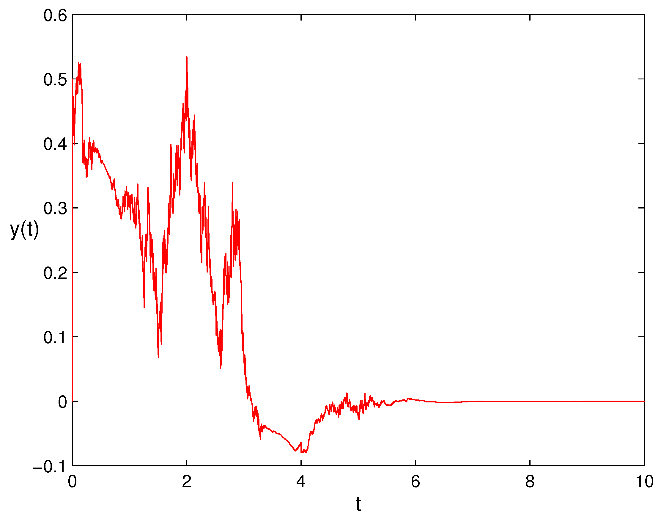
For instance, consider the following linear stochastic delay differential systems with logic impulses:

$$\left\{\begin{array}{cc}\dot{y}\left(t\right)=(-2y\left(t\right)+sinty(t-|sint|)dt+costy(t-|cost|)dw\left(t\right),\hfill & t\ge t_0,t\ne t_k,\hfill \\ \Delta y\left(t_k\right)={\left(y\left(t_k\right)\right)}^{2k+1}u\left(t_k\right)+\frac{1}{2^k}y\left(t_k\right)\overline{u\left(t_k\right)},\hfill & t=t_k,k\in N,\hfill \\ y\left(t\right)=0.5,\hfill & t\in [-1,0].\hfill \end{array}\right.$$

(19)

where $t_k=2k,k=1,2,3,\cdots$ are fixed impulsive points. Let $a\left(t\right)=-2$, $b\left(t\right)=sint$, $c\left(t\right)=cost$, $h\left(t\right)=|sint|$, $\tau \left(t\right)=|cost|$, then $a=-2$, $b=c=h=\tau =r=1$. Obviously, $a+b+{\displaystyle \frac{1}{2}}{c}^2<0$. According to the above analysis, system (19) is exponentially stable in a mean square, as shown in Figure 1.

Example 2. 

Consider the 2-dimensional nonlinear stochastic delay differential systems with logic impulses as follows:

$$\left\{\begin{array}{c}d{y}_1\left(t\right)=(-a_1{y}_1\left(t\right)-a_2{y}_1^3\left(t\right)+a_3{y}_2(t-h\left(t\right)))dt+a_4{y}_2(t-\tau \left(t\right))d{w}_1\left(t\right),\hfill \\ d{y}_2\left(t\right)=(-b_1{y}_2\left(t\right)-b_2{y}_2^3\left(t\right)+b_3{y}_1(t-h\left(t\right)))dt+b_4{y}_1(t-\tau \left(t\right))d{w}_2\left(t\right),t\ne t_k,\hfill \\ \Delta y_1\left(t_k\right)=\frac{1}{3^k}{y}_1\left(t_k\right)u_1\left(t_k\right)-\frac{1}{3^k}{y}_1\left(t_k\right)\overline{u_1\left(t_k\right)},\hfill \\ \Delta y_2\left(t_k\right)=\frac{1}{4^k}{y}_2\left(t_k\right)u_2\left(t_k\right)-\frac{1}{4^k}{y}_2\left(t_k\right)\overline{u_2\left(t_k\right)},k\in N.\hfill \end{array}\right.$$

(20)

where $a_i,b_i$, $i=1,2,3,4$ is real numbers, $0\le t_0<t_1<\dots <t_k<\dots$ are fixed impulsive points, $\underset{k\to \infty }{lim}{t}_k=\infty$, $h\left(t\right)$, $\tau \left(t\right)$ are continuous functions on $[t_0,\infty )$, $h=\underset{t\ge t_0}{sup}h\left(t\right)$, $\tau =\underset{t\ge t_0}{sup}\tau \left(t\right)$, $r=max\{h,\tau \}$.

The logical functions $u_i,{\overline{u}}_i:{\{{\delta }_2^1,{\delta }_2^2\}}^2\to \{0,1\}$ are as follows:

$$u_1\left(t\right)=p_1\left(y_1\left(t\right)\right)\overline{\vee }{p}_2\left(y_2\left(t\right)\right),\overline{u_1\left(t\right)}=\neg u_1\left(t\right)=p_1\left(y_1\left(t\right)\right)\leftrightarrow p_2\left(y_2\left(t\right)\right);$$

$$u_2\left(t\right)=p_1\left(y_1\left(t\right)\right)\wedge p_2\left(y_2\left(t\right)\right),\overline{u_2\left(t\right)}=\neg u_2\left(t\right)=p_1\left(y_1\left(t\right)\right)\uparrow p_2\left(y_2\left(t\right)\right).$$

The piecewise function $p_i:R\to \{0,1\}$ has the following form:

$$p_1\left(s\right)=\left\{\begin{array}{c}{\delta }_2^2\sim 0,|s-0.1|\ge 0.05,\hfill \\ {\delta }_2^1\sim 1,|s-0.1|<0.05.\hfill \end{array}\right.$$

$$p_2\left(s\right)=\left\{\begin{array}{c}{\delta }_2^2\sim 0,|s-0.05|\ge 0.15,\hfill \\ {\delta }_2^1\sim 1,|s-0.05|<0.15.\hfill \end{array}\right.$$

that is

$$p_1\left(s\right)=\left\{\begin{array}{c}{\delta }_2^2\sim 0,otherwise,\hfill \\ {\delta }_2^1\sim 1,0.05<s<0.15.\hfill \end{array}\right.$$

$$p_2\left(s\right)=\left\{\begin{array}{c}{\delta }_2^2\sim 0,otherwise,\hfill \\ {\delta }_2^1\sim 1,-0.1<s<0.2.\hfill \end{array}\right.$$

here, $q_1\left(s\right)=s-0.1,q_2\left(s\right)=s-0.05$, $0.05$ and $0.15$ are the threshold values.

Let $p\left(y\left(t_k\right)\right)={⋉}_{i=1}^2{p}_i\left(y_i\left(t_k\right)\right)$, ${\varphi }_k\left(y_1\left(t_k\right)\right)=[{\displaystyle \frac{1}{3^k}},-{\displaystyle \frac{1}{3^k}}]y_1\left(t_k\right)$, ${\varphi }_k\left(y_2\left(t_k\right)\right)=$$[{\displaystyle \frac{1}{4^k}},-{\displaystyle \frac{1}{4^k}}]y_2\left(t_k\right)$, $M_1={\delta }_2(2,1,1,2)$, $M_2={\delta }_2(1,2,2,2)$. By applying the semi-tensor product method, we have $\Delta y_i\left(t_k\right)={\varphi }_k\left(y_i\left(t_k\right)\right)M_{i}p\left(y\left(t_k\right)\right),i=1,2.$

Furthermore, for $t\ge 0$,

$$e^{-\frac{1}{2}}\le \prod _{t_0\le t_k<t}\frac{1}{1+\frac{1}{3^k}}\le {\alpha }_1\left(t\right)\le \prod _{t_0\le t_k<t}\frac{1}{1-\frac{1}{3^k}}\le e^{\frac{1}{2}},$$

$$e^{-\frac{1}{3}}\le \prod _{t_0\le t_k<t}\frac{1}{1+\frac{1}{4^k}}\le {\alpha }_2\left(t\right)\le \prod _{t_0\le t_k<t}\frac{1}{1-\frac{1}{4^k}}\le e^{\frac{1}{3}}.$$

Obviously, ${\alpha }_1^{-1}\left(t\right)$ and ${\alpha }_2^{-1}\left(t\right)$ are bounded. Thus, there exists a constant $M>0$ such that $\parallel {\alpha }^{-1}\left(t\right)\parallel \le M$. Let $\chi ={(e^{\frac{1}{2}},e^{\frac{1}{3}})}^T$, $\alpha \left(t\right)={({\alpha }_1\left(t\right),{\alpha }_2\left(t\right))}^T$, it is easy to see that $\alpha \left(t\right)\le \chi$ for any $t\ge 0$.

Assume that $a_2,b_2>0$. Then, for any $t\ge 0$, $x={(x_1,x_2)}^T$, $z={(z_1,z_2)}^T$,

$$\begin{array}{cc}\hfill x_1{f}_1(t,x,z)& =-a_1{x}_1^2-a_2{x}_1^4+a_3{x}_1{z}_2\hfill \\ \hfill & \le -a_1{x}_1^2+\frac{|a_3|}{2}(x_1^2+z_2^2)\hfill \\ \hfill & =(-a_1+\frac{|a_3|}{2})x_1^2+\frac{|a_3|}{2}{z}_2^2,\hfill \end{array}$$

and

$$\begin{array}{cc}\hfill x_2{f}_2(t,x,z)& =-b_1{x}_2^2-b_2{x}_2^4+b_3{x}_2{z}_1\hfill \\ \hfill & \le -b_1{x}_2^2+\frac{|b_3|}{2}(x_2^2+z_1^2)\hfill \\ \hfill & =(-b_1+\frac{|b_3|}{2})x_2^2+\frac{|b_3|}{2}{z}_1^2.\hfill \end{array}$$

Meanwhile, $g_{12}(t,x,z)=0$, $g_{21}(t,x,z)=0$, $g_{11}(t,x,z)=a_4{z}_2$, $g_{22}(t,x,z)=b_4{z}_1$. Thus,

$$g_{11}^2(t,x,z)=a_4^2{z}_2^2,g_{12}^2(t,x,z)=0,g_{21}^2(t,x,z)=0,g_{22}^2(t,x,z)=b_4^2{z}_1^2.$$

The constant matrices are taken as follows:

$$A=\left[\begin{array}{cc}-a_1+\frac{1}{2}\left|a_3\right|& 0\\ 0& -b_1+\frac{1}{2}\left|b_3\right|\end{array}\right],B=\left[\begin{array}{cc}0& \frac{1}{2}\left|a_3\right|\\ \frac{1}{2}\left|b_3\right|& 0\end{array}\right],$$

$$A_1=A_2=0,B_1=\left[\begin{array}{cc}0& a_4^2\\ 0& 0\end{array}\right],B_2=\left[\begin{array}{cc}0& 0\\ b_4^2& 0\end{array}\right].$$

Then, according to Theorem 1, the trivial solution of (20) is exponentially stable in the mean square if the following matrix is Hurwitz stable:

$$A+B+\frac{1}{2}{\chi }^{*}\circ (A_1+A_2+B_1+B_2)=\left[\begin{array}{cc}-a_1+\frac{1}{2}\left|a_3\right|& \frac{1}{2}\left|a_3\right|+\frac{1}{2}{a}_4^2{e}^{\frac{1}{2}}\\ \frac{1}{2}\left|b_3\right|+\frac{1}{2}{b}_4^2{e}^{\frac{1}{3}}& -b_1+\frac{1}{2}\left|b_3\right|\end{array}\right]:=\Xi$$

where ${\chi }^{*}:=(\chi ,\chi )\in R^{2\times 2}$.

We can set the conditions of the Hurwitz-stable matrix according to Lemma 2, two examples are given below.

Case I. Let vector $p={(1,1)}^T$, then $\Xi p\ll 0$ holds if and only if

$$\left\{\begin{array}{c}-a_1+\frac{1}{2}|a_3|+\frac{1}{2}\left|a_3\right|+\frac{1}{2}{a}_4^2{e}^{\frac{1}{2}}<0,\hfill \\ \frac{1}{2}|b_3|+\frac{1}{2}{b}_4^2{e}^{\frac{1}{3}}-b_1+\frac{1}{2}\left|b_3\right|<0.\hfill \end{array}\right.$$

To solve the above inequalities, when the coefficients satisfy the following conditions:

$$a_2>0,b_2>0,a_1>|a_3|+\frac{1}{2}{a}_4^2{e}^{\frac{1}{2}},b_1>\left|b_3\right|+\frac{1}{2}{b}_4^2{e}^{\frac{1}{3}},(\ast )$$

the trivial solution of (20) is exponentially stable in the mean square.

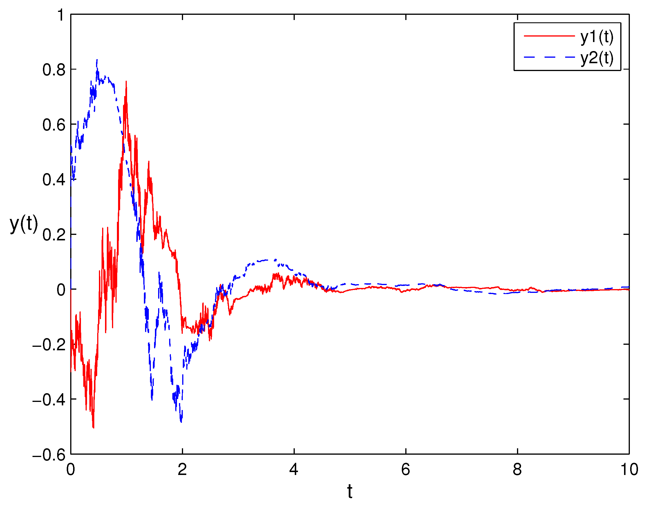
For instance, consider the following nonlinear stochastic delay differential systems with logic impulses:

$$\left\{\begin{array}{c}d{y}_1\left(t\right)=(-1.9y_1\left(t\right)-0.9y_1^3\left(t\right)+y_2(t-\frac{1}{4}|sint|\left)\right)dt-y_2(t-\frac{1}{2}|cost|)d{w}_1\left(t\right),\hfill \\ d{y}_2\left(t\right)=(-1.8y_2\left(t\right)-0.8y_2^3\left(t\right)-y_1(t-\frac{1}{4}|sint|\left)\right)dt+y_1(t-\frac{1}{2}|cost|)d{w}_2\left(t\right),t\ne t_k,\hfill \\ \Delta y_1\left(t_k\right)=\frac{1}{3^k}{y}_1\left(t_k\right)u_1\left(t_k\right)-\frac{1}{3^k}{y}_1\left(t_k\right)\overline{u_1\left(t_k\right)},\hfill \\ \Delta y_2\left(t_k\right)=\frac{1}{4^k}{y}_2\left(t_k\right)u_2\left(t_k\right)-\frac{1}{4^k}{y}_2\left(t_k\right)\overline{u_2\left(t_k\right)},k\in N.\hfill \end{array}\right.$$

(21)

where $t_k=2k,k=1,2,3,\cdots$ are fixed impulsive points. The initial condition is: $y_1\left(t\right)=-0.3,$$y_2\left(t\right)=0.5,t\in [-\frac{1}{2},0]$. Let $a_1=1.9,a_2=0.9,a_3=1,a_4=-1$, $b_1=1.8,b_2=0.8,b_3=-1,b_4=1$ which are satisfying inequality condition $(\ast )$, then, system (21) is exponentially stable in the mean square, showed in Figure 2.

Case II. Let vector $p={(e^{-\frac{1}{3}},e^{-\frac{1}{2}})}^T$, then $\Xi p\ll 0$ holds if and only if

$$\left\{\begin{array}{c}-e^{-\frac{1}{3}}{a}_1+\frac{1}{2}{e}^{-\frac{1}{3}}|a_3|+\frac{1}{2}{e}^{-\frac{1}{2}}\left|a_3\right|+\frac{1}{2}{a}_4^2<0,\hfill \\ \frac{1}{2}{e}^{-\frac{1}{3}}|b_3|+\frac{1}{2}{b}_4^2-e^{-\frac{1}{2}}{b}_1+\frac{1}{2}{e}^{-\frac{1}{2}}\left|b_3\right|<0.\hfill \end{array}\right.$$

To solve the above inequalities, when the coefficients satisfy the following conditions:

$$a_2>0,b_2>0,a_1>\frac{1}{2}(1+e^{-\frac{1}{6}})|a_3|+\frac{1}{2}{e}^{\frac{1}{3}}{a}_4^2,b_1>\frac{1}{2}(1+e^{\frac{1}{6}})\left|b_3\right|+\frac{1}{2}{e}^{\frac{1}{2}}{b}_4^2,(\ast \ast )$$

the trivial solution of (20) is exponentially stable in the mean square.

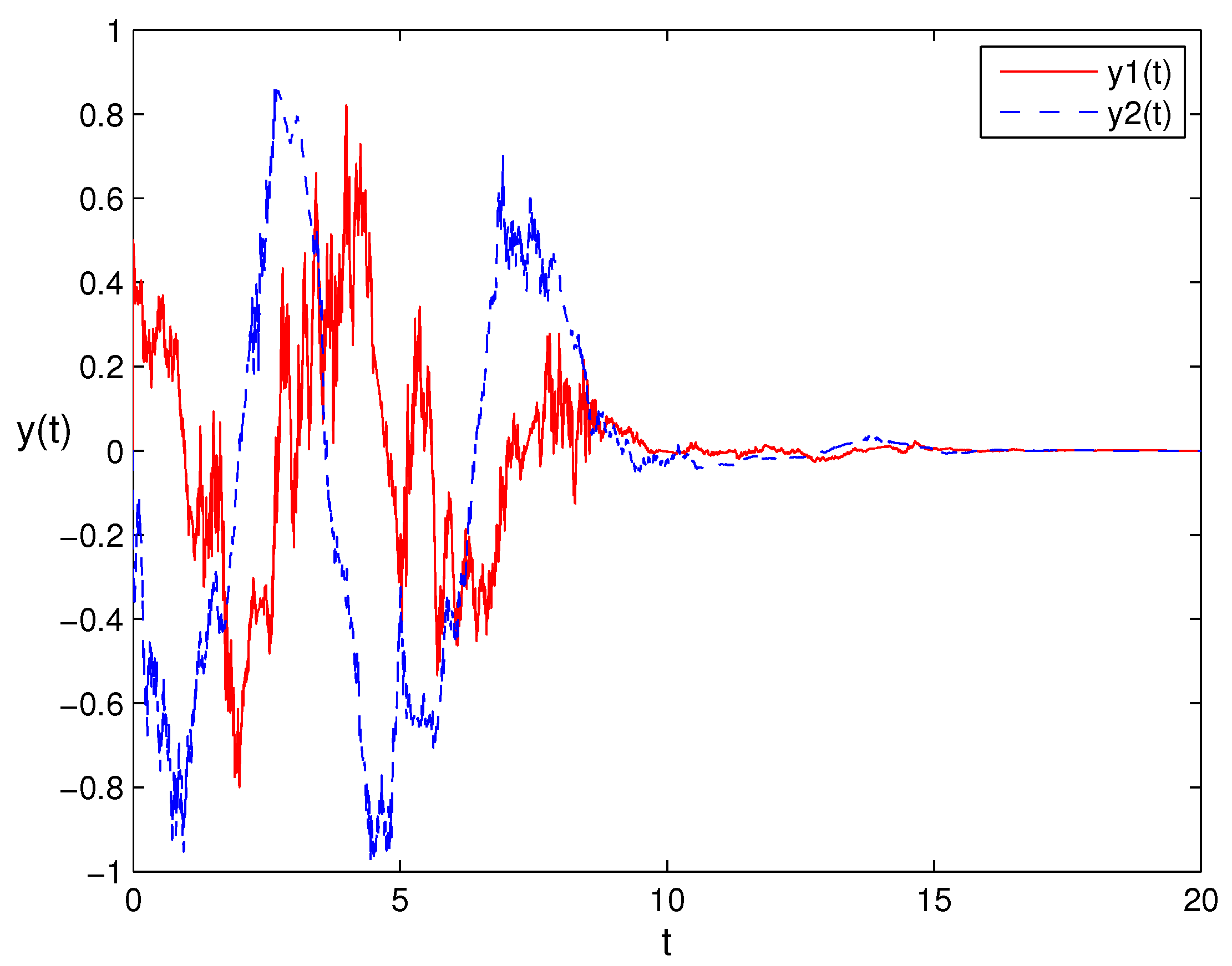
For instance, consider the following nonlinear stochastic delay differential systems with logic impulses:

$$\left\{\begin{array}{c}d{y}_1\left(t\right)=(-1.7y_1\left(t\right)-0.7y_1^3\left(t\right)+y_2(t-\frac{1}{2}|sint|\left)\right)dt-y_2(t-|cost\left|\right)d{w}_1\left(t\right),\hfill \\ d{y}_2\left(t\right)=(-2y_2\left(t\right)-y_2^3\left(t\right)-y_1(t-\frac{1}{2}|sint|\left)\right)dt+y_1(t-|cost\left|\right)d{w}_2\left(t\right),t\ne t_k,\hfill \\ \Delta y_1\left(t_k\right)=\frac{1}{3^k}{y}_1\left(t_k\right)u_1\left(t_k\right)-\frac{1}{3^k}{y}_1\left(t_k\right)\overline{u_1\left(t_k\right)},\hfill \\ \Delta y_2\left(t_k\right)=\frac{1}{4^k}{y}_2\left(t_k\right)u_2\left(t_k\right)-\frac{1}{4^k}{y}_2\left(t_k\right)\overline{u_2\left(t_k\right)},k\in N.\hfill \end{array}\right.$$

(22)

where $t_k=4k,k=1,2,3,\cdots$ are fixed impulsive points. The initial condition is: $y_1\left(t\right)=0.5,$$y_2\left(t\right)=-0.3,t\in [-1,0]$. Clearly, $a_1=1.7,a_2=0.7,a_3=1,a_4=-1$, $b_1=2,$$b_2=1,b_3=-1,b_4=1$, which satisfy inequality condition $(\ast \ast )$, then, system (22) is exponentially stable in the mean square, as shown in Figure 3.

6. Discussion

In this paper, the mean square exponential stability of nonlinear stochastic delay differential systems with logic impulses has been investigated. First of all, the nonlinear stochastic delay differential system with logic impulses is constructed, and the impulsive effects including logic function are transformed into algebraic expressions by using the semi-tensor product method. Then, some stability criteria, which do not require the construction of the Lyapunov functions, are provided for the nonlinear stochastic delay differential systems with logic impulses by establishing the equivalence relation between the solutions of the nonlinear stochastic delay differential systems with logic impulses and a corresponding nonlinear stochastic delay differential system without impulses. At last, two kinds of stochastic delay differential systems with uncertain parameters and logic impulses are discussed. The coefficient conditions guaranteeing the mean square exponential stability of these two systems are obtained by using our stability criteria.