An Inventory Model with Advertisement- and Customer-Relationship-Management-Sensitive Demand for a Product’s Life Cycle

Abstract

Advertisements play an important role in communicating with target customers. A higher advertisement frequency increases costs but may increase the chances of acquiring new customers. Moreover, faced with a wide-ranging array of products that might fit specific needs, customers usually buy according to expectations about value and satisfaction. When customers are satisfied with a purchasing experience, they are more likely to buy again and share their experiences with others. Hence, companies are concerned about increasing customer value and service satisfaction to develop and manage customer relationships. This maintains a company’s competitive edge and can improve its market share. In this article, we incorporate the frequency of advertisements and the cost of customer relationship management (CRM) into the demand function under a product life cycle (PLC). Customers can return products in the appreciation period offered by a retailer. A profit-maximizing model is developed to analyze the joint marketing and ordering policy of each stage of a product’s life cycle with a product return guarantee. We construct an algorithm to identify the optimal decisions. Finally, numerical examples are presented to illustrate the proposed model, and managerial insights are obtained from a sensitivity analysis, followed by conclusions and future research.

1. Introduction

After a new product is launched, its sales grow, mature, and decline throughout the product’s life cycle. Although it is unrealistic to expect a product to sell forever, a company may nevertheless seek to earn an adequate level of profitability to afford the effort and risk. Product sales over a typical product life cycle comprise five distinct stages, as shown in Figure 1. As a result, an appropriate inventory policy at each stage of a product’s life cycle should be developed according to the level of product sales.

Over recent decades, researchers have discussed different patterns of demand matching at different stages of the product life cycle. The assumption of a constant demand in the traditional economic order quantity (EOQ) model only aligns with the maturity stage of a product’s life cycle. In order to reflect the reality, the earlier research has generally assumed that demand rate is a linear or exponential function, increasing during the introduction and growth stages and decreasing during the decline stage. Donaldson [1] established a classical inventory model with a linear trend in demand and no shortages over a finite time-horizon. Henery [2] further expanded the demand rate from the work of Donaldson [1] to develop general log-concave demand functions. Teng and Yang [3] developed a replenishment policy where the demand function fluctuated with time, and it included increasing, decreasing, and log-concave demand patterns. On the other hand, demand for a product over its life cycle may increase initially and then remain constant for a certain period before finally declining. Hill [4] and Ahmed et al. [5] proposed a ramp-type demand rate using the EOQ model in which the demand increased with time up to a certain level and then became constant over the rest of the period. To depict a product demand pattern more reasonably through a life cycle, Cheng and Wang [6] extended the deteriorating inventory model to allow for a trapezoidal-type demand rate, which included the stages from market introduction to decline over a product’s life cycle. Skouri and Konstantaras [7] and Lin et al. [8] explored a time-varying deteriorating inventory model with a trapezoidal-type demand rate by introducing shortages. Wu et al. [9] discussed pricing and inventory decisions in an inventory model by considering that product freshness was linked to expiration date, and the demand rate was a trapezoidal, multivariate function of price and time. Inventory control requires maintaining an adequate stock level of a product to meet customer demand and, in turn, achieving the possible lowest cost or the highest possible profit. The analysis of the inventory models that allow for a constant rate of demand to vary over time has broadened the field of inventory management in practice.

In order to keep and sustain a competitive advantage, a retailer offers an appreciation period in which customers can request a return or exchange when they are dissatisfied with a product. According to online shopping surveys conducted by Pinkerton [10] and Trager [11], over 70% of the respondents evaluated the return conditions of a store before they made purchase decisions. Petersen and Kumar [12] demonstrated that a lenient return policy builds customer trust and convenience in shopping experiences, and hence, this leads to future repeat purchases. Yalabik et al. [13] introduced an optimal returns system that coordinated decisions in marketing and logistics. They identified that a refund policy decreases perceived risk and provides a protection mechanism for customers to go ahead with a purchase. Chen and Bell [14] designed a dual-channel structure with different returns policies—full-refund and no-returns—to examine the impact of customer returns on a firm’s pricing and inventory decisions. They illustrated how a firm could enhance profitability using their dual-channel structure. Akçay et al. [15] considered a retailer who adopted a money-back guarantee policy and resold returned products by discounting them as open-box items. They studied the retailer’s optimal pricing, order quantities, and refunded amounts, and how the retailer’s profit by the restock and resale of returned products had increased. Hu et al. [16] found that a vendor would not offer a return policy if the salvage value was zero in an inventory control problem under a consignment contract. In the research of Priyan and Uthayakumar [17], defective recoverable products were returned to a warehouse by a distributor, and the warehouse recovered them into perfect products under a recovery inventory system. Ülkü and Gürler [18] introduced a newsvendor model in which customers could decide to keep a product or exercise an abused or normal return after using it. Li et al. [19] studied a two-tier supply chain problem with a manufacturer and a retailer where the pricing and ordering decisions were made along with the retailer’s product returns policy over two time periods. Assuming that customers could return a product at any stage of the replenishment cycle, Kumari and De [20] analyzed the impact of both returns and trade credit policies on the EOQ model, considering resalable returns for deteriorating items. Unlike the study of Kumari and De [20], Cheng and Ouyang [21] assumed that a retailer only offered a no-reason return period (an appreciation period) to its customers. They investigated the optimal pricing and ordering policies in an advanced sales system where a retailer could receive a supplier’s trade credit. Later, considering an advance sales system within a no-reason return period and two-phase advance sales, Cheng et al. [22] established a deteriorating EOQ model to determine a retailer’s optimal sales periods and selling prices.

Kotler and Armstrong [23] proposed that achieving marketing goals depends on not only attracting customers but also on maintaining and growing customer numbers. Delivering the desired satisfactions is a key influence on future buying behavior. To reach their target markets, companies rely heavily on advertising, which serves to inform, persuade, and remind consumers about their products or services. Through mass media channels, advertising effectively communicates a company’s or brand’s value proposition to potential customers. In addition, customer relationship management is an important business strategy for businesses looking to build strong, lasting relationships with their customers. When customers feel that a business understands and cares about their needs, they are more likely to stay loyal to that business. By doing so, advertising and customer relationship management help create a positive perception of a company or brand, which, in turn, leads to an increase in customer referrals through word of mouth. Urban [24] developed a finite replenishment inventory model by incorporating the influence of price variations and advertising expenditures on demand. Lee and Kim [25] examined the effects of integrated lot sizing and marketing expenditure decisions through an extended pricing-EOQ model context. Sadjadi et al. [26] considered an inventory model by assuming that production rate is a linear function of demand. Their model formulation determined a product’s selling price, production lot size, and marketing expenditure. Wang et al. [27] established a newsvendor-type coordination model consisting of a manufacturer and a buyer by considering the combined effect of advertising expenditure and selling price on demand. Yadav et al. [28] investigated an inventory problem with backorders by assuming demand to depend on the frequency of advertisements in a fuzzy environment. Rabbani et al. [29] proposed a joint pricing and inventory control problem for non-instantaneous deteriorating items in which the demand rate was a function of both the selling price and the frequency of advertisements. Manna et al. [30] extended an imperfect production inventory model by accounting for an advertisement-dependent demand rate, which was assumed to be an increasing function of time at a decreasing rate. Shaikh et al. [31] considered the effects of selling price and frequency of advertisements on demand in a deteriorating inventory model which allowed for a permissible delay in payments and a time-proportional backlogging rate. Because advertisements can spread out the popularity of a product for all categories of customers, Khan et al. [32] expanded the deteriorating inventory model by considering an advertisement policy with an advanced payment policy. They assumed that the demand for a product with a maximum lifetime depended on the frequency of advertisements, which was confined to a positive integer, and the selling price. San-José et al. [33] obtained an optimal advertising policy adopting a power form of demand dependent on the selling price, time, and frequency of advertisements in a lot-size inventory problem. Mandal and Pal [34] dealt with an EPQ model under an imperfect production system where demand was dependent on selling price and advertisements. In a two-level supply chain model with unreliable production process, Giri and Dash [35] derived an optimal batch shipment policy under price, advertisement frequency, and green-sensitive demand.

In reality, customer returns are the major category of returns in the supply chain. Retailers should use effective CRM to communicate their return policies across multiple channels. As a result, customer returns put pressure on a firm’s costs arising from various activities, including CRMs and returns. In addition, advertising and CRMs are widely used by firms to communicate with customers in a competitive environment. Motivated by previous studies and investigations, this study aimed to address existing research gaps by developing an inventory model that links a firm’s profit, incorporating the effects of advertising, with a CRM and an appreciation period. In the literature, advertising models with return policies have been extensively studied. However, there is a lack of research investigating the effects of advertising, CRMs, and appreciation periods within a product’s life cycle. This study endeavored to address this gap by making contributions to three streams of literature: (1) an inventory model with a return policy, (2) an inventory model with advertisement-sensitive demand, and (3) an inventory model with time-dependent demand. In this paper, we discuss the inventory issues, including the product life cycle, and we incorporate the frequency of advertisements and the cost of customer relationship management into the demand function. In our model, a retailer offers an appreciation period in which customers can make a request to return products when they are dissatisfied with the products. A comparison of the present paper with the relevant literature is provided in

Table 1. A comparison among the present model and related previous research.

			Demand Rate
Authors	Model Type	Return Policy	Advertisement-Dependent	CRM Cost-Dependent	Appreciation Period-Dependent	Time-Dependent
Ahmed et al. [5]	EOQ	No	No	No	No	Ramp type
Ahmed et al. [8]	EOQ	No	No	No	No	Trapezoidal type
Wu et al. [9]	EOQ	No	No	No	No	Trapezoidal type
Li et al. [19]	A two-tier supply chain	Yes	No	No	No	No
Kumari and De [20]	EOQ	Yes	No	No	No	Exponential increasing/decreasing
Cheng et al. [22]	EOQ	Yes	No	No	No	No
Khan et al. [32]	EOQ	No	DV	No	No	No
San-Jose et al. [33]	EOQ	No	DV	No	No	Power pattern
Mandal and Pal [34]	EPQ	No	DV	No	No	No
Giri and Dash [35]	A two-level supply chain	No	DV	No	No	No
Present model	Single period	Yes	DV	DV	DV	Mixture

Note: “DV” represents “Decision variable”.

to help the readers understand the contributions of our model. We established a proper model and then provided an easy and useful algorithm to obtain the optimal ordering and advertisement policies for a retailer to achieve its maximum total profit. Finally, numerical examples are given to illustrate the solution procedure, and a sensitivity analysis is performed to investigate the effects of changes in some main parameter values on the optimal solution. This paper is organized as follows: Section 1 provides a comprehensive review of the related literature. Section 2 describes the problem and provides the developed model in detail. Section 3 presents the theoretical results and provides an algorithm for searching the optimal solutions. Section 4 illustrates numerical examples and a sensitivity analysis to provide further insights. Finally, Section 5 presents the conclusions and directions for future research.

2. Problem Description and Model Formulation

2.1. Notation and Assumptions

The mathematical model in this paper was developed using the below notation and assumptions.

Notation:
p	selling price/unit
c	purchase cost/unit, where $c<p$
s	ordering cost/order
$c_a$	cost of each advertisement
h	holding cost/unit/unit time
N	appreciation period
$\rho$	return rate during the appreciation period, where $0\le \rho <1$
${\left(.\right)}_i$	parameter or decision variable at the stage in the life cycle of the product, where $i=1, 2, 3, 4$ corresponds to the four stages of introduction, growth, maturity, and decline
$M_i$	customer relationship management cost of stage i, $i=1, 2, 3, 4$/unit of time (we do not consider customer relationship management costs at the introduction stage, that is, $M_1=0$)
$t_i$	time length of stage i, $i=1, 2, 3, 4$
T	length of a product’s life cycle, $T=t_1+t_2+t_3+t_4$
$A_i$	frequency of advertisements of stage i, $i=1,2,3$ (we do not consider the frequency of advertisements at the decline stage, that is, $A_4=0$)
$Q_i$	order quantity in stage i, $i=1, 2, 3, 4$
$Z_i\left(A_i, t_i, M_i\right)$	retailer total profit for stage i, $i=1, 2, 3, 4$, where $M_1=0$ and $A_4=0$
Z	retailer total profit for a product’s life cycle, $Z=Z_1+Z_2+Z_3+Z_4$
$t_i^{*}$	optimal length of stage i for a product’s life cycle, $i=1, 2, 3, 4$
$T^{*}$	optimal product life cycle
$M_i^{*}$	optimal customer relationship management cost per unit of time for stage i, $i=2, 3, 4$
$A_i^{*}$	optimal frequency of advertisements for stage i, $i=1, 2, 3$
$Q_i^{*}$	optimal order quantity of stage i, $i=1, 2, 3, 4$
$Z_i^{*}$	retailer optimal total profit for stage i, $Z_i^{*}=Z_i\left(A_i^{*}, t_i^{*},M_i^{*}\right)$, $i=1, 2, 3, 4$, where $M_1^{*}=0$ and $A_4^{*}=0$
$Z^{*}$	retailer optimal total profit for a product’s life cycle, $Z^{*}=Z_1^{*}+Z_2^{*}+Z_3^{*}+Z_4^{*}$

• Assumptions:

  (1)

  The demand rate is a function of time, appreciation period, customer relationship management cost, and frequency of advertisements (see, for example, Cheng and Wang [6], and Rabbani et al. [29]). The demand rates of different stages are as follows:

  (1.1)

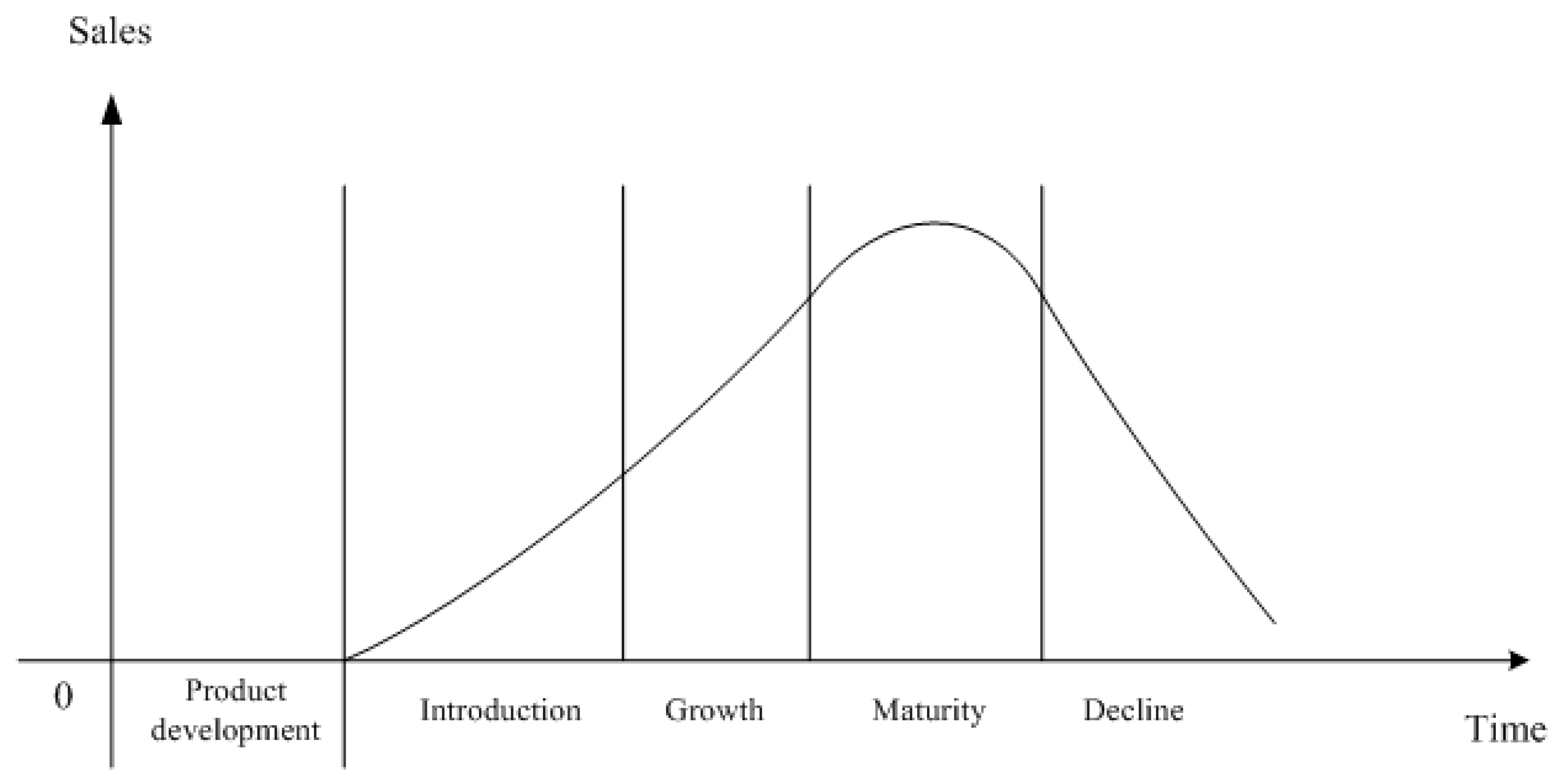
  Product introduction stage: The marketing objective is to create product awareness and trials. The demand rate is a function of time, appreciation period, and frequency of advertisements, that is, $D_1\left(A_1,t\right)=\left(a_1+b_{1}N t\right){\left(1+A_1\right)}^{\lambda }$, where $a_1>0$, $b_1>0$, $0< \lambda <1$, and $0<t<t_1$.

  (1.2)

  Product growth stage: The marketing objective is to maximize market share. The demand rate is a function of time, appreciation period, customer relationship management cost, and frequency of advertisements, that is, $D_2\left(A_2,t,M_2 \right)=\left(a_2+N^{b_2\left(t+M_2\right)}\right){\left(1+A_2\right)}^{\lambda }$, where $a_2>0$, $b_2>0$, $0<\lambda <1$, and $0<t<t_2$.

  (1.3)

  Product maturity stage: The marketing objective is to maximize profit while defending market share. The demand rate is a function of the appreciation period, customer relationship management cost, and frequency of advertisements, that is, $D_3\left(A_3,M_3\right)=a_3{\left(N+M_3\right)}^{b_3}{\left(1+A_3\right)}^{\lambda }$, where $a_3>0$, $b_3>0$, $0<\lambda <1$, and $0<t<t_3$.

  (1.4)

  Product decline stage: The marketing objective is to reduce expenditures and extract value from the brand. Sales may plunge to zero, or they may drop to a low level, where they will continue for many years. The demand rate is a function of time and customer relationship management cost. that is, $D_4\left(t,M_4 \right)=a_4\left(N+M_4\right){\left(\frac{1}{b_4}\right)}^t$, where $a_4>0$, $b_4>1$, and $0<t<t_{ 4}$.

  (2)

  During the appreciation period N, customers can make a request to return products if they are dissatisfied with them. In such cases, the retailer will refund the money and the returned products will be discarded.

2.2. Mathematical Formulation

In this paper, we discuss the optimal ordering and marketing policies for four distinct stages of the product life cycle and the optimal ordering and marketing policies for a product’s life cycle. The four distinct stages of the product life cycle are as follows: (1) introduction, (2) growth, (3) maturity, and (4) decline. We have developed retailer inventory models for these four distinct stages of the product life cycle, as follows:

Stage 1.

Introduction

The demand rate is a function of time, appreciation period, and frequency of advertisements, that is, $D_1\left(A_1,t\right)=\left(a_1+b_{1}N t\right){\left(1+A_1\right)}^{\lambda }$, where $a_1>0$, $b_1>0$, $0<\lambda <1$, and $0<t<t_1$. The order quantity in this stage is:

$$Q_1={{\displaystyle \int }}_0^{t_1}{D}_1\left(A_1,t\right)\mathrm{dt}=\left(a_1{t}_1+\frac{b_{1}N}{2}{t}_1^2\right){\left(1+A_1\right)}^{\lambda }.$$

The total profit consists of the following elements:

(a)

sales revenue ($p{Q}_1$)

(b)

purchasing cost (c$Q_1$)

(c)

returned product cost ($p\rho Q_1$)

(d)

advertisement cost ($c_a{A}_1$)

(e)

ordering cost (s)

(f)

holding cost, which is calculated by:

$$h{{\displaystyle \int }}_0^{t_1}{D}_1\left(A_1,t\right)t \mathrm{dt}=h\left(\frac{a_1}{2}{t}_1^2+\frac{b_{1}N}{3}{t}_1^3\right){\left(1+A_1\right)}^{\lambda }.$$

Therefore, a retailer’s total profit for the introduction stage is:

$Z_1\left(A_1, t_1\right)=$ sales revenue − purchasing cost − cost of return products − advertisement cost − ordering cost − holding cost, which is determined by:

$$=\left(p-c-p\rho \right)\left(a_1{t}_1+\frac{b_{1}N}{2}{t}_1^2\right){\left(1+A_1\right)}^{\lambda }-c_a{A}_1-s$$

$$-h\left(\frac{a_1}{2}{t}_1^2+\frac{b_{1}N}{3}{t}_1^3\right){\left(1+A_1\right)}^{\lambda }.$$

(1)

Stage 2.

Growth

The demand rate is a function of time, appreciation period, customer relationship management cost, and frequency of advertisements, that is, $D_2\left(A_2,t,M_2 \right)=\left(a_2+N^{b_2\left(t+M_2\right)}\right){\left(1+A_2\right)}^{\lambda }$, where $a_2>0$, $b_2>0$, $0<\lambda <1$, and $0<t<t_2$. The order quantity in this stage is:

$$Q_2={{\displaystyle \int }}_0^{t_2}{D}_2\left(A_2,t,M_2\right)dt=\left(a_2{t}_2+\frac{N^{b_2\left(t_2+M_2\right)}}{b_2\ln N}-\frac{N^{b_2{M}_2}}{b_2\ln N}\right){\left(1+A_2\right)}^{\lambda }.$$

The total profit consists of the following elements:

(a)

sales revenue ($p{Q}_2$)

(b)

purchasing cost ($c{Q}_2$)

(c)

return products cost ($p\rho Q_2$)

(d)

advertisement cost ($c_a{A}_2$)

(e)

customer relationship management cost ($\left(1-\rho \right)M_2{Q}_2$)

(f)

ordering cost (s)

(g)

holding cost, which is calculated by:

$$h{{\displaystyle \int }}_0^{t_2}{D}_2\left(A_2,t,M_2\right)t dt=h\left[\frac{a_2}{2}{t}_2^2+\frac{N^{b_2\left(t_2+M_2\right)}}{b_2\ln N}{t}_2-\frac{N^{b_2\left(t_2+M_2\right)}}{b_2^2{\left(\ln N\right)}^2}+\frac{N^{b_2{M}_2}}{b_2^2{\left(\ln N\right)}^2}\right]{\left(1+A_2\right)}^{\lambda }$$

Therefore, a retailer’s total profit for the growth stage is:

$Z_2\left(A_2, t_2, M_2\right)=$ sales revenue − purchasing cost − cost of return products − advertisement cost − cost of customer relationship management − ordering cost − holding cost, which is determined by:

$$=\left[p-c-p\rho -\left(1-\rho \right)M_2\right]\left(a_2{t}_2+\frac{N^{b_2\left(t_2+M_2\right)}}{b_2\ln N}-\frac{N^{b_2{M}_2}}{b_2\ln N}\right){\left(1+A_2\right)}^{\lambda }$$

$$-c_a{A}_2-s-h\left[\frac{a_2}{2}{t}_2^2+\frac{N^{b_2\left(t_2+M_2\right)}}{b_2\ln N}{t}_2-\frac{N^{b_2\left(t_2+M_2\right)}}{b_2^2{\left(\ln N\right)}^2}+\frac{N^{b_2{M}_2}}{b_2^2{\left(\ln N\right)}^2}\right]{\left(1+A_2\right)}^{\lambda }$$

(2)

Stage 3.

Maturity

The demand rate is a function of the appreciation period, customer relationship management cost, and frequency of advertisements, that is, $D_3\left(A_3,M_3\right)=a_3{\left(N+M_3\right)}^{b_3}{\left(1+A_3\right)}^{\lambda }$, where $a_3>0$, $b_3>0$, $0<\lambda <1$, and $0<t<t_3$. The order quantity in this stage is:

$$Q_3={{\displaystyle \int }}_0^{t_3}{D}_3\left(A_3,M_3\right)dt=a_3{\left(N+M_3\right)}^{b_3}{\left(1+A_3\right)}^{\lambda }{t}_3.$$

The total profit consists of the following elements:

(a)

sales revenue ($p{Q}_3$)

(b)

purchasing cost ($c{Q}_3$)

(c)

return products cost ($p\rho Q_3$)

(d)

advertisement cost ($c_a{A}_3$)

(e)

customer relationship management cost ($\left(1-\rho \right)M_3{Q}_3$)

(f)

ordering cost (s)

(g)

holding cost, which is calculated by:

$$h{{\displaystyle \int }}_0^{t_3}{D}_3\left(A_3,M_3\right)tdt=\frac{h}{2}{a}_3{\left(N+M_3\right)}^{b_3}{\left(1+A_3\right)}^{\lambda }{t}_3^2.$$

Therefore, a retailer’s total profit for the maturity stage is:

$Z_3\left(A_3, t_3, M_3\right)=$ sales revenue − purchasing cost − cost of return products—advertisement cost − cost of customer relationship management—ordering cost—holding cost, which is determined by:

$$\begin{gathered} =\left[p-c-p\rho -\left(1-\rho \right)M_3\right]a_3{\left(N+M_3\right)}^{b_3}{\left(1+A_3\right)}^{\lambda }{t}_3-c_a{A}_3 \\ -s-\frac{h}{2}{a}_3{\left(N+M_3\right)}^{b_3}{\left(1+A_3\right)}^{\lambda }{t}_3^2. \end{gathered}$$

(3)

Stage 4.

Decline

The demand rate is a function of time and customer relationship management cost, that is, $D_4\left(t,M_4 \right)=a_4\left(N+M_4\right){\left(\frac{1}{b_4}\right)}^t$, where $a_4>0$, $b_4>1$, and $0<t<t_{ 4}$. The order quantity in this stage is calculated by:

$$Q_4={{\displaystyle \int }}_0^{t_4}{D}_4\left(t,M_4 \right)dt=\frac{a_4\left(N+M_4\right)}{\ln b_4}\left(1-b_4^{-t_4}\right).$$

The total profit consists of the following elements:

(a)

sales revenue ($p{Q}_4$)

(b)

purchasing cost ($c{Q}_4$)

(c)

return products cost ($p\rho Q_4$)

(d)

customer relationship management cost ($\left(1-\rho \right)M_4{Q}_4$)

(e)

ordering cost (s)

(f)

holding cost, which is calculated by:

$$h{{\displaystyle \int }}_0^{t_4}{D}_4\left(t,M_4 \right)t dt=h{a}_4\left(N+M_4\right)\left[\frac{1}{{\left(\ln b_4\right)}^2}-\frac{t_4{b}_4^{-t_4}}{\ln b_4}-\frac{b_4^{-t_4}}{{\left(\ln b_4\right)}^2}\right].$$

Therefore, a retailer’s total profit for the decline stage is:

$Z_4\left(t_4, M_4\right)=$ sales revenue − purchasing cost − cost of return products—cost of customer relationship management − ordering cost − holding cost, which is determined by:

$$\begin{gathered} =\left[p-c-p\rho -\left(1-\rho \right)M_4\right]\frac{a_4\left(N+M_4\right)}{\ln b_4}\left(1-b_4^{-t_4}\right) \\ -s-h{a}_4\left(N+M_4\right)\left[\frac{1}{{\left(\ln b_4\right)}^2}-\frac{t_4{b}_4^{-t_4}}{\ln b_4}-\frac{b_4^{-t_4}}{{\left(\ln b_4\right)}^2}\right]. \end{gathered}$$

(4)

Furthermore, a retailer’s total profit for a product’s life cycle is:

$$\begin{gathered} Z\left(A_1, A_2,A_3,t_1, t_2, t_3, t_4, M_2,M_3,M_4\right)={\mathrm{Z}}_1\left(A_1,t_1\right)+Z_2\left(A_2, t_2, M_2\right) \\ +Z_3\left(A_3, t_3, M_3\right)+Z_4\left(t_4, M_4\right). \end{gathered}$$

(5)

3. Theoretical Results

In this section, the solution procedure is presented and an algorithm is established to determine the optimal solution to the aforementioned cases. The goal was to maximize retailer total profit. First, we found the optimal solution that could maximize the retailer total profit for the four distinct stages of the product life cycle. We, then proceeded to use the software program Mathematica 13.0 to obtain the optimal solution, $A_1^{*}, A_2^{*}, A_3^{*}, t_1^{*}, t_2^{*}, t_3^{*}, t_4^{*}, M_2^{*}, M_3^{*},M_4^{*}$, and the maximum retailer total profit for a product’s life cycle, $Z^{*}\left(A_1^{*}, A_2^{*}, A_3^{*}, t_1^{*}, t_2^{*}, t_3^{*}, t_4^{*}, M_2^{*}, M_3^{*},M_4^{*}\right)$. Then, for fixed $A_i,i=1, 2, 3,$we obtained the optimal solution that could maximize retailer total profit for the four distinct stages of the product life cycle, as follows:

Stage 1.

Introduction

To maximize the total profit, for fixed $A_1=A_1^{*}$, taking the first-order and second-order derivatives of $Z_1\left(t_1|A_1\right)$ in (1) with respect to $t_1$, we obtain

$$\frac{\partial Z_1}{\partial t_1}=\left(p-c-p\rho -h{t}_1\right)\left(a_1+b_{1}N{t}_1\right){\left(1+A_1\right)}^{\lambda },$$

(6)

and

$$\frac{{\partial }^2{Z}_1}{\partial t_1^2}=\left[\left(p-c-p\rho \right)b_{1}N-h\left(a_1+2b_{1}N{t}_1\right)\right]{\left(1+A_1\right)}^{\lambda }.$$

(7)

If $\frac{{\partial }^2{Z}_1}{\partial t_1^2}<0$, then $Z_1\left(t_1|A_1\right)$ is a concave function of $t_1$ and $Z_1\left(t_1|A_1\right)$ has its maximum value at

$$t_1=\frac{p-c-p\rho }{h}.$$

(8)

Stage 2.

Growth

To maximize the total profit, for fixed $A_2=A_2^{*}$, taking the first-order derivative of $Z_2\left(t_2,M_2|A_2\right)$ in (2) with respect to $t_2$ and $M_2$, respectively, we obtain

$$\frac{\partial Z_2}{\partial t_2}=\left[p-c-p\rho -M_2\left(1-\rho \right)-h{t}_2\right]\left[a_2+N^{b_2\left(t_2+M_2\right)}\right]{\left(1+A_2\right)}^{\lambda }$$

(9)

and

$$\begin{gathered} \frac{\partial Z_2}{\partial M_2}=+\left[p-c-p\rho -M_2\left(1-\rho \right)\right]N^{b_2{M}_2}\left(N^{b_2{t}_2}-1\right){\left(1+A_2\right)}^{\lambda } \\ -h\left[t_2{N}^{b_2\left(t_2+M_2\right)}-\frac{N^{b_2\left(t_2+M_2\right)}}{b_2\ln N}+\frac{N^{b_2{M}_2}}{b_2\ln N}\right]{\left(1+A_2\right)}^{\lambda } \\ -\left(1-\rho \right)\left[a_2{t}_2+\frac{N^{b_2\left(t_2+M_2\right)}-N^{b_2{M}_2}}{b_2\ln N}\right]{\left(1+A_2\right)}^{\lambda }. \end{gathered}$$

(10)

The optimal solution of $\left(t_2,M_2\right)$ must simultaneously satisfy $\frac{\partial Z_2}{\partial t_2}=0$ and $\frac{\partial Z_2}{\partial M_2}=0$. In addition,

$$\begin{gathered} \frac{{\partial }^2{Z}_2}{\partial t_2^2}=\left[p-c-p\rho -M_2\left(1-\rho \right)\right]N^{b_2\left(t_2+M_2\right)}{b}_2\ln N{\left(1+A_2\right)}^{\lambda } \\ -h\left[a_2+N^{b_2\left(t_2+M_2\right)}+t_2{N}^{b_2\left(t_2+M_2\right)}{b}_2\ln N\right]{\left(1+A_2\right)}^{\lambda }, \end{gathered}$$

(11)

$$\begin{gathered} \frac{{\partial }^2{Z}_2}{\partial M_2^2}=\left[p-c-p\rho -M_2\left(1-\rho \right)\right]b_2\ln N\left[N^{b_2\left(t_2+M_2\right)}-N^{b_2{M}_2}\right]{\left(1+A_2\right)}^{\lambda } \\ -2\left(1-\rho \right)\left[N^{b_2\left(t_2+M_2\right)}-N^{b_2{M}_2}\right]{\left(1+A_2\right)}^{\lambda } \\ -h\left[t_2{N}^{b_2\left(t_2+M_2\right)}{b}_2\ln N-N^{b_2\left(t_2+M_2\right)}+N^{b_2{M}_2}\right]{\left(1+A_2\right)}^{\lambda }, \end{gathered}$$

(12)

and

$$\begin{gathered} \frac{{\partial }^2{Z}_2}{\partial M_2\partial t_2}=\left[p-c-p\rho -M_2\left(1-\rho \right)-h{t}_2\right]N^{b_2\left(t_2+M_2\right)}{b}_2\ln N{\left(1+A_2\right)}^{\lambda } \\ -\left(1-\rho \right)\left[a_2+N^{b_2\left(t_2+M_2\right)}\right]{\left(1+A_2\right)}^{\lambda }. \end{gathered}$$

(13)

Due to the complexity of the problem, we could not find a simple result in which the Hessian matrix was a positive value. However, using Equations (11)–(13), we could check this condition by using the software Mathematica 13.0 in numerical examples.

Stage 3.

Maturity

To maximize the total profit, for fixed $A_3=A_3^{*}$, taking the first-order derivative of $Z_3\left(t_3,M_3|A_3\right)$ in (3) with respect to $t_3$ and $M_3$, respectively, we obtain

$$\frac{\partial Z_3}{\partial t_3}=\left[p-c-p\rho -M_3\left(1-\rho \right)-h{t}_3\right]a_3{\left(N+M_3\right)}^{b_3}{\left(1+A_3\right)}^{\lambda }$$

(14)

and

$$\begin{gathered} \frac{\partial Z_3}{\partial M_3}=\left[p-c-p\rho -M_3\left(1-\rho \right)\right]a_3{b}_3{\left(N+M_3\right)}^{b_3-1}{\left(1+A_3\right)}^{\lambda }{t}_3 \\ -\frac{h}{2}{a}_3{b}_3{\left(N+M_3\right)}^{b_3-1}{\left(1+A_3\right)}^{\lambda }{t}_3^2-\left(1-\rho \right)a_3{\left(N+M_3\right)}^{b_3}{\left(1+A_3\right)}^{\lambda }{t}_3. \end{gathered}$$

(15)

The optimal solution of $\left(t_3,M_3\right)$ must simultaneously satisfy $\frac{\partial Z_3}{\partial t_3}=0$ and $\frac{\partial Z_3}{\partial M_3}=0$. We obtain

$$t_3=\frac{p-c-p\rho -M_3\left(1-\rho \right)}{h}$$

(16)

and

$$M_3=\frac{\left(p-c-p\rho -\frac{h}{2}{t}_3\right)b_3-\left(1-\rho \right)N}{\left(1-\rho \right)\left(1+b_3\right)}.$$

(17)

In addition,

$$\frac{{\partial }^2{Z}_3}{\partial t_3^2}=-h{a}_3{\left(N+M_3\right)}^{b_3}{\left(1+A_3\right)}^{\lambda }<0,$$

(18)

$$\begin{gathered} \frac{{\partial }^2{Z}_3}{\partial M_3^2}=\left[p-c-p\rho -M_3\left(1-\rho \right)\right]a_3{b}_3\left(b_3-1\right){\left(N+M_3\right)}^{b_3-2}{\left(1+A_3\right)}^{\lambda }{t}_3 \\ -2\left(1-\rho \right)a_3{b}_3{\left(N+M_3\right)}^{b_3-1}{\left(1+A_3\right)}^{\lambda }{t}_3 \\ -\frac{h}{2}{a}_3{b}_3\left(b_3-1\right){\left(N+M_3\right)}^{b_3-2}{\left(1+A_3\right)}^{\lambda }{t}_3^2, \end{gathered}$$

(19)

and

$$\begin{gathered} \frac{\partial Z_3}{\partial t_3\partial M_3}=\left[p-c-p\rho -M_3\left(1-\rho \right)\right]a_3{b}_3{\left(N+M_3\right)}^{b_3-1} {\left(1+A_3\right)}^{\lambda } \\ -\left(1-\rho \right)a_3{\left(N+M_3\right)}^{b_3}{\left(1+A_3\right)}^{\lambda }-h{a}_3{b}_3{\left(N+M_3\right)}^{b_3-1}{\left(1+A_3\right)}^{\lambda }{t}_3 \\ =\left\{\left[p-c-p\rho -M_3\left(1-\rho \right)-h{t}_3\right]b_3-\left(1-\rho \right)\left(N+M_3\right)\right\} \\ \times a_3{\left(1+A_3\right)}^{\lambda }{\left(N+M_3\right)}^{b_3-1}. \end{gathered}$$

(20)

Due to the complexity of the problem, we were unable to find a simple result in which the Hessian matrix was a positive value. However, using Equations (18)–(20), we could check this condition by using the software Mathematica 13.0 in numerical examples.

Stage 4.

Decline

To maximize the total profit, taking the first-order derivative of $Z_4\left(t_4,M_4\right)$ in (4) with respect to $t_4$ and $M_4$, respectively, we obtain

$$\frac{\partial Z_4}{\partial t_4}=\left[p-c-p\rho -M_4\left(1-\rho \right)-h{t}_4\right]a_4\left(N+M_4\right)b_4^{-t_4}$$

(21)

and

$$\begin{gathered} \frac{\partial Z_4}{\partial M_4}=\left[p-c-p\rho -\left(1-\rho \right)\left(2M_4+N\right)\right]\frac{a_4}{\ln b_4}\left(1-b_4^{-t_4}\right) \\ -h{a}_4\left[\frac{1}{{\left(\ln b_4\right)}^2}-\frac{t_4{b}_4^{-t_4}}{\ln b_4}-\frac{b_4^{-t_4}}{{\left(\ln b_4\right)}^2}\right]. \end{gathered}$$

(22)

The optimal solution of $\left(t_4,M_4\right)$ must simultaneously satisfy $\frac{\partial Z_4}{\partial t_4}=0$ and $\frac{\partial Z_4}{\partial M_4}=0$. We obtain

$$t_4=\frac{p-c-p\rho -M_4\left(1-\rho \right)}{h}$$

(23)

and

$$M_4=\frac{\left(1-\rho \right)\left(p-N\right)-c}{2\left(1-\rho \right)}-\frac{h}{2\left(1-\rho \right)}\left[\frac{1}{\ln b_4}-\frac{t_4{b}_4^{-t_4}}{1-b_4^{-t_4}}\right].$$

(24)

In addition,

$$\frac{{\partial }^2{Z}_4}{\partial M_4^2}=-2\left(1-\rho \right)a_4\frac{1-b_4^{-t_4}}{\ln b_4}<0,$$

(25)

$$\frac{{\partial }^2{Z}_4}{\partial t_4^2}=-\left\{\left[p-c-p\rho -M_4\left(1-\rho \right)-h{t}_4\right]\ln b_4+h\right\}{a}_4\left(N+M_4\right)b_4^{-t_4}<0,$$

(26)

and

$$\frac{{\partial }^2{Z}_4}{\partial t_4\partial M_4}=a_4{b}_4^{-t_4}\left[p-c-p\rho -\left(1-\rho \right)\left(2M_4+N\right)-h{t}_4\right].$$

(27)

Due to the complex nature of the problem, we could not find a simple result in which the Hessian matrix was a positive value. However, using Equations (25)–(27), we could check this condition by using the software Mathematica 13.0 in numerical examples.

Algorithm 1. Solution Procedure

Step 1. Input the values of parameters Step 2. Introduction stage 2.1 Set i = 0 and $A_{1,i}=0$. 2.2 Using Equation (8), $t_{1,i}$ is obtained, and substituting $t_{1,i}$ into Equation (7), if $\frac{{\partial }^2{Z}_1}{\partial t_1^2}<0$, then, by substituting $t_{1,i}$ into Equation (1), $Z_{1,i}$ is obtained. Otherwise, $Z_{1,i}$= 0. 2.3 Let i = i +1 and $A_{1,i+1}=i+1$. Using Equation (8), $t_{1,i+1}$ is obtained, and substituting $t_{1,i+1}$ into Equation (7), if $\frac{{\partial }^2{Z}_1}{\partial t_1^2}<0$, then, by substituting $t_{1,i+1}$ into Equation (1), $Z_{1,i+1}$ is obtained. Otherwise, $Z_{1,i+1}$= 0. 2.4 If $Z_{1,i+1}>Z_{1,i}$, we can proceed to 2.3. Otherwise, $Z_{1,i}=Z_1^{*}$, $t_{1,i}=t_1^{*}$, and $A_{1,i}=A_1^{*}$. Proceed to Step 6. Step 3. Growth stage 3.1 Set i = 0 and $A_{2,i}=0$. 3.2 Using Equations (9) and (10), and by simultaneously solving $\frac{\partial Z_2}{\partial t_2}=0$ and $\frac{\partial Z_2}{\partial M_2}=0$, we obtain $t_{2,i}$ and $M_{2,i}$. Substituting $t_{2,i}$ and $M_{2,i}$ into Equations (11)–(13), if the Hessian matrix has a positive value, then, by substituting $t_{2,i}$ and $M_{2,i}$ into (2), $Z_{2,i}$ is obtained. Otherwise, $Z_{2,i}$= 0. 3.3 Let i = i +1 and $A_{2,i+1}=i+1$. Using Equations (9) and (10), and by simultaneously solving $\frac{\partial Z_2}{\partial t_2}=0$ and $\frac{\partial Z_2}{\partial M_2}=0$, we obtain $t_{2,i+1}$ and $M_{2,i+1}$. Substituting $t_{2,i+1}$ and $M_{2,i+1}$ into Equations (11)–(13), if the Hessian matrix has a positive value, then, by substituting $t_{2,i+1}$ and $M_{2,i+1}$ into (2), $Z_{2,i+1}$ is obtained. Otherwise, $Z_{2,i+1}$= 0. 3.4 If $Z_{2,i+1}>Z_{2,i}$, we can proceed to 3.3. Otherwise, $Z_{2,i}=Z_2^{*}$, $t_{2,i}=t_2^{*}$, $M_{2,i}=M_2^{*}$, and $A_{2,i}=A_2^{*}$. Proceed to Step 6. Step 4. Maturity stage 4.1 Set i = 0 and $A_{3,i}=0$. 4.2 Using Equations (16) and (17), we obtain $t_{3,i}$ and $M_{3,i}$. Substituting $t_{3,i}$ and $M_{3,i}$ into Equations (18)–(20), if the Hessian matrix has a positive value, then, by substituting $t_{3,i}$ and $M_{3,i}$ into (3), $Z_{3,i}$ is obtained. Otherwise, $Z_{3,i}$= 0. 4.3 Let i = i +1 and $A_{3,i}=i+1$. Using Equations (16) and (17), we obtain $t_{3,i+1}$ and $M_{3,i+1}$. Substituting $t_{3,i+1}$ and $M_{3,i+1}$ into Equations (18)–(20), if the Hessian matrix has a positive value, then, by substituting $t_{3,i+1}$ and $M_{3,i+1}$ into (3), $Z_{3,i+1}$ is obtained. Otherwise, $Z_{3,i+1}$= 0. 4.4 If $Z_{3,i+1}>Z_{3,i}$, we can proceed to 4.3. Otherwise, $Z_{3,i}=Z_3^{*}$, $t_{3,i}=t_3^{*}$, $M_{3,i}=M_3^{*}$, and $A_{3,i}=A_3^{*}$. Proceed to Step 6. Step 5. Decline stage 5.1 Using Equations (23) and (24), we obtain $t_4$ and $M_4$. 5.2 Substituting $t_4$ and $M_4$ into Equations (25)–(27), if the Hessian matrix has a positive value, then $t_4=t_4^{*}$ and $M_4=M_4^{*}$. Otherwise, $Z_4$= 0. 5.3 By substituting $t_4^{*}$ and $M_4^{*}$ into (4), $Z_4^{*}$ is obtained. Proceed to Step 6. Step 6. $$\begin{gathered} {\mathrm{Z}}^{*}=\mathrm{Z}\left(A_1^{*}, A_2^{*},A_3^{*},t_1^{*}, t_2^{*}, t_3^{*}, t_4^{*}, M_2^{*},M_3^{*}, M_4^{*}\right)=Z_1^{*}\left(A_1^{*}, t_1^{*}\right)+Z_2^{*}\left(A_2^{*}, t_2^{*}, M_2^{*}\right) \\ +Z_3^{*}\left(A_3^{*}, t_3^{*}, M_3^{*}\right)+Z_4^{*}\left(t_4^{*}, M_4^{*}\right) \end{gathered}$$.

4. Numerical Examples

Example 1.

A retailer offers customers an appreciation period. We established proper models for four different stages of a product’s life cycle and incorporated the frequency of advertisements and the cost of customer relationship management into the demand function. The given parameter values were as follows:

p = $27/unit, c = $7/unit, h = $1.2/unit/day, $\rho$ = 0.05, N = 7 days, $\lambda$ = 0.6, $c_a$ = $300, s = $200, $a_1$ = 3, $a_2$ = 2, $a_3$ = 2, $a_4$ = 2, $b_1$ = 0.1, $b_2$ = 0.13, $b_3$ = 0.85, and $b_4$ = 1.05.

By applying the solution procedure in Algorithm 1, we determined that the optimal solution was  $\left(A_1^{*}, A_2^{*},A_3^{*},t_1^{*}, t_2^{*}, t_3^{*}, t_4^{*}, M_2^{*},M_3^{*}, M_4^{*}\right)=\left(4, 7, 15, 15.54, 13.93, 14.80, 13.56, 2.03, 0.94, 2.50\right)$,${\rm Z}\left(A_1^{*}, A_2^{*},A_3^{*},t_1^{*}, t_2^{*}, t_3^{*}, t_4^{*}, M_2^{*},M_3^{*}, M_4^{*}\right)$ = 7717.06, and the optimal order quantity of each stage of a product’s life cycle was $\left(Q_1^{*}, Q_2^{*}, Q_3^{*}, Q_4^{*}\right)=\left(344.5, 855.2, 909.1, 188.5\right)$  units.

Example 2.

We discussed the effects of changing the values of the parameters (the selling price p, the purchase cost c, the holding cost h, the return rate $\rho$, the appreciation period N, and the cost of each advertisement $c_a$) on the optimal solution. The remaining parameter values were identical to those in Example 1. The sensitivity analysis was performed by changing $p\in \left\{25, 26, 27, 28, 29\right\}$, $c\in \left\{5, 6, 7, 8, 9\right\}$, $h\in \left\{1.0, 1.1, 1.2, 1.3, 1.4\right\}$, $\rho \in \left\{0.01, 0.02, 0.05, 0.1, 0.15\right\}$, $N\in \left\{ 5, 6, 7, 8, 9\right\}$, and $c_a\in \left\{200, 250, 300, 350, 400\right\}$ (one at a time) while keeping the remaining parameters unchanged. We followed the algorithms, and the computational results are shown in Table 1 and

Table 2. Effects of the parameters on $A_i^{*}$, $t_i^{*}$, and $M_i^{*}$.

Parameter		${\mathit{A}}_1^{*}$	${\mathit{A}}_2^{*}$	${\mathit{A}}_3^{*}$	${\mathit{t}}_1^{*}$	${\mathit{t}}_2^{*}$	${\mathit{t}}_3^{*}$	${\mathit{t}}_4^{*}$	${\mathit{M}}_2^{*}$	${\mathit{M}}_3^{*}$	${\mathit{M}}_4^{*}$
p	25	2	2	8	13.96	13.96	13.68	12.57	0.00	0.35	1.75
	26	3	4	11	14.75	14.75	14.24	13.07	0.00	0.64	2.12
	27	4	7	15	15.54	13.93	14.80	13.56	2.03	0.94	2.50
	28	6	13	20	16.33	12.30	15.35	14.05	5.10	1.24	2.88
	29	9	23	26	17.13	11.65	15.91	14.54	6.92	1.54	3.26
c	5	9	25	27	17.21	11.60	15.96	14.59	7.09	1.57	3.30
	6	6	13	21	16.38	12.25	15.38	14.08	5.21	1.26	2.90
	7	4	7	15	15.54	13.93	14.80	13.56	2.03	0.94	2.50
	8	3	4	11	14.71	14.71	14.21	13.04	0.00	0.63	2.10
	9	2	2	8	13.88	13.88	13.63	12.52	0.00	0.31	1.71
h	1.0	9	31	25	18.65	18.65	17.75	16.17	0.00	0.94	2.62
	1.1	6	14	19	16.95	16.95	16.14	14.75	0.00	0.94	2.55
	1.2	4	7	15	15.54	13.93	14.80	13.56	2.03	0.94	2.50
	1.3	3	4	12	14.35	10.92	13.66	12.55	4.69	0.94	2.46
	1.4	2	2	10	13.32	9.33	12.68	11.68	5.88	0.94	2.42
$\mathsf{\rho }$	0.01	6	13	21	16.44	16.34	15.59	14.26	0.12	1.03	2.64
	0.02	6	11	19	16.22	15.41	15.39	14.09	0.99	1.01	2.61
	0.05	4	7	15	15.54	13.93	14.80	13.56	2.03	0.94	2.50
	0.10	2	3	10	14.42	12.46	13.80	12.68	2.61	0.82	2.32
	0.15	1	1	6	13.29	11.69	12.81	11.79	2.26	0.68	2.12
N	5	2	3	8	15.54	15.54	13.68	12.57	0.00	2.35	3.75
	6	3	5	11	15.54	15.54	14.24	13.07	0.00	1.64	3.12
	7	4	7	15	15.54	13.93	14.80	13.56	2.03	0.94	2.50
	8	5	11	20	15.54	11.25	15.35	14.05	5.42	0.24	1.88
	9	6	17	26	15.54	10.11	15.54	14.54	6.86	0.00	1.26
$c_a$	200	13	21	44	15.54	13.93	14.80	13.56	2.03	0.94	2.50
	250	7	12	25	15.54	13.93	14.80	13.56	2.03	0.94	2.50
	300	4	7	15	15.54	13.93	14.80	13.56	2.03	0.94	2.50
	350	2	5	10	15.54	13.93	14.80	13.56	2.03	0.94	2.50
	400	2	3	7	15.54	13.93	14.80	13.56	2.03	0.94	2.50

.

From Table 2 and

Table 3. Effects of the parameters on $Z^{*}$, $Z_i^{*},$ and $Q_i^{*}$.

Parameter		${\mathit{Z}}^{*}$	${\mathit{Z}}_1^{*}$	${\mathit{Z}}_2^{*}$	${\mathit{Z}}_3^{*}$	${\mathit{Z}}_4^{*}$	${\mathit{Q}}_1^{*}$	${\mathit{Q}}_2^{*}$	${\mathit{Q}}_3^{*}$	${\mathit{Q}}_4^{*}$
p	25	4481.00	614.01	726.02	1974.28	1166.69	212.8	307.4	557.1	164.4
	26	5857.46	831.83	1108.14	2588.95	1328.53	276.6	500.4	712.7	176.3
	27	7717.06	1122.35	1722.82	3370.07	1501.82	344.5	855.2	909.1	188.5
	28	10,408.37	1504.11	2864.78	4352.66	1686.81	457.6	1619.1	1145.7	201.0
	29	14,424.88	2000.63	4961.96	5578.49	1883.80	613.2	2920.2	1422.8	213.8
c	5	14,957.40	2062.19	5266.02	5723.95	1905.24	618.1	3149.2	1464.0	215.1
	6	10,580.61	1527.04	2946.32	4410.37	1696.88	459.5	1642.6	1182.3	201.7
	7	7717.06	1122.35	1722.82	3370.07	1501.82	344.5	855.2	909.1	188.5
	8	5774.39	818.03	1083.24	2553.39	1319.73	275.3	495.6	710.0	175.7
	9	4357.50	592.84	695.57	1918.79	1150.31	210.7	301.6	552.7	163.2
h	1.0	15,773.50	2189.95	6560.35	5258.98	1764.23	707.4	3806.5	1459.8	215.0
	1.1	10,429.25	1534.74	3105.83	4164.96	1623.72	486.9	1615.2	1133.8	200.9
	1.2	7717.06	1122.35	1722.82	3370.07	1501.82	344.5	855.2	909.1	188.5
	1.3	6139.31	850.83	1116.69	2776.72	1395.07	264.4	561.7	740.9	177.5
	1.4	5082.40	666.88	790.16	2324.52	1300.84	197.3	360.7	622.3	167.7
$\mathsf{\rho }$	0.01	10,563.00	1563.92	2857.64	4450.71	1690.73	462.6	1378.9	1170.7	198.1
	0.02	9755.01	1440.42	2514.89	4156.98	1642.73	452.2	1226.0	1089.0	195.7
	0.05	7717.06	1122.35	1722.82	3370.07	1501.82	344.5	855.2	909.1	188.5
	0.10	5277.48	734.18	930.86	2334.85	1277.59	224.2	450.5	668.4	176.2
	0.15	3645.92	488.30	518.40	1580.10	1067.12	154.2	229.1	465.9	163.5
N	5	4832.35	766.22	925.16	1974.28	1166.69	206.9	344.1	557.1	164.4
	6	6121.17	933.79	1269.90	2588.95	1328.53	273.6	548.2	712.7	176.3
	7	7717.06	1122.35	1722.82	3370.07	1501.82	344.5	855.2	909.1	188.5
	8	9880.66	1333.93	2507.25	4352.66	1686.81	419.7	1517.4	1145.7	201.0
	9	12,720.67	1569.24	3712.59	5555.04	1883.80	499.2	2500.9	1453.6	213.7
$c_a$	200	12,369.85	1878.43	2981.26	6008.35	1501.82	639.0	1569.2	1690.7	188.5
	250	9428.28	1394.09	2183.23	4349.15	1501.82	456.7	1144.5	1216.5	188.5
	300	7717.06	1122.35	1722.82	3370.07	1501.82	344.5	855.2	909.1	188.5
	350	6638.66	956.50	1435.07	2745.27	1501.82	253.6	719.7	726.1	188.5
	400	5936.66	856.50	1254.07	2324.26	1501.82	253.6	564.2	599.8	188.5

, we obtained the following results:

(1)

A higher selling price value p resulted in a higher optimal frequency of advertisements for stage i, $A_i^{*};$a higher optimal customer relationship management cost value for stage i, $M_i^{*};$a higher retailer optimal total profit value for stage i, $Z_i^{*};$ a higher value for retailer total profit for a product life cycle ${\mathrm{Z}}^{*};$ and an optimal order quantity of each stage for a product life cycle $Q_i^{*}$. This suggests that when a selling price is higher, a retailer should increase the frequency of advertisements and customer relationship management cost.

(2)

A higher purchase cost value c resulted in a lower optimal frequency of advertisements for stage i, $A_i^{*};$ a lower optimal customer relationship management cost value for stage i,, $M_i^{*};$a lower retailer optimal total profit value for stage i, $Z_i^{*};$a lower value for retailer total profit for a product life cycle ${\mathrm{Z}}^{*};$ and an optimal order quantity of each stage for a product life cycle $,Q_i^{*}$. This suggests that when a purchase cost is higher, a retailer should consider decreasing the frequency of advertisements and customer relationship management cost.

(3)

In addition, a higher holding cost value h resulted in a lower optimal frequency of advertisements for stage I, $A_i^{*};$ a lower optimal length of stage i for a product life cycle $t_i^{*};$ a lower retailer optimal total profit value for stage i, $Z_i^{*}$; a lower value for retailer total profit for a product life cycle ${\mathrm{Z}}^{*};$ and an optimal order quantity of each stage for a product life cycle $Q_i^{*}$. This suggests a retailer should consider reducing their order quantity to avoid incurring higher holding costs. Additionally, they may also need to shorten the length of stage i of the product life cycle.

(4)

Moreover, a higher return rate value for $\mathsf{\rho }$resulted in a lower optimal frequency of advertisements for stage i, $A_i^{*}$; a lower optimal length of stage i for a product life cycle $t_i^{*};$ a lower retailer optimal total profit value for stage i, $Z_i^{*}$; a lower value for retailer total profit for a product life cycle ${\mathrm{Z}}^{*};$ and an optimal order quantity for each stage of a product life cycle $Q_i^{*}$. This suggests that retailers should consider reducing their order quantity to avoid incurring higher costs associated with returned products. Additionally, they may also need to shorten the length of stage i of a product’s life cycle to mitigate the impact of returns on their overall profits.

(5)

A higher appreciation period value N resulted in a higher optimal frequency of advertisements for stage i, $A_i^{*}$; a higher retailer optimal total profit value for stage i, $Z_i^{*}$; a higher value for retailer total profit for a product life cycle ${\mathrm{Z}}^{*};$ and an optimal order quantity for each stage of a product life cycle $Q_i^{*}$. This suggests that when an appreciation period is longer, a retailer may need to consider increasing the frequency of advertisements and the order quantity of each stage of a product’s life cycle to maximize their profits.

(6)

A higher cost value of each advertisement $c_a$ resulted in a lower optimal frequency of advertisements for stage i, $A_i^{*};$ a lower retailer optimal total profit value for stage i, $Z_i^{*}$; a lower value for retailer total profit for a product life cycle ${\mathrm{Z}}^{*};$ and an optimal order quantity for each stage of a product life cycle $Q_i^{*}$. As a result, one straightforward management approach for retailers could be to reduce the frequency of advertisements for stage i, $A_i^{*}$, to avoid incurring higher advertisement costs. Additionally, a retailer may explore alternative advertising strategies to reduce the cost per advertisement.

5. Conclusions

Advertising, return policies, and customer relationship management (CRM) are all crucial components of running a successful business. Advertising increases brand awareness, builds brand credibility, and drives sales and revenue. Meanwhile, a return policy helps build trust with customers by assuring them that they can purchase with confidence, and it can improve customer satisfaction by addressing their needs. A return policy can also encourage sales by giving customers the confidence to try a product without fear of being stuck with something they do not want. Additionally, CRMs can help businesses deliver personalized, responsive, and proactive customer service, which can increase customer satisfaction and loyalty. Incorporating the frequency of advertisements and the cost of CRMs into the demand function under the product life cycle (PLC) can help retailers understand how these factors impact consumer behavior. Retailers can also offer return guarantees during the appreciation period to further boost customer confidence in their products. If customers are dissatisfied and return products, retailers can refund the money and discard the returned products. Overall, by effectively utilizing advertising, return policies, and CRMs, businesses can improve customer satisfaction, drive sales, and build loyal customer bases.

In this paper, we discussed the optimal ordering and marketing policies for four distinct stages of the product life cycle and the optimal ordering and marketing policies for a product’s life cycle. The four distinct stages of the product life cycle include introduction, growth, maturity, and decline. We provided an easy and useful algorithm to identify the optimal ordering and advertisement policies. Finally, numerical examples are provided to illustrate the solution procedure. The results of the sensitivity analysis showed that a retailer needs to increase the frequency of advertisements and increase the customer relationship management cost when a product’s selling price is higher. However, a retailer should decrease the frequency of advertisements and decrease the customer relationship management cost when a product’s purchase cost, holding cost, or return rate is higher. In addition, a retailer needs to reduce their order quantity to avoid higher holding costs (or higher costs of return products) and shorten the length of stage i of the product life cycle when the holding cost (or return rate) is higher. A retailer needs to increase the frequency of advertisements and the order quantity of each stage of a product’s life cycle when the appreciation period is longer. However, retailers need to reduce the frequency of advertisements to avoid higher advertisement costs when the cost of each advertisement is higher. A retailer can also find alternative means of advertising to reduce such costs. For future research, it would be worthwhile to consider a real market situation in which retailers incorporate some hidden items, such as interest earned, the interest charged, and transportation costs. Additionally, it would be beneficial to explore how varying advertisement costs and advertising policies can impact each stage of a product’s life cycle.

References

1. Donaldson, W.A. Inventory replenishment policy for a linear trend in demand: An analytical solution. Oper. Res. Q. 1977, 28, 663–670. [Google Scholar] [CrossRef]
2. Henery, R.J. Inventory replenishment policy for increasing demand. J. Oper. Res. Soc. 1979, 30, 611–617. [Google Scholar] [CrossRef]
3. Teng, J.T.; Yang, H.L. Deterministic economic order quantity models with partial backlogging when demand and cost are fluctuating with time. J. Oper. Res. Soc. 2004, 55, 495–503. [Google Scholar] [CrossRef]
4. Hill, R.M. Inventory models for increasing demand followed by level demand. J. Oper. Res. Soc. 1995, 46, 1250–1259. [Google Scholar] [CrossRef]
5. Ahmed, M.A.; Ai-Khamis, T.A.; Benkherouf, L. Inventory models with ramp type demand rate, partial backlogging and general deterioration rate. Appl. Math. Comput. 2013, 219, 4288–4307. [Google Scholar] [CrossRef]
6. Cheng, M.; Wang, G. A note on the inventory model for deteriorating items with trapezoidal type demand rate. Comput. Ind. Eng. 2009, 56, 1296–1300. [Google Scholar] [CrossRef]
7. Skouri, K.; Konstantaras, I. Order level inventory models for deteriorating seasonable/fashionable products with time dependent demand and shortages. Math. Probl. Eng. 2009, 2009, 679736. [Google Scholar] [CrossRef]
8. Lin, J.; Hung, K.C.; Julian, P. Technical note on inventory model with trapezoidal type demand. Appl. Math. Model. 2014, 38, 4941–4948. [Google Scholar] [CrossRef]
9. Wu, J.; Chang, C.T.; Teng, J.T.; Lai, K.K. Optimal order quantity and selling price over a product life cycle with deterioration rate linked to expiration date. Int. J. Prod. Econ. 2017, 193, 343–351. [Google Scholar] [CrossRef]
10. Pinkerton, I. Getting religion about returns. Deal. Consum. Electron. Marketpl. 1997, 39, 19–20. [Google Scholar]
11. Trager, I. Not so many happy returns. Interact. Week 2000, 7, 44–45. [Google Scholar]
12. Petersen, J.A.; Kumar, V. Are product returns a necessary evil? Antecedents and Consequences. J. Mark. 2009, 73, 35–51. [Google Scholar] [CrossRef]
13. Yalabik, B.; Petruzzi, N.C.; Chhajed, D. An integrated product returns model with logistics and marketing coordination. Eur. J. Oper. Res. 2005, 161, 162–182. [Google Scholar] [CrossRef]
14. Chen, J.; Bell, P.C. Implementing market segmentation using full-refund and no-refund customer returns policies in a dual-channel supply chain structure. Int. J. Prod. Econ. 2012, 136, 56–66. [Google Scholar] [CrossRef]
15. Akçay, Y.; Boyaci, T.; Zhang, D. Selling with Money-Back Guarantees: The Impact on Prices, Quantities, and Retail Profitability. Prod. Oper. Manag. 2013, 22, 777–791. [Google Scholar] [CrossRef]
16. Hu, W.; Li, Y.; Govindan, K. The impact of consumer returns policies on consignment contracts with inventory control. Eur. J. Oper. Res. 2014, 233, 398–407. [Google Scholar] [CrossRef]
17. Priyan, S.; Uthayakumar, R. Two-echelon multi-product multi-constraint product returns inventory model with permissible delay in payments and variable lead time. J. Manuf. Syst. 2015, 36, 244–262. [Google Scholar] [CrossRef]
18. Ülkü, M.A.; Gürler, Ü. The impact of abusing return policies: A newsvendor model with opportunistic consumers. Int. J. Prod. Econ. 2018, 203, 124–133. [Google Scholar] [CrossRef]
19. Li, D.; Chen, J.; Liao, Y. Optimal decisions on prices, order quantities, and returns policies in a supply chain with two-period selling. Eur. J. Oper. Res. 2021, 290, 1063–1082. [Google Scholar] [CrossRef]
20. Kumari, M.; De, P.K. An EOQ model for deteriorating items analyzing retailer’s optimal strategy under trade credit and return policy with nonlinear demand and resalable returns. Int. J. Optim. 2022, 12, 47–55. [Google Scholar] [CrossRef]
21. Cheng, M.C.; Ouyang, L.Y. Advance sales system with price-dependent demand and an appreciation period under trade credit. Int. J. Inf. Manag. Sci. 2014, 25, 251–262. [Google Scholar]
22. Cheng, M.-C.; Hsieh, T.-P.; Lee, H.-M.; Ouyang, L.-Y. Optimal ordering policies for deteriorating items with a return period and price-dependent demand under two-phase advance sales. Int. J. Oper. Res. 2020, 20, 585–604. [Google Scholar] [CrossRef]
23. Kotler, P.; Armstrong, G. Principles of Marketing; Pearson Education Limited: London, UK, 2012. [Google Scholar]
24. Urban, T.L. Deterministic inventory models incorporating marketing decisions. Comput. Ind. Eng. 1992, 22, 85–93. [Google Scholar] [CrossRef]
25. Lee, W.J.; Kim, D. Optimal and heuristic decision strategies for integrated product and marketing planning. Decis. Sci. 1993, 24, 1203–1214. [Google Scholar] [CrossRef]
26. Sadjadi, S.J.; Oroujee, M.; Aryanezhad, M.B. Optimal production and marketing planning. Comput. Optim. Appl. 2005, 30, 195–203. [Google Scholar] [CrossRef]
27. Wang, S.D.; Zhou, Y.W.; Wang, J.P. Supply chain coordination with two production modes and random demand depending on advertising expenditure and selling price. Int. J. Syst. Sci. 2010, 41, 1257–1272. [Google Scholar] [CrossRef]
28. Yadav, D.; Singh, S.R.; Kumari, R. Effect of demand boosting policy on optimal inventory policy for imperfect lot size with backorder in fuzzy environment. Control Cybern. 2012, 41, 191–212. [Google Scholar]
29. Rabbani, M.; Zia, N.P.; Rafiei, H. Coordinated replenishment and marketing policies for non-instantaneous stock deterioration problem. Comput. Ind. Eng. 2015, 88, 49–62. [Google Scholar] [CrossRef]
30. Manna, A.K.; Dey, J.K.; Mondal, S.K. Imperfect production inventory model with production rate dependent defective rate and advertisement dependent demand. Comput. Ind. Eng. 2017, 104, 9–22. [Google Scholar] [CrossRef]
31. Shaikh, A.A.; Cárdenas Barrón, L.E.; Bhunia, A.K.; Tiwari, S. An inventory model of a three parameter Weibull distributed deteriorating item with variable demand dependent on price and frequency of advertisement under trade credit. RAIRO Oper. Res. 2019, 53, 903–916. [Google Scholar] [CrossRef] [Green Version]
32. Khan, M.A.-A.; Shaikh, A.A.; Konstantaras, I.; Bhunia, A.K.; Cárdenas-Barrón, L.E. Inventory models for perishable items with advanced payment, linearly time-dependent holding cost and demand dependent on advertisement and selling price. Int. J. Prod. Econ. 2020, 230, 107804. [Google Scholar] [CrossRef]
33. San-José, L.A.; Sicilia, J.; Abdul-Jalbar, B. Optimal policy for an inventory system with demand dependent on price, time and frequency of advertisement. Comput. Oper. Res. 2021, 128, 105169. [Google Scholar] [CrossRef]
34. Mandal, A.; Pal, B. Optimizing profit for pricing and advertisement sensitive demand under unreliable production system. Int. J. Syst. Sci. Oper. 2021, 8, 99–118. [Google Scholar] [CrossRef]
35. Giri, B.C.; Dash, A. Optimal batch shipment policy for an imperfect production system under price-, advertisement- and green-sensitive demand. J. Manag. Anal. 2022, 9, 86–119. [Google Scholar] [CrossRef]
Figure 1. Sales over a product’s life, from inception to decline.
Mathematics 11 01555 g001