

Experimental Design for Progressive Type I Interval Censoring on the Lifetime Performance Index of Chen Lifetime Distribution

Abstract
:1. Introduction
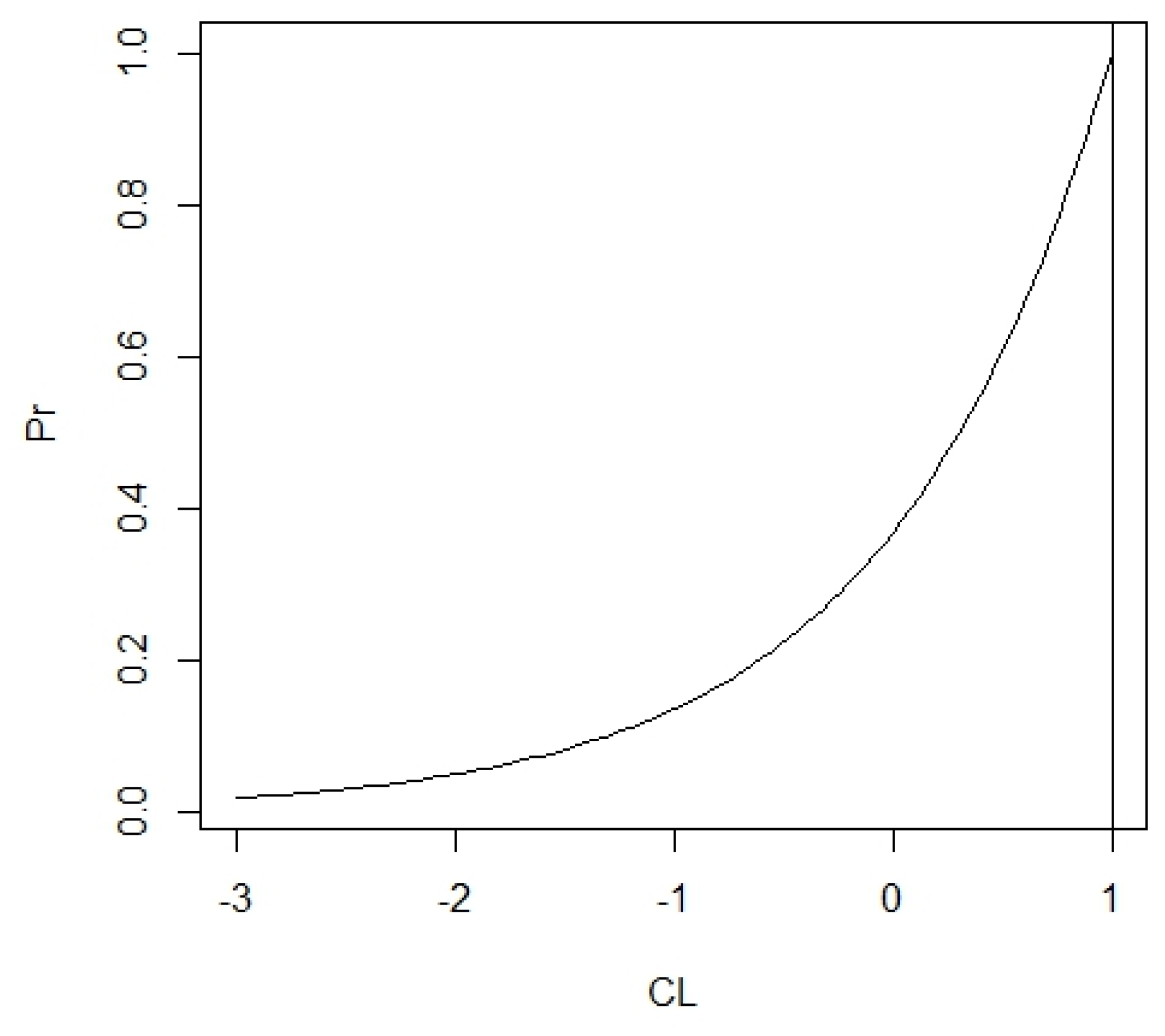
2. The Introduction of the Testing Procedure for the Lifetime Performance Index in Wu [14]
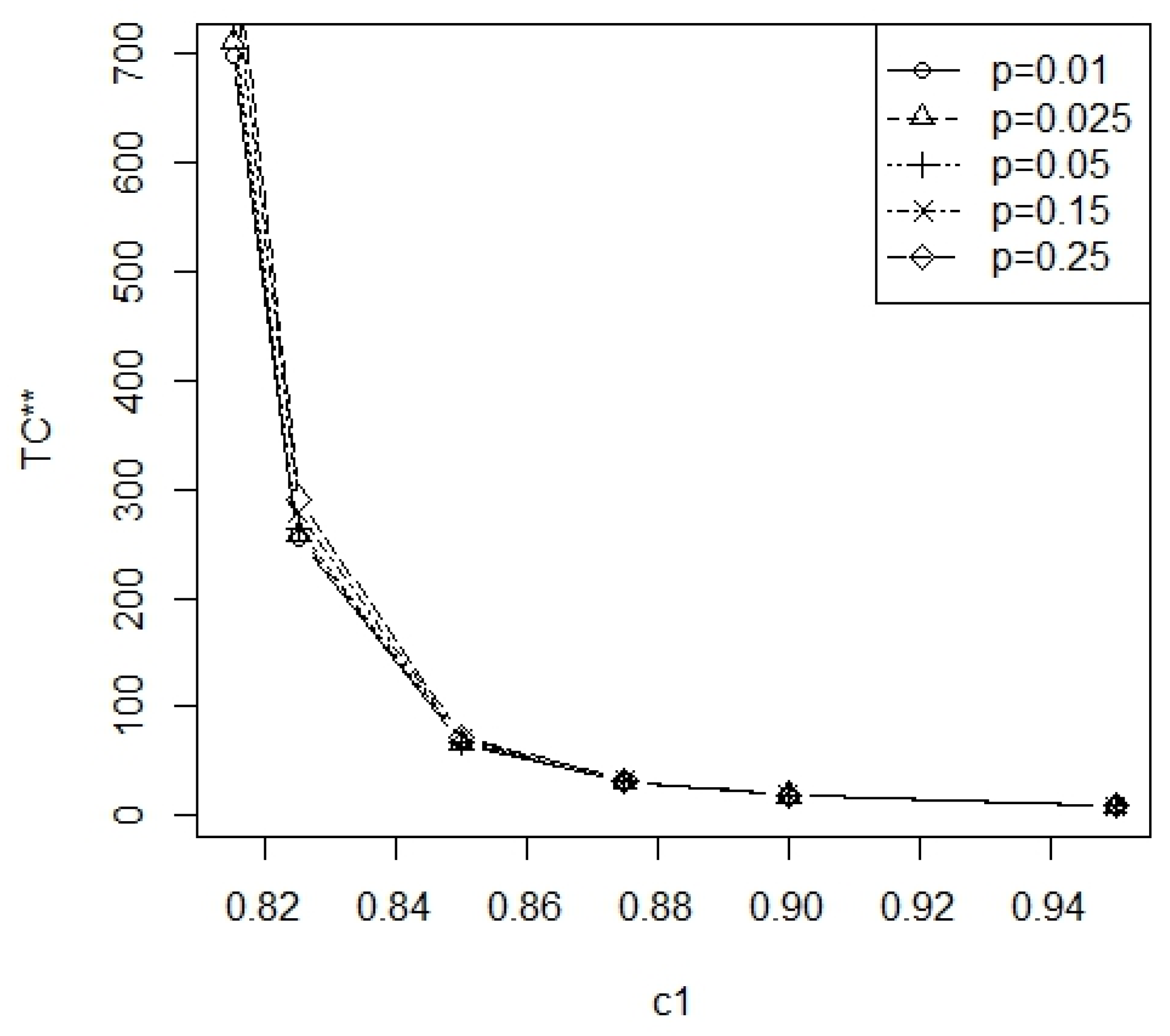
3. Reliability Sampling Design
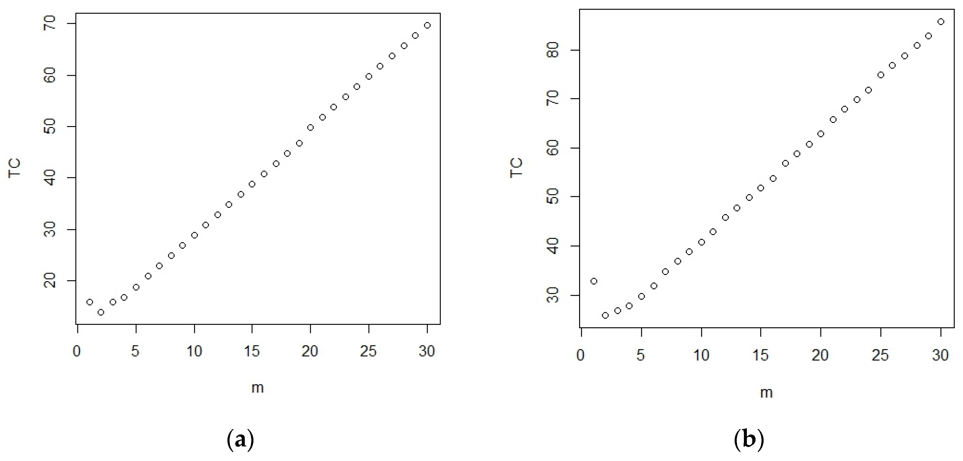
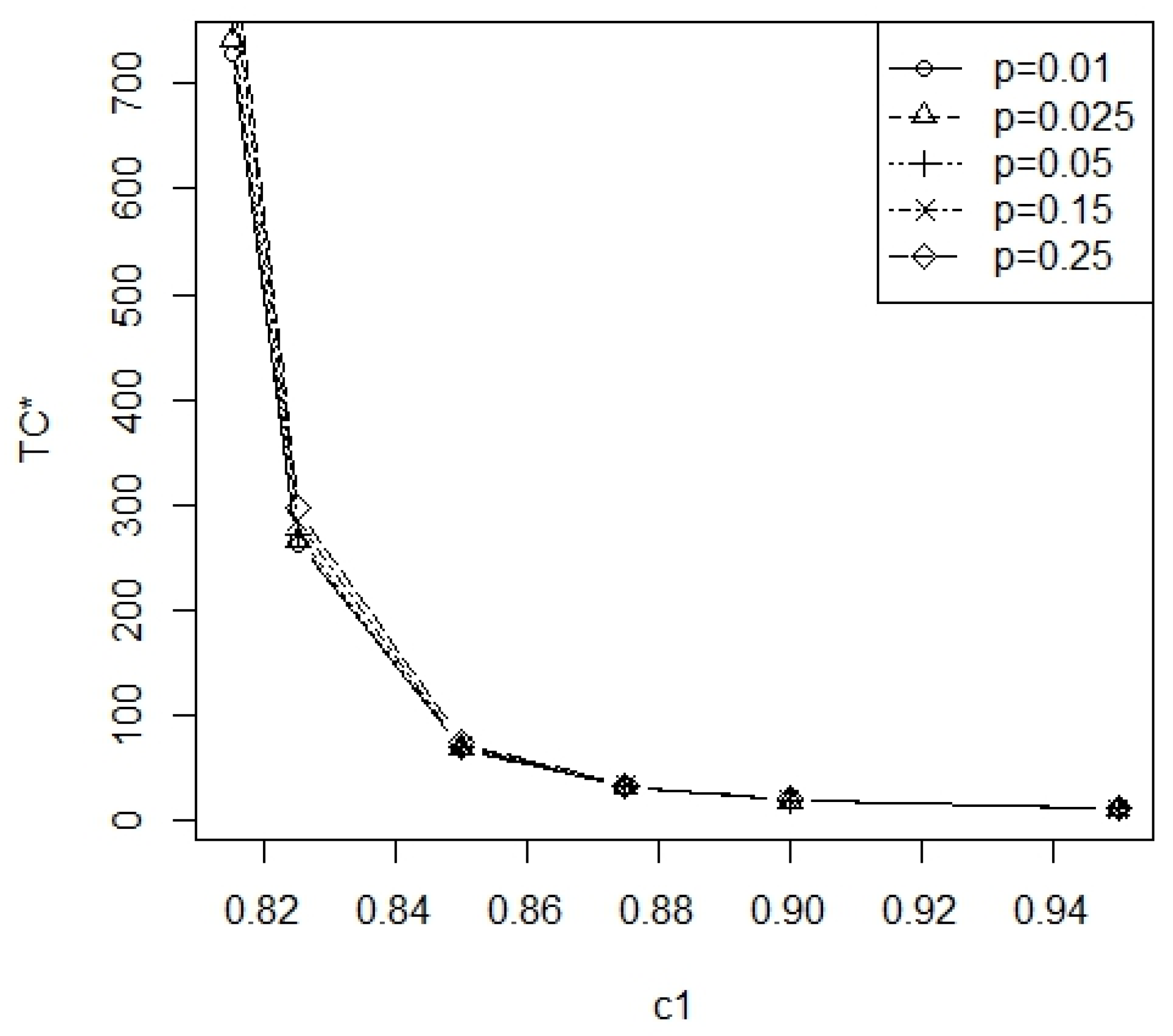
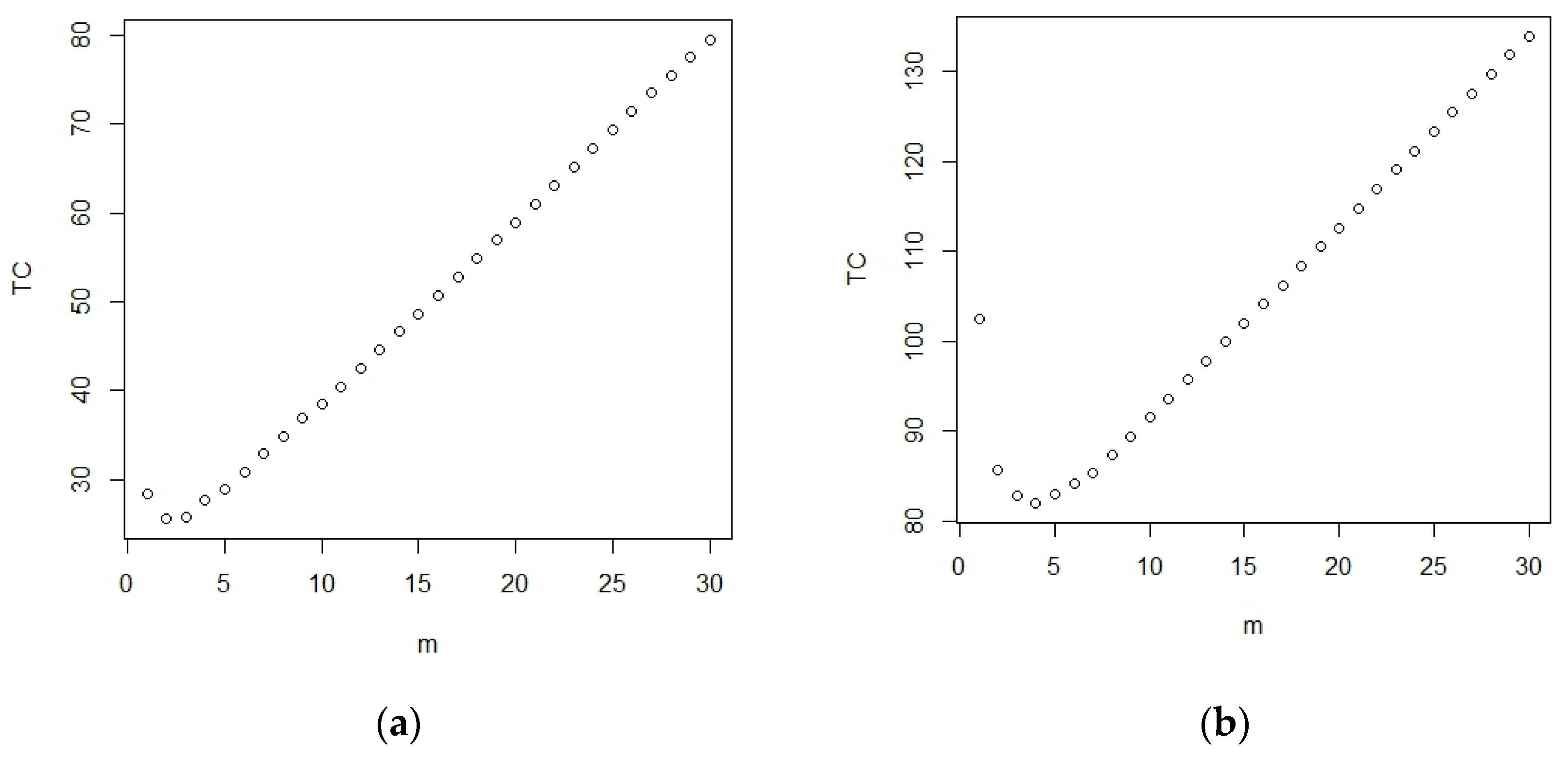
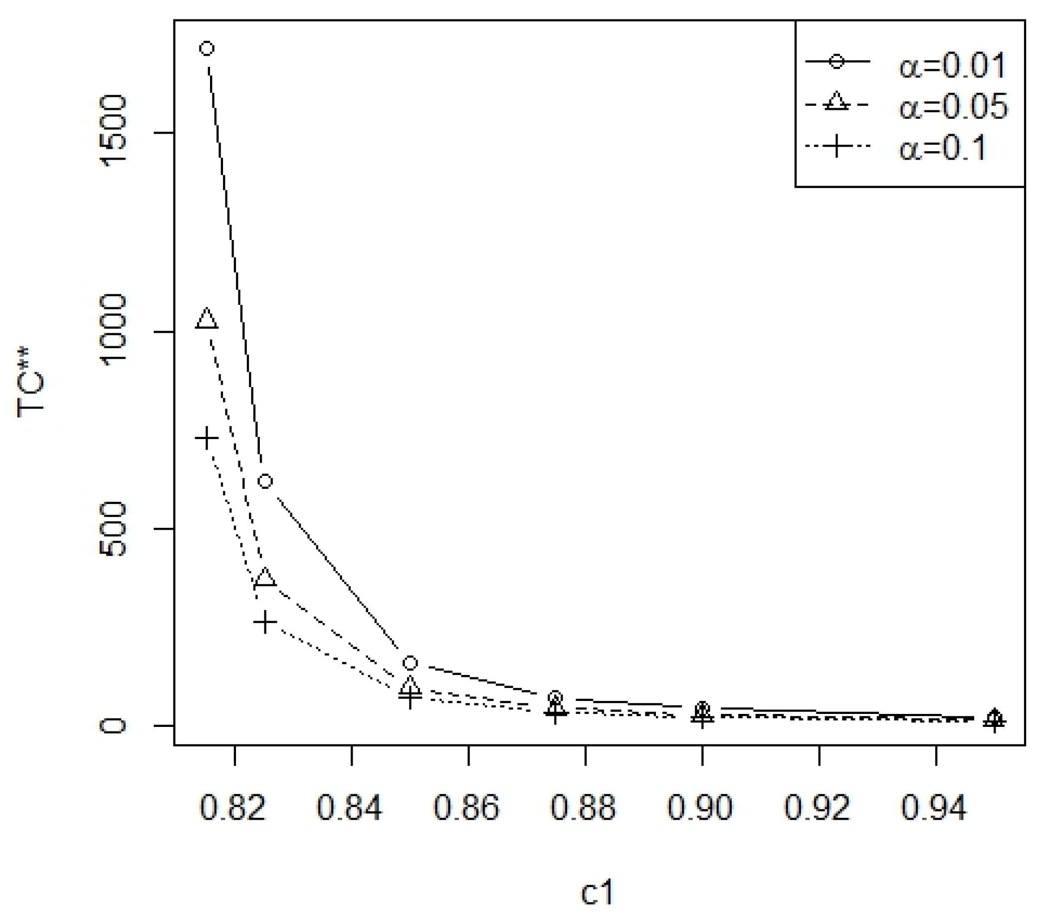
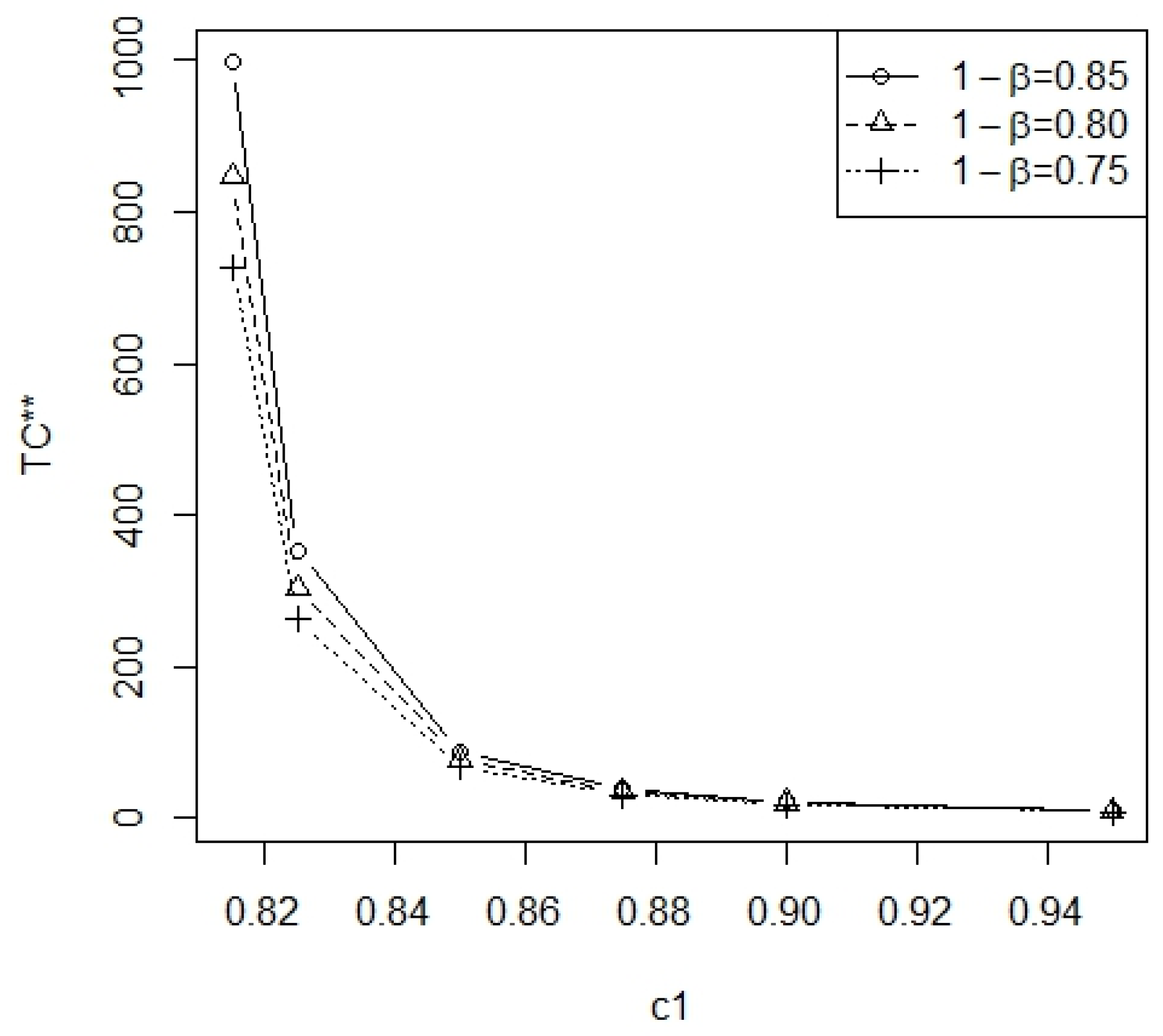
3.1. The Minimal Required m for Fixed T
- Inspection cost CI: the cost for operating a single inspection station;
- Sample cost Cs: the cost for obtaining one unit of sample;
- Operation cost Co: the cost incurred for conducting the experiment per unit of time, which encompasses expenses such as the personnel cost, the depreciation of test equipment, and other related costs.
| Algorithm 1: Utilize the numeration method to search for the optimal (m, n) |
| Step 1: Specify the pre-assigned values of m = 1, c0, c1, α, β, p, T, L, and m0 (the default
value is 30) and CI = aCo, Cs = bCo, Co. Step 2: Compute the sample size n in Equation (11) first and then compute the related total cost TC(m) in Equation (12). Step 3: If m < m0, then m = m + 1 and go to Step 2; otherwise go to Step 4. Step 4: For a array of total costs TC(1),…, TC(m0), The optimal solution of m* is the minimum m value, such that TC(m*) = TC* = TC(m), and then the related sample size n* in Equation (11) is computed. Step 5: Calculate the value of followed by determining the critical value . |
3.2. The minimal Required m, t, and n When the Interval Time of the Experiment Is Unfixed
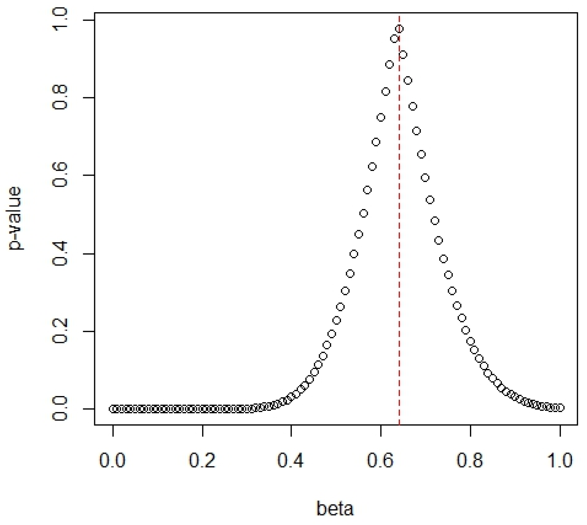
3.3. Example
- Step 1
- Take a random sample of size n = 17 from the data set. Observe the progressive type I interval censored sample (X1,X2) = (4,1) at the pre-set observation time points (t1,t2) = (0.4,0.8) with censoring schemes of (R1,R2) = (1,11).
- Step 2
- Obtain the MLE of k as , and then we can obtain the test statistic = 0.9684447.
- Step 3
- Compare the test statistic with the critical value. We have = 0.9684447 > 0.870090. It can be inferred that the lifetime performance index of product surpasses the required level of 0.80.
- Step 1
- Take a random sample of size n = 17 from the data set. Observe the progressive type I interval censored sample (X1,X2) = (4,1) at the pre-set observation time points (t1,t2) = (0.34,0.68) with censoring schemes of (R1,R2) = (0,12).
- Step 2
- Obtain the MLE of k as , and then we can obtain the test statistic = 0.9694753.
- Step 3
- Comparing the test statistic with the critical value, we have = 0.9694753 > 0.9266319. As a result, we arrived at the same conclusion of rejecting the null hypothesis.
4. Conclusions
Author Contributions
Funding
Data Availability Statement
Conflicts of Interest
Appendix A

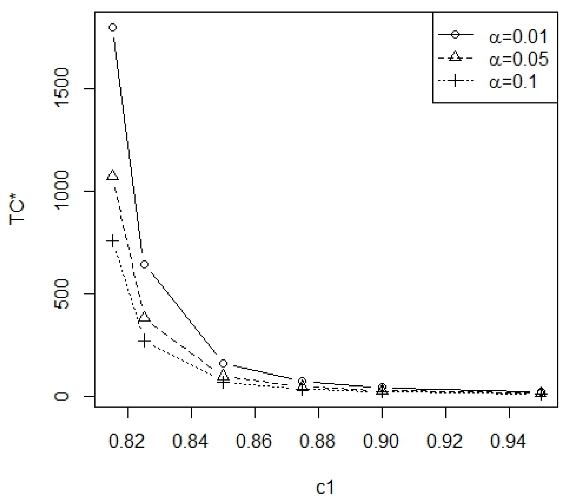
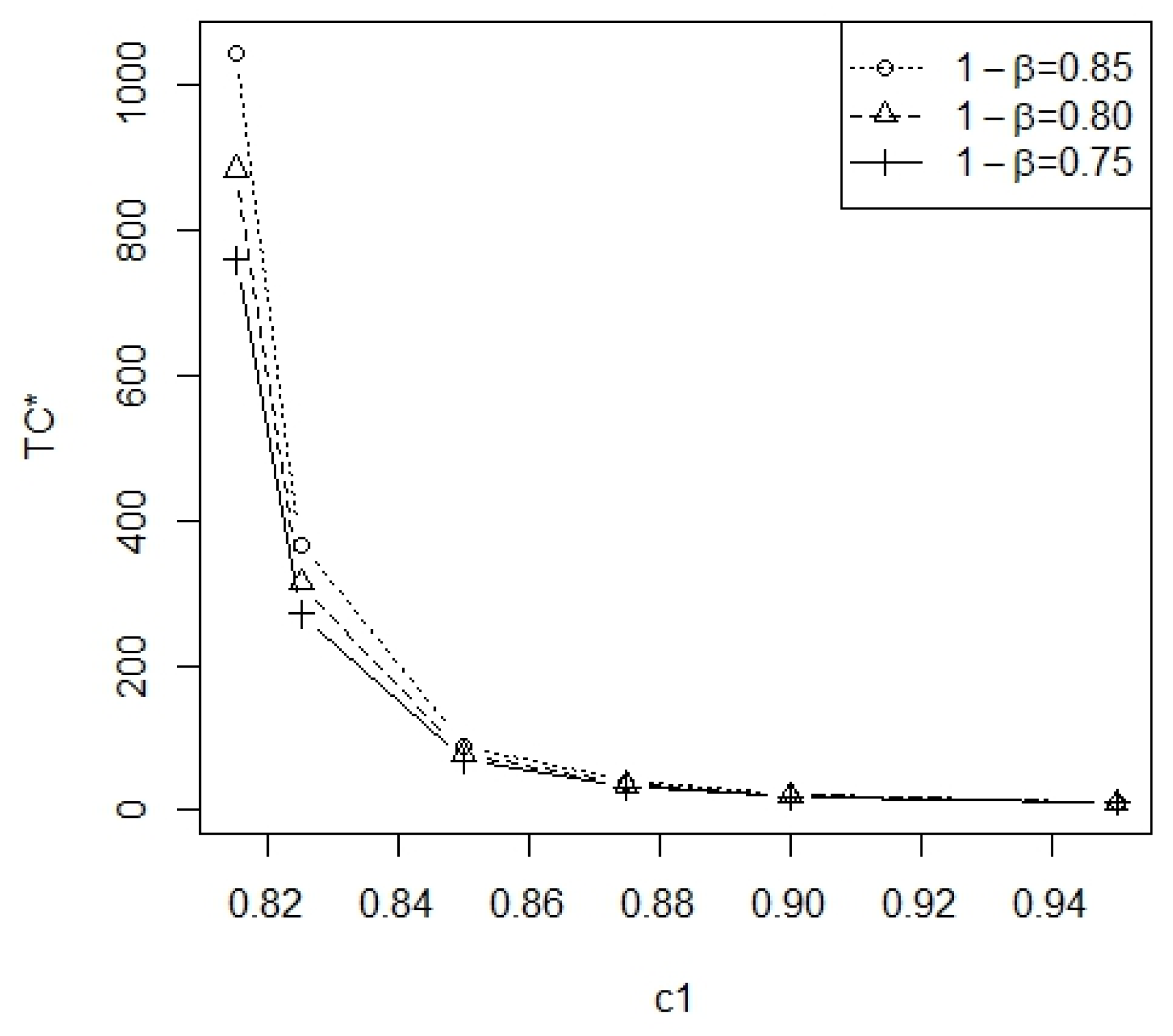
| c1 | 0.825 | 0.85 | ||||||||
|---|---|---|---|---|---|---|---|---|---|---|
| α | β | p | TC* | TC* | ||||||
| 0.01 | 0.25 | 0.010 | 6 | 745 | 757.8 | 0.817927 | 4 | 177 | 185.8 | 0.837169 |
| 0.025 | 5 | 760 | 770.8 | 0.817926 | 4 | 179 | 187.8 | 0.837135 | ||
| 0.050 | 5 | 777 | 787.8 | 0.817918 | 4 | 181 | 189.8 | 0.837218 | ||
| 0.150 | 3 | 828 | 834.8 | 0.817948 | 3 | 193 | 199.8 | 0.837176 | ||
| 0.250 | 3 | 863 | 869.8 | 0.817928 | 3 | 201 | 207.8 | 0.837149 | ||
| 0.20 | 0.010 | 6 | 668 | 680.8 | 0.818932 | 4 | 160 | 168.8 | 0.839094 | |
| 0.025 | 5 | 681 | 691.8 | 0.818937 | 4 | 162 | 170.8 | 0.839035 | ||
| 0.050 | 5 | 696 | 706.8 | 0.818932 | 4 | 165 | 173.8 | 0.838981 | ||
| 0.150 | 3 | 743 | 749.8 | 0.818947 | 3 | 175 | 181.8 | 0.839041 | ||
| 0.250 | 3 | 774 | 780.8 | 0.818931 | 3 | 182 | 188.8 | 0.839040 | ||
| 0.15 | 0.010 | 6 | 605 | 617.8 | 0.819893 | 4 | 147 | 155.8 | 0.840786 | |
| 0.025 | 5 | 617 | 627.8 | 0.819895 | 4 | 148 | 156.8 | 0.840840 | ||
| 0.050 | 5 | 631 | 641.8 | 0.819883 | 4 | 151 | 159.8 | 0.840748 | ||
| 0.150 | 3 | 673 | 679.8 | 0.819908 | 3 | 160 | 166.8 | 0.840830 | ||
| 0.250 | 3 | 701 | 707.8 | 0.819892 | 3 | 167 | 173.8 | 0.840755 | ||
| 0.05 | 0.25 | 0.010 | 6 | 465 | 477.8 | 0.816044 | 4 | 108 | 116.8 | 0.833644 |
| 0.025 | 5 | 474 | 484.8 | 0.816049 | 4 | 109 | 117.8 | 0.833648 | ||
| 0.050 | 4 | 487 | 495.8 | 0.816043 | 3 | 113 | 119.8 | 0.833679 | ||
| 0.150 | 3 | 517 | 523.8 | 0.816060 | 3 | 118 | 124.8 | 0.833617 | ||
| 0.250 | 3 | 538 | 544.8 | 0.816055 | 3 | 123 | 129.8 | 0.833577 | ||
| 0.20 | 0.010 | 5 | 407 | 417.8 | 0.817209 | 4 | 95 | 103.8 | 0.835873 | |
| 0.025 | 5 | 413 | 423.8 | 0.817194 | 4 | 96 | 104.8 | 0.835853 | ||
| 0.050 | 4 | 423 | 431.8 | 0.817214 | 3 | 100 | 106.8 | 0.835801 | ||
| 0.150 | 3 | 450 | 456.8 | 0.817214 | 3 | 104 | 110.8 | 0.835808 | ||
| 0.250 | 3 | 468 | 474.8 | 0.817214 | 3 | 108 | 114.8 | 0.835833 | ||
| 0.15 | 0.010 | 6 | 356 | 368.8 | 0.818336 | 3 | 87 | 93.8 | 0.838078 | |
| 0.025 | 5 | 363 | 373.8 | 0.818340 | 3 | 88 | 94.8 | 0.837975 | ||
| 0.050 | 4 | 373 | 381.8 | 0.818331 | 3 | 89 | 95.8 | 0.837949 | ||
| 0.150 | 3 | 396 | 402.8 | 0.818350 | 3 | 93 | 99.8 | 0.837866 | ||
| 0.250 | 3 | 412 | 418.8 | 0.818346 | 2 | 99 | 103.8 | 0.838114 | ||
| 0.10 | 0.25 | 0.010 | 5 | 345 | 355.8 | 0.814563 | 3 | 81 | 87.8 | 0.830747 |
| 0.025 | 5 | 350 | 360.8 | 0.814552 | 3 | 81 | 87.8 | 0.830839 | ||
| 0.050 | 4 | 358 | 366.8 | 0.814578 | 3 | 82 | 88.8 | 0.830804 | ||
| 0.150 | 3 | 381 | 387.8 | 0.814576 | 3 | 86 | 92.8 | 0.830680 | ||
| 0.250 | 3 | 397 | 403.8 | 0.814562 | 2 | 91 | 95.8 | 0.830973 | ||
| 0.20 | 0.010 | 5 | 293 | 303.8 | 0.815803 | 3 | 69 | 75.8 | 0.833314 | |
| 0.025 | 5 | 297 | 307.8 | 0.815797 | 3 | 70 | 76.8 | 0.833174 | ||
| 0.050 | 4 | 305 | 313.8 | 0.815794 | 3 | 71 | 77.8 | 0.833104 | ||
| 0.150 | 3 | 323 | 329.8 | 0.815831 | 3 | 74 | 80.8 | 0.833074 | ||
| 0.250 | 3 | 337 | 343.8 | 0.815805 | 2 | 78 | 82.8 | 0.833455 | ||
| 0.15 | 0.010 | 5 | 252 | 262.8 | 0.817040 | 3 | 61 | 67.8 | 0.835431 | |
| 0.025 | 5 | 255 | 265.8 | 0.817049 | 3 | 61 | 67.8 | 0.835537 | ||
| 0.050 | 4 | 262 | 270.8 | 0.817041 | 3 | 62 | 68.8 | 0.835425 | ||
| 0.150 | 3 | 278 | 284.8 | 0.817064 | 3 | 64 | 70.8 | 0.835564 | ||
| 0.250 | 3 | 290 | 296.8 | 0.817037 | 2 | 69 | 73.8 | 0.835570 |
| c1 | 0.875 | 0.90 | ||||||||
|---|---|---|---|---|---|---|---|---|---|---|
| α | β | p | TC* | TC* | ||||||
| 0.01 | 0.25 | 0.010 | 3 | 75 | 81.8 | 0.858004 | 3 | 39 | 45.8 | 0.880437 |
| 0.025 | 3 | 76 | 82.8 | 0.857793 | 3 | 40 | 46.8 | 0.879663 | ||
| 0.050 | 3 | 76 | 82.8 | 0.858082 | 3 | 40 | 46.8 | 0.880060 | ||
| 0.150 | 3 | 80 | 86.8 | 0.857743 | 2 | 44 | 48.8 | 0.880105 | ||
| 0.250 | 2 | 85 | 89.8 | 0.858175 | 2 | 45 | 49.8 | 0.879954 | ||
| 0.20 | 0.010 | 3 | 69 | 75.8 | 0.860473 | 2 | 39 | 43.8 | 0.884001 | |
| 0.025 | 3 | 69 | 75.8 | 0.860654 | 3 | 37 | 43.8 | 0.882829 | ||
| 0.050 | 3 | 70 | 76.8 | 0.860520 | 3 | 37 | 43.8 | 0.883242 | ||
| 0.150 | 3 | 73 | 79.8 | 0.860448 | 2 | 41 | 45.8 | 0.882984 | ||
| 0.250 | 2 | 78 | 82.8 | 0.860730 | 2 | 41 | 45.8 | 0.883764 | ||
| 0.15 | 0.010 | 3 | 64 | 70.8 | 0.862791 | 3 | 34 | 40.8 | 0.886148 | |
| 0.025 | 3 | 64 | 70.8 | 0.862979 | 2 | 37 | 41.8 | 0.886359 | ||
| 0.050 | 3 | 65 | 71.8 | 0.862804 | 2 | 37 | 41.8 | 0.886555 | ||
| 0.150 | 3 | 68 | 74.8 | 0.862631 | 2 | 38 | 42.8 | 0.886197 | ||
| 0.250 | 2 | 72 | 76.8 | 0.863210 | 2 | 39 | 43.8 | 0.885885 | ||
| 0.05 | 0.25 | 0.010 | 3 | 45 | 51.8 | 0.852946 | 2 | 25 | 29.8 | 0.874182 |
| 0.025 | 3 | 45 | 51.8 | 0.853104 | 2 | 25 | 29.8 | 0.874283 | ||
| 0.050 | 3 | 46 | 52.8 | 0.852786 | 2 | 25 | 29.8 | 0.874452 | ||
| 0.150 | 2 | 50 | 54.8 | 0.853131 | 2 | 26 | 30.8 | 0.873680 | ||
| 0.250 | 2 | 51 | 55.8 | 0.853103 | 2 | 26 | 30.8 | 0.874373 | ||
| 0.20 | 0.010 | 3 | 40 | 46.8 | 0.856158 | 2 | 23 | 27.8 | 0.877341 | |
| 0.025 | 2 | 43 | 47.8 | 0.856640 | 2 | 23 | 27.8 | 0.877446 | ||
| 0.050 | 3 | 41 | 47.8 | 0.855912 | 2 | 23 | 27.8 | 0.877622 | ||
| 0.150 | 2 | 45 | 49.8 | 0.856005 | 2 | 23 | 27.8 | 0.878338 | ||
| 0.250 | 2 | 46 | 50.8 | 0.855914 | 2 | 24 | 28.8 | 0.877410 | ||
| 0.15 | 0.010 | 3 | 36 | 42.8 | 0.859195 | 2 | 21 | 25.8 | 0.880940 | |
| 0.025 | 2 | 39 | 43.8 | 0.859474 | 2 | 21 | 25.8 | 0.881050 | ||
| 0.050 | 3 | 37 | 43.8 | 0.858857 | 2 | 21 | 25.8 | 0.881234 | ||
| 0.150 | 2 | 40 | 44.8 | 0.859403 | 2 | 21 | 25.8 | 0.881984 | ||
| 0.250 | 2 | 41 | 45.8 | 0.859226 | 2 | 22 | 26.8 | 0.880852 | ||
| 0.10 | 0.25 | 0.010 | 2 | 34 | 38.8 | 0.849561 | 2 | 17 | 21.8 | 0.870090 |
| 0.025 | 3 | 32 | 38.8 | 0.849065 | 2 | 17 | 21.8 | 0.870185 | ||
| 0.050 | 2 | 35 | 39.8 | 0.849025 | 2 | 18 | 22.8 | 0.868363 | ||
| 0.150 | 2 | 35 | 39.8 | 0.849478 | 2 | 18 | 22.8 | 0.868994 | ||
| 0.250 | 2 | 36 | 40.8 | 0.849245 | 2 | 18 | 22.8 | 0.869642 | ||
| 0.20 | 0.010 | 2 | 30 | 34.8 | 0.852762 | 2 | 16 | 20.8 | 0.872247 | |
| 0.025 | 2 | 30 | 34.8 | 0.852833 | 2 | 16 | 20.8 | 0.872345 | ||
| 0.050 | 2 | 31 | 35.8 | 0.852092 | 2 | 16 | 20.8 | 0.872510 | ||
| 0.150 | 2 | 31 | 35.8 | 0.852573 | 2 | 16 | 20.8 | 0.873179 | ||
| 0.250 | 2 | 32 | 36.8 | 0.852232 | 2 | 16 | 20.8 | 0.873867 | ||
| 0.15 | 0.010 | 2 | 27 | 31.8 | 0.855616 | 2 | 14 | 18.8 | 0.877235 | |
| 0.025 | 2 | 27 | 31.8 | 0.855691 | 2 | 14 | 18.8 | 0.877340 | ||
| 0.050 | 2 | 27 | 31.8 | 0.855818 | 2 | 14 | 18.8 | 0.877516 | ||
| 0.150 | 2 | 28 | 32.8 | 0.855318 | 2 | 15 | 19.8 | 0.875579 | ||
| 0.250 | 2 | 28 | 32.8 | 0.855838 | 2 | 15 | 19.8 | 0.876289 |
| c1 | 0.825 | 0.85 | ||||||||||
|---|---|---|---|---|---|---|---|---|---|---|---|---|
| α | β | p | ||||||||||
| 0.01 | 0.15 | 0.010 | 10 | 0.14 | 702 | 723.36 | 0.817978 | 6 | 0.18 | 167 | 180.08 | 0.837372 |
| 0.025 | 8 | 0.17 | 719 | 736.38 | 0.817985 | 5 | 0.21 | 171 | 182.07 | 0.837391 | ||
| 0.050 | 7 | 0.20 | 739 | 754.37 | 0.817982 | 5 | 0.22 | 174 | 185.09 | 0.837367 | ||
| 0.150 | 5 | 0.27 | 796 | 807.34 | 0.817984 | 4 | 0.27 | 186 | 195.09 | 0.837368 | ||
| 0.250 | 5 | 0.29 | 836 | 847.44 | 0.817973 | 4 | 0.31 | 194 | 203.24 | 0.837387 | ||
| 0.20 | 0.010 | 9 | 0.15 | 632 | 651.34 | 0.818984 | 6 | 0.20 | 151 | 164.18 | 0.839282 | |
| 0.025 | 9 | 0.16 | 643 | 662.43 | 0.818983 | 5 | 0.22 | 155 | 166.10 | 0.839262 | ||
| 0.050 | 7 | 0.20 | 663 | 678.38 | 0.818985 | 5 | 0.21 | 158 | 169.07 | 0.839238 | ||
| 0.150 | 6 | 0.25 | 712 | 725.50 | 0.818980 | 4 | 0.27 | 169 | 178.06 | 0.839203 | ||
| 0.250 | 5 | 0.29 | 750 | 761.44 | 0.818975 | 4 | 0.31 | 176 | 185.26 | 0.839252 | ||
| 0.25 | 0.010 | 9 | 0.15 | 573 | 592.35 | 0.819937 | 5 | 0.20 | 141 | 152.01 | 0.840983 | |
| 0.025 | 8 | 0.17 | 585 | 602.38 | 0.819938 | 5 | 0.22 | 142 | 153.12 | 0.841020 | ||
| 0.050 | 7 | 0.18 | 602 | 617.30 | 0.819938 | 5 | 0.21 | 145 | 156.04 | 0.840959 | ||
| 0.150 | 5 | 0.26 | 648 | 659.28 | 0.819930 | 4 | 0.26 | 155 | 164.04 | 0.840953 | ||
| 0.250 | 5 | 0.29 | 680 | 691.43 | 0.819928 | 3 | 0.31 | 164 | 170.92 | 0.840931 | ||
| 0.05 | 0.15 | 0.010 | 8 | 0.16 | 441 | 458.30 | 0.816111 | 5 | 0.22 | 103 | 114.09 | 0.833883 |
| 0.025 | 8 | 0.17 | 448 | 465.36 | 0.816109 | 5 | 0.23 | 104 | 115.14 | 0.833897 | ||
| 0.050 | 6 | 0.21 | 463 | 476.28 | 0.816111 | 4 | 0.25 | 108 | 117.00 | 0.833837 | ||
| 0.150 | 5 | 0.26 | 496 | 507.32 | 0.816107 | 3 | 0.30 | 116 | 122.91 | 0.833820 | ||
| 0.250 | 4 | 0.30 | 523 | 532.19 | 0.816098 | 3 | 0.33 | 120 | 126.98 | 0.833832 | ||
| 0.20 | 0.010 | 8 | 0.16 | 384 | 401.30 | 0.817265 | 5 | 0.21 | 91 | 102.06 | 0.836050 | |
| 0.025 | 8 | 0.17 | 390 | 407.39 | 0.817266 | 4 | 0.24 | 94 | 102.98 | 0.836036 | ||
| 0.050 | 7 | 0.19 | 401 | 416.35 | 0.817262 | 4 | 0.23 | 96 | 104.90 | 0.835931 | ||
| 0.150 | 5 | 0.26 | 432 | 443.30 | 0.817259 | 4 | 0.28 | 100 | 109.12 | 0.836031 | ||
| 0.250 | 4 | 0.31 | 455 | 464.23 | 0.817261 | 3 | 0.32 | 106 | 112.95 | 0.835992 | ||
| 0.25 | 0.010 | 7 | 0.17 | 341 | 356.19 | 0.818390 | 4 | 0.21 | 84 | 92.85 | 0.838071 | |
| 0.025 | 7 | 0.17 | 346 | 361.22 | 0.818393 | 4 | 0.24 | 84 | 92.95 | 0.838121 | ||
| 0.050 | 7 | 0.20 | 353 | 368.41 | 0.818396 | 4 | 0.25 | 85 | 94.00 | 0.838141 | ||
| 0.150 | 5 | 0.25 | 381 | 392.24 | 0.818381 | 3 | 0.27 | 92 | 98.82 | 0.838054 | ||
| 0.250 | 4 | 0.30 | 401 | 410.19 | 0.818384 | 3 | 0.30 | 95 | 101.89 | 0.838044 | ||
| 0.10 | 0.15 | 0.010 | 7 | 0.17 | 327 | 342.20 | 0.814632 | 4 | 0.22 | 77 | 85.89 | 0.830936 |
| 0.025 | 7 | 0.17 | 332 | 347.21 | 0.814629 | 4 | 0.25 | 77 | 85.99 | 0.831018 | ||
| 0.050 | 6 | 0.20 | 341 | 354.22 | 0.814630 | 4 | 0.26 | 78 | 87.02 | 0.831024 | ||
| 0.150 | 5 | 0.26 | 365 | 376.30 | 0.814629 | 3 | 0.30 | 84 | 90.90 | 0.830965 | ||
| 0.250 | 4 | 0.29 | 385 | 394.18 | 0.814621 | 3 | 0.32 | 87 | 93.95 | 0.830953 | ||
| 0.20 | 0.010 | 7 | 0.17 | 278 | 293.20 | 0.815869 | 4 | 0.24 | 66 | 74.95 | 0.833370 | |
| 0.025 | 6 | 0.20 | 284 | 297.22 | 0.815874 | 3 | 0.29 | 69 | 75.87 | 0.833391 | ||
| 0.050 | 6 | 0.20 | 290 | 303.21 | 0.815865 | 3 | 0.27 | 70 | 76.82 | 0.833330 | ||
| 0.150 | 4 | 0.28 | 313 | 322.12 | 0.815868 | 3 | 0.28 | 73 | 79.83 | 0.833249 | ||
| 0.250 | 4 | 0.30 | 327 | 336.20 | 0.815862 | 3 | 0.32 | 75 | 81.95 | 0.833338 | ||
| 0.25 | 0.010 | 7 | 0.18 | 239 | 254.23 | 0.817112 | 3 | 0.28 | 60 | 66.83 | 0.835706 | |
| 0.025 | 6 | 0.19 | 245 | 258.11 | 0.817096 | 4 | 0.24 | 58 | 66.97 | 0.835744 | ||
| 0.050 | 5 | 0.22 | 252 | 263.10 | 0.817105 | 3 | 0.28 | 61 | 67.83 | 0.835685 | ||
| 0.150 | 5 | 0.26 | 267 | 278.28 | 0.817104 | 3 | 0.32 | 63 | 69.95 | 0.835767 | ||
| 0.250 | 4 | 0.28 | 282 | 291.13 | 0.817093 | 3 | 0.29 | 66 | 72.86 | 0.835591 | ||
| c1 | 0.875 | 0.90 | ||||||||||
|---|---|---|---|---|---|---|---|---|---|---|---|---|
| α | β | p | ||||||||||
| 0.01 | 0.15 | 0.010 | 4 | 0.21 | 72 | 80.86 | 0.858158 | 3 | 0.26 | 39 | 45.78 | 0.880480 |
| 0.025 | 4 | 0.24 | 72 | 80.95 | 0.858235 | 3 | 0.28 | 39 | 45.83 | 0.880627 | ||
| 0.050 | 4 | 0.24 | 73 | 81.96 | 0.858230 | 3 | 0.25 | 40 | 46.74 | 0.880226 | ||
| 0.150 | 3 | 0.28 | 79 | 85.83 | 0.858019 | 3 | 0.29 | 41 | 47.86 | 0.880481 | ||
| 0.250 | 3 | 0.33 | 81 | 87.98 | 0.858239 | 2 | 0.31 | 45 | 49.63 | 0.880063 | ||
| 0.20 | 0.010 | 4 | 0.22 | 66 | 74.86 | 0.860656 | 3 | 0.28 | 36 | 42.83 | 0.883677 | |
| 0.025 | 4 | 0.24 | 66 | 74.96 | 0.860825 | 3 | 0.23 | 37 | 43.70 | 0.883314 | ||
| 0.050 | 4 | 0.24 | 67 | 75.96 | 0.860781 | 3 | 0.25 | 37 | 43.76 | 0.883415 | ||
| 0.150 | 3 | 0.29 | 72 | 78.88 | 0.860732 | 3 | 0.29 | 38 | 44.87 | 0.883598 | ||
| 0.250 | 3 | 0.29 | 75 | 81.87 | 0.860607 | 2 | 0.37 | 41 | 45.74 | 0.883592 | ||
| 0.25 | 0.010 | 4 | 0.22 | 61 | 69.88 | 0.863093 | 3 | 0.25 | 34 | 40.75 | 0.886296 | |
| 0.025 | 3 | 0.26 | 64 | 70.77 | 0.863016 | 3 | 0.27 | 34 | 40.80 | 0.886387 | ||
| 0.050 | 4 | 0.24 | 62 | 70.97 | 0.863185 | 2 | 0.32 | 37 | 41.65 | 0.886264 | ||
| 0.150 | 3 | 0.28 | 67 | 73.83 | 0.863001 | 2 | 0.31 | 38 | 42.63 | 0.886147 | ||
| 0.250 | 3 | 0.31 | 69 | 75.93 | 0.863103 | 2 | 0.31 | 39 | 43.62 | 0.886001 | ||
| 0.05 | 0.15 | 0.010 | 3 | 0.25 | 45 | 51.75 | 0.853037 | 2 | 0.30 | 25 | 29.61 | 0.874037 |
| 0.025 | 3 | 0.26 | 45 | 51.78 | 0.853136 | 2 | 0.31 | 25 | 29.62 | 0.874068 | ||
| 0.050 | 3 | 0.29 | 45 | 51.87 | 0.853318 | 2 | 0.32 | 25 | 29.64 | 0.874201 | ||
| 0.150 | 3 | 0.29 | 47 | 53.86 | 0.853148 | 2 | 0.30 | 26 | 30.59 | 0.873748 | ||
| 0.250 | 2 | 0.34 | 51 | 55.68 | 0.853011 | 2 | 0.34 | 26 | 30.69 | 0.874244 | ||
| 0.20 | 0.010 | 3 | 0.26 | 40 | 46.77 | 0.856188 | 2 | 0.28 | 23 | 27.55 | 0.877466 | |
| 0.025 | 3 | 0.27 | 40 | 46.82 | 0.856313 | 2 | 0.28 | 23 | 27.56 | 0.877600 | ||
| 0.050 | 3 | 0.25 | 41 | 47.74 | 0.856028 | 2 | 0.29 | 23 | 27.58 | 0.877662 | ||
| 0.150 | 3 | 0.29 | 42 | 48.86 | 0.856223 | 2 | 0.34 | 23 | 27.68 | 0.878102 | ||
| 0.250 | 2 | 0.31 | 46 | 50.63 | 0.855990 | 2 | 0.30 | 24 | 28.61 | 0.877649 | ||
| 0.25 | 0.010 | 3 | 0.27 | 36 | 42.80 | 0.859184 | 2 | 0.28 | 21 | 25.55 | 0.881071 | |
| 0.025 | 2 | 0.34 | 39 | 43.68 | 0.859205 | 2 | 0.28 | 21 | 25.56 | 0.881211 | ||
| 0.050 | 3 | 0.25 | 37 | 43.74 | 0.858979 | 2 | 0.29 | 21 | 25.58 | 0.881276 | ||
| 0.150 | 2 | 0.35 | 40 | 44.71 | 0.859213 | 2 | 0.35 | 21 | 25.70 | 0.881722 | ||
| 0.250 | 2 | 0.35 | 41 | 45.69 | 0.859100 | 2 | 0.30 | 22 | 26.59 | 0.881101 | ||
| 0.10 | 0.15 | 0.010 | 2 | 0.37 | 34 | 38.75 | 0.849386 | 2 | 0.37 | 17 | 21.74 | 0.869842 |
| 0.025 | 3 | 0.26 | 32 | 38.79 | 0.849094 | 2 | 0.27 | 18 | 22.54 | 0.868511 | ||
| 0.050 | 3 | 0.29 | 32 | 38.86 | 0.849262 | 2 | 0.28 | 18 | 22.56 | 0.868540 | ||
| 0.150 | 2 | 0.39 | 35 | 39.78 | 0.849421 | 2 | 0.31 | 18 | 22.63 | 0.868954 | ||
| 0.250 | 2 | 0.36 | 36 | 40.72 | 0.849135 | 2 | 0.37 | 18 | 22.74 | 0.869499 | ||
| 0.20 | 0.010 | 2 | 0.34 | 30 | 34.67 | 0.852513 | 2 | 0.26 | 16 | 20.52 | 0.872750 | |
| 0.025 | 2 | 0.35 | 30 | 34.70 | 0.852598 | 2 | 0.27 | 16 | 20.53 | 0.872667 | ||
| 0.050 | 3 | 0.29 | 28 | 34.87 | 0.852663 | 2 | 0.27 | 16 | 20.55 | 0.872881 | ||
| 0.150 | 2 | 0.34 | 31 | 35.67 | 0.852415 | 2 | 0.31 | 16 | 20.62 | 0.873136 | ||
| 0.250 | 2 | 0.32 | 32 | 36.64 | 0.852231 | 2 | 0.37 | 16 | 20.73 | 0.873715 | ||
| 0.25 | 0.010 | 2 | 0.29 | 27 | 31.59 | 0.855595 | 2 | 0.29 | 14 | 18.58 | 0.877207 | |
| 0.025 | 2 | 0.30 | 27 | 31.60 | 0.855599 | 2 | 0.30 | 14 | 18.59 | 0.877212 | ||
| 0.050 | 2 | 0.31 | 27 | 31.63 | 0.855682 | 2 | 0.31 | 14 | 18.62 | 0.877327 | ||
| 0.150 | 2 | 0.29 | 28 | 32.58 | 0.855473 | 1 | 0.43 | 17 | 19.43 | 0.877249 | ||
| 0.250 | 2 | 0.34 | 28 | 32.68 | 0.855741 | 1 | 0.43 | 17 | 19.43 | 0.877249 | ||
References
- Montgomery, D.C. Introduction to Statistical Quality Control; John Wiley and Sons Inc.: New York, NY, USA, 1985. [Google Scholar]
- Balakrishnan, N.; Aggarwala, R. Progressive Censoring: Theory, Methods and Applications; Birkhäuser: Boston, MA, USA, 2000. [Google Scholar]
- Aggarwala, R. Progressive interval censoring: Some mathematical results with applications to inference. Commun. Stat.-Theory Methods 2001, 30, 1921–1935. [Google Scholar]
- Balakrishnan, N. Progressive Censoring Methodology: An Appraisal (with Discussions). Test 2007, 16, 211–296. [Google Scholar] [CrossRef]
- Balakrishnan, N.; Cramer, E. The Art of Progressive Censoring; Birkhäuser: Boston, MA, USA, 2014. [Google Scholar]
- Laumen, B.; Cramer, E. Inference for the lifetime performance index with progressively Type-II censored samples from gamma distributions. Econ. Qual. Control 2015, 30, 59–73. [Google Scholar] [CrossRef]
- Bdair, O.M.; Abu Awwad, R.R.; Abufoudeh, G.K.; Naser, M.F.M. Estimation and Prediction for Flexible Weibull Distribution Based on Progressive Type II Censored Data. Commun. Math. Stat. 2020, 8, 255–277. [Google Scholar] [CrossRef]
- Panahi, H. Interval estimation of Kumaraswamy parameters based on progressively type II censored sample and record values. Miskolc Math. Notes 2020, 21, 319. [Google Scholar] [CrossRef]
- EL-Sagheer, R.M. Estimation of parameters of Weibull–Gamma distribution based on progressively censored data. Stat. Pap. 2018, 59, 725–757. [Google Scholar] [CrossRef] [Green Version]
- Lee, W.C.; Wu, J.W.; Hong, C.W. Assessing the lifetime performance index of products with the exponential distribution under progressively type II right censored samples. J. Comput. Appl. Math. 2009, 231, 648–656. [Google Scholar] [CrossRef] [Green Version]
- Wu, J.W.; Lee, W.C.; Lin, L.S.; Hong, M.L. Bayesian test of lifetime performance index for exponential products based on the progressively type II right censored sample. J. Quant. Manag. 2011, 8, 57–77. [Google Scholar]
- Wu, S.F.; Lin, Y.P. Computational testing algorithmic procedure of assessment for lifetime performance index of products with one-parameter exponential distribution under progressive type I interval censoring. Math. Comput. Simul. 2016, 120, 79–90. [Google Scholar] [CrossRef]
- Wu, S.F.; Liu, T.H.; Lai, Y.H.; Chang, W.T. A study on the experimental design for the lifetime performance index of Rayleigh lifetime distribution under progressive type I interval censoring. Mathematics 2022, 10, 517. [Google Scholar] [CrossRef]
- Wu, S.F. The performance assessment on the lifetime performance index of products following Chen lifetime distribution based on the progressive type I interval censored sample. J. Comput. Appl. Math. 2018, 334, 27–38. [Google Scholar] [CrossRef]
- Chen, Z. A new two-parameter lifetime distribution with bathtub shape or increasing failure rate function. Stat. Probab. Lett. 2000, 49, 155–161. [Google Scholar] [CrossRef]
- Huang, S.R.; Wu, S.J. Reliability sampling plans under progressive type-I interval censoring using cost functions. IEEE Trans. Reliab. 2008, 57, 445–451. [Google Scholar] [CrossRef]
- Xie, M.; Lai, C.D. Reliability analysis using an additiveWeibull model with bathtub-shaped failure rate function. Reliab. Eng. Syst. Saf. 1995, 52, 87–93. [Google Scholar] [CrossRef]
- Gail, M.H.; Gastwirth, J.L. A scale-free goodness of fit test for the exponential distribution based on the Gini Statistic. J. R. Stat. Soc. B 1978, 40, 350–357. [Google Scholar] [CrossRef]


Disclaimer/Publisher’s Note: The statements, opinions and data contained in all publications are solely those of the individual author(s) and contributor(s) and not of MDPI and/or the editor(s). MDPI and/or the editor(s) disclaim responsibility for any injury to people or property resulting from any ideas, methods, instructions or products referred to in the content. |
© 2023 by the authors. Licensee MDPI, Basel, Switzerland. This article is an open access article distributed under the terms and conditions of the Creative Commons Attribution (CC BY) license (https://creativecommons.org/licenses/by/4.0/).
Share and Cite
Wu, S.-F.; Song, M.-Z. Experimental Design for Progressive Type I Interval Censoring on the Lifetime Performance Index of Chen Lifetime Distribution. Mathematics 2023, 11, 1554. https://doi.org/10.3390/math11061554
Wu S-F, Song M-Z. Experimental Design for Progressive Type I Interval Censoring on the Lifetime Performance Index of Chen Lifetime Distribution. Mathematics. 2023; 11(6):1554. https://doi.org/10.3390/math11061554
Chicago/Turabian StyleWu, Shu-Fei, and Meng-Zong Song. 2023. "Experimental Design for Progressive Type I Interval Censoring on the Lifetime Performance Index of Chen Lifetime Distribution" Mathematics 11, no. 6: 1554. https://doi.org/10.3390/math11061554