Robust Optimal Investment Strategies with Exchange Rate Risk and Default Risk

Abstract

The problem of robust optimal investment with exchange rate risk and default risk is studied. We assume that investors are ambiguity averse and they have access not only to the domestic market but also to the foreign market. The corresponding Hamilton–Jacobi–Bellman (HJB) equations are first obtained through the robust stochastic optimal control theory. Then, we discuss the optimal investment problems before and after default, and the value functions and optimal investment strategies are obtained. Finally, we find that the optimal investment strategies of pre-default are affected by the intensity of default and the credit spread, and the investors cannot hold defaultable bonds in the post-default case. Numerical results also show that the exchange rate risk, default risk and ambiguity aversion have a great effect on the optimal investment strategies.

1. Introduction

Merton [1,2] first considered the problems of continuous time portfolio optimization. Since then, the optimal investment portfolio problems have been extensively investigated [3,4,5,6]. These works take the market risk into account when making a portfolio investment decision. However, a lot of empirical studies have shown that investors are not only risk averse but also ambiguity averse. In the field of behavioral economics, the investors’ uncertainty about the probability distribution of random economic factors is called ambiguity aversion. Anderson et al. [7] first introduced the concept of ambiguity aversion and considered an optimal investment problem. By adopting a robust control method, the robust optimal investment strategies are obtained based on the so-called endogenous worst-case scenario. Different from Anderson et al. [7], Maenhout [8] presented a homothetic robustness framework to solve the optimal portfolio optimization problem and derived the closed-form solutions of robust optimal strategies when the investors have constant relative risk aversion utility. Many empirical results demonstrate that the financial market has the regime-switching property. Hence, Elliott and Siu [9] used a continuous time Markov chain to describe the state of economics and described the price process of the risky asset by a Markov-modulated Geometric Brownian. They derived the explicit solution of optimal investment strategies by using the stochastic differential game. Zheng et al. [10] consider an optimal portfolio optimization problem for an insurer with ambiguity aversion. The insurer’s surplus process and the risky asset price process are assumed to follow the classical Cramer–Lundberg model and constant variance elasticity models, respectively. They obtained analytical solutions for robust optimal investment and reinsurance strategies by employing the Hamilton–Jacobi–Bellman (HJB) equations and the verification theorem. Most of the existing literature assumes that investors can only invest in bonds and stocks. However, there are many kinds of financial derivatives that can be invested in the market. Zeng et al. [11] further studied the robust optimal investment problem involving a European derivative with ambiguity aversion. Branger and Larsen [12] considered the jump phenomenon of the risky asset prices in the financial market and obtained the analytic solutions of optimal investment strategies in the complete and incomplete market. Moreover, they illustrated that ignoring ambiguity aversion about jump risk is more serious than ignoring ambiguity aversion about diffusion risk in the complete financial market, and the opposite holds true in the incomplete financial market.

In the financial market, the default risk has usually important effects on the optimal investment strategy for an investor. Since the 2008 financial crisis, the default risk has attracted increasing attention from investors and banking institutions and become one of the most important sources of financial risks. In fact, the default risk may exist almost in all financial products. Over the past decades, many kinds of corporate bonds with default risk appeared in the financial market. These corporate bonds are becoming more and more popular among investors because of their high yield. Therefore, the optimal portfolio problems with defaultable bonds are studied by many researchers. Bielecki and Jang [13] assumed that the financial market has three kinds of assets: a risk free bond, a defaultable bond and a stock. They considered a portfolio optimization decision problem by the HJB approach. Bo et al. [14] also considered that the financial market has a defaultable bond but studied an optimal investment and consumption problem over an infinite horizon time. Capponi and Figueroa-Lopez [15] used a continuous time Markov chain to describe the state of economic and obtained an optimal investment strategy with a defaultable bond in a Markov-modulated market. Deng et al. [16] supposed that an insurer is ambiguity averse and the stock price follows the constant elasticity of variance model. They employed the robust control method to study an optimal investment and reinsurance problem with a defaultable bond. One can refer to [17,18,19,20] for more results on the optimal investment with default risk.

In addition to the default risk, exchange rate risk also plays an important role in international portfolio investment and other businesses. The reason for arising exchange rate risk is that the value of the portfolio in local currency changes as the exchange rate changes. Kozo and Shujiro [21] presented the effect of exchange rate and its volatility on the investment decision. Guo et al. [22] supposed that there is an interest rate risk, exchange rate risk and inflation risk in the financial market. They studied the problem of the optimal reinsurance and investment when the risky assets follow the Geometry Brownian motions. Fei et al. [23] also assumed that the dynamics of exchange rate risk is described by the Geometry Brownian motion, but the risky assets price dynamics are modeled by a diffusion process which depend on time-varying underlying factors. They studied the problem of optimal investment of a multinational corporation and derived the explicit expression of the optimal investment strategies.

However, to our best knowledge, no discussion has yet been given on optimal investment selection problem with default risk, exchange rate risk and model uncertainty. This paper investigates a robust optimal investment selection problem of an investor with constant absolute risk aversion (CARA) utility, when the price processes of the defaultable bond and exchange rate follow the pure jump and Geometric Brownian models, respectively. The main contribution of our paper is given as follows.

(1) We consider a financial market with four assets, namely, a defaultable bond, a risk-free bond, a domestic stock and a foreign stock. An optimal portfolio selection problem with default risk and exchange risk is presented by maximizing the minimal expected utility of their terminal wealth over a class of probability measures.

(2) Using robust control and dynamic programming principle, we obtain the corresponding HJB equations in the pre-default case and post-default case. Solving these two HJB equations, we derive the explicit expression of the optimal investment strategies under the constant absolute risk aversion utility. We consider two cases, one with and one without the ambiguity aversion. Comparing the results of the two cases, we illustrate that the ambiguity aversion has a significant effect on the optimal investment strategies for an investor.

(3) For the international investors, they face not only market risk and default risk but also exchange rate risk. We suppose that the exchange rate is stochastic and study the joint effect of several kinds of risk and ambiguity aversion on the optimal portfolio choices. The numerical results show that default risk and exchange risk have different impacts on four different types of assets.

This article is organized as follows. In Section 2, the financial market model is set up. In Section 3, we provide an analytical solution to the optimal investment strategies under CARA utility. In Section 4, we present some numerical results of the optimal investment strategies and conclude the article in Section 5.

2. Financial Market Model

Suppose that the financial market has no transaction costs or taxes. All trades are continuously occuring on a finite time period $[0,T]$, where $T>0$ is a finite constant. Let $\left(\mathsf{\Omega },\mathcal{F},{\left({\mathcal{F}}_t\right)}_{t\in [0,T]},P\right)$ be a filtered complete probability space, where P is a real-world probability measure and the filtration ${\left({\mathcal{F}}_t\right)}_{t\in [0,T]}$ is the augmented natural filtration of a standard three-dimensional Brownian motion $\mathbf{W}\left(t\right)=\left\{W_1\left(t\right),W_2\left(t\right),W_3\left(t\right)\right\}$. Let $\tau$ be the first jump time of a Possion process with intensity $h^p$ under the probability measure P, where $h^p$ is a positive constant. We use $\tau$ to denote the time when the default risk occurs. For $t\in [0,T]$, denote the default process by $Z\left(t\right):=I_{\left\{\tau \le t\right\}}$, where $I_{\left\{·\right\}}$ is an indicator function.

Let $\mathcal{H}=\left({\mathcal{H}}_t;t\in [0,T]\right)$ be the augmented natural filtration of the default process $Z\left(t\right)$ and ${\mathcal{G}}_t={\mathcal{H}}_t\vee {\mathcal{F}}_t$ for all $t\in [0,T]$; then, $\mathcal{G}=\left({\mathcal{G}}_t;t\in [0,T]\right)$ is the smallest filtration such that the time of default $\tau$ becomes a stopping time. In addition, we define $M^p\left(t\right)$ as follows:

$$\begin{array}{c}\hfill M^p\left(t\right)=Z\left(t\right)-{\int }_0^t{h}^p\left(1-Z\left(u\right)\right)du,\end{array}$$

(1)

where $h^p>0$ is the arrival intensity of the default under the probability measure P. Then, $M^p\left(t\right)$ is a $\left(P,\mathcal{G}\right)$ martingale. Note that $Z\left(t\right)=I_{\left\{\tau \le t\right\}}$; then, $M^p\left(t\right)$ can be also represented by

$$\begin{array}{c}\hfill M^p\left(t\right)=Z\left(t\right)-{\int }_0^{t\wedge \tau }{h}^{p}du.\end{array}$$

where $M\left(t\right)$ is a compensate process. After the default time $\tau$, the default process $Z\left(t\right)$ remains at the value 1. Hence, there is no need to compensate for the default process $Z\left(t\right)$ after the default time $\tau$.

2.1. Model Assumptions

We assume that the financial market consists of four kinds of assets: a risk-free bond B and a zero-coupon defaultable bond p in the domestic financial market, a domestic stock $S^{\mathrm{d}}$ and a foreign stock $S^{\mathrm{f}}$.

The risk-free bond $B:={\left\{B\left(t\right)\right\}}_{t\in [0,T]}$ whose price processes are given by:

$$\begin{array}{c}\hfill \mathrm{d}B\left(t\right)=r_{\mathrm{d}}B\left(t\right)\mathrm{d}t,\end{array}$$

(2)

where $r_{\mathrm{d}}>0$ represents the risk-free interest rate of the domestic bank.

The stock price processes $S^{\mathrm{d}}:={\left\{S^{\mathrm{d}}\left(t\right)\right\}}_{t\in [0,T]}$ and $S^{\mathrm{f}}:={\left\{S^{\mathrm{f}}\left(t\right)\right\}}_{t\in [0,T]}$ are assumed to follow Geometric Brownian motions

$$\begin{array}{cc}\hfill \mathrm{d}{S}^{\mathrm{d}}\left(t\right)& =S^{\mathrm{d}}\left(t\right)\left({\mu }_{\mathrm{d}}\mathrm{d}t+{\sigma }_{\mathrm{d}}\mathrm{d}{W}_1\left(t\right)\right),\hfill \end{array}$$

(3)

$$\begin{array}{cc}\hfill \mathrm{d}{S}^{\mathrm{f}}\left(t\right)& =S^{\mathrm{f}}\left(t\right)\left({\mu }_{\mathrm{f}}\mathrm{d}t+{\sigma }_{\mathrm{f}}\mathrm{d}{W}_2\left(t\right)\right),\hfill \end{array}$$

(4)

where ${\mu }_{\mathrm{d}}$ and ${\mu }_{\mathrm{f}}$ denote the appreciate rate of the stocks $S^{\mathrm{d}}$ and $S^{\mathrm{f}}$, respectively, ${\sigma }_{\mathrm{d}}$ and ${\sigma }_{\mathrm{f}}$ denote the volatility of the stocks $S^{\mathrm{d}}$ and $S^{\mathrm{f}}$, respectively. These parameters are assumed to be positive constants.

Let $R:={\left\{R\left(t\right)\right\}}_{t\in [0,T]}$ be the exchange rate risk process. As in Amin and Jarrow [24], the dynamics of the exchange rate is assumed to satisfy the following SDE:

$$\begin{array}{c}\hfill \mathrm{d}R\left(t\right)=R\left(t\right)\left((\widehat{\mu }-r_{\mathrm{f}})\mathrm{d}t+{\rho }_1\theta \mathrm{d}{W}_1\left(t\right)+{\rho }_2\theta \mathrm{d}{W}_2\left(t\right)+\sqrt{1-{\rho }_1^2-{\rho }_2^2}\theta \mathrm{d}{W}_3\left(t\right)\right),\end{array}$$

(5)

where $\theta >0$ is the volatility of exchange rate risk process, $r_{\mathrm{f}}$ is the risk-free interest rate of the foreign bank and $\frac{\widehat{\mu }-r_{\mathrm{d}}}{\theta }$ is the market price of the risk. Furthermore, we consider that the price dynamics of exchange rate is correlated with the price processes of domestic stock and foreign stock, ${\rho }_1\in [0,1],{\rho }_2\in [0,1]$ are the correlation coefficients, and ${\rho }_1^2+{\rho }_2^2\in [0,1]$. Let $\mu =\widehat{\mu }-r_{\mathrm{d}}+{\mu }_f$. If the exchange rate risk process and the foreign stock price process have the same volatility, $\frac{\mu -r_{\mathrm{f}}}{\theta }$ is the sum of market rice of two kinds of risk since $\frac{\mu -r_{\mathrm{f}}}{\theta }=\frac{\widehat{\mu }-r_{\mathrm{d}}}{\theta }+\frac{{\mu }_f-r_{\mathrm{f}}}{\theta }$.

Remark 1. 

Melino and Turnbull [25] showed that using a diffusion process with stochastic volatility to describe the exchange rate is more appropriate from empirical results. Johnson and Schneeweis [26] and Huang and Hung [27] pointed out that a jump diffusion process is more suitable for capturing the exchange rate price dynamics. For convenience, we assume here that the exchange rate price dynamics is modeled by a Geometric Brownian motion.

Let $S\left(t\right)$ be the price of the foreign stock in the domestic currency. Then, $S\left(t\right)$ and $S^{\mathrm{f}}\left(t\right)$ have this relationship, i.e., $S\left(t\right)=S^{\mathrm{f}}\left(t\right)R\left(t\right)$. By using the Itô formula, we have

$$\begin{array}{cc}\hfill \mathrm{d}S\left(t\right)& =S^{\mathrm{f}}\left(t\right)\mathrm{d}R\left(t\right)+R\left(t\right)\mathrm{d}{S}^{\mathrm{f}}\left(t\right)+\mathrm{d}<S^{\mathrm{f}},R{>}_t\hfill \\ \hfill & =S\left(t\right)[\overline{\mu }\mathrm{d}t+{\rho }_1\theta \mathrm{d}{W}_1\left(t\right)+({\sigma }_{\mathrm{f}}+{\rho }_2\theta )\mathrm{d}{W}_2\left(t\right)+\sqrt{1-{\rho }_1^2-{\rho }_2^2}\theta \mathrm{d}{W}_3\left(t\right)],\hfill \end{array}$$

(6)

where $\overline{\mu }=\mu -r_{\mathrm{f}}+r_{\mathrm{d}}+{\rho }_2\theta {\sigma }_{\mathrm{f}}$, $<S^{\mathrm{f}},R{>}_t$ denotes the quadratic variation process of $S\left(t\right)$ and $R\left(t\right)$.

Now, we present the price dynamics of the default bond. The holder of a bond receives only a portion of its value when a default risk occurs. Let $\zeta \in (0,1)$ denote the constant loss rate; then, 1-$\zeta$ is the default recovery rate of a bond. Furthermore, we let $T_1$ denote the expiration date of the zero-coupon defaultable bond. In addition, we assume $T_1\ge T$. This assumption means that the defaultable bonds have not matured before the end of the investment, and the defaultable bond can still be traded in the financial market. This assumption is also reasonable. Generally, the maturity period of the bond is relatively long. Let Q be a given risk-neutral probability measure which is equivalent to the statistical probability measure P. By the risk-neutral pricing formula, we have that the price dynamics of defaultable bond $p(t,T_1)$ at time t under Q is given by

$$\begin{array}{c}\hfill p(t,T_1)=(1-Z\left(t\right)){\mathbb{E}}_Q\left[(1-\zeta )e^{-r_d(\tau -t)}{Y}_{\tau -}|{\mathcal{G}}_t\right]+Z\left(t\right)(1-\zeta )e^{r-\tau }{Y}_{\tau -}.\end{array}$$

(7)

By using It$\widehat{o}$’s formula with jump, the price dynamic of a defaultable bond $p(.,T_1)=(p(t,T_1);t\ge 0)$ can be written as follows

$$\begin{array}{c}\hfill \mathrm{d}p(t,T_1)=p(t,T_1)\left[r_{\mathrm{d}}\mathrm{d}t+\delta (1-\frac{1}{{\mu }_p})(1-Z\left(t\right))\mathrm{d}t-(1-Z(t-))\zeta \mathrm{d}{M}^p\left(t\right)\right],\end{array}$$

(8)

where ${\mu }_p=\frac{h^Q}{h^P}$ denotes the default risk premium, $h^Q>0$ is the arrival intensity of the default risk under the probability measure Q, and $\delta =h^Q\zeta$ denotes the credit spread under the probability measure Q. For more details of the Formulas (7) and (8), please see the Proposition 1 in Bo et al. [14].

2.2. The Optimal Investment Problem

Denote by ${\pi }_s^{\mathrm{d}}\left(t\right)$ the dollar amounts invested in the domestic stock $S^{\mathrm{d}}$ at time t. Similarly, ${\pi }_s\left(t\right)$ denotes the dollar amounts invested in the foreign stock $S^{\mathrm{f}}$ and ${\pi }_p\left(t\right)$ denotes the dollar amounts invested in the defaultable bond. Denote by $X^{\pi }\left(t\right)$ the wealth process of a portfolio $\pi ={\{{\pi }_s^{\mathrm{d}}\left(t\right),{\pi }_s\left(t\right),{\pi }_p\left(t\right)\}}_{t\in [0,T]}$ at time t. Furthermore, $X^{\pi }\left(t\right)-{\pi }_s^{\mathrm{d}}\left(t\right)-{\pi }_s\left(t\right)-{\pi }_p\left(t\right)$ represents the dollar amounts invested in the risk-free asset B. Using the self-financing condition, the dynamics of the wealth process associated with $({\pi }_s^{\mathrm{d}}(·),{\pi }_s(·),{\pi }_p(·))$ are given as

$$\begin{array}{cc}\hfill \mathrm{d}{X}^{\pi }\left(t\right)& =\frac{{\pi }_s^{\mathrm{d}}\left(t\right)}{S^{\mathrm{d}}\left(t\right)}\mathrm{d}{S}^{\mathrm{d}}\left(t\right)+\frac{{\pi }_s\left(t\right)}{S\left(t\right)}\mathrm{d}S\left(t\right)+\frac{{\pi }_p\left(t\right)}{p(t,T_1)}\mathrm{d}p(t,T_1)\hfill \\ \hfill & +\frac{X^{\pi }\left(t\right)-{\pi }_s^{\mathrm{d}}\left(t\right)-{\pi }_s\left(t\right)-{\pi }_p\left(t\right)}{B\left(t\right)}\mathrm{d}B\left(t\right).\hfill \end{array}$$

(9)

Plugging (2), (3), (6) and (8) into (9), then

$$\begin{array}{cc}\hfill \mathrm{d}{X}^{\pi }\left(t\right)& =[{\pi }_s^{\mathrm{d}}\left(t\right)({\mu }_{\mathrm{d}}-r_{\mathrm{d}})+{\pi }_s\left(t\right)(\mu -r_{\mathrm{f}}+{\rho }_2\theta {\sigma }_{\mathrm{f}})+{\pi }_p\left(t\right)\delta (1-\frac{1}{{\mu }_p})(1-Z\left(t\right))\hfill \\ \hfill & +X^{\pi }\left(t\right)r_{\mathrm{d}}]\mathrm{d}t+({\pi }_s^{\mathrm{d}}\left(t\right){\sigma }_d+{\pi }_s\left(t\right){\rho }_1\theta )\mathrm{d}{W}_1\left(t\right)+{\pi }_s\left(t\right)({\sigma }_{\mathrm{f}}+{\rho }_2\theta )\mathrm{d}{W}_2\left(t\right)\hfill \\ \hfill & +{\pi }_s\left(t\right)\sqrt{1-{\rho }_1^2-{\rho }_2^2}\theta \mathrm{d}{W}_3\left(t\right)-{\pi }_{\mathrm{p}}\left(t\right)(1-Z(t-))\zeta \mathrm{d}{M}^P\left(t\right).\hfill \end{array}$$

(10)

By substituting (1) into (10), the price dynamics of the wealth process $X^{\pi }\left(t\right)$ is obtained by

$$\begin{array}{cc}\hfill \mathrm{d}{X}^{\pi }\left(t\right)& =[X^{\pi }\left(t\right)r_{\mathrm{d}}+{\pi }_s^{\mathrm{d}}\left(t\right)({\mu }_{\mathrm{d}}-r_{\mathrm{d}})+{\pi }_s\left(t\right)(\mu -r_{\mathrm{f}}+{\rho }_2\theta {\sigma }_{\mathrm{f}})+{\pi }_{\mathrm{p}}\left(t\right)\delta (1-Z\left(t\right))]\mathrm{d}t\hfill \\ \hfill & +({\pi }_s^{\mathrm{d}}\left(t\right){\sigma }_{\mathrm{d}}+{\pi }_s\left(t\right){\rho }_1\theta )\mathrm{d}{W}_1\left(t\right)+{\pi }_s\left(t\right)({\sigma }_{\mathrm{f}}+{\rho }_2\theta )\mathrm{d}{W}_2\left(t\right)\hfill \\ \hfill & +{\pi }_s\left(t\right)\sqrt{1-{\rho }_1^2-{\rho }_2^2}\theta \mathrm{d}{W}_3\left(t\right)-{\pi }_{\mathrm{p}}\left(t\right)(1-Z(t-))\zeta \mathrm{d}Z\left(t\right).\hfill \end{array}$$

(11)

Remark 2. 

The wealth $X^{\pi }$ here can be negative, which means that investors are allowed to sell short. If the short position can not be allowed, we can suppose ${\pi }_p\left(t\right)<\frac{1}{\zeta }$ for all $t>0$.

Definition 1. 

A trading strategy $\pi :={\{{\pi }_s^{\mathrm{d}}\left(t\right),{\pi }_s\left(t\right),{\pi }_p\left(t\right)\}}_{t\in [0,T]}$ is said to be admissible if

(i). 

${\pi }_s^{\mathrm{d}}\left(t\right),{\pi }_s\left(t\right),{\pi }_p\left(t\right)$ are ${\mathcal{G}}_t$ progressively measurable;

(ii). 

${\mathrm{E}}^P[exp\left({\int }_0^T(\mid {\pi }_s^d\left(t\right){\mid }^2+\mid {\pi }_s\left(t\right){\mid }^2+\mid {\pi }_p\left(t\right){\mid }^2)\mathrm{d}t\right)]<\infty$, where ${\mathrm{E}}^P[·]$ denotes the expectation under the probability measure P;

(iii). 

For any $t\in [0,T]$, the stochastic differential Equation (11) has a unique strong solution.

An investor hopes to maximize the expected utility of his terminal wealth by choosing an optimal investment strategy, and the objective functional is naturally defined by

$$\begin{array}{c}\hfill \underset{\pi \left(t\right)\in \mathsf{\Pi }}{sup}\left\{{\mathrm{E}}^P\left[U\left(X^{\pi }\left(T\right)\right)|X^{\pi }\left(t\right)=x\right]\right\},\end{array}$$

(12)

where $\mathsf{\Pi }$ represents the set of all admissible strategies, and ${\mathrm{E}}^P[·|X^{\pi }\left(t\right)=x]$ denotes conditional expectation under the probability measure P.

In this article, we suppose that the investor is ambiguous adverse. That is, the investor cannot believe that the model under the probability measure P is completely correct. The investor has a certain ambiguity of model estimation under probability measure P. He needs to consider some alternative models defined by the other probability measures to replace the original model. These probability measures are defined by the world probability measure P and the Radon–Nikodym derivatives. For $0\le t\le T$, we suppose that there exists a Radon–Nikodym derivative process ${\mathsf{\Lambda }}^{\varphi }\left(t\right)$ defined by

$$\begin{array}{cc}\hfill {\mathsf{\Lambda }}^{\varphi }\left(t\right)& =exp\left\{-{\int }_0^t{\varphi }_1\left(u\right)\mathrm{d}{W}_1\left(u\right)-{\int }_0^t{\varphi }_2\left(u\right)\mathrm{d}{W}_2\left(u\right)-{\int }_0^t{\varphi }_3\left(u\right)\mathrm{d}{W}_3\left(u\right)+{\int }_0^{t}ln{\varphi }_4(u-)\mathrm{d}Z\left(u\right)\right.\hfill \\ \hfill & \left.-\frac{1}{2}{\int }_0^t\left({\varphi }_1^2\left(u\right)+{\varphi }_2^2\left(u\right)+{\varphi }_3^2\left(u\right)\right)\mathrm{d}u+h^p{\int }_0^t(1-{\varphi }_4\left(u\right))(1-Z\left(u\right))\mathrm{d}u\right\},\hfill \end{array}$$

(13)

where $\mathsf{\Phi }\left(t\right)=\{{\varphi }_i\left(t\right),i=1,2,3,4\}$ should satisfy the following conditions:

(i).

$\mathsf{\Phi }\left(t\right)$ are progressively measurable processes;

(ii).

For all $t\in [0,T]$, ${\varphi }_4\left(t\right)>0$;

(iii).

${\mathrm{E}}^P\left\{exp\left[{\int }_0^T\left(\frac{1}{2}\left({\varphi }_1^2\left(t\right)+{\varphi }_2^2\left(t\right)+{\varphi }_3^2\left(t\right)\right)+h^p\left({\varphi }_4\left(t\right)ln{\varphi }_4\left(t\right)-{\varphi }_4\left(t\right)+1\right)\right)\mathrm{d}t\right]\right\}<\infty$.

Define a probability measure $Q^{\varphi }$ equivalent to the probability measure P on ${\mathcal{G}}_T$ by

$$\frac{\mathrm{d}{Q}^{\varphi }}{\mathrm{d}P}{|}_{{\mathcal{G}}_T}={\mathsf{\Lambda }}^{\varphi }\left(T\right).$$

By Girsanov’s theorem, for $i=1,2,3,$ and $0\le t\le T$, the processes

$$\begin{array}{c}\hfill \mathrm{d}{W}_i^{Q^{\varphi }}\left(t\right)=\mathrm{d}{W}_i\left(t\right)+{\varphi }_i\left(t\right)\mathrm{d}t,\end{array}$$

(14)

are three-dimensional standard Brownian motions under the probability measure $Q^{\varphi }$. Furthermore, Girsanov’s theorem implies that

$$\begin{array}{c}\hfill {\tilde{M}}^{Q^{\varphi }}\left(t\right)=Z\left(t\right)-{\int }_0^t{\varphi }_4\left(u\right)h^p\left(1-Z\left(u\right)\right)\mathrm{d}u\end{array}$$

(15)

is a $Q^{\varphi }$-local martingale. For convenience, we still use $h^Q$ to denote the arrival intensity of the default under the probability measure $Q^{\varphi }$.

Furthermore, the price dynamics of the domestic and foreign stocks under the probability measure $Q^{\varphi }$ can be written as

$$\begin{array}{cc}\hfill \mathrm{d}{S}^{\mathrm{d}}\left(t\right)& =S^{\mathrm{d}}\left(t\right)\left(({\mu }_{\mathrm{d}}-{\varphi }_1\left(t\right){\sigma }_{\mathrm{d}})\mathrm{d}t+{\sigma }_{\mathrm{d}}\mathrm{d}{W}_1^{Q^{\varphi }}\left(t\right)\right),\hfill \\ \hfill \mathrm{d}S\left(t\right)& =S\left(t\right)\left[\left(\overline{\mu }-{\rho }_1\theta {\varphi }_1\left(t\right)-({\sigma }_{\mathrm{f}}+{\rho }_2\theta ){\varphi }_2\left(t\right)-\sqrt{1-{\rho }_1^2-{\rho }_2^2}\theta {\varphi }_3\left(t\right)\right)\mathrm{d}t\right.\hfill \\ \hfill & \left.+{\rho }_1\theta \mathrm{d}{W}_1^{Q^{\varphi }}\left(t\right)+({\sigma }_{\mathrm{f}}+{\rho }_2\theta )\mathrm{d}{W}_2^{Q^{\varphi }}\left(t\right)+\sqrt{1-{\rho }_1^2-{\rho }_2^2}\theta \mathrm{d}{W}_3^{Q^{\varphi }}\left(t\right)\right].\hfill \end{array}$$

(16)

Substituting (14) into (11), we have

$$\begin{array}{cc}\hfill \mathrm{d}{X}^{\pi }\left(t\right)& =[X^{\pi }\left(t\right)r_{\mathrm{d}}+{\pi }_s^{\mathrm{d}}\left(t\right)({\mu }_{\mathrm{d}}-r_{\mathrm{d}})+{\pi }_s\left(t\right)(\mu -r_{\mathrm{f}}+{\rho }_2\theta {\sigma }_{\mathrm{f}})+{\pi }_p\left(t\right)\delta (1-Z\left(t\right))\hfill \\ \hfill & -({\pi }_s^{\mathrm{d}}\left(t\right){\sigma }_{\mathrm{d}}+{\pi }_s\left(t\right){\rho }_1\theta ){\varphi }_1\left(t\right)-{\pi }_s\left(t\right)({\sigma }_{\mathrm{f}}+{\rho }_2\theta ){\varphi }_2\left(t\right)-{\pi }_s\left(t\right)\sqrt{1-{\rho }_1^2-{\rho }_2^2}\theta {\varphi }_3\left(t\right)]\mathrm{d}t\hfill \\ \hfill & +({\pi }_s^{\mathrm{d}}\left(t\right){\sigma }_{\mathrm{d}}+{\pi }_s\left(t\right){\rho }_1\theta )\mathrm{d}{W}_1^{Q^{\varphi }}\left(t\right)+{\pi }_s\left(t\right)({\sigma }_{\mathrm{f}}+{\rho }_2\theta )\mathrm{d}{W}_2^{Q^{\varphi }}\left(t\right)\hfill \\ \hfill & +{\pi }_s\left(t\right)\sqrt{1-{\rho }_1^2-{\rho }_2^2}\theta \mathrm{d}{W}_3^{Q^{\varphi }}\left(t\right)-{\pi }_p\left(t\right)(1-Z(t-))\zeta \mathrm{d}Z\left(t\right).\hfill \end{array}$$

(17)

2.3. Robust Optimal Control

We adopt the method of robust optimal control presented in Anderson et al. [7]. The investor will choose the optimal investment decision to minimize the worst-case loss from a family of possible models, which is called the robust investment portfolio strategy. Suppose that the investor has a utility function $U(·)$ over the terminal wealth $W_T$. He maximizes his expected utility of the terminal wealth by choosing an optimal investment strategy $\pi$ in the risky and risk-free assets. Hence, the investor’s indirect utility function is defined by:

$$\begin{array}{c}\hfill J(t,x,z)=\underset{\pi \left(t\right)\in \mathsf{\Pi }}{sup}\left\{\underset{\varphi \left(t\right)\in \mathsf{\Phi }}{inf}{\mathrm{E}}^{Q^{\varphi }}\left[U\left(X^{\pi }\left(T\right)\right)+{\int }_t^T\mathsf{\Psi }(u,X^{\pi }\left(u\right),\varphi \left(u\right))\mathrm{d}u|X^{\pi }\left(t\right)=x,Z\left(t\right)=z\right]\right\},\end{array}$$

(18)

where the conditional expectation ${\mathrm{E}}^{Q^{\varphi }}\left[·\right]$ is given under the alternative probability measure $Q^{\varphi }$ defined by $\varphi$. For an investor, he can determine the probability $Q^{\varphi }$ by choosing $\varphi$. His purpose is considering the worst case, i.e, minimizing the expected utility. As in Branger and Larsen [12], $\mathsf{\Psi }(u,X^{\pi }\left(u\right),\varphi \left(u\right))$ is the penalty term of the model which is given by

$$\begin{array}{cc}\hfill \mathsf{\Psi }(u,x,\varphi (u\left)\right)& =\sum _{i=1}^3\frac{{\varphi }_i^2\left(u\right)}{2{\phi }_i(u,x)}+\frac{h^p\left({\varphi }_4\left(u\right)ln{\varphi }_4\left(u\right)-{\varphi }_4\left(u\right)+1\right)(1-Z\left(u\right))}{{\phi }_4(u,x)},\hfill \end{array}$$

(19)

$$\begin{array}{cc}\hfill {\phi }_i(u,x)& =-\frac{{\beta }_i}{mJ(u,x,z)},i=1,2,3,4.\hfill \end{array}$$

(20)

where ${\beta }_i\ge 0$ is the ambiguity aversion coefficient with respect to diffusion and jump risk, which can be understood as robustness preference or model uncertainty aversion, which measures investor confidence in the model. In order to avoid having a too complicated model and calculation, we suppose ${\beta }_i=\beta$ for $i=1,2,3,4$. In general, we can also suppose that the ${\beta }_i$ values are different. In this case, we can use the same method to obtain the result. The larger the $\beta$ value, the greater the investor disconfidence in the model. m is a risk aversion coefficient that measures the investor’s aversion to the market risk.

By using the stochastic dynamic programming principle, the robust Hamilton–Jacobi–Bellmann equation developed in Anderson et al. [7] can be obtained. Then, the value function $J(t,x,z)$ satisfies the following HJB equation:

$$\begin{array}{c}\hfill \underset{\pi \left(t\right)\in \mathsf{\Pi }}{sup}\underset{\varphi \left(t\right)\in \mathsf{\Phi }}{inf}\left(D^{\mathsf{\Phi },\pi }J(t,x,z)-\frac{mJ(t,x,z)}{\beta }\left[\sum _{i=1}^3\frac{{\varphi }_i^2\left(t\right)}{2}+\left({\varphi }_4\left(t\right)ln{\varphi }_4\left(t\right)-{\varphi }_4\left(t\right)+1\right)h^p(1-z)\right]\right)=0,\end{array}$$

(21)

with boundary condition $J(T,x,z)=U\left(x\right)$. The differential operator $D^{\mathsf{\Phi },\pi }J(t,x,z)$ is given by

$$\begin{array}{cc}\hfill D^{\mathsf{\Phi },\pi }J(t,x,z)& =J_t+J_x\left\{x{r}_{\mathrm{d}}+{\pi }_s^{\mathrm{d}}\left(t\right)({\mu }_{\mathrm{d}}-r_{\mathrm{d}})+{\pi }_s\left(t\right)(\mu -r_{\mathrm{f}}+{\rho }_2\theta {\sigma }_{\mathrm{f}})+{\pi }_p\left(t\right)\delta (1-z)\right.\hfill \\ \hfill & \left.-\left[{\pi }_s^{\mathrm{d}}\left(t\right){\sigma }_{\mathrm{d}}+{\pi }_s\left(t\right){\rho }_1\theta \right]{\varphi }_1\left(t\right)-{\pi }_s\left(t\right)({\sigma }_{\mathrm{f}}+{\rho }_2\theta ){\varphi }_2\left(t\right)-{\pi }_s\left(t\right)\sqrt{1-{\rho }_1^2-{\rho }_2^2}\theta {\varphi }_3\left(t\right)\right\}\hfill \\ \hfill & +\frac{1}{2}{J}_{xx}\left\{{[{\pi }_s^{\mathrm{d}}\left(t\right){\sigma }_{\mathrm{d}}+{\pi }_s\left(t\right){\rho }_1\theta ]}^2+{\pi }_s{\left(t\right)}^2{({\sigma }_{\mathrm{f}}+{\rho }_2\theta )}^2+{\pi }_s{\left(t\right)}^2(1-{\rho }_1^2-{\rho }_2^2){\theta }^2\right\}\hfill \\ \hfill & +[J(t,x-{\pi }_p\left(t\right)\zeta (1-z),1)-J(t,x,z)]h^p(1-z){\varphi }_4\left(t\right),\hfill \end{array}$$

(22)

where $J_t$, $J_x$ and $J_{xx}$ are the partial derivatives of the value function $J(t,x,z)$ with respect to the corresponding variables t and x.

3. CARA Utility

For an investor, the defaultable bond may default during the investment time periods $[0,T]$. In this section, we split the problem (18) into the post-default case $(z=1)$ and the pre-default case $(z=0)$. Moreover, we assume that the investor has constant absolute risk aversion utility function defined by:

$$\begin{array}{c}\hfill U\left(x\right)=-\frac{1}{m}{\mathrm{e}}^{-mx},\end{array}$$

(23)

where $m>0$ is the risk aversion coefficient. The pre-default and post-default value functions are assumed to satisfy the following:

$$\begin{array}{ccc}\hfill J^0(t,x)& =& J(t,x,0),\hfill \\ \hfill J^1(t,x)& =& J(t,x,1).\hfill \end{array}$$

Next, we discuss the optimal investment strategies with exchange rate risk in both cases before and after default; the main results are shown in Theorems 1 and 2.

3.1. The Post-Default Case

In this subsection, we consider the optimal investment problem in the post-default case. If the default risk occurs before time t, that is $z=1$. Hence, we write $\mathrm{HJB}$ Equation (21) as follows:

$$\begin{array}{c}\hfill \underset{\pi \left(t\right)\in \mathsf{\Pi }}{sup}\underset{\varphi \left(t\right)\in \mathsf{\Phi }}{inf}\left(D^{\mathsf{\Phi },\pi }{J}^1(t,x)-m{J}^1(t,x)\sum _{i=1}^3\frac{{\varphi }_i^2\left(t\right)}{2\beta }\right)=0.\end{array}$$

(24)

Recall from (22) and $z=1$, we have

$$\begin{array}{ccc}\hfill & & \underset{\pi \left(t\right)\in \mathsf{\Pi }}{sup}\underset{\varphi \left(t\right)\in \mathsf{\Phi }}{inf}\left\{J_t^1+J_x^1\left[x{r}_{\mathrm{d}}-\left({\pi }_s^{\mathrm{d}}\left(t\right){\sigma }_{\mathrm{d}}+{\pi }_s\left(t\right){\rho }_1\theta \right){\varphi }_1\left(t\right)-{\pi }_s\left(t\right)({\sigma }_{\mathrm{f}}+{\rho }_2\theta ){\varphi }_2\left(t\right)\right.\right.\hfill \\ & & \left.+{\pi }_s^{\mathrm{d}}\left(t\right)({\mu }_{\mathrm{d}}-r_{\mathrm{d}})+{\pi }_s\left(t\right)\left(\mu -r_{\mathrm{f}}+{\rho }_2\theta {\sigma }_{\mathrm{f}}\right)-{\pi }_s\left(t\right)\sqrt{1-{\rho }_1^2-{\rho }_2^2}\theta {\varphi }_3\left(t\right)\right]-m{J}^1(t,x)\sum _{i=1}^3\frac{{\varphi }_i^2\left(t\right)}{2\beta }\hfill \\ & & \left.+\frac{1}{2}{J}_{xx}^1\left[{({\pi }_s^{\mathrm{d}}\left(t\right){\sigma }_{\mathrm{d}}+{\pi }_s\left(t\right){\rho }_1\theta )}^2+{\pi }_s{\left(t\right)}^2{({\sigma }_{\mathrm{f}}+{\rho }_2\theta )}^2+{\pi }_s{\left(t\right)}^2(1-{\rho }_1^2-{\rho }_2^2){\theta }^2\right]\right\}=0.\hfill \end{array}$$

(25)

Theorem 1. 

Under the exponential utility function, the post-default value function $J^1(t,x)$ is given by

$$\begin{array}{c}\hfill J^1(t,x)=-\frac{1}{m}{\mathrm{e}}^{-mx{\mathrm{e}}^{r_{\mathrm{d}}(T-t)}+A\left(t\right)},\end{array}$$

(26)

where

$$\begin{array}{ccc}\hfill A\left(t\right)& =& \frac{m(T-t)}{2{\sigma }_{\mathrm{d}}^2(m+\beta )}\{{({\mu }_{\mathrm{d}}-r_{\mathrm{d}})}^2-M(\mu -r_{\mathrm{f}}+{\rho }_2\theta {\sigma }_{\mathrm{f}}){\sigma }_{\mathrm{d}}\hfill \\ & +& M({\mu }_{\mathrm{d}}+r_{\mathrm{d}}){\rho }_1\theta -2{\sigma }_{\mathrm{d}}^{2}M\left[\frac{{\rho }_1\theta }{{\sigma }_{\mathrm{d}}}-(\mu -r_{\mathrm{f}}+{\rho }_2\theta {\sigma }_{\mathrm{f}})\right]\},\hfill \end{array}$$

(27)

and

$$\begin{array}{c}\hfill M=\frac{(\mu -r_{\mathrm{f}}+{\rho }_2\theta {\sigma }_{\mathrm{f}}){\sigma }_{\mathrm{d}}-({\mu }_{\mathrm{d}}+r_{\mathrm{d}}){\rho }_1\theta }{{\sigma }_{\mathrm{f}}^2+2{\sigma }_{\mathrm{f}}{\rho }_2\theta +(1-{\rho }_1^2){\theta }^2}.\end{array}$$

(28)

The optimal investment strategies are given as follows:

$$\begin{array}{c}\hfill \left\{\begin{array}{cc}{\pi }_s^{\mathrm{d}*}\left(t\right)\hfill & =\frac{({\mu }_{\mathrm{d}}-r_{\mathrm{d}}-{\rho }_1\theta M)e^{-r_{\mathrm{d}}(T-t)}}{(m+\beta ){\sigma }_{\mathrm{d}}^2},\hfill \\ {\pi }_s^{*}\left(t\right)\hfill & =\frac{M{e}^{-r_{\mathrm{d}}(T-t)}}{(m+\beta ){\sigma }_{\mathrm{d}}},\hfill \\ {\pi }_p^{*}\left(t\right)\hfill & =0.\hfill \end{array}\right.\end{array}$$

(29)

Proof. 

We conjecture that the post-default value function $J^1(t,x)$ has the following form:

$$\begin{array}{c}\hfill J^1(t,x)=-\frac{1}{m}{\mathrm{e}}^{-mx{\mathrm{e}}^{r_{\mathrm{d}}(T-t)}+A\left(t\right)},\end{array}$$

(30)

with boundary condition $A\left(T\right)=0$.

The first-order partial derivative of $J^1(t,x)$ for t, the first and second-order partial derivatives of $J^1(t,x)$ for x are now calculated as follows:

$$\begin{array}{c}\hfill \left\{\begin{array}{cc}\frac{\partial J^1(t,x)}{\partial t}\hfill & =J^1(t,x)[r_{\mathrm{d}}mx{\mathrm{e}}^{r_{\mathrm{d}}(T-t)}+A_t],\hfill \\ \frac{\partial J^1(t,x)}{\partial x}\hfill & =J^1(t,x)[-m{\mathrm{e}}^{r_{\mathrm{d}}(T-t)}],\hfill \\ \frac{{\partial }^2{J}^1(t,x)}{\partial x^2}\hfill & =J^1(t,x)\left[m^2{\mathrm{e}}^{2r_{\mathrm{d}}(T-t)}\right],\hfill \end{array}\right.\end{array}$$

(31)

where $A_t$ is the first-order partial derivative of $A\left(t\right)$ about t.

Substituting (30) and (31) into (25) and using the first-order optimal condition for $\varphi \left(t\right)$, we have

$$\begin{array}{c}\hfill \left\{\begin{array}{cc}{\varphi }_1^{*}\left(t\right)\hfill & ={\mathrm{e}}^{r_{\mathrm{d}}(T-t)}({\pi }_s^{\mathrm{d}}\left(t\right){\sigma }_{\mathrm{d}}+{\pi }_s\left(t\right){\rho }_1\theta )\beta ,\hfill \\ {\varphi }_2^{*}\left(t\right)\hfill & ={\mathrm{e}}^{r_{\mathrm{d}}(T-t)}{\pi }_s\left(t\right)({\sigma }_{\mathrm{f}}+{\rho }_2\theta )\beta ,\hfill \\ {\varphi }_3^{*}\left(t\right)\hfill & ={\mathrm{e}}^{r_{\mathrm{d}}(T-t)}{\pi }_s\left(t\right)\sqrt{1-{\rho }_1^2-{\rho }_2^2}\theta \beta .\hfill \end{array}\right.\end{array}$$

(32)

Plugging (32) into (24), we obtain the following equation:

$$\begin{array}{ccc}\hfill & & \underset{\pi \left(t\right)\in \mathsf{\Pi }}{sup}\left\{A_t-m{\mathrm{e}}^{r_{\mathrm{d}}(T-t)}\left[{\pi }_s^{\mathrm{d}}\left(t\right)({\mu }_{\mathrm{d}}-r_{\mathrm{d}})+{\pi }_s\left(t\right)(\mu -r_{\mathrm{f}}+{\rho }_2\theta {\sigma }_{\mathrm{f}})\right]+\frac{1}{2}m(m+\beta ){\mathrm{e}}^{2r_{\mathrm{d}}(T-t)}\right.\hfill \\ & & \left.\left[{({\pi }_s^{\mathrm{d}}\left(t\right){\sigma }_{\mathrm{d}}+{\pi }_s\left(t\right){\rho }_1\theta )}^2+{\pi }_s{\left(t\right)}^2{({\sigma }_{\mathrm{f}}+{\rho }_2\theta )}^2+{\pi }_s{\left(t\right)}^2(1-{\rho }_1^2-{\rho }_2^2){\theta }^2\right]\right\}=0.\hfill \end{array}$$

(33)

According to the first-order optimal condition, ${\pi }^{*}\left(t\right)=\{{\pi }_s^{\mathrm{d}*}\left(t\right),{\pi }_s^{*}\left(t\right),{\pi }_p^{*}\left(t\right)\}$ are obtained as follows:

$$\begin{array}{c}\hfill \left\{\begin{array}{cc}{\pi }_s^{\mathrm{d}*}\left(t\right)\hfill & =\frac{({\mu }_{\mathrm{d}}-r_{\mathrm{d}}-{\rho }_1\theta M)e^{-r_{\mathrm{d}}(T-t)}}{(m+\beta ){\sigma }_{\mathrm{d}}^2},\hfill \\ {\pi }_s^{*}\left(t\right)\hfill & =\frac{M{e}^{-r_{\mathrm{d}}(T-t)}}{(m+\beta ){\sigma }_{\mathrm{d}}},\hfill \\ {\pi }_p^{*}\left(t\right)\hfill & =0.\hfill \end{array}\right.\end{array}$$

(34)

Then, we substitute (34) into (32) and obtain

$$\begin{array}{c}\hfill \left\{\begin{array}{cc}{\varphi }_1^{*}\left(t\right)\hfill & =\frac{({\mu }_{\mathrm{d}}-r_{\mathrm{d}})\beta }{{\sigma }_{\mathrm{d}}(m+\beta )},\hfill \\ {\varphi }_2^{*}\left(t\right)\hfill & =\frac{M({\sigma }_{\mathrm{f}}+{\rho }_2\theta )\beta }{(m+\beta ){\sigma }_{\mathrm{d}}},\hfill \\ {\varphi }_3^{*}\left(t\right)\hfill & =\frac{M\sqrt{1-{\rho }_1^2-{\rho }_2^2}\theta \beta }{(m+\beta ){\sigma }_d\mathrm{d}}.\hfill \end{array}\right.\end{array}$$

(35)

Next, using (33), (34) and (35), we obtain the following equality

$$\begin{array}{ccc}\hfill A_t-\frac{m}{2{\sigma }_{\mathrm{d}}^2(m+\beta )}& \times & \left[{({\mu }_{\mathrm{d}}-r_{\mathrm{d}})}^2-(\mu -r_{\mathrm{f}}+{\rho }_2\theta {\sigma }_{\mathrm{f}}){\sigma }_{\mathrm{d}}+({\mu }_{\mathrm{d}}+r_{\mathrm{d}}){\rho }_1\theta \right]\hfill \\ & +& \frac{Mm}{m+\beta }[\frac{{\rho }_1\theta }{{\sigma }_{\mathrm{d}}}-(\mu -r_{\mathrm{f}}+{\rho }_2\theta {\sigma }_{\mathrm{f}})]=0.\hfill \end{array}$$

(36)

Finally, we obtain (27) and complete the proof by solving the differential Equation (36). □

3.2. The Pre-Default Case

In this subsection, we present the robust optimal investment strategies in the pre-default case. We first provide a Lemma which is used to prove the Theorem 2.

Lemma 1. 

Let the function $F\left(x\right)=h^{p}x+\frac{m{h}^p}{\beta }xlnx-h^Q$; then, the equation $F\left(x\right)=0$ has a unique positive solution.

Proof. 

Taking the derivative for $F\left(x\right)$ with respect to the variable x, we get

$$\begin{array}{c}\hfill \frac{\partial F\left(x\right)}{\partial x}=h^p+\frac{m{h}^p}{\beta }(lnx+1).\end{array}$$

Hence, it is easy to find that $F\left(x\right)$ is a decreasing function when $x\in (0,e^{-(1+\frac{\beta }{m})})$, and it is an increasing function when $x\in [e^{-(1+\frac{\beta }{m})},+\infty )$.

Noting that

$$\begin{array}{c}\hfill \underset{x\to 0^{+}}{lim}F\left(x\right)=-h^Q<0;\underset{x\to +\infty }{lim}F\left(x\right)=+\infty .\end{array}$$

Then, $F\left(x\right)$ has a unique positive solution at $(0,+\infty )$ according to the zero-point theorem. □

Theorem 2. 

Under the exponential utility function, the pre-default value function $J^0(t,x)$ is given by:

$$\begin{array}{c}\hfill J^0(t,x)=-\frac{1}{m}{\mathrm{e}}^{-mx{\mathrm{e}}^{r_{\mathrm{d}}(T-t)}+C\left(t\right)},\end{array}$$

(37)

$$\begin{array}{c}\hfill C\left(t\right)=A\left(t\right){\mathrm{e}}^{h^Q(T-t)}+{\int }_t^{T}H\left(s\right){\mathrm{e}}^{h^Q(T-s)}\mathrm{d}s,\end{array}$$

(38)

where$A\left(t\right)$is defined by (27) and

$$\begin{array}{c}\hfill H\left(t\right)=-h^{Q}ln\frac{h^Q}{h^p{\varphi }_4^{*}\left(t\right)}-\frac{m{h}^p}{\beta }(1-{\varphi }_4^{*}\left(t\right)).\end{array}$$

(39)

Furthermore, the optimal investment strategies are given by

$$\begin{array}{c}\hfill \left\{\begin{array}{cc}{\pi }_s^{\mathrm{d}*}\left(t\right)\hfill & =\frac{({\mu }_{\mathrm{d}}-r_{\mathrm{d}}-{\rho }_1\theta M){\mathrm{e}}^{-r_{\mathrm{d}}(T-t)}}{(m+\beta ){\sigma }_{\mathrm{d}}^2},\hfill \\ {\pi }_s^{*}\left(t\right)\hfill & =\frac{M{\mathrm{e}}^{-r_{\mathrm{d}}(T-t)}}{(m+\beta ){\sigma }_{\mathrm{d}}},\hfill \\ {\pi }_p^{*}\left(t\right)\hfill & =\frac{ln\frac{h^Q}{\zeta h^p{\varphi }_4^{*}\left(t\right)}+C\left(t\right)-A\left(t\right)}{m\zeta {\mathrm{e}}^{r_{\mathrm{d}}(T-t)}}.\hfill \end{array}\right.\end{array}$$

(40)

Proof. 

We will use the same idea from the proof of Theorem 1. Let $z=0$; then, the $\mathrm{HJB}$ Equation (21) is written as

$$\begin{array}{c}\hfill \underset{\pi \left(t\right)\in \mathsf{\Pi }}{sup}\underset{\varphi \left(t\right)\in \mathsf{\Phi }}{inf}\left(D^{\theta ,\pi }{J}^0(t,x)-\frac{m{J}^0(t,x)[{\varphi }_1^2\left(t\right)+{\varphi }_2^2\left(t\right)+{\varphi }_3^2\left(t\right)]}{2\beta }\right.\\ \hfill \left.-\frac{m{J}^0(t,x)h^p[{\varphi }_4\left(t\right)ln{\varphi }_4\left(t\right)-{\varphi }_4\left(t\right)+1]}{\beta }\right)=0.\end{array}$$

(41)

where

$$\begin{array}{ccc}\hfill D^{\theta ,\pi }{J}^0(t,x)& =& J_t^0+J_x^0[x{r}_{\mathrm{d}}+{\pi }_s^{\mathrm{d}}\left(t\right)({\mu }_{\mathrm{d}}-r_{\mathrm{d}})+{\pi }_s\left(t\right)(\mu -r_{\mathrm{f}}+{\rho }_2\theta {\sigma }_{\mathrm{f}})+{\pi }_p\left(t\right)\delta \hfill \\ & & -({\pi }_s^{\mathrm{d}}\left(t\right){\sigma }_{\mathrm{d}}+{\pi }_s\left(t\right){\rho }_1\theta ){\varphi }_1\left(t\right)-{\pi }_s\left(t\right)({\sigma }_{\mathrm{f}}+{\rho }_2\theta ){\varphi }_2\left(t\right)-{\pi }_s\left(t\right)\sqrt{1-{\rho }_1^2-{\rho }_2^2}\theta {\varphi }_3\left(t\right)]\hfill \\ & & +\frac{1}{2}{J}_{xx}^0\left[{\left({\pi }_s^{\mathrm{d}}\left(t\right){\sigma }_{\mathrm{d}}\right)}^2+2{\pi }_s^{\mathrm{d}}\left(t\right){\pi }_s\left(t\right){\sigma }_{\mathrm{d}}{\rho }_1\theta +{\pi }_s{\left(t\right)}^2\left({\sigma }_{\mathrm{f}}^2+2{\rho }_2\theta {\sigma }_{\mathrm{f}}+{\theta }^2\right)\right]\hfill \\ & & +[J^1(t,x-{\pi }_p\left(t\right)\zeta )-J^0(t,x)]h^p{\varphi }_4\left(t\right)\hfill \end{array}$$

Recalling the (30), we obtain

$$\begin{array}{c}\hfill J^1(t,x-{\pi }_p\left(t\right)\zeta )-J^0(t,x)=J^0(t,x)[exp\{m{\pi }_p\left(t\right)\zeta {\mathrm{e}}^{r_{\mathrm{d}}(T-t)}-C\left(t\right)+A\left(t\right)\}-1].\end{array}$$

(42)

Hence, (41) can be rewritten as

$$\begin{array}{ccc}\hfill & & \underset{\pi \left(t\right)\in \mathsf{\Pi }}{sup}\underset{\varphi \left(t\right)\in \mathsf{\Phi }}{inf}\left\{J_t^0+J_x^0\left[x{r}_{\mathrm{d}}+{\pi }_s^{\mathrm{d}}\left(t\right)({\mu }_{\mathrm{d}}-r_{\mathrm{d}})+{\pi }_s\left(t\right)(\mu -r_{\mathrm{f}}+{\rho }_2\theta {\sigma }_{\mathrm{f}})+{\pi }_p\left(t\right)\delta \right.\right.\hfill \\ & & \left.-({\pi }_s^{\mathrm{d}}\left(t\right){\sigma }_{\mathrm{d}}+{\pi }_s\left(t\right){\rho }_1\theta ){\varphi }_1\left(t\right)-{\pi }_s\left(t\right)({\sigma }_{\mathrm{f}}+{\rho }_2\theta ){\varphi }_2\left(t\right)-{\pi }_s\left(t\right)\sqrt{1-{\rho }_1^2-{\rho }_2^2}\theta {\varphi }_3\left(t\right)\right]\hfill \\ & & +\frac{1}{2}{J}_{xx}^0\left[{\left({\pi }_s^{\mathrm{d}}\left(t\right){\sigma }_{\mathrm{d}}\right)}^2+2{\pi }_s^{\mathrm{d}}\left(t\right){\pi }_s\left(t\right){\sigma }_{\mathrm{d}}{\rho }_1\theta +{\pi }_s{\left(t\right)}^2\left({\sigma }_{\mathrm{f}}^2+2{\rho }_2\theta {\sigma }_{\mathrm{f}}+{\theta }^2\right)\right]\hfill \\ & & +J^0(t,x)[exp\{m{\pi }_p\left(t\right)\zeta {\mathrm{e}}^{r_{\mathrm{d}}(T-t)}-C\left(t\right)+A\left(t\right)\}-1]h^p{\varphi }_4\left(t\right)\hfill \\ & & \left.-\frac{m{J}^0(t,x)[{\varphi }_1^2\left(t\right)+{\varphi }_2^2\left(t\right)+{\varphi }_3^2\left(t\right)]}{2\beta }-\frac{m{J}^0(t,x)h^p[{\varphi }_4\left(t\right)ln{\varphi }_4\left(t\right)-{\varphi }_4\left(t\right)+1]}{\beta }\right\}=0.\hfill \end{array}$$

(43)

We guess that the explicit solution of the HJB Equation (43) satisfies the following

$$\begin{array}{c}\hfill J^0(t,x)=-\frac{1}{m}{\mathrm{e}}^{-mx{\mathrm{e}}^{r_{\mathrm{d}}(T-t)}+C\left(t\right)},\end{array}$$

(44)

with terminal condition $C\left(T\right)=0$. Taking the derivatives of $J^0(t,x)$ with respect to the variables t and x, we have

$$\begin{array}{c}\hfill \left\{\begin{array}{cc}\frac{\partial J^0(t,x)}{\partial t}\hfill & =J^0(t,x)[r_{\mathrm{d}}mx{\mathrm{e}}^{r_{\mathrm{d}}(T-t)}+C_t],\hfill \\ \frac{\partial J^0(t,x)}{\partial x}\hfill & =J^0(t,x)[-m{\mathrm{e}}^{r_{\mathrm{d}}(T-t)}],\hfill \\ \frac{\partial J^0(t,x)}{\partial x^2}\hfill & =J^0(t,x)\left[m^2{\mathrm{e}}^{2r_{\mathrm{d}}(T-t)}\right],\hfill \end{array}\right.\end{array}$$

(45)

where $B_t$ is the first derivative of $B\left(t\right)$ about t.

Substituting (45) into (43), we obtain the following results by the first-order optimal condition

$$\begin{array}{c}\hfill \left\{\begin{array}{cc}{\varphi }_1^{*}\left(t\right)\hfill & ={\mathrm{e}}^{r_{\mathrm{d}}(T-t)}\left({\pi }_s^{\mathrm{d}}\left(t\right){\sigma }_{\mathrm{d}}+{\pi }_s\left(t\right){\rho }_1\theta \right)\beta ,\hfill \\ {\varphi }_2^{*}\left(t\right)\hfill & ={\mathrm{e}}^{r_{\mathrm{d}}(T-t)}{\pi }_s\left(t\right)({\sigma }_{\mathrm{f}}+{\rho }_2\theta )\beta ,\hfill \\ {\varphi }_3^{*}\left(t\right)\hfill & ={\mathrm{e}}^{r_{\mathrm{d}}(T-t)}{\pi }_s\left(t\right)\sqrt{1-{\rho }_1^2-{\rho }_2^2}\theta \beta ,\hfill \end{array}\right.\end{array}$$

(46)

and

$$\begin{array}{c}\hfill [exp\{m{\pi }_p\left(t\right)\zeta {\mathrm{e}}^{r_{\mathrm{d}}(T-t)}-C\left(t\right)+A\left(t\right)\}-1]h^p-\frac{m{h}^p}{\beta }ln{\varphi }_4^{*}\left(t\right)=0.\end{array}$$

(47)

We apply the first-order optimal condition, (46) and (47) for (43), the optimal investment strategies are obtained as follows

$$\begin{array}{c}\hfill \left\{\begin{array}{cc}{\pi }_s^{\mathrm{d}*}\left(t\right)\hfill & =\frac{({\mu }_{\mathrm{d}}-r_{\mathrm{d}}-{\rho }_1\theta M){\mathrm{e}}^{-r_{\mathrm{d}}(T-t)}}{(m+\beta ){\sigma }_{\mathrm{d}}^2},\hfill \\ {\pi }_s^{*}\left(t\right)\hfill & =\frac{M{\mathrm{e}}^{-r_{\mathrm{d}}(T-t)}}{(m+\beta ){\sigma }_{\mathrm{d}}},\hfill \\ {\pi }_p^{*}\left(t\right)\hfill & =\frac{ln\frac{h^Q}{\zeta h^p{\varphi }_4^{*}\left(t\right)}+C\left(t\right)-A\left(t\right)}{m\zeta {\mathrm{e}}^{r_{\mathrm{d}}(T-t)}}.\hfill \end{array}\right.\end{array}$$

(48)

Combining (46), (47) and (48), we conclude that

$$\begin{array}{c}\hfill \left\{\begin{array}{cc}{\varphi }_1^{*}\left(t\right)\hfill & =\frac{({\mu }_{\mathrm{d}}-r_{\mathrm{d}})\beta }{{\sigma }_{\mathrm{d}}(m+\beta )},\hfill \\ {\varphi }_2^{*}\left(t\right)\hfill & =\frac{M({\sigma }_{\mathrm{f}}+{\rho }_2\theta )\beta }{(m+\beta ){\sigma }_{\mathrm{d}}},\hfill \\ {\varphi }_3^{*}\left(t\right)\hfill & =\frac{M\sqrt{1-{\rho }_1^2-{\rho }_2^2}\theta \beta }{(m+\beta ){\sigma }_{\mathrm{d}}},\hfill \end{array}\right.\end{array}$$

(49)

and

$$\begin{array}{c}\hfill h^Q-h^p{\varphi }_4^{*}\left(t\right)-\frac{m{h}^p}{\beta }{\varphi }_4^{*}\left(t\right)ln{\varphi }_4^{*}\left(t\right)=0.\end{array}$$

(50)

Furthermore, Lemma 1 shows that Equation (50) has a unique position root. Then, we substitute (45), (48) and (49) and (50) into (43), and a differential equation for $C\left(t\right)$ is obtained as follows:

$$\begin{array}{ccc}\hfill & & C_t-h^{Q}C\left(t\right)-\frac{m}{2{\sigma }_{\mathrm{d}}^2(m+\beta )}\left\{{({\mu }_{\mathrm{d}}-r_{\mathrm{d}})}^2-M\left[(\mu -r_{\mathrm{f}}+{\rho }_2\theta {\sigma }_{\mathrm{f}}){\sigma }_{\mathrm{d}}-({\mu }_{\mathrm{d}}+r_{\mathrm{d}}){\rho }_1\theta \right]\right\}\hfill \\ & & +\frac{Mm}{m+\beta }[\frac{{\rho }_1\theta }{{\sigma }_{\mathrm{d}}}-(\mu -r_{\mathrm{f}}+{\rho }_2\theta {\sigma }_{\mathrm{f}})]+A\left(t\right)h^Q-h^{Q}ln\frac{h^Q}{h^p{\varphi }_4^{*}\left(t\right)}-\frac{m{h}^p}{\beta }(1-{\varphi }_4^{*}\left(t\right))=0,\hfill \end{array}$$

(51)

where $C\left(T\right)=0$. By solving the differential Equation (51), we obtain (38). This completes the proof. □

We put the pre-default and post-default together and obtain the following result.

Theorem 3. 

When the investors have ambiguity aversion, the optimal investment strategies with default risk and exchange rate risk are given as follows

$$\begin{array}{cc}\hfill {\pi }_s^{\mathrm{d}*}\left(t\right)& =\frac{({\mu }_{\mathrm{d}}-r_{\mathrm{d}}-{\rho }_1\theta M){\mathrm{e}}^{-r_{\mathrm{d}}(T-t)}}{(m+\beta ){\sigma }_{\mathrm{d}}^2},{\pi }_s^{*}\left(t\right)=\frac{M{\mathrm{e}}^{-r_{\mathrm{d}}(T-t)}}{(m+\beta ){\sigma }_{\mathrm{d}}},\hfill \end{array}$$

and

$$\begin{array}{c}\hfill \left\{\begin{array}{c}{\pi }_p^{*}\left(t\right)=0,0<\tau \le t,\hfill \\ {\pi }_p^{*}\left(t\right)=\frac{ln\frac{h^Q}{\zeta h^p{\varphi }_4^{*}\left(t\right)}+C\left(t\right)-A\left(t\right)}{m\zeta {\mathrm{e}}^{r_{\mathrm{d}}(T-t)}},\tau \in (t,T],\hfill \end{array}\right.\end{array}$$

(52)

where $A\left(t\right)$, M, $C\left(t\right)$ and ${\varphi }_4^{*}\left(t\right)$ are given by (27), (28), (38) and (50), respectively.

Remark 3. 

If the investors are ambiguity neutral, i.e., $\beta =0$, then the optimal investment strategies satisfies

$$\begin{array}{cc}\hfill {\pi }_s^{\mathrm{d}*}\left(t\right)& =\frac{({\mu }_{\mathrm{d}}-r_{\mathrm{d}}-{\rho }_1\theta M){\mathrm{e}}^{-r_{\mathrm{d}}(T-t)}}{m{\sigma }_{\mathrm{d}}^2},{\pi }_s^{*}\left(t\right)=\frac{M{\mathrm{e}}^{-r_{\mathrm{d}}(T-t)}}{m},\hfill \end{array}$$

and

$$\begin{array}{c}\hfill \left\{\begin{array}{c}{\pi }_p^{*}\left(t\right)=0,0<\tau \le t,\hfill \\ {\pi }_p^{*}\left(t\right)=\frac{ln\frac{\delta }{\zeta h^p{\varphi }_4^{*}\left(t\right)}+C\left(t\right)-A\left(t\right)}{m\zeta {\mathrm{e}}^{r_{\mathrm{d}}(T-t)}},\tau \in (t,T],\hfill \end{array}\right.\end{array}$$

(53)

where $A\left(t\right)$, M, $C\left(t\right)$ and ${\varphi }_4^{*}\left(t\right)$ are given by (27), (28), (38) and (50), respectively.

4. Numerical Analysis

In this section, we provide some numerical results and analyze the impact of some financial model parameters on the robust optimal investment strategies. For convenience, we consider the value of the robust optimal investment strategies at time $t=0$. In general, we can also suppose that t is a positive constant. In this case, we can obtain the numerical results of the optimal investment strategies by using the same method. To be more specific, we assume that unless stated otherwise, the model’s parameters take the following values:

$$r_{\mathrm{d}}=0.05,\theta =0.1,{\mu }_{\mathrm{d}}=0.08,{\mu }_{\mathrm{f}}=0.1,\widehat{\mu }=0.05,{\sigma }_{\mathrm{d}}=0.02,{\sigma }_{\mathrm{f}}=0.25,{\rho }_1=0.2,{\rho }_2=-0.2,$$

$${\mu }_p=0.4,T=10,t=0,\beta =1,m=2,r_f=0.04,h^p=0.4,\delta =0.2,\zeta =0.4.$$

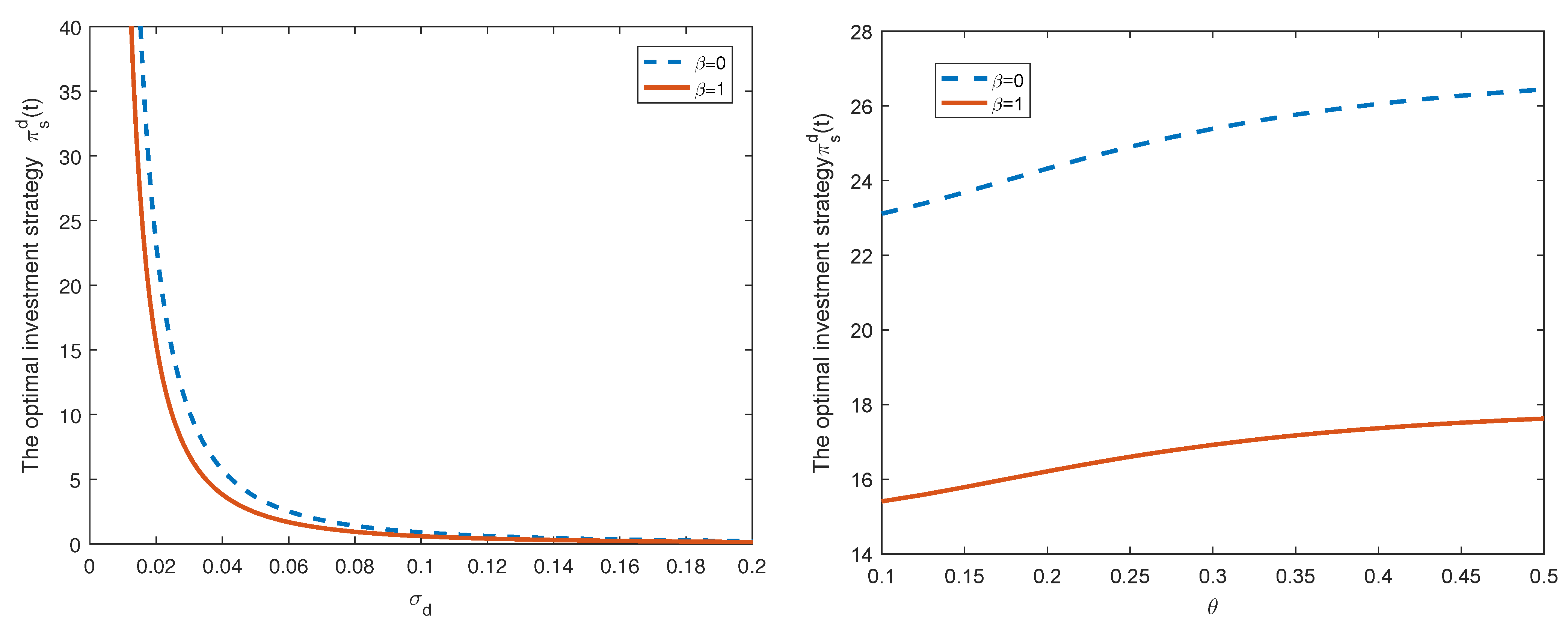
Figure 1 depicts the plots of the robust optimal investment strategies against the volatilities ${\sigma }_d$ and $\theta$. From the left panel of Figure 1, we can find that the value of bond B held in the optimal investment strategy, denoted by ${\pi }_s^d\left(t\right)$, becomes much less as the volatility ${\sigma }_d$ increases. The greater the volatility, the greater the risk of stock price. Hence, the investors will naturally reduce their investment in domestic stocks when ${\sigma }_{\mathrm{d}}$ increases. In addition, the right panel of Figure 1 describes the relationship between $\theta$ and ${\pi }_s^{\mathrm{d}}\left(t\right)$. We can observe that the optimal investment strategy ${\pi }_s^{\mathrm{d}}\left(t\right)$ is an increasing function with respect to the variable $\theta$. When the volatility of the exchange rate risk increases, the foreign stock price risk will also increase; thus, the investors will reduce investment in foreign stocks and increase investment in domestic stocks. Finally, we also compare the optimal investment strategy in the ambiguity averse case with the corresponding strategy in the ambiguity neutral case. In Figure 1, $\beta =1$ denotes ambiguity aversion, and $\beta =0$ means ambiguity neutral. We can see that the value of the optimal investment strategy ${\pi }_s^{\mathrm{d}}\left(t\right)$ at $\beta =0$ is greater than the value at $\beta =1$. This verifies that the investors with ambiguity aversion will invest less in risky assets compared with those who are ambiguity neutral. The reason is that investors with ambiguity aversion are more risk averse, which brings less money to the risky assets.

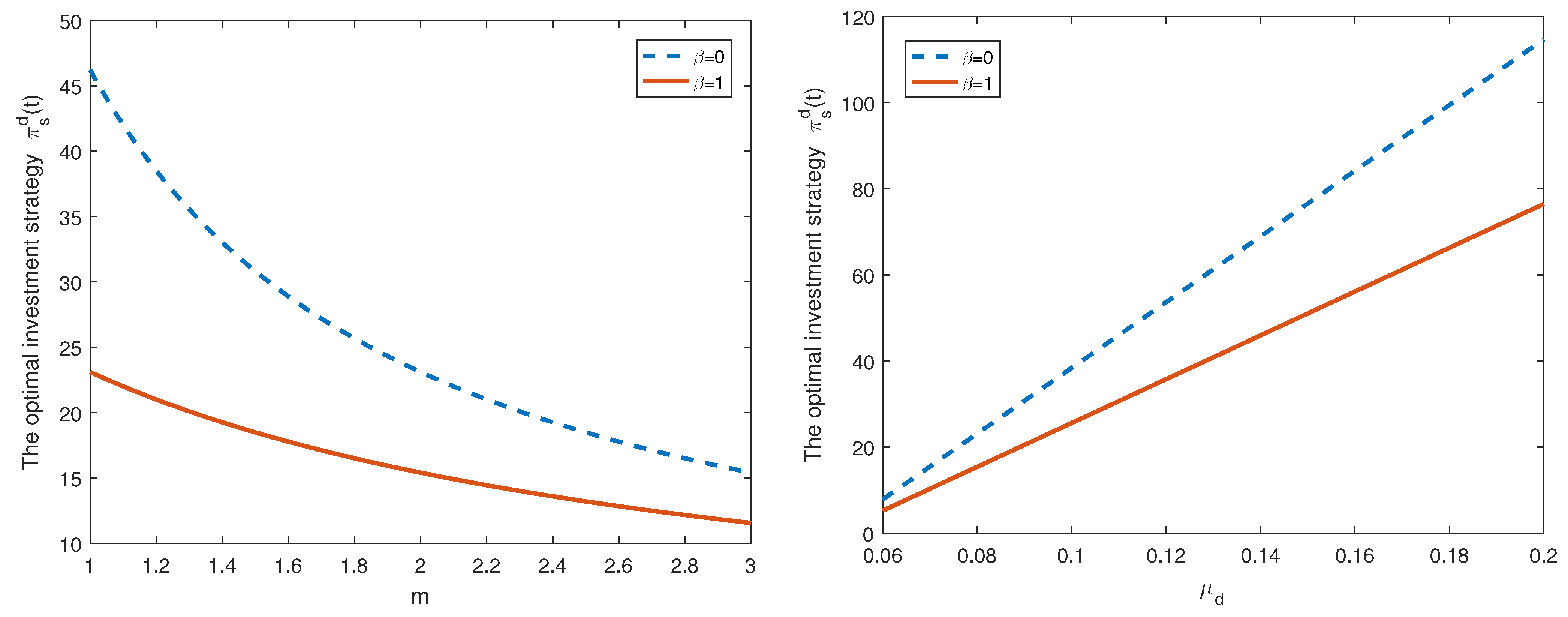
Figure 2 shows how the optimal investment strategy ${\pi }_s^{\mathrm{d}}\left(t\right)$ adjusts in response to the change of m and ${\mu }_d$. In Figure 2, m is a risk aversion coefficient; it measures the level of investor’s aversion to risk. As shown in the left panel of Figure 2, the optimal investment strategy ${\pi }_s^{\mathrm{d}}\left(t\right)$ decreases as the risk aversion coefficient m increases. This is because the investors will reduce their investment amount of the risky asset when the investors with a lower risk aversion parameter detest risk more. ${\mu }_d$ is the appreciate rate of the stock $S^d$. Since a high appreciate rate ${\mu }_d$ leads to a high yield, we think that there is a positive relationship between ${\mu }_d$ and ${\pi }_s^d\left(t\right)$. Indeed, it can be seen from the right panel of Figure 3 that ${\pi }_s^d\left(t\right)$ increases as ${\mu }_d$ increases. Hence, this result is also consistent with our conjecture.

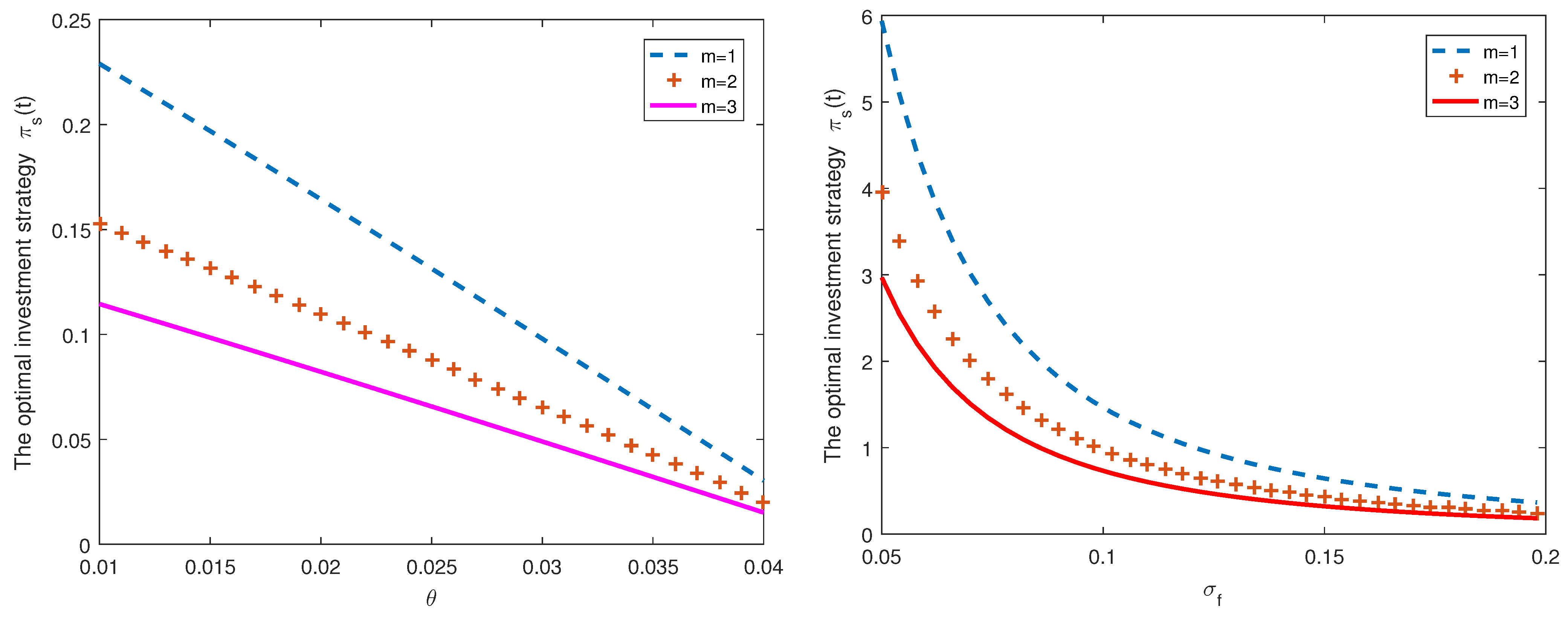
Figure 3 presents the influence of different $\theta$, m and ${\sigma }_f$ values on the optimal investment strategy ${\pi }_s\left(t\right)$. We observe that the negative correlation between $\theta$ and the optimal investment strategy ${\pi }_s\left(t\right)$ from the left panel of Figure 3. The cause for such results is very obvious, the larger $\theta$ means the greater volatility of exchange rate risk. The increased volatility of exchange rate risk may lead to investment losses; then, the investors will reduce the investment amount in the foreign stocks. Compared with Figure 2, we conclude that the impact of m on the optimal investment strategy ${\pi }_s\left(t\right)$ is the same as the influence of the optimal investment strategy ${\pi }_s^{\mathrm{d}}\left(t\right)$. Moreover, we can also find that there is a negative relationship between ${\sigma }_{\mathrm{f}}$ and the optimal investment strategy ${\pi }_s\left(t\right)$. It implies that the volatility risk has a significant impact on the number of risky assets held in the optimal investment strategy ${\pi }_s\left(t\right)$.

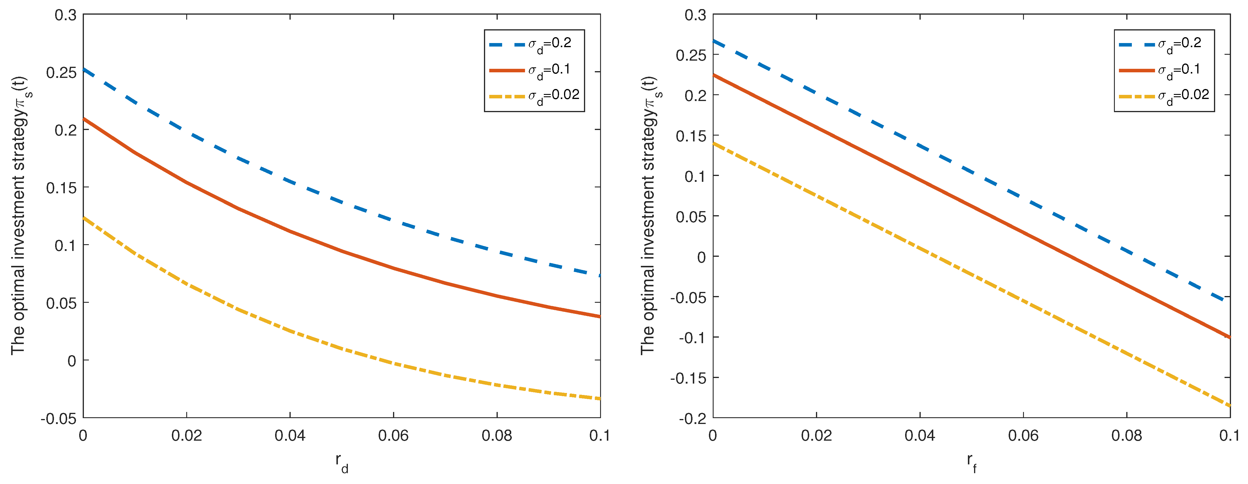
From Figure 4, we find that the increase of both domestic and foreign risk-free interest rates will reduce the amount of investment in the risky assets. This is because the investors will buy more risk-free assets but less risky assets when the risk-free interest rate increases. Compared with Figure 3, we can find that the investors will reduce their investment in foreign risky assets when the volatility of foreign risky assets increases, and the investors will choose to buy more foreign risky assets when the volatility of domestic risky assets increases. The reason is also obvious. When the volatility of domestic risky assets increases, the domestic risky assets will have a greater market price risk, and the investors will transfer part of their investment to foreign risky assets.

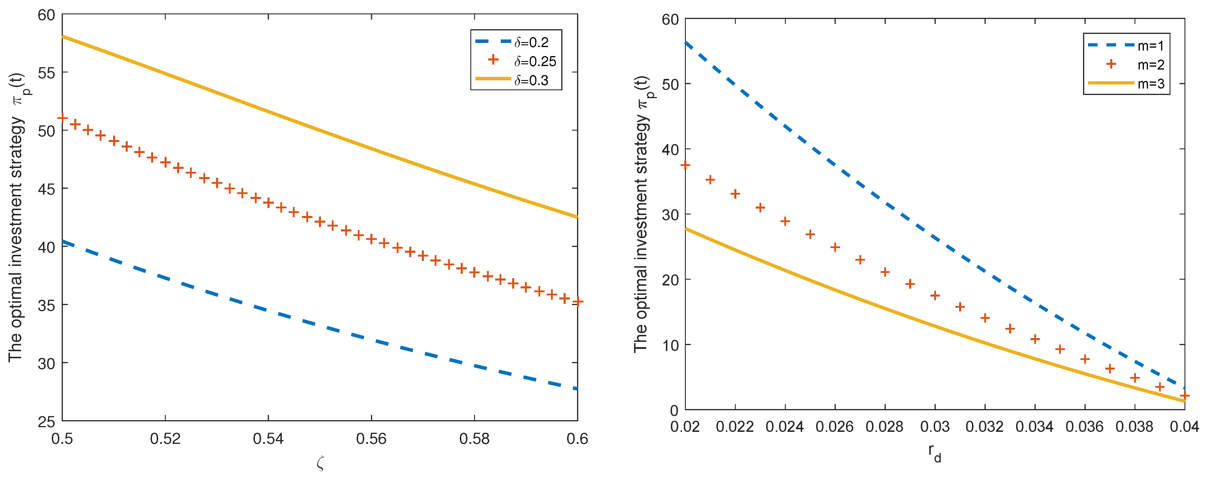
In Figure 5, we study the effect of model parameters $\delta$, $\zeta$, $r_d$ and m on the optimal investment strategy ${\pi }_p\left(t\right)$ in the blue-default case. From the left panel of Figure 5, we find that the number of defaultable bonds held in the optimal investment strategy will decrease as the loss rate $\zeta$ increases. It is obvious that a higher loss rate will lead to more potential loss. In order to minimize the investment risk, it is reasonable to reduce the holding positions in defaultable bonds. Furthermore, we also observe that there is a positive relationship between ${\pi }_p\left(t\right)$ and $\delta$. Our explanation is as follows: $\delta =\zeta h^Q$ is the default risk spread under the probability measure $Q^{\varphi }$, where $h^Q$ is the default intensity. A higher default intensity will lead to a higher yield before the default occurs; thus, the investors prefer to purchase more defaultable bonds as the default intensity $h^Q$ increases. Hence, ${\pi }_p\left(t\right)$ is an increase function with respect to $\delta$ when $\zeta$ is fixed. The right panel of Figure 5 plots the graph of the optimal trading strategy ${\pi }_p\left(t\right)$ invested in defaultable bonds as a function of the risk-free interest rate $r_d$. We observe that the optimal investment strategy is decreasing with respect to the risk-free interest rate $r_d$; it means that the investors should reduce the defaultable bond investment when the risk-free interest rate $r_d$ is increasing. This behavior of the optimal investment strategy is consistent with economic intuition. Moreover, we also present the numerical results of the optimal trading strategy ${\pi }_p\left(t\right)$ by varying the risk aversion coefficient m. We can find that the optimal trading strategy ${\pi }_p\left(t\right)$ is a decreasing function with respect to the risk aversion coefficient m. This may be interpreted as follows: When m is increasing, i.e., the investors are more risk-averse, they will reduce the investment in defaultable bonds.

5. Conclusions

This article focuses on an optimal investment problem with exchange rate risk and default risk when the investors are ambiguity averse. The price dynamics of exchange rate and domestic and foreign stocks are modeled by the Geometric Brownian motions, and meanwhile, the defaultable price process follows a jump process. To obtain the explicit expression of optimal investment strategy, an optimal portfolio problem framework with ambiguity aversion is first set up by using the robust control method. Second, the optimal investment problem is transformed to the corresponding HJB equation by the dynamic principle. Due to the existence of default risk, the HJB equation is usually too complicated to solve. Hence, we divide the HJB equation into the pre-default case and the post-default case. Finally, we derive the analytical solutions of the optimal investment strategies and the value functions by solving two HJB equations with the first order optimal condition. We find that the model uncertainty has a significant effect on the optimal investment strategies, and the investors with ambiguity aversion prefer to invest less risky assets than that of the investors who are ambiguity neutral. Moreover, we illustrate that if the volatility of the exchange rate risk increases, the investors will reduce their investment in foreign risky assets and meanwhile increase investment in domestic risky assets. This implies that an international investor must not ignore the exchange rate risk. In particular, our results also show that the optimal investment strategies are affected by the intensity of the default risk spread in the pre-default case.

The method in our work can also be used to solve other optimal investment portfolio problems involving default risk and exchange risk and model uncertainty. This article assumes that the price dynamics of the stocks and exchange rate follows the geometric Brownian motion. However, the implied volatility curve looks like a “smile”, not a constant. In the future research, we will incorporate the stochastic volatility into the stocks and exchange rate price dynamics to capture the volatility smile phenomena. Furthermore, this article shows that ambiguity aversion, exchange rate risk and default risk have a significant effect on the optimal investment strategies by some numerical results. It is challenging but necessary to analyze the impact of these factors on the optimal investment strategy through empirical analysis in future research.