Construction of Column-Orthogonal Designs with Two-Dimensional Stratifications

Abstract

For the design of computer experiments, column orthogonality and space-filling are two desirable properties. In this paper, we develop methods for constructing a new class of column-orthogonal designs (ODs) with two-dimensional stratifications on finer grids, including orthogonal Latin hypercube designs (OLHDs) as special cases. In addition to being column-orthogonal, these designs have good space-filling properties in two dimensions. The resulting designs achieve stratifications on $s^2\times s$ or $s\times s^2$ grids, and most column pairs satisfy stratifications on $s^2\times s^2$ grids. Moreover, many column pairs can achieve stratifications on $s^4\times s^2$ and $s^2\times s^4$ grids. Furthermore, the obtained space-filling ODs can have $s^6$ levels, $s^4$ levels, and mixed levels, as required for different needs.

1. Introduction

Computer experiments have been widely used recently to explore complex systems in many fields; space-filling and column orthogonality are desirable properties in the design of computer experiments [1]. The space-filling property, which measures the uniformity of the design points in the experimental region, is a fundamental criterion for evaluating designs for computer experiments. Latin hypercube designs (LHDs), proposed by [2], are widely used space-filling designs for computer experiments. An LHD with n runs and m factors, denoted as LHD$(n,m)$, is an $n\times m$ matrix with each column a permutation of n equally spaced levels. Such a design achieves the maximum stratification in each dimension. Based on the effect sparsity principle [3], for a high-dimensional design region, only a handful of the factors are expected to be active. In [4], the author proposed orthogonal array (OA)-based LHDs which improve the low-dimensional projection properties of random LHDs. In [5,6], the authors discussed space-filling designs with good projection properties in low dimensions. Recently, ref. [7] introduced strong orthogonal arrays, and [8] proposed mappable nearly orthogonal arrays. Both of these two kinds of arrays have better space-filling properties than ordinary orthogonal arrays.

Column orthogonality is a desirable property for LHDs; when a linear model is fitted, this property ensures that the estimates of the main effects are uncorrelated. In addition, orthogonality can be viewed as a stepping stone to space-filling designs when Gaussian process models are considered [9]. There are many ways to construct orthogonal LHDs (OLHDs); see, e.g., [10,11,12,13,14,15] and the references therein. Among them, the method of rotation has attracted widespread attention. In the extant literature, few works have simultaneously considered both the space-filling property and column orthogonality. In [16], the authors constructed OLHDs which achieved stratifications on $s^2\times s$ or $s\times s^2$ grids, with most column pairs achieving stratifications on $s^2\times s^2$ grids. In [17], the authors provided column-orthogonal designs (ODs) with two-dimensional stratifications. In [18], the authors studied ODs with two-dimensional and three-dimensional stratifications, while [15] proposed ODs with multi-dimensional stratifications.

The goal of the present paper is to construct ODs with stratifications on finer grids, i.e., $s^2\times s^2$, $s^4\times s^2$, and $s^2\times s^4$. We first introduce a new class of OLHDs with $s^{d+2k}$ runs by rotating s-level OAs, where $d+2k$ can be any positive even integer not smaller than 4 and $d=2^c$ $(c\ge 2)$. We additionally introduce a new class of ODs with flexible run sizes. All these designs guarantee desirable two-dimensional space-filling properties. Most column pairs of the resulting designs can achieve stratifications on $s^2\times s^2$ grids. Moreover, many column pairs can satisfy stratifications on $s^4\times s^2$ and $s^2\times s^4$ grids. Furthermore, the resulting ODs can have $s^6$ or $s^4$ levels and mixed levels.

The rest of this paper is organized as follows: Section 2 introduces preliminaries used in this paper; Section 3 proposes the general construction method for OLHDs and extends it to accommodate more factors; Section 4 concentrates on the construction of ODs with $s^6$ levels, $s^4$ levels, and mixed levels; finally, concluding remarks are provided in Section 5. All proofs are deferred to Appendix A.

2. Definitions and Notation

We use $D(n,s_1,\dots ,s_m)$ to denote a balanced design of n runs and m factors, with each of the $s_j$ levels from $\{0,1,\dots ,s_j-1\}$. When all the instances of $s_j$ are equal to s, the design is a symmetric balanced design $D(n,s^m)$. Further, if $s=n$, it is an LHD, denoted as LHD$(n,m)$.

A mixed-level orthogonal array (OA) with strength t and levels $s_1,\dots ,s_m$, denoted as OA$(n,m,s_1\times \cdots \times s_m,t)$, satisfies the requirement that all possible level combinations for any columns t occur with the same frequency. When all $s_j$ are equal to s, the array is symmetric and denoted as OA$(n,m,s,t)$. For an OA$(n,m,s,t)$, it must have $n=\lambda s^t$ for some integer $\lambda$, which is the index of the OA.

For an array with n runs and m factors, we say it achieves a stratification on an $s_1\times \cdots \times s_p$ grid for some $p\ge 2$ if the corresponding p columns of it can be collapsed into an OA $(n,p,s_1\times \cdots \times s_p,p)$.

The correlation between two vectors $a={(a_1,\dots ,a_n)}^T$ and $b={(b_1,\dots ,b_n)}^T$ is defined as

$$\rho (a,b)=\frac{{\sum }_{i=1}^n(a_i-\overline{a})(b_i-\overline{b})}{\sqrt{{\sum }_{i=1}^n{(a_i-\overline{a})}^2{\sum }_{i=1}^n{(b_i-\overline{b})}^2}},$$

where $\overline{a}={\sum }_{i=1}^n{a}_i/n$ and $\overline{b}={\sum }_{i=1}^n{b}_i/n$. The average correlation of a design $D=(d_1,\dots ,d_m)$ is defined as

$${\rho }_{ave}\left(D\right)=\frac{{\sum }_{j\ne k}\rho (d_j,d_k)}{m(m-1)}.$$

Two vectors are said to be column-orthogonal if the correlation between them is 0. A design $D(n,s^m)$ is said to be column-orthogonal, denoted as OD$(n,s^m)$, if any two of its columns are column-orthogonal. Obviously, any OA$(n,m,s,t)$ with $t\ge 2$ is an OD$(n,s^m)$. Similarly, we have OLHD $(n,m)$.

To facilitate the study of orthogonality, we sometimes center the $s^2$ levels of an OD $(n,{\left(s^2\right)}^m)$ into

$$\Omega \left(s^2\right)=\{u-(s^2-1)/2|u=0,\dots ,s^2-1\}.$$

(1)

Let $GF\left(s^d\right)=\{a_0+a_{1}x+\cdots +a_{d-1}{x}^{d-1},a_0,\dots ,a_{d-1}\in GF\left(s\right)\}$ be a Galois field of order $s^d$ and let $GF\left(s\right)=\{0,\dots ,s-1\}$ be a Galois field of order s. We denote an $r\times c$ matrix with entries from $GF\left(s^2\right)=\{a_0+a_{1}x,a_0,a_1\in GF\left(s\right)\}$ as $D(r,c,s^2)$, which is called a difference scheme if it satisfies the requirement that, for any i and j with $1\le i\ne j\le c$, the vector difference of the ith and jth columns contains every element of $GF\left(s^2\right)$ equally often.

For two matrices $A={\left(a_{ij}\right)}_{m\times n}$ and $B={\left(b_{ij}\right)}_{u\times v}$ with entries from $GF\left(s^2\right)$, we define

$$A\oplus B=\left(\begin{array}{ccc}{a}_{11}+B& \cdots & a_{1n}+B\\ ⋮& & ⋮\\ a_{m1}+B& \cdots & a_{mn}+B\end{array}\right),$$

where + is the addition defined on $GF\left(s^2\right)$.

For any design A with entries from $\{0,1,\dots ,s^2-1\}$, let ${\Phi }_0\left(A\right)=A$; we define

$${\Phi }_k\left(A\right)=\left({\phi }_{k,1}\left(A\right),\dots ,{\phi }_{k,\lfloor s^2/2\rfloor }\left(A\right)\right)$$

(2)

for $k=1,2,\dots$, and define

$${\phi }_{k,j}\left(A\right)=\left(d_{2j-1}\oplus {\Phi }_{k-1}\left(A\right),d_{2j}\oplus {\Phi }_{k-1}\left(A\right)\right),$$

where $j=1,\dots ,\lfloor s^2/2\rfloor$, $\lfloor h\rfloor$ denotes the largest integer less than or equal to h and $d_l$ denotes the lth column in the difference scheme $D(s^2,s^2,s^2)=(d_1,\dots ,d_{s^2})$ for $l=1,\dots ,s^2$.

Let

$$R_{1,0}=\left(\begin{array}{cc}{s}^2& -1\\ 1& s^2\end{array}\right),R_{u,0}=\left(\begin{array}{cc}{s}^{2^u}{R}_{u-1,0}& -R_{u-1,0}\\ R_{u-1,0}& s^{2^u}{R}_{u-1,0}\end{array}\right)(u\ge 2),$$

$$Q_1=\left(\begin{array}{cc}1& 0\\ 0& -1\end{array}\right),\mathrm{and}{Q}_u=\left(\begin{array}{cc}{Q}_{u-1}& 0\\ 0& -Q_{u-1}\end{array}\right)(u\ge 2).$$

Then, we define

$$R_{u,1}=\left(\begin{array}{cc}{s}^2{R}_{u,0}& -Q_u\\ Q_u& s^2{R}_{u,0}\end{array}\right),R_{u,k}=\left(\begin{array}{cc}{s}^2{R}_{u,k-1}& -Q_{u+k-1}\\ Q_{u+k-1}& s^2{R}_{u,k-1}\end{array}\right)(u\ge 2,k\ge 2).$$

(3)

For a prime power $s^2$, let $C=(c_1,\dots ,c_m)$ be an OA$(n,m,s^2,2)$ with entries from $GF\left(s^2\right)$ and let D be a difference scheme $D(s^2,s^2,s^2)=(d_1,\dots ,d_{s^2})$. We now create

$$E_i=D\oplus c_i=(d_1\oplus c_i,\dots ,d_{s^2}\oplus c_i),$$

(4)

for $i=1,\dots ,m$ and define

$$E=(E_1,\dots ,E_m).$$

(5)

For a prime s and integer d with $d=2^c$ and $c\ge 2$, we denote the d columns of an $s^d$-run full factorial design as $\mathbf{1},\dots ,\mathbf{d}$. Any generated column including each column of $\mathbf{1},\dots ,\mathbf{d}$ can be denoted as ${\mathbf{1}}^{a_0}\dots {\mathbf{d}}^{a_{d-1}}$ for some $a_0,\dots ,a_{d-1}\in GF\left(s\right)$, and corresponds to a nonzero element $a_0+a_{1}x+\cdots +a_{d-1}{x}^{d-1}$ in $GF\left(s^d\right)$. Here, let $p=\lfloor (s^d-1)/\left(d(s-1)\right)\rfloor$.

As discussed in [11], the corresponding columns of the first $pd$ non-zero elements of $GF\left(s^d\right)$, $x^0,x^1,\dots ,x^{pd-1}$ modulo $f\left(x\right)$ form a regular design D, where $f\left(x\right)$ is a primitive polynomial of order d. Any d consecutive columns of D form a full factorial design, denoted as $B_1,B_2,\dots ,B_p$ and $B_i=(x^{(i-1)d},x^{(i-1)d+1},\dots ,x^{id-1})$ mod $f\left(x\right)$, $i=1,\dots ,p$. Let $B_i=(b_{i,1},\dots ,b_{i,d})$, defining $f_{i,j}=s{b}_{i,2j-1}+b_{i,2j}$ for $i=1,\dots ,p$, $j=1,\dots ,d/2$. Then, we have

$$F_i=(f_{i,1},\dots ,f_{i,d/2})$$

(6)

and

$$F=(F_1,\dots ,F_p).$$

(7)

Without particular explanation, in this paper, s is a prime, $k\ge 0$, d is an integer with $d=2^c$, $c\ge 2$, and $p=\lfloor (s^d-1)/\left(d(s-1)\right)\rfloor$. We provide an illustrative example in the following.

Example 1. 

For $s=3$ and $d=4$, we denote the $3^4$ full factorial design as $(\mathbf{1},\mathbf{2},\mathbf{3},\mathbf{4})$. Here, $GF\left(3^4\right)=\{a_0+a_{1}x+a_2{x}^2+a_3{x}^3,a_0,a_1,a_2,a_3\in GF\left(3\right)\}$, with the primitive polynomial $f\left(x\right)=x^4+x+2$. Then, $x^0$, $x^1$, $x^2$, $x^3$ modulo $f\left(x\right)$ are 1, x, $x^2$, $x^3$, which correspond to columns $\mathbf{1}$, $\mathbf{2}$, $\mathbf{3}$, $\mathbf{4}$. Similarly, we have the elements of $x^4,x^5,\dots ,x^{39}$ modulo $f\left(x\right)$. For example, ${\mathbf{12}}^{\mathbf{2}}$ is obtained by $x^4$ modulo $f\left(x\right)$. The obtained full factorial designs $B_1,\dots ,B_{10}$ are shown in

Table 1. The obtained $3^4$ full factorial designs.

	${\mathit{b}}_{\mathit{i}1}$	${\mathit{b}}_{\mathit{i}2}$	${\mathit{b}}_{\mathit{i}3}$	${\mathit{b}}_{\mathit{i}4}$
$B_1$	$\mathbf{1}\left(x^0\right)$	$\mathbf{2}\left(x^1\right)$	$\mathbf{3}\left(x^2\right)$	$\mathbf{4}\left(x^3\right)$
$B_2$	${\mathbf{12}}^{\mathbf{2}}\left(x^4\right)$	${\mathbf{23}}^{\mathbf{2}}\left(x^5\right)$	${\mathbf{34}}^{\mathbf{2}}\left(x^6\right)$	${\mathbf{12}}^{\mathbf{2}}{\mathbf{4}}^{\mathbf{2}}\left(x^7\right)$
$B_3$	$\mathbf{123}\left(x^8\right)$	$\mathbf{234}\left(x^9\right)$	${\mathbf{12}}^{\mathbf{2}}\mathbf{34}\left(x^{10}\right)$	${\mathbf{123}}^{\mathbf{2}}\mathbf{4}\left(x^{11}\right)$
$B_4$	${\mathbf{14}}^{\mathbf{2}}\left(x^{12}\right)$	$\mathbf{12}\left(x^{13}\right)$	$\mathbf{23}\left(x^{14}\right)$	$\mathbf{34}\left(x^{15}\right)$
$B_5$	${\mathbf{12}}^{\mathbf{2}}\mathbf{4}\left(x^{16}\right)$	${\mathbf{13}}^{\mathbf{2}}\left(x^{17}\right)$	${\mathbf{24}}^{\mathbf{2}}\left(x^{18}\right)$	${\mathbf{12}}^{\mathbf{2}}{\mathbf{3}}^{\mathbf{2}}\left(x^{19}\right)$
$B_6$	${\mathbf{23}}^{\mathbf{2}}{\mathbf{4}}^{\mathbf{2}}\left(x^{20}\right)$	${\mathbf{12}}^{\mathbf{2}}{\mathbf{3}}^{\mathbf{2}}\mathbf{4}\left(x^{21}\right)$	${\mathbf{13}}^{\mathbf{2}}{\mathbf{4}}^{\mathbf{2}}\left(x^{22}\right)$	$\mathbf{124}\left(x^{23}\right)$
$B_7$	$\mathbf{13}\left(x^{24}\right)$	$\mathbf{24}\left(x^{25}\right)$	${\mathbf{12}}^{\mathbf{2}}\mathbf{3}\left(x^{26}\right)$	${\mathbf{23}}^{\mathbf{2}}\mathbf{4}\left(x^{27}\right)$
$B_8$	${\mathbf{12}}^{\mathbf{2}}{\mathbf{34}}^{\mathbf{2}}\left(x^{28}\right)$	${\mathbf{1234}}^{\mathbf{2}}\left(x^{29}\right)$	${\mathbf{13}}^{\mathbf{2}}{\mathbf{4}}^{\mathbf{2}}\left(x^{30}\right)$	${\mathbf{123}}^{\mathbf{2}}\mathbf{4}\left(x^{31}\right)$
$B_9$	${\mathbf{134}}^{\mathbf{2}}\left(x^{32}\right)$	${\mathbf{124}}^{\mathbf{2}}\left(x^{33}\right)$	${\mathbf{123}}^{\mathbf{2}}\left(x^{34}\right)$	${\mathbf{234}}^{\mathbf{2}}\left(x^{35}\right)$
$B_{10}$	${\mathbf{12}}^{\mathbf{2}}{\mathbf{3}}^{\mathbf{2}}{\mathbf{4}}^{\mathbf{2}}\left(x^{36}\right)$	$\mathbf{1234}\left(x^{37}\right)$	$\mathbf{134}\left(x^{38}\right)$	$\mathbf{14}\left(x^{39}\right)$

, where $b_{ij}$ is the jth column in $B_i$ for $i=1,\dots ,10$ and $j=1,\dots ,4$.

3. Construction of Orthogonal LHDs

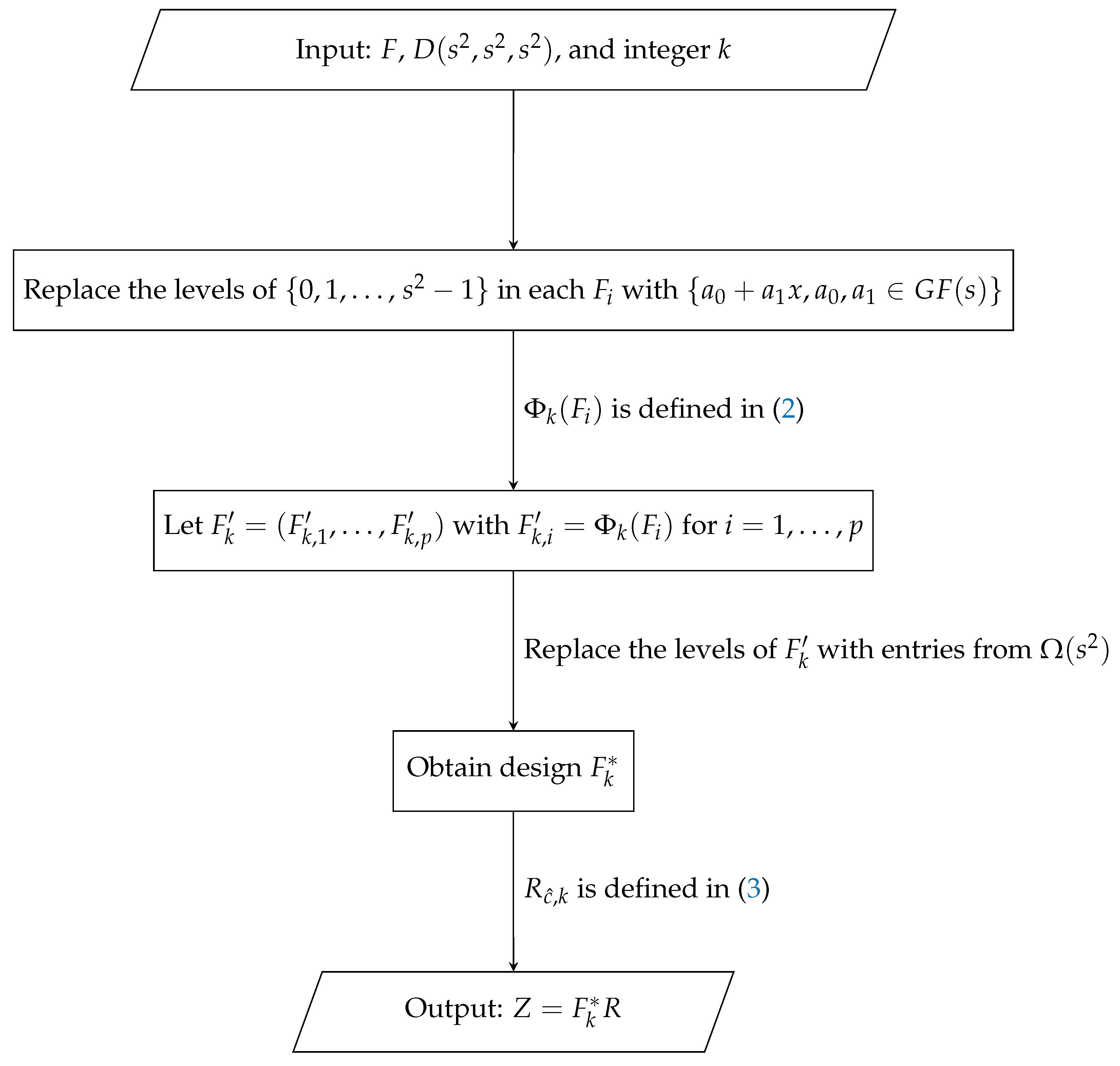
This section first introduces a rotation method in Algorithm 1 to construct OLHDs with attractive stratification properties, then generalizes the method to enlarge the columns of these LHDs.

To make it easier for readers to understand the algorithm, we provide the flowchart in Figure 1 to explain the algorithm.

To measure the stratification properties of a design with m columns, we define the following two proportions:

$${\pi }_{\alpha }=\frac{r_{\alpha }}{\left(\genfrac{}{}{0pt}{}{m}{2}\right)},{\pi }_{\beta }=\frac{r_{\beta }}{\left(\genfrac{}{}{0pt}{}{m}{2}\right)},$$

where $r_{\alpha }$ is the number of column pairs that achieve stratifications on $s^2\times s^2$ grids and $r_{\beta }$ is the number of column pairs that achieve stratifications on $s^4\times s^2$ and $s^2\times s^4$ grids. The properties of the designs in Algorithm 1 are summarized in Theorem 1.

Algorithm 1 Construction of OLHDs

Input:  $F=(F_1,\dots ,F_p)$, $D(s^2,s^2,s^2)=(d_1,\dots ,d_{s^2})$, and integer k.  1:  Let $F=(F_1,\dots ,F_p)$ as defined in (6) and replace the levels of $\{0,1,\dots ,$ $s^2-1\}$ in each $F_i$ with $\{a_0+a_{1}x,a_0,a_1\in GF\left(s\right)\}$.  2:  Obtain a difference scheme $D(s^2,s^2,s^2)=(d_1,\dots ,d_{s^2})$. For a given k, let $F_k^{\prime }=(F_{k,1}^{\prime },\dots ,F_{k,p}^{\prime })$ with $F_{k,i}^{\prime }={\Phi }_k\left(F_i\right)$ for $i=1,\dots ,p$, where ${\Phi }_k\left(F_i\right)$ is defined in (2).  3:  Replace the levels of $F_k^{\prime }$ with entries from $\Omega \left(s^2\right)$ as in (1) and denote the resulting design as $F_k^{*}$.  4:  Obtain $Z=F_k^{*}R$, where $R={\mathbf{I}}_{p\lfloor s^2/2\rfloor }\otimes R_{\widehat{c},k}$, $\widehat{c}={log}_{2}d-1$, and $R_{\widehat{c},k}$ is defined in (3). Output:  Design Z.

Theorem 1. 

Design Z in Algorithm 1 is an OLHD$(s^{d+2k},m)$ where $m=pd\gamma /2$ and $\gamma ={\lfloor s^2/2\rfloor }^k{2}^k$, and has the following properties:

(1)

Any two columns achieve a stratification on an $s^2\times s$ or $s\times s^2$ grid;

(2)

The proportion of column pairs achieving stratifications on $s^2\times s^2$ grids satisfies ${\pi }_{\alpha }\ge 1-2(s-1)/(m-1)$;

(3)

The proportion of column pairs achieving stratifications on $s^2\times s^4$ and $s^4\times s^2$ grids satisfies ${\pi }_{\beta }\ge 1-(m/\gamma +2\gamma s-\gamma -2s)/(m-1)$.

For this, we use the following illustrative example.

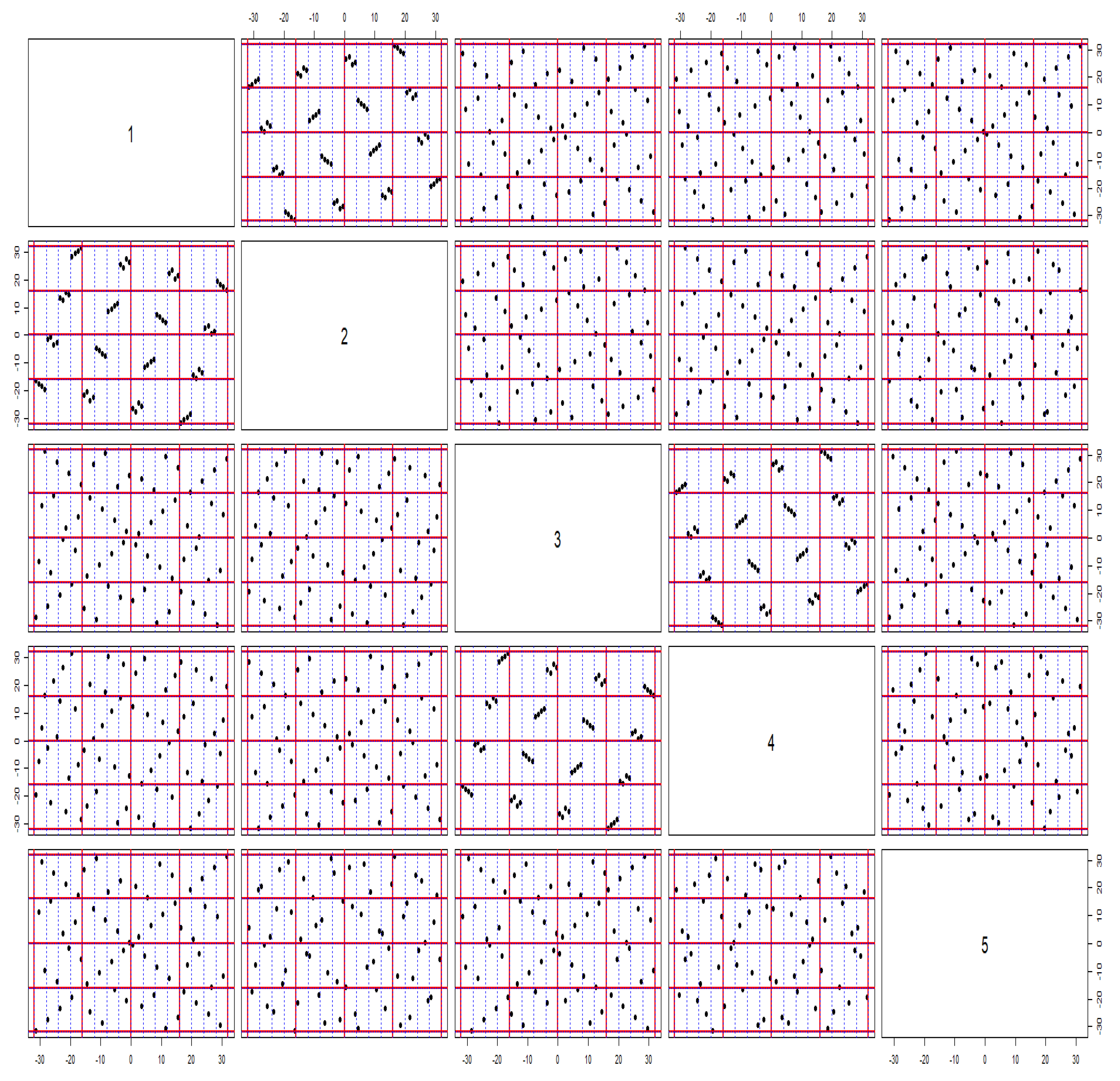
Example 2. 

For $s=2$ and $d=4$, we denote the four independent columns as $\mathbf{1}$, $\mathbf{2}$, $\mathbf{3}$, $\mathbf{4}$, while the generated columns of these four columns are denoted as $\mathbf{12}$, $\mathbf{13}$, $\mathbf{14}$, $\mathbf{23}$, $\mathbf{24}$, $\mathbf{34}$, $\mathbf{123}$, $\mathbf{124}$, $\mathbf{134}$, $\mathbf{234}$, $\mathbf{1234}$. We have $GF\left(2^4\right)=\{a_0+a_{1}x+a_2{x}^2+a_3{x}^3,a_i\in$ $GF\left(2\right)\}$ with $GF\left(2\right)=\{0,1\}$ and the primitive polynomial $f\left(x\right)=x^4+x+1$. It is easy to obtain three full factorial designs $B_1=(\mathbf{1},\mathbf{2},\mathbf{3},\mathbf{4})$, $B_2=(\mathbf{12},\mathbf{23},\mathbf{34},\mathbf{124})$, and $B_3=(\mathbf{13},\mathbf{24},\mathbf{123},\mathbf{234})$. Then, we have $F_1=(2\times \mathbf{1}+\mathbf{2},2\times \mathbf{3}+\mathbf{4})$, $F_2=(2\times \mathbf{12}+\mathbf{23},2\times \mathbf{34}+\mathbf{124})$, and $F_3=(2\times \mathbf{13}+\mathbf{24},2\times \mathbf{123}+\mathbf{234})$. Thus, $F=(F_1,F_2,F_3)$, which is displayed in

Table 2. F in Example 2.

${\mathit{F}}_1$		${\mathit{F}}_2$		${\mathit{F}}_3$
$2\times \mathbf{1}+\mathbf{2}$	$2\times \mathbf{3}+\mathbf{4}$	$2\times \mathbf{12}+\mathbf{23}$	$2\times \mathbf{34}+\mathbf{124}$	$2\times \mathbf{13}+\mathbf{24}$	$2\times \mathbf{123}+\mathbf{234}$
0	0	0	0	0	0
0	1	0	$x+1$	1	1
0	x	1	x	x	$x+1$
0	$x+1$	1	1	$x+1$	x
1	0	$x+1$	1	1	$x+1$
1	1	$x+1$	x	0	x
1	x	x	$x+1$	$x+1$	1
1	$x+1$	x	0	x	0
x	0	x	1	x	1
x	1	x	x	$x+1$	x
x	x	$x+1$	$x+1$	0	$x+1$
x	$x+1$	$x+1$	0	1	0
$x+1$	0	1	0	$x+1$	1
$x+1$	1	1	$x+1$	x	0
$x+1$	x	0	x	1	x
$x+1$	$x+1$	0	1	0	$x+1$

.

In this way, we obtain a difference scheme $D(4,4,4)=(d_1,d_2,d_3,$ $d_4)$, denoted as

$$D=\left(\begin{array}{cccc}0& 0& 0& 0\\ 0& 1& x& x+1\\ 0& x& x+1& 1\\ 0& x+1& 1& x\end{array}\right),$$

with $F_1^{\prime }=(F_{1,1}^{\prime },F_{1,2}^{\prime },F_{1,3}^{\prime })$, where $F_{1,i}^{\prime }={\Phi }_1\left(F_i\right)=(d_0\oplus F_i,d_1\oplus F_i,d_2\oplus F_i,d_3\oplus F_i)$ for $i=1,2,3$. We can obtain $F_1^{*}$ by replacing the levels of $F_1^{\prime }$ with entries from $\{-1.5,-0.5,0.5,1.5\}$. Then, we rotate $F_1^{*}$ by $R=I_6\otimes R_{1,1}$ to generate an OLHD$(64,24)$, where

$$R_{1,1}=\left(\begin{array}{cccc}16& -4& -1& 0\\ 4& 16& 0& 1\\ 1& 0& 16& -4\\ 0& -1& 4& 16\end{array}\right).$$

The resulting OLHD$(64,24)$ is displayed in

Table A1. The OLHD$(64,24)$ used in Example 2.

	1	2	3	4	5	6	7	8	9	10	11	12	13	14	15	16	17	18	19	20	21	22	23	24
1	−31.5	−16.5	−28.5	−19.5	−31.5	−16.5	−28.5	−19.5	−31.5	−16.5	−28.5	−19.5	−31.5	−16.5	−28.5	−19.5	−31.5	−16.5	−28.5	−19.5	−31.5	−16.5	−28.5	−19.5
2	−27.5	−1.5	−24.5	−2.5	−27.5	−1.5	−24.5	−2.5	−19.5	28.5	−16.5	31.5	−19.5	28.5	−16.5	31.5	−10.5	−5.5	−9.5	−6.5	−10.5	−5.5	−9.5	−6.5
3	−23.5	13.5	−20.5	14.5	−23.5	13.5	−20.5	14.5	−6.5	9.5	−5.5	10.5	−6.5	9.5	−5.5	10.5	14.5	20.5	13.5	23.5	14.5	20.5	13.5	23.5
4	−19.5	28.5	−16.5	31.5	−19.5	28.5	−16.5	31.5	−10.5	−5.5	−9.5	−6.5	−10.5	−5.5	−9.5	−6.5	27.5	1.5	24.5	2.5	27.5	1.5	24.5	2.5
5	−14.5	−20.5	−13.5	−23.5	−14.5	−20.5	−13.5	−23.5	23.5	−13.5	20.5	−14.5	23.5	−13.5	20.5	−14.5	−2.5	24.5	−1.5	27.5	−2.5	24.5	−1.5	27.5
6	−10.5	−5.5	−9.5	−6.5	−10.5	−5.5	−9.5	−6.5	27.5	1.5	24.5	2.5	27.5	1.5	24.5	2.5	−23.5	13.5	−20.5	14.5	−23.5	13.5	−20.5	14.5
7	−6.5	9.5	−5.5	10.5	−6.5	9.5	−5.5	10.5	14.5	20.5	13.5	23.5	14.5	20.5	13.5	23.5	19.5	−28.5	16.5	−31.5	19.5	−28.5	16.5	−31.5
8	−2.5	24.5	−1.5	27.5	−2.5	24.5	−1.5	27.5	2.5	−24.5	1.5	−27.5	2.5	−24.5	1.5	−27.5	6.5	−9.5	5.5	−10.5	6.5	−9.5	5.5	−10.5
9	2.5	−24.5	1.5	−27.5	2.5	−24.5	1.5	−27.5	6.5	−9.5	5.5	−10.5	6.5	−9.5	5.5	−10.5	10.5	5.5	9.5	6.5	10.5	5.5	9.5	6.5
10	6.5	−9.5	5.5	−10.5	6.5	−9.5	5.5	−10.5	10.5	5.5	9.5	6.5	10.5	5.5	9.5	6.5	31.5	16.5	28.5	19.5	31.5	16.5	28.5	19.5
11	10.5	5.5	9.5	6.5	10.5	5.5	9.5	6.5	31.5	16.5	28.5	19.5	31.5	16.5	28.5	19.5	−27.5	−1.5	−24.5	−2.5	−27.5	−1.5	−24.5	−2.5
12	14.5	20.5	13.5	23.5	14.5	20.5	13.5	23.5	19.5	−28.5	16.5	−31.5	19.5	−28.5	16.5	−31.5	−14.5	−20.5	−13.5	−23.5	−14.5	−20.5	−13.5	−23.5
13	19.5	−28.5	16.5	−31.5	19.5	−28.5	16.5	−31.5	−14.5	−20.5	−13.5	−23.5	−14.5	−20.5	−13.5	−23.5	23.5	−13.5	20.5	−14.5	23.5	−13.5	20.5	−14.5
14	23.5	−13.5	20.5	−14.5	23.5	−13.5	20.5	−14.5	−2.5	24.5	−1.5	27.5	−2.5	24.5	−1.5	27.5	2.5	−24.5	1.5	−27.5	2.5	−24.5	1.5	−27.5
15	27.5	1.5	24.5	2.5	27.5	1.5	24.5	2.5	−23.5	13.5	−20.5	14.5	−23.5	13.5	−20.5	14.5	−6.5	9.5	−5.5	10.5	−6.5	9.5	−5.5	10.5
16	31.5	16.5	28.5	19.5	31.5	16.5	28.5	19.5	−27.5	−1.5	−24.5	−2.5	−27.5	−1.5	−24.5	−2.5	−19.5	28.5	−16.5	31.5	−19.5	28.5	−16.5	31.5
17	−30.5	−17.5	−8.5	−7.5	11.5	4.5	29.5	18.5	−30.5	−17.5	−8.5	−7.5	11.5	4.5	29.5	18.5	−30.5	−17.5	−8.5	−7.5	11.5	4.5	29.5	18.5
18	−26.5	−0.5	−12.5	−22.5	15.5	21.5	25.5	3.5	−18.5	29.5	−4.5	11.5	7.5	−8.5	17.5	−30.5	−11.5	−4.5	−29.5	−18.5	30.5	17.5	8.5	7.5
19	−22.5	12.5	−0.5	26.5	3.5	−25.5	21.5	−15.5	−7.5	8.5	−17.5	30.5	18.5	−29.5	4.5	−11.5	15.5	21.5	25.5	3.5	−26.5	−0.5	−12.5	−22.5
20	−18.5	29.5	−4.5	11.5	7.5	−8.5	17.5	−30.5	−11.5	−4.5	−29.5	−18.5	30.5	17.5	8.5	7.5	26.5	0.5	12.5	22.5	−15.5	−21.5	−25.5	−3.5
21	−15.5	−21.5	−25.5	−3.5	26.5	0.5	12.5	22.5	22.5	−12.5	0.5	−26.5	−3.5	25.5	−21.5	15.5	−3.5	25.5	−21.5	15.5	22.5	−12.5	0.5	−26.5
22	−11.5	−4.5	−29.5	−18.5	30.5	17.5	8.5	7.5	26.5	0.5	12.5	22.5	−15.5	−21.5	−25.5	−3.5	−22.5	12.5	−0.5	26.5	3.5	−25.5	21.5	−15.5
23	−7.5	8.5	−17.5	30.5	18.5	−29.5	4.5	−11.5	15.5	21.5	25.5	3.5	−26.5	−0.5	−12.5	−22.5	18.5	−29.5	4.5	−11.5	−7.5	8.5	−17.5	30.5
24	−3.5	25.5	−21.5	15.5	22.5	−12.5	0.5	−26.5	3.5	−25.5	21.5	−15.5	−22.5	12.5	−0.5	26.5	7.5	−8.5	17.5	−30.5	−18.5	29.5	−4.5	11.5
25	3.5	−25.5	21.5	−15.5	−22.5	12.5	−0.5	26.5	7.5	−8.5	17.5	−30.5	−18.5	29.5	−4.5	11.5	11.5	4.5	29.5	18.5	−30.5	−17.5	−8.5	−7.5
26	7.5	−8.5	17.5	−30.5	−18.5	29.5	−4.5	11.5	11.5	4.5	29.5	18.5	−30.5	−17.5	−8.5	−7.5	30.5	17.5	8.5	7.5	−11.5	−4.5	−29.5	−18.5
27	11.5	4.5	29.5	18.5	−30.5	−17.5	−8.5	−7.5	30.5	17.5	8.5	7.5	−11.5	−4.5	−29.5	−18.5	−26.5	−0.5	−12.5	−22.5	15.5	21.5	25.5	3.5
28	15.5	21.5	25.5	3.5	−26.5	−0.5	−12.5	−22.5	18.5	−29.5	4.5	−11.5	−7.5	8.5	−17.5	30.5	−15.5	−21.5	−25.5	−3.5	26.5	0.5	12.5	22.5
29	18.5	−29.5	4.5	−11.5	−7.5	8.5	−17.5	30.5	−15.5	−21.5	−25.5	−3.5	26.5	0.5	12.5	22.5	22.5	−12.5	0.5	−26.5	−3.5	25.5	−21.5	15.5
30	22.5	−12.5	0.5	−26.5	−3.5	25.5	−21.5	15.5	−3.5	25.5	−21.5	15.5	22.5	−12.5	0.5	−26.5	3.5	−25.5	21.5	−15.5	−22.5	12.5	−0.5	26.5
31	26.5	0.5	12.5	22.5	−15.5	−21.5	−25.5	−3.5	−22.5	12.5	−0.5	26.5	3.5	−25.5	21.5	−15.5	−7.5	8.5	−17.5	30.5	18.5	−29.5	4.5	−11.5
32	30.5	17.5	8.5	7.5	−11.5	−4.5	−29.5	−18.5	−26.5	−0.5	−12.5	−22.5	15.5	21.5	25.5	3.5	−18.5	29.5	−4.5	11.5	7.5	−8.5	17.5	−30.5
33	−29.5	−18.5	11.5	4.5	29.5	18.5	−11.5	−4.5	−29.5	−18.5	11.5	4.5	29.5	18.5	−11.5	−4.5	−29.5	−18.5	11.5	4.5	29.5	18.5	−11.5	−4.5
34	−25.5	−3.5	15.5	21.5	25.5	3.5	−15.5	−21.5	−17.5	30.5	7.5	−8.5	17.5	−30.5	−7.5	8.5	−8.5	−7.5	30.5	17.5	8.5	7.5	−30.5	−17.5
35	−21.5	15.5	3.5	−25.5	21.5	−15.5	−3.5	25.5	−4.5	11.5	18.5	−29.5	4.5	−11.5	−18.5	29.5	12.5	22.5	−26.5	−0.5	−12.5	−22.5	26.5	0.5
36	−17.5	30.5	7.5	−8.5	17.5	−30.5	−7.5	8.5	−8.5	−7.5	30.5	17.5	8.5	7.5	−30.5	−17.5	25.5	3.5	−15.5	−21.5	−25.5	−3.5	15.5	21.5
37	−12.5	−22.5	26.5	0.5	12.5	22.5	−26.5	−0.5	21.5	−15.5	−3.5	25.5	−21.5	15.5	3.5	−25.5	−0.5	26.5	22.5	−12.5	0.5	−26.5	−22.5	12.5
38	−8.5	−7.5	30.5	17.5	8.5	7.5	−30.5	−17.5	25.5	3.5	−15.5	−21.5	−25.5	−3.5	15.5	21.5	−21.5	15.5	3.5	−25.5	21.5	−15.5	−3.5	25.5
39	−4.5	11.5	18.5	−29.5	4.5	−11.5	−18.5	29.5	12.5	22.5	−26.5	−0.5	−12.5	−22.5	26.5	0.5	17.5	−30.5	−7.5	8.5	−17.5	30.5	7.5	−8.5
40	−0.5	26.5	22.5	−12.5	0.5	−26.5	−22.5	12.5	0.5	−26.5	−22.5	12.5	−0.5	26.5	22.5	−12.5	4.5	−11.5	−18.5	29.5	−4.5	11.5	18.5	−29.5
41	0.5	−26.5	−22.5	12.5	−0.5	26.5	22.5	−12.5	4.5	−11.5	−18.5	29.5	−4.5	11.5	18.5	−29.5	8.5	7.5	−30.5	−17.5	−8.5	−7.5	30.5	17.5
42	4.5	−11.5	−18.5	29.5	−4.5	11.5	18.5	−29.5	8.5	7.5	−30.5	−17.5	−8.5	−7.5	30.5	17.5	29.5	18.5	−11.5	−4.5	−29.5	−18.5	11.5	4.5
43	8.5	7.5	−30.5	−17.5	−8.5	−7.5	30.5	17.5	29.5	18.5	−11.5	−4.5	−29.5	−18.5	11.5	4.5	−25.5	−3.5	15.5	21.5	25.5	3.5	−15.5	−21.5
44	12.5	22.5	−26.5	−0.5	−12.5	−22.5	26.5	0.5	17.5	−30.5	−7.5	8.5	−17.5	30.5	7.5	−8.5	−12.5	−22.5	26.5	0.5	12.5	22.5	−26.5	−0.5
45	17.5	−30.5	−7.5	8.5	−17.5	30.5	7.5	−8.5	−12.5	−22.5	26.5	0.5	12.5	22.5	−26.5	−0.5	21.5	−15.5	−3.5	25.5	−21.5	15.5	3.5	−25.5
46	21.5	−15.5	−3.5	25.5	−21.5	15.5	3.5	−25.5	−0.5	26.5	22.5	−12.5	0.5	−26.5	−22.5	12.5	0.5	−26.5	−22.5	12.5	−0.5	26.5	22.5	−12.5
47	25.5	3.5	−15.5	−21.5	−25.5	−3.5	15.5	21.5	−21.5	15.5	3.5	−25.5	21.5	−15.5	−3.5	25.5	−4.5	11.5	18.5	−29.5	4.5	−11.5	−18.5	29.5
48	29.5	18.5	−11.5	−4.5	−29.5	−18.5	11.5	4.5	−25.5	−3.5	15.5	21.5	25.5	3.5	−15.5	−21.5	−17.5	30.5	7.5	−8.5	17.5	−30.5	−7.5	8.5
49	−28.5	−19.5	31.5	16.5	−9.5	−6.5	10.5	5.5	−28.5	−19.5	31.5	16.5	−9.5	−6.5	10.5	5.5	−28.5	−19.5	31.5	16.5	−9.5	−6.5	10.5	5.5
50	−24.5	−2.5	27.5	1.5	−13.5	−23.5	14.5	20.5	−16.5	31.5	19.5	−28.5	−5.5	10.5	6.5	−9.5	−9.5	−6.5	10.5	5.5	−28.5	−19.5	31.5	16.5
51	−20.5	14.5	23.5	−13.5	−1.5	27.5	2.5	−24.5	−5.5	10.5	6.5	−9.5	−16.5	31.5	19.5	−28.5	13.5	23.5	−14.5	−20.5	24.5	2.5	−27.5	−1.5
52	−16.5	31.5	19.5	−28.5	−5.5	10.5	6.5	−9.5	−9.5	−6.5	10.5	5.5	−28.5	−19.5	31.5	16.5	24.5	2.5	−27.5	−1.5	13.5	23.5	−14.5	−20.5
53	−13.5	−23.5	14.5	20.5	−24.5	−2.5	27.5	1.5	20.5	−14.5	−23.5	13.5	1.5	−27.5	−2.5	24.5	−1.5	27.5	2.5	−24.5	−20.5	14.5	23.5	−13.5
54	−9.5	−6.5	10.5	5.5	−28.5	−19.5	31.5	16.5	24.5	2.5	−27.5	−1.5	13.5	23.5	−14.5	−20.5	−20.5	14.5	23.5	−13.5	−1.5	27.5	2.5	−24.5
55	−5.5	10.5	6.5	−9.5	−16.5	31.5	19.5	−28.5	13.5	23.5	−14.5	−20.5	24.5	2.5	−27.5	−1.5	16.5	−31.5	−19.5	28.5	5.5	−10.5	−6.5	9.5
56	−1.5	27.5	2.5	−24.5	−20.5	14.5	23.5	−13.5	1.5	−27.5	−2.5	24.5	20.5	−14.5	−23.5	13.5	5.5	−10.5	−6.5	9.5	16.5	−31.5	−19.5	28.5
57	1.5	−27.5	−2.5	24.5	20.5	−14.5	−23.5	13.5	5.5	−10.5	−6.5	9.5	16.5	−31.5	−19.5	28.5	9.5	6.5	−10.5	−5.5	28.5	19.5	−31.5	−16.5
58	5.5	−10.5	−6.5	9.5	16.5	−31.5	−19.5	28.5	9.5	6.5	−10.5	−5.5	28.5	19.5	−31.5	−16.5	28.5	19.5	−31.5	−16.5	9.5	6.5	−10.5	−5.5
59	9.5	6.5	−10.5	−5.5	28.5	19.5	−31.5	−16.5	28.5	19.5	−31.5	−16.5	9.5	6.5	−10.5	−5.5	−24.5	−2.5	27.5	1.5	−13.5	−23.5	14.5	20.5
60	13.5	23.5	−14.5	−20.5	24.5	2.5	−27.5	−1.5	16.5	−31.5	−19.5	28.5	5.5	−10.5	−6.5	9.5	−13.5	−23.5	14.5	20.5	−24.5	−2.5	27.5	1.5
61	16.5	−31.5	−19.5	28.5	5.5	−10.5	−6.5	9.5	−13.5	−23.5	14.5	20.5	−24.5	−2.5	27.5	1.5	20.5	−14.5	−23.5	13.5	1.5	−27.5	−2.5	24.5
62	20.5	−14.5	−23.5	13.5	1.5	−27.5	−2.5	24.5	−1.5	27.5	2.5	−24.5	−20.5	14.5	23.5	−13.5	1.5	−27.5	−2.5	24.5	20.5	−14.5	−23.5	13.5
63	24.5	2.5	−27.5	−1.5	13.5	23.5	−14.5	−20.5	−20.5	14.5	23.5	−13.5	−1.5	27.5	2.5	−24.5	−5.5	10.5	6.5	−9.5	−16.5	31.5	19.5	−28.5
64	28.5	19.5	−31.5	−16.5	9.5	6.5	−10.5	−5.5	−24.5	−2.5	27.5	1.5	−13.5	−23.5	14.5	20.5	−16.5	31.5	19.5	−28.5	−5.5	10.5	6.5	−9.5

of Appendix B. From

Table 3. The stratification properties of the resulting design in Example 2.

	$4\times 16$	$16\times 4$	$2\times 4$	$4\times 2$	$4\times 4$
count	168	180	276	260	260
proportion (%)	60.87	65.22	100	94.20	94.20

, it is apparent that 260 out of all 276 (i.e., $94.20\%$) column pairs achieve stratifications on $4\times 4$ grids, more than $60\%$ of column pairs achieve stratifications on $4\times 16$ or $16\times 4$ grids, and $52.17\%$ of column pairs achieve stratifications on $2\times 32$ or $32\times 2$ grids.

To illustrate the projection property of the resulting OLHD$(64,24)$, we display the pairwise scatter plots of the (1–5)th columns of the design in Figure 2.

From Figure 2, it can be seen that all the column pairs of the first five columns achieve stratifications on $4\times 4$ grids, and most of the same column pairs achieve stratifications on $4\times 16$ and $16\times 4$ grids. Other column pairs perform similarly.

Example OLHDs constructed by Algorithm 1 are listed in

Table 4. Example OLHDs constructed by Algorithm 1.

s	d	p	k	$\mathit{\gamma }$	OLHD$({\mathit{s}}^{\mathit{d}+2\mathit{k}},\mathit{p}\mathit{d}\mathit{\gamma }/2)$	${\mathit{\pi }}_{\mathit{\alpha },\mathbf{LB}}$	${\mathit{\pi }}_{\mathit{\beta },\mathbf{LB}}$
2	4	3	1	4	OLHD$(2^6,24)$	91.30	39.13
2	4	3	2	16	OLHD$(2^8,96)$	97.89	47.37
2	8	31	1	4	OLHD$(2^{10},496)$	99.60	73.39
3	4	10	1	8	OLHD$(3^6,160)$	97.48	66.04
3	4	10	2	64	OLHD$(3^8,1280)$	99.69	73.89
5	4	39	1	24	OLHD$(5^6,1872)$	99.57	84.82
7	4	100	1	48	OLHD$(7^6,9600)$	99.87	91.56

. Without loss of generality, we only show the lower bounds of ${\pi }_{\alpha }$ and ${\pi }_{\beta }$ in Table 4, which are denoted as ${\pi }_{\alpha ,LB}$ and ${\pi }_{\beta ,LB}$, respectively.

As shown in Table 4, the lower bounds of ${\pi }_{\alpha }$ are very close to 1, while that of ${\pi }_{\beta }$ is close to 1 when the run size is large, which means that nearly all the column pairs achieve stratifications on $s^2\times s^2$ grids and that most column pairs achieve stratifications on $s^2\times s^4$ and $s^4\times s^2$ grids.

A comparison between the OLHDs obtained using Algorithm 1 and the OLHDs in [14,15,16] is presented in

Table 5. Comparison with related designs.

		OLHD ${}^1$	OLHD ${}^2$	OLHD ${}^3$	OLHD ${}^4$
$\mathit{s}$	$\mathit{N}$	$\mathit{m}$	$\mathit{m}$	$\mathit{m}$	$\mathit{m}$
2	16	6	6	12	6
2	64	24	−	48	20
2	256	96	124	192	62
2	1024	496	−	992	204
3	81	20	20	40	20
3	729	160	−	160	120
3	6561	1280	1640	3280	800
5	625	78	78	156	78
5	15,625	1872	−	2496	1302

¹ OLHDs obtained by Algorithm 1; ² OLHDs in [16]; ³ OLHDs in [14]; ⁴ OLHDs in [15]. The (−) symbol indicates that the corresponding value is not available.

. Compared with this class of designs, the resulting OLHDs satisfy two-dimensional space-filling properties on finer grids, i.e., $s^2\times s^2$, $s^4\times s^2$, and $s^2\times s^4$. The OLHDs in [14] satisfy stratifications on $s^2\times s$ and $s\times s^2$ grids, while the designs in [16] satisfy stratifications on $s^2\times s^2$ grids. Thus, the OLHDs based on Algorithm 1 satisfy better two-dimensional space-filling properties. Moreover, these OLHDs are able to accommodate more factors than OLHDs in [15], and can fill the gap between the run sizes of the available OLHDs in [16]. For example, we can construct OLHDs of 64 and 1024 runs, while such designs are not available in [16].

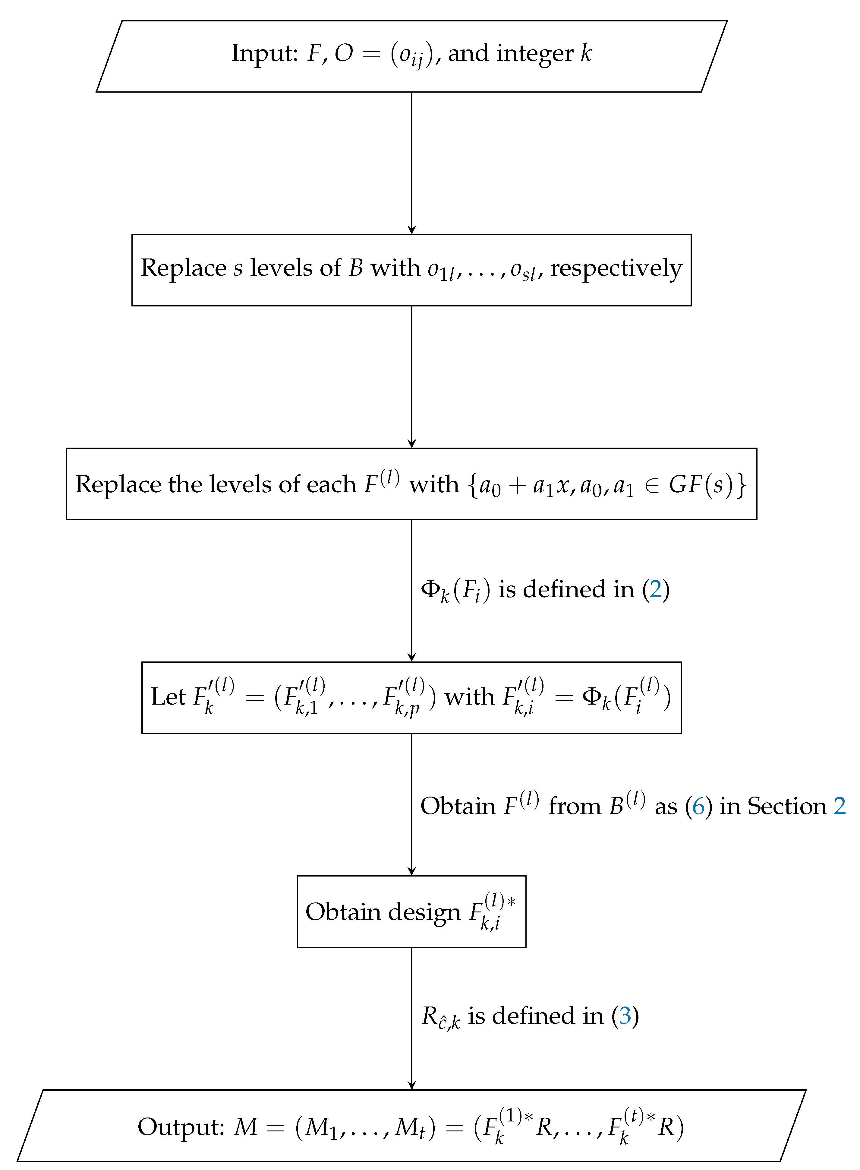
Furthermore, we can construct OLHDs with more columns through Algorithm 2. The flowchart of Algorithm 2 is shown in Appendix B.

Algorithm 2 Enlarging the columns of OLHDs

Input:  $F=(F_1,\dots ,F_p)$, $O=\left(o_{ij}\right)$, and integer k.  1:  Let $O=\left(o_{ij}\right)$ be an OLHD$(s,t)$. For $l=1,\dots ,t$, obtain matrix $B^{\left(l\right)} = (B_1^{\left(l\right)}$, $\dots ,B_p^{\left(l\right)})$ by replacing the s levels of B with $o_{1l},\dots ,o_{sl}$, respectively, where B = $(B_1,\dots ,B_p)$ is the same as in Section 2.  2:  For $l=1,\dots ,t$, obtain $F^{\left(l\right)}$ from $B^{\left(l\right)}$ per (6) in Section 2 and replace the levels of each $F^{\left(l\right)}$ with $\{a_0+a_{1}x,a_0,a_1\in GF\left(s\right)\}$.  3:  For a given integer k and $l=1,\dots ,t$, let $F_k^{{}^{\prime }\left(l\right)}=(F_{k,1}^{{}^{\prime }\left(l\right)},\dots ,F_{k,p}^{{}^{\prime }\left(l\right)})$ with $F_{k,i}^{{}^{\prime }\left(l\right)}={\Phi }_k\left(F_i^{{}^{\prime }\left(l\right)}\right)$ for $i=1,\dots ,p$, where ${\Phi }_k\left(F_i^{\left(l\right)}\right)$ is defined in (2).  4:  For $l=1,\dots ,t$, replace the levels of $F_{k,i}^{{}^{\prime }\left(l\right)}$ with entries from $\Omega \left\{s^2\right\}$ in (1) and denote the resulting design as $F_{k,i}^{\left(l\right)*}$. Construct $M=(M_1,\dots ,M_t)=$ $(F_k^{\left(1\right)*}R,\dots ,F_k^{\left(t\right)*}R)$, where $R={\mathbf{I}}_{p\lfloor s^2/2\rfloor }\otimes R_{\widehat{c},k}$, $\widehat{c}={log}_{2}d-1$, and $R_{\widehat{c},k}$ is the same as in Algorithm 1. Output:  Design M.

Corollary 1. 

Design M obtained by Algorithm 2 is an OLHD$(s^{d+2k},mt)$ where $m=pd\gamma /2$ and $\gamma ={\lfloor s^2/2\rfloor }^k{2}^k$. Each sub-design $M_i$ achieves the same stratifications with Z in Algorithm olhds1 for $i=1,\dots ,t$. At least $2^{k}pdt(2^{k}pdt-2t)/8$ column pairs of M achieve stratifications on $s\times s$ grids in all the two dimensions.

In Step 1, we can choose OLHDs obtained by [15,19] when $s=$ 5, 7, 11, and 17, respectively. According to Algorithm 2, we can obtain OLHDs with t sub-designs, with each satisfying the same stratification properties in Theorem 1. Moreover, when $s=5$, per Algorithm 2 we can obtain an OLHD$(5^6,3744)$ that can accommodate more columns than OLHD$(5^6,2496)$ in [14] and has more attractive space-filling properties.

4. Construction of Orthogonal Designs

This section introduces three rotation methods for constructing ODs. The first two methods can construct ODs with $s^6$ and $s^4$ levels, respectively, while the third can obtain mixed-level ODs. We first present the construction of ODs with $s^6$ levels and investigate their properties. The construction method is provided in Algorithm 3, and the flowchart is shown in Appendix B.

Algorithm 3 Construction of $s^6$-level ODs

Input:  $F=(F_1,\dots ,F_p)$ and $D(s^2,s^2,s^2)=(d_1,$ $\dots ,d_{s^2})$.  1:  Let $F=(F_1,\dots ,F_p)=({\xi }_1,\dots ,{\xi }_{pq})$ with $q=\lfloor d/2\rfloor$, and let D be a difference scheme $D(s^2,s^2,s^2)=(d_1,$ $\dots ,d_{s^2})$ with entries from $GF\left(s^2\right)$ as defined in Section 2. Replace the levels of $\{0,1,\dots ,$ $s^2-1\}$ in each $F_i$ with $\{a_0+a_{1}x,a_0,a_1\in GF\left(s\right)\}$ and define $$E_i=D\oplus {\xi }_i=(d_1\oplus {\xi }_i,\dots ,d_{s^2}\oplus {\xi }_i),i=1,\dots ,pq,q=\lfloor d/2\rfloor .$$  2:  Divide each $E_i$ into g or $g+1$ groups for $i=1,\dots ,pq$ as $E_i=$ $(E_{i,1},\dots ,E_{i,g})$ if $s^2=2g$ or $E_i=(E_{i,1},\dots ,E_{i,g},l_i)$ if $s^2=2g+1,$ where each $E_{i,j}$ has two columns. Then, order $E_{i,j}$’s as $$E_{1,1},E_{2,1},\dots ,E_{pq,1},E_{1,2},E_{2,2},\dots ,E_{pq,2},\dots ,E_{1,g},E_{2,g},\dots ,E_{pq,g}.$$ (8)  3:  Replace the levels of each $E_{i,j}$ with entries from $\Omega \left(s^2\right)$ and denote the resulting design as $E_{i,j}^{*}$. Take two successive instances of $E_{i,j}^{*}$ at a time in the order given in (8), and obtain $\mu =pqg/2$ sets of four columns, denoted as $E^{\left(1\right)},\dots ,E^{\left(\mu \right)}$. Combine $E^{\left(i\right)}$ for $i=1,\dots ,\mu$ together: $$E^{*}=(E^{\left(1\right)},\dots ,E^{\left(\mu \right)}).$$  4:  Create $$X^{*}=(E^{\left(1\right)}{R}_{1,1},\dots ,E^{\left(\mu \right)}{R}_{1,1}),$$ (9) where $$R_{1,1}=\left(\begin{array}{cccc}{s}^4& -s^2& -1& 0\\ s^2& s^4& 0& 1\\ 1& 0& s^4& -s^2\\ 0& -1& s^2& s^4\end{array}\right)$$ is a rotation matrix up to a constant. Output:  Design $X^{*}$.

Based on the form of the rotation matrix, it is easy to see that any column x in $X^{*}$ obtained in (9) has the following form:

$$x=s^{4}e\pm s^2{e}^{\prime }\pm e^{″},$$

(10)

where e and $e^{\prime }$ are the two columns in some $E_{i,j}^{*}$ with $E_{i,j}^{*}\in E^{\left(l\right)}$ for some l; here, $e^{″}$ is a column which is not in $E_{i,j}^{*}$. We call e the leading column of x to facilitate later study. Now, we can consider the mapping

$${\delta }_1\left(z\right)=\lfloor \frac{z+(s^6-1)/2}{s^4}\rfloor -\frac{s^2-1}{2},\mathrm{for}z\in \Omega \left(s^6\right),$$

(11)

with ${\delta }_1(·)$ collapsing the $s^6$ levels in $\Omega \left(s^6\right)$ into $s^2$ levels in $\Omega \left(s^2\right)$. For example, when $s=2$, the 64 levels are collapsed into 4 levels by the mapping, as follows:

$$\begin{array}{cccccc}-31.5,& -30.5,& \dots ,& -16.5& \to & -1.5,\\ -15.5,& -14,5,& \dots ,& -0.5& \to & -0.5,\\ 0.5,& 1,5,& \dots ,& 15.5& \to & 0.5,\\ 16.5,& 17.5& \dots ,& 31.5& \to & 1.5.\end{array}$$

Then, we consider the mapping

$${\delta }_2\left(z\right)=\lfloor \frac{z+(s^6-1)/2}{s^2}\rfloor -\frac{s^4-1}{2},\mathrm{for}z\in \Omega \left(s^6\right),$$

(12)

with ${\delta }_2(·)$ collapsing the $s^6$ levels in $\Omega \left(s^6\right)$ into $s^4$ levels in $\Omega \left(s^4\right)$. For example, when $s=2$, the 64 levels are collapsed into 16 levels by the mapping, as follows:

$$\begin{array}{cccccc}-31.5,& -30.5,& -29.5,& -28.5& \to & -7.5,\\ -27.5,& -26,5,& -25.5,& -24.5& \to & -6.5,\\ ⋮& ⋮& ⋮& ⋮& ⋮& ⋮\\ 24,5,& 25,5,& 26.5,& 27.5& \to & 6.5,\\ 28.5,& 28.5& 30.5,& 31.5& \to & 7.5.\end{array}$$

The resulting design $X^{*}$ is orthogonal and achieves stratifications on $s^2\times s$ or $s\times s^2$ grids; most column pairs can achieve stratifications on $s^2\times s^2$ grids. Moreover, column pairs can achieve stratifications on $s^2\times s^4$ and $s^4\times s^2$ grids as well. We can summarize the properties of $X^{*}$ in the following theorem.

Theorem 2. 

Design $X^{*}$ in (9) is an OD$(s^{d+2},{\left(s^6\right)}^{4\mu })$, where $\mu =\lfloor pqg/2\rfloor$ and $g=\lfloor s^2/2\rfloor$; $X^{*}$ can be partitioned into $pq$ disjoint groups of $2g$ columns, each with the following properties:

(1)

Any two distinct columns achieve a stratification on an $s^2\times s$ or $s\times s^2$ grid;

(2)

Most column pairs achieve stratifications on $s^2\times s^2$ grids, and the proportion ${\pi }_{\alpha }$ is not less than $1-2(s-1)/(4\mu -1)$;

(3)

The proportion of column pairs achieving stratifications on $s^2\times s^4$ and $s^4\times s^2$ grids satisfies ${\pi }_{\beta }\ge 1-(\mu /g+4gs-2g-2s)/(4\mu -1)$.

From Theorem 2, it can be understood that the obtained ODs have appealing stratification properties. For example, for $s=3$ and $d=4$ at least $97.48\%$ of all column pairs of $X^{*}$ can achieve stratifications on $s^2\times s^2$ grids. Furthermore, many column pairs of $X^{*}$ achieve stratifications on finer $s^2\times s^4$ and $s^4\times s^2$ grids (${\pi }_{\beta }\ge 64.78$). The lower bound of this proportion is relatively loose. Below, we provide an illustrative example.

Example 3. 

Consider the same conditions in Example 2 with $p=3$, $q=2$, and $g=2$; we can obtain $F=(F_1,F_2,F_3)=({\xi }_1,\dots ,{\xi }_6)$ and the difference scheme $D(4,4,4)$. From Step 1, we have $E=(E_1,\dots ,E_6)$, where

$$E_i=D\oplus {\xi }_i=(d_0\oplus {\xi }_i,\dots ,d_3\oplus {\xi }_i),i=1,\dots ,6.$$

Then, we divide $E_i$ into two groups, as follows: $E_i=(E_{i,1},E_{i,2})$ for $i=1,\dots ,6$, where each $E_{i,j}$ has two columns, and order the $E_{i,j}$ as follows:

$$E_{1,1},E_{2,1},\dots ,E_{6,1},E_{1,2},E_{2,2},\dots ,E_{6,2}.$$

(13)

We replace the levels of each $E_{i,j}$ with entries from $\Omega \left(s^2\right)$ and denote the resulting design as $E_{i,j}^{*}$. Taking two successive instances of $E_{i,j}^{*}$ at a time in the order given in (13), we obtain $\mu =6$ sets of four columns, denoted as $E^{\left(1\right)},\dots ,E^{\left(6\right)}$. Then, we can obtain an OLHD$(64,24)$ through

$$X^{*}=(E^{\left(1\right)}{R}_{1,1},\dots ,E^{\left(6\right)}{R}_{1,1}),$$

which is displayed in

Table A2. The OLHD$(64,24)$ used in Example 3.

	1	2	3	4	5	6	7	8	9	10	11	12	13	14	15	16	17	18	19	20	21	22	23	24
1	−31.5	−16.5	−28.5	−19.5	−31.5	−16.5	−28.5	−19.5	−31.5	−16.5	−28.5	−19.5	−31.5	−16.5	−28.5	−19.5	−31.5	−16.5	−28.5	−19.5	−31.5	−16.5	−28.5	−19.5
2	−30.5	−17.5	−8.5	−7.5	−28.5	−19.5	31.5	16.5	−10.5	−5.5	−9.5	−6.5	−30.5	−17.5	−8.5	−7.5	−28.5	−19.5	31.5	16.5	−10.5	−5.5	−9.5	−6.5
3	−29.5	−18.5	11.5	4.5	−9.5	−6.5	10.5	5.5	11.5	4.5	29.5	18.5	−29.5	−18.5	11.5	4.5	−9.5	−6.5	10.5	5.5	11.5	4.5	29.5	18.5
4	−28.5	−19.5	31.5	16.5	−10.5	−5.5	−9.5	−6.5	30.5	17.5	8.5	7.5	−28.5	−19.5	31.5	16.5	−10.5	−5.5	−9.5	−6.5	30.5	17.5	8.5	7.5
5	−11.5	−4.5	−29.5	−18.5	29.5	18.5	−11.5	−4.5	−8.5	−7.5	30.5	17.5	−11.5	−4.5	−29.5	−18.5	29.5	18.5	−11.5	−4.5	−8.5	−7.5	30.5	17.5
6	−10.5	−5.5	−9.5	−6.5	30.5	17.5	8.5	7.5	−29.5	−18.5	11.5	4.5	−10.5	−5.5	−9.5	−6.5	30.5	17.5	8.5	7.5	−29.5	−18.5	11.5	4.5
7	−9.5	−6.5	10.5	5.5	11.5	4.5	29.5	18.5	28.5	19.5	−31.5	−16.5	−9.5	−6.5	10.5	5.5	11.5	4.5	29.5	18.5	28.5	19.5	−31.5	−16.5
8	−8.5	−7.5	30.5	17.5	8.5	7.5	−30.5	−17.5	9.5	6.5	−10.5	−5.5	−8.5	−7.5	30.5	17.5	8.5	7.5	−30.5	−17.5	9.5	6.5	−10.5	−5.5
9	8.5	7.5	−30.5	−17.5	9.5	6.5	−10.5	−5.5	10.5	5.5	9.5	6.5	8.5	7.5	−30.5	−17.5	9.5	6.5	−10.5	−5.5	10.5	5.5	9.5	6.5
10	9.5	6.5	−10.5	−5.5	10.5	5.5	9.5	6.5	31.5	16.5	28.5	19.5	9.5	6.5	−10.5	−5.5	10.5	5.5	9.5	6.5	31.5	16.5	28.5	19.5
11	10.5	5.5	9.5	6.5	31.5	16.5	28.5	19.5	−30.5	−17.5	−8.5	−7.5	10.5	5.5	9.5	6.5	31.5	16.5	28.5	19.5	−30.5	−17.5	−8.5	−7.5
12	11.5	4.5	29.5	18.5	28.5	19.5	−31.5	−16.5	−11.5	−4.5	−29.5	−18.5	11.5	4.5	29.5	18.5	28.5	19.5	−31.5	−16.5	−11.5	−4.5	−29.5	−18.5
13	28.5	19.5	−31.5	−16.5	−11.5	−4.5	−29.5	−18.5	29.5	18.5	−11.5	−4.5	28.5	19.5	−31.5	−16.5	−11.5	−4.5	−29.5	−18.5	29.5	18.5	−11.5	−4.5
14	29.5	18.5	−11.5	−4.5	−8.5	−7.5	30.5	17.5	8.5	7.5	−30.5	−17.5	29.5	18.5	−11.5	−4.5	−8.5	−7.5	30.5	17.5	8.5	7.5	−30.5	−17.5
15	30.5	17.5	8.5	7.5	−29.5	−18.5	11.5	4.5	−9.5	−6.5	10.5	5.5	30.5	17.5	8.5	7.5	−29.5	−18.5	11.5	4.5	−9.5	−6.5	10.5	5.5
16	31.5	16.5	28.5	19.5	−30.5	−17.5	−8.5	−7.5	−28.5	−19.5	31.5	16.5	31.5	16.5	28.5	19.5	−30.5	−17.5	−8.5	−7.5	−28.5	−19.5	31.5	16.5
17	−27.5	−1.5	−24.5	−2.5	−27.5	−1.5	−24.5	−2.5	−27.5	−1.5	−24.5	−2.5	14.5	20.5	13.5	23.5	14.5	20.5	13.5	23.5	14.5	20.5	13.5	23.5
18	−26.5	−0.5	−12.5	−22.5	−24.5	−2.5	27.5	1.5	−14.5	−20.5	−13.5	−23.5	15.5	21.5	25.5	3.5	13.5	23.5	−14.5	−20.5	27.5	1.5	24.5	2.5
19	−25.5	−3.5	15.5	21.5	−13.5	−23.5	14.5	20.5	15.5	21.5	25.5	3.5	12.5	22.5	−26.5	−0.5	24.5	2.5	−27.5	−1.5	−26.5	−0.5	−12.5	−22.5
20	−24.5	−2.5	27.5	1.5	−14.5	−20.5	−13.5	−23.5	26.5	0.5	12.5	22.5	13.5	23.5	−14.5	−20.5	27.5	1.5	24.5	2.5	−15.5	−21.5	−25.5	−3.5
21	−15.5	−21.5	−25.5	−3.5	25.5	3.5	−15.5	−21.5	−12.5	−22.5	26.5	0.5	26.5	0.5	12.5	22.5	−12.5	−22.5	26.5	0.5	25.5	3.5	−15.5	−21.5
22	−14.5	−20.5	−13.5	−23.5	26.5	0.5	12.5	22.5	−25.5	−3.5	15.5	21.5	27.5	1.5	24.5	2.5	−15.5	−21.5	−25.5	−3.5	12.5	22.5	−26.5	−0.5
23	−13.5	−23.5	14.5	20.5	15.5	21.5	25.5	3.5	24.5	2.5	−27.5	−1.5	24.5	2.5	−27.5	−1.5	−26.5	−0.5	−12.5	−22.5	−13.5	−23.5	14.5	20.5
24	−12.5	−22.5	26.5	0.5	12.5	22.5	−26.5	−0.5	13.5	23.5	−14.5	−20.5	25.5	3.5	−15.5	−21.5	−25.5	−3.5	15.5	21.5	−24.5	−2.5	27.5	1.5
25	12.5	22.5	−26.5	−0.5	13.5	23.5	−14.5	−20.5	14.5	20.5	13.5	23.5	−25.5	−3.5	15.5	21.5	−24.5	−2.5	27.5	1.5	−27.5	−1.5	−24.5	−2.5
26	13.5	23.5	−14.5	−20.5	14.5	20.5	13.5	23.5	27.5	1.5	24.5	2.5	−24.5	−2.5	27.5	1.5	−27.5	−1.5	−24.5	−2.5	−14.5	−20.5	−13.5	−23.5
27	14.5	20.5	13.5	23.5	27.5	1.5	24.5	2.5	−26.5	−0.5	−12.5	−22.5	−27.5	−1.5	−24.5	−2.5	−14.5	−20.5	−13.5	−23.5	15.5	21.5	25.5	3.5
28	15.5	21.5	25.5	3.5	24.5	2.5	−27.5	−1.5	−15.5	−21.5	−25.5	−3.5	−26.5	−0.5	−12.5	−22.5	−13.5	−23.5	14.5	20.5	26.5	0.5	12.5	22.5
29	24.5	2.5	−27.5	−1.5	−15.5	−21.5	−25.5	−3.5	25.5	3.5	−15.5	−21.5	−13.5	−23.5	14.5	20.5	26.5	0.5	12.5	22.5	−12.5	−22.5	26.5	0.5
30	25.5	3.5	−15.5	−21.5	−12.5	−22.5	26.5	0.5	12.5	22.5	−26.5	−0.5	−12.5	−22.5	26.5	0.5	25.5	3.5	−15.5	−21.5	−25.5	−3.5	15.5	21.5
31	26.5	0.5	12.5	22.5	−25.5	−3.5	15.5	21.5	−13.5	−23.5	14.5	20.5	−15.5	−21.5	−25.5	−3.5	12.5	22.5	−26.5	−0.5	24.5	2.5	−27.5	−1.5
32	27.5	1.5	24.5	2.5	−26.5	−0.5	−12.5	−22.5	−24.5	−2.5	27.5	1.5	−14.5	−20.5	−13.5	−23.5	15.5	21.5	25.5	3.5	13.5	23.5	−14.5	−20.5
33	−23.5	13.5	−20.5	14.5	−23.5	13.5	−20.5	14.5	−23.5	13.5	−20.5	14.5	23.5	−13.5	20.5	−14.5	23.5	−13.5	20.5	−14.5	23.5	−13.5	20.5	−14.5
34	−22.5	12.5	−0.5	26.5	−20.5	14.5	23.5	−13.5	−2.5	24.5	−1.5	27.5	22.5	−12.5	0.5	−26.5	20.5	−14.5	−23.5	13.5	2.5	−24.5	1.5	−27.5
35	−21.5	15.5	3.5	−25.5	−1.5	27.5	2.5	−24.5	3.5	−25.5	21.5	−15.5	21.5	−15.5	−3.5	25.5	1.5	−27.5	−2.5	24.5	−3.5	25.5	−21.5	15.5
36	−20.5	14.5	23.5	−13.5	−2.5	24.5	−1.5	27.5	22.5	−12.5	0.5	−26.5	20.5	−14.5	−23.5	13.5	2.5	−24.5	1.5	−27.5	−22.5	12.5	−0.5	26.5
37	−3.5	25.5	−21.5	15.5	21.5	−15.5	−3.5	25.5	−0.5	26.5	22.5	−12.5	3.5	−25.5	21.5	−15.5	−21.5	15.5	3.5	−25.5	0.5	−26.5	−22.5	12.5
38	−2.5	24.5	−1.5	27.5	22.5	−12.5	0.5	−26.5	−21.5	15.5	3.5	−25.5	2.5	−24.5	1.5	−27.5	−22.5	12.5	−0.5	26.5	21.5	−15.5	−3.5	25.5
39	−1.5	27.5	2.5	−24.5	3.5	−25.5	21.5	−15.5	20.5	−14.5	−23.5	13.5	1.5	−27.5	−2.5	24.5	−3.5	25.5	−21.5	15.5	−20.5	14.5	23.5	−13.5
40	−0.5	26.5	22.5	−12.5	0.5	−26.5	−22.5	12.5	1.5	−27.5	−2.5	24.5	0.5	−26.5	−22.5	12.5	−0.5	26.5	22.5	−12.5	−1.5	27.5	2.5	−24.5
41	0.5	−26.5	−22.5	12.5	1.5	−27.5	−2.5	24.5	2.5	−24.5	1.5	−27.5	−0.5	26.5	22.5	−12.5	−1.5	27.5	2.5	−24.5	−2.5	24.5	−1.5	27.5
42	1.5	−27.5	−2.5	24.5	2.5	−24.5	1.5	−27.5	23.5	−13.5	20.5	−14.5	−1.5	27.5	2.5	−24.5	−2.5	24.5	−1.5	27.5	−23.5	13.5	−20.5	14.5
43	2.5	−24.5	1.5	−27.5	23.5	−13.5	20.5	−14.5	−22.5	12.5	−0.5	26.5	−2.5	24.5	−1.5	27.5	−23.5	13.5	−20.5	14.5	22.5	−12.5	0.5	−26.5
44	3.5	−25.5	21.5	−15.5	20.5	−14.5	−23.5	13.5	−3.5	25.5	−21.5	15.5	−3.5	25.5	−21.5	15.5	−20.5	14.5	23.5	−13.5	3.5	−25.5	21.5	−15.5
45	20.5	−14.5	−23.5	13.5	−3.5	25.5	−21.5	15.5	21.5	−15.5	−3.5	25.5	−20.5	14.5	23.5	−13.5	3.5	−25.5	21.5	−15.5	−21.5	15.5	3.5	−25.5
46	21.5	−15.5	−3.5	25.5	−0.5	26.5	22.5	−12.5	0.5	−26.5	−22.5	12.5	−21.5	15.5	3.5	−25.5	0.5	−26.5	−22.5	12.5	−0.5	26.5	22.5	−12.5
47	22.5	−12.5	0.5	−26.5	−21.5	15.5	3.5	−25.5	−1.5	27.5	2.5	−24.5	−22.5	12.5	−0.5	26.5	21.5	−15.5	−3.5	25.5	1.5	−27.5	−2.5	24.5
48	23.5	−13.5	20.5	−14.5	−22.5	12.5	−0.5	26.5	−20.5	14.5	23.5	−13.5	−23.5	13.5	−20.5	14.5	22.5	−12.5	0.5	−26.5	20.5	−14.5	−23.5	13.5
49	−19.5	28.5	−16.5	31.5	−19.5	28.5	−16.5	31.5	−19.5	28.5	−16.5	31.5	−6.5	9.5	−5.5	10.5	−6.5	9.5	−5.5	10.5	−6.5	9.5	−5.5	10.5
50	−18.5	29.5	−4.5	11.5	−16.5	31.5	19.5	−28.5	−6.5	9.5	−5.5	10.5	−7.5	8.5	−17.5	30.5	−5.5	10.5	6.5	−9.5	−19.5	28.5	−16.5	31.5
51	−17.5	30.5	7.5	−8.5	−5.5	10.5	6.5	−9.5	7.5	−8.5	17.5	−30.5	−4.5	11.5	18.5	−29.5	−16.5	31.5	19.5	−28.5	18.5	−29.5	4.5	−11.5
52	−16.5	31.5	19.5	−28.5	−6.5	9.5	−5.5	10.5	18.5	−29.5	4.5	−11.5	−5.5	10.5	6.5	−9.5	−19.5	28.5	−16.5	31.5	7.5	−8.5	17.5	−30.5
53	−7.5	8.5	−17.5	30.5	17.5	−30.5	−7.5	8.5	−4.5	11.5	18.5	−29.5	−18.5	29.5	−4.5	11.5	4.5	−11.5	−18.5	29.5	−17.5	30.5	7.5	−8.5
54	−6.5	9.5	−5.5	10.5	18.5	−29.5	4.5	−11.5	−17.5	30.5	7.5	−8.5	−19.5	28.5	−16.5	31.5	7.5	−8.5	17.5	−30.5	−4.5	11.5	18.5	−29.5
55	−5.5	10.5	6.5	−9.5	7.5	−8.5	17.5	−30.5	16.5	−31.5	−19.5	28.5	−16.5	31.5	19.5	−28.5	18.5	−29.5	4.5	−11.5	5.5	−10.5	−6.5	9.5
56	−4.5	11.5	18.5	−29.5	4.5	−11.5	−18.5	29.5	5.5	−10.5	−6.5	9.5	−17.5	30.5	7.5	−8.5	17.5	−30.5	−7.5	8.5	16.5	−31.5	−19.5	28.5
57	4.5	−11.5	−18.5	29.5	5.5	−10.5	−6.5	9.5	6.5	−9.5	5.5	−10.5	17.5	−30.5	−7.5	8.5	16.5	−31.5	−19.5	28.5	19.5	−28.5	16.5	−31.5
58	5.5	−10.5	−6.5	9.5	6.5	−9.5	5.5	−10.5	19.5	−28.5	16.5	−31.5	16.5	−31.5	−19.5	28.5	19.5	−28.5	16.5	−31.5	6.5	−9.5	5.5	−10.5
59	6.5	−9.5	5.5	−10.5	19.5	−28.5	16.5	−31.5	−18.5	29.5	−4.5	11.5	19.5	−28.5	16.5	−31.5	6.5	−9.5	5.5	−10.5	−7.5	8.5	−17.5	30.5
60	7.5	−8.5	17.5	−30.5	16.5	−31.5	−19.5	28.5	−7.5	8.5	−17.5	30.5	18.5	−29.5	4.5	−11.5	5.5	−10.5	−6.5	9.5	−18.5	29.5	−4.5	11.5
61	16.5	−31.5	−19.5	28.5	−7.5	8.5	−17.5	30.5	17.5	−30.5	−7.5	8.5	5.5	−10.5	−6.5	9.5	−18.5	29.5	−4.5	11.5	4.5	−11.5	−18.5	29.5
62	17.5	−30.5	−7.5	8.5	−4.5	11.5	18.5	−29.5	4.5	−11.5	−18.5	29.5	4.5	−11.5	−18.5	29.5	−17.5	30.5	7.5	−8.5	17.5	−30.5	−7.5	8.5
63	18.5	−29.5	4.5	−11.5	−17.5	30.5	7.5	−8.5	−5.5	10.5	6.5	−9.5	7.5	−8.5	17.5	−30.5	−4.5	11.5	18.5	−29.5	−16.5	31.5	19.5	−28.5
64	19.5	−28.5	16.5	−31.5	−18.5	29.5	−4.5	11.5	−16.5	31.5	19.5	−28.5	6.5	−9.5	5.5	−10.5	−7.5	8.5	−17.5	30.5	−5.5	10.5	6.5	−9.5

of Appendix B. The stratification properties of $X^{*}$ are summarized in

Table 6. The stratification properties of the resulting OLHD$(64,24)$ in Example 3.

	$4\times 16$	$16\times 4$	$2\times 4$	$4\times 2$	$4\times 4$
count	176	176	272	264	260
proportion (%)	63.77	63.77	98.55	95.65	94.20

. It can be seen that this design has the same number of column pairs achieving stratification on a $4\times 4$ grid as the one in Example 2, and has more column pairs achieving stratifications on $4\times 16$ or $16\times 4$ grids than the one in Example 2 with ${\pi }_{\beta }=63.77\%$. Furthermore, by calculation, we can say that the obtained OLHD$(64,24)$ achieves stratifications on a $2\times 32$ grid in 140 out of all 276 (i.e., $50.72\%$) and on a $32\times 2$ grid in100 out of all 276 (i.e., $36.23\%$).

The OAs and difference schemes used in the construction are available in [20] and the library of OAs (http://neilsloane.com/oadir/index.html, accessed on 16 March 2023). It is easy to show that $X^{*}$ is an OLHD$(s^{d+2},4\mu )$ when $d=4$.

Table 7. Example ODs constructed by Algorithm 3.

s	d	p	q	g	OA$({\mathit{s}}^{\mathit{d}},\frac{{\mathit{s}}^{\mathit{d}}-1}{\mathit{s}-1},\mathit{s},2)$	OD$({\mathit{s}}^{\mathit{d}+2},{\left({\mathit{s}}^6\right)}^{4\mathit{\mu }})$	${\mathit{\pi }}_{\mathit{\alpha },\mathit{LB}}$	${\mathit{\pi }}_{\mathit{\beta },\mathit{LB}}$
2	4	3	2	2	OA$(2^4,15,2,2)$	OD$(2^6,{\left(64\right)}^{24})\#$	91.30	39.13
2	5	6	2	2	OA$(2^5,31,2,2)$	OD$(2^7,{\left(64\right)}^{48})$	95.74	57.45
2	6	10	3	2	OA$(2^6,63,2,2)$	OD$(2^8,{\left(64\right)}^{120})$	98.32	68.07
2	7	18	3	2	OA$(2^7,127,2,2)$	OD$(2^9,{\left(64\right)}^{216})$	99.07	71.16
2	8	31	4	2	OA$(2^8,255,2,2)$	OD$(2^{10},{\left(64\right)}^{496})$	99.60	73.33
3	4	10	2	4	OA$(3^4,40,3,2)$	OD$(3^6,{\left(729\right)}^{160})\#$	97.48	64.78
3	5	24	2	4	OA$(3^5,121,3,2)$	OD$(3^7,{\left(729\right)}^{384})$	98.96	78.07
3	6	60	3	4	OA$(3^6,364,3,2)$	OD$(3^8,{\left(729\right)}^{1440})$	99.72	84.99
3	7	156	3	4	OA$(3^7,1093,3,2)$	OD$(3^9,{\left(729\right)}^{3744})$	99.89	86.53
5	4	39	2	12	OA$(5^4,156,5,2)$	OD$(5^6,{\left(15625\right)}^{1872})\#$	99.57	84.82

The # symbol indicates that the design is also an OLHD.

summarizes example ODs constructed by Algorithm 3. Their space-filling properties are characterized by ${\pi }_{\alpha }$ and ${\pi }_{\beta }$. Similar to Section 3, we only list the lower bounds of ${\pi }_{\alpha }$ and ${\pi }_{\beta }$ in Table 7, denoted as ${\pi }_{\alpha ,LB}$ and ${\pi }_{\beta ,LB}$, respectively. As shown in Table 7, the lower bounds of ${\pi }_{\alpha }$ are very close to 1 and those of ${\pi }_{\beta }$ are quite large in most cases, which means that nearly all the column pairs of these ODs achieve stratifications on $s^2\times s^2$ grids, and that most column pairs achieve stratifications on finer $s^2\times s^4$ and $s^4\times s^2$ grids as well.

Next, we introduce the construction of ODs with $s^4$ levels with the same space-filling properties as the designs obtained in Algorithm 3. The construction method is provided in Algorithm 4.

Algorithm 4 Construction of $s^4$-level ODs

Input:  $F=(F_1,\dots ,F_p)$ and $D(s^2,s^2,s^2)=(d_1,$ $\dots ,d_{s^2})$.  1:  Let matrices B, F, D, $E_{i,j}$, $E_{i,j}^{*}$ be the same as in Algorithm 3.  2:  For $i=1,\dots ,pd/2$, define $G_i=(E_{i,1}^{*},\dots ,E_{i,g}^{*})$ with $g=\lfloor s^2/2\rfloor$.  3:  Create $$Y=(G_1,\dots ,G_{pd/2})V=(Y_1,\dots ,Y_{pd/2}),$$ (14) where $$V=\left(\begin{array}{cccc}{R}_{1,0}& 0_{2\times 2}& \cdots & 0_{2\times 2}\\ 0_{2\times 2}& R_{1,0}& \cdots & 0_{2\times 2}\\ ⋮& ⋮& \ddots & ⋮\\ 0_{2\times 2}& 0_{2\times 2}& \cdots & R_{1,0}\end{array}\right)\mathrm{with}{R}_{1,0}=\left(\begin{array}{cc}{s}^2& -1\\ 1& s^2\end{array}\right),$$ where $R_{1,0}$ is repeated $pdg/2$ times and all off-diagonal sub-matrices of V are $2\times 2$ zero matrices. Output:  Design Y.

For the resulting design, it is easy to obtain the following theorem.

Theorem 3. 

Design Y in (14) is an OD$(s^{d+2},{\left(s^4\right)}^m)$ with $m=2pdg$, $g=\lfloor s^2/2\rfloor$ that can be partitioned into $pd$ disjoint groups of $2g$ columns with the same stratification properties as $X^{*}$ in Theorem 2.

Compared with the ODs constructed in Algorithm 3, design Y has lower levels and can accommodate more columns than design $X^{*}$ in Algorithm 3 when d is an odd number. Now, we turn to an illustrative example.

Example 4. 

Considering the same conditions in Example 3, we first obtain the E_i,js. For $i=1,\dots ,6$, we define $G_i=(E_{i,1}^{*},E_{i,2}^{*})$ and $R_{1,0}=\left(\begin{array}{cc}{s}^2& -1\\ 1& s^2\end{array}\right)$. We can construct an OD$(64,{16}^{24})$ by

$$Y=(Y_1,\dots ,Y_6)=(G_1,\dots ,G_6)V,$$

which is displayed in

Table A3. The OD$(64,{16}^{24})$ used in Example 4.

	1	2	3	4	5	6	7	8	9	10	11	12	13	14	15	16	17	18	19	20	21	22	23	24
1	−7.5	−4.5	−7.5	−4.5	−7.5	−4.5	−7.5	−4.5	−7.5	−4.5	−7.5	−4.5	−7.5	−4.5	−7.5	−4.5	−7.5	−4.5	−7.5	−4.5	−7.5	−4.5	−7.5	−4.5
2	−7.5	−4.5	−2.5	−1.5	−7.5	−4.5	7.5	4.5	−2.5	−1.5	−2.5	−1.5	−7.5	−4.5	−2.5	−1.5	−7.5	−4.5	7.5	4.5	−2.5	−1.5	−2.5	−1.5
3	−7.5	−4.5	2.5	1.5	−2.5	−1.5	2.5	1.5	2.5	1.5	7.5	4.5	−7.5	−4.5	2.5	1.5	−2.5	−1.5	2.5	1.5	2.5	1.5	7.5	4.5
4	−7.5	−4.5	7.5	4.5	−2.5	−1.5	−2.5	−1.5	7.5	4.5	2.5	1.5	−7.5	−4.5	7.5	4.5	−2.5	−1.5	−2.5	−1.5	7.5	4.5	2.5	1.5
5	−2.5	−1.5	−7.5	−4.5	7.5	4.5	−2.5	−1.5	−2.5	−1.5	7.5	4.5	−2.5	−1.5	−7.5	−4.5	7.5	4.5	−2.5	−1.5	−2.5	−1.5	7.5	4.5
6	−2.5	−1.5	−2.5	−1.5	7.5	4.5	2.5	1.5	−7.5	−4.5	2.5	1.5	−2.5	−1.5	−2.5	−1.5	7.5	4.5	2.5	1.5	−7.5	−4.5	2.5	1.5
7	−2.5	−1.5	2.5	1.5	2.5	1.5	7.5	4.5	7.5	4.5	−7.5	−4.5	−2.5	−1.5	2.5	1.5	2.5	1.5	7.5	4.5	7.5	4.5	−7.5	−4.5
8	−2.5	−1.5	7.5	4.5	2.5	1.5	−7.5	−4.5	2.5	1.5	−2.5	−1.5	−2.5	−1.5	7.5	4.5	2.5	1.5	−7.5	−4.5	2.5	1.5	−2.5	−1.5
9	2.5	1.5	−7.5	−4.5	2.5	1.5	−2.5	−1.5	2.5	1.5	2.5	1.5	2.5	1.5	−7.5	−4.5	2.5	1.5	−2.5	−1.5	2.5	1.5	2.5	1.5
10	2.5	1.5	−2.5	−1.5	2.5	1.5	2.5	1.5	7.5	4.5	7.5	4.5	2.5	1.5	−2.5	−1.5	2.5	1.5	2.5	1.5	7.5	4.5	7.5	4.5
11	2.5	1.5	2.5	1.5	7.5	4.5	7.5	4.5	−7.5	−4.5	−2.5	−1.5	2.5	1.5	2.5	1.5	7.5	4.5	7.5	4.5	−7.5	−4.5	−2.5	−1.5
12	2.5	1.5	7.5	4.5	7.5	4.5	−7.5	−4.5	−2.5	−1.5	−7.5	−4.5	2.5	1.5	7.5	4.5	7.5	4.5	−7.5	−4.5	−2.5	−1.5	−7.5	−4.5
13	7.5	4.5	−7.5	−4.5	−2.5	−1.5	−7.5	−4.5	7.5	4.5	−2.5	−1.5	7.5	4.5	−7.5	−4.5	−2.5	−1.5	−7.5	−4.5	7.5	4.5	−2.5	−1.5
14	7.5	4.5	−2.5	−1.5	−2.5	−1.5	7.5	4.5	2.5	1.5	−7.5	−4.5	7.5	4.5	−2.5	−1.5	−2.5	−1.5	7.5	4.5	2.5	1.5	−7.5	−4.5
15	7.5	4.5	2.5	1.5	−7.5	−4.5	2.5	1.5	−2.5	−1.5	2.5	1.5	7.5	4.5	2.5	1.5	−7.5	−4.5	2.5	1.5	−2.5	−1.5	2.5	1.5
16	7.5	4.5	7.5	4.5	−7.5	−4.5	−2.5	−1.5	−7.5	−4.5	7.5	4.5	7.5	4.5	7.5	4.5	−7.5	−4.5	−2.5	−1.5	−7.5	−4.5	7.5	4.5
17	−6.5	−0.5	−6.5	−0.5	−6.5	−0.5	−6.5	−0.5	−6.5	−0.5	−6.5	−0.5	3.5	5.5	3.5	5.5	3.5	5.5	3.5	5.5	3.5	5.5	3.5	5.5
18	−6.5	−0.5	−3.5	−5.5	−6.5	−0.5	6.5	0.5	−3.5	−5.5	−3.5	−5.5	3.5	5.5	6.5	0.5	3.5	5.5	−3.5	−5.5	6.5	0.5	6.5	0.5
19	−6.5	−0.5	3.5	5.5	−3.5	−5.5	3.5	5.5	3.5	5.5	6.5	0.5	3.5	5.5	−6.5	−0.5	6.5	0.5	−6.5	−0.5	−6.5	−0.5	−3.5	−5.5
20	−6.5	−0.5	6.5	0.5	−3.5	−5.5	−3.5	−5.5	6.5	0.5	3.5	5.5	3.5	5.5	−3.5	−5.5	6.5	0.5	6.5	0.5	−3.5	−5.5	−6.5	−0.5
21	−3.5	−5.5	−6.5	−0.5	6.5	0.5	−3.5	−5.5	−3.5	−5.5	6.5	0.5	6.5	0.5	3.5	5.5	−3.5	−5.5	6.5	0.5	6.5	0.5	−3.5	−5.5
22	−3.5	−5.5	−3.5	−5.5	6.5	0.5	3.5	5.5	−6.5	−0.5	3.5	5.5	6.5	0.5	6.5	0.5	−3.5	−5.5	−6.5	−0.5	3.5	5.5	−6.5	−0.5
23	−3.5	−5.5	3.5	5.5	3.5	5.5	6.5	0.5	6.5	0.5	−6.5	−0.5	6.5	0.5	−6.5	−0.5	−6.5	−0.5	−3.5	−5.5	−3.5	−5.5	3.5	5.5
24	−3.5	−5.5	6.5	0.5	3.5	5.5	−6.5	−0.5	3.5	5.5	−3.5	−5.5	6.5	0.5	−3.5	−5.5	−6.5	−0.5	3.5	5.5	−6.5	−0.5	6.5	0.5
25	3.5	5.5	−6.5	−0.5	3.5	5.5	−3.5	−5.5	3.5	5.5	3.5	5.5	−6.5	−0.5	3.5	5.5	−6.5	−0.5	6.5	0.5	−6.5	−0.5	−6.5	−0.5
26	3.5	5.5	−3.5	−5.5	3.5	5.5	3.5	5.5	6.5	0.5	6.5	0.5	−6.5	−0.5	6.5	0.5	−6.5	−0.5	−6.5	−0.5	−3.5	−5.5	−3.5	−5.5
27	3.5	5.5	3.5	5.5	6.5	0.5	6.5	0.5	−6.5	−0.5	−3.5	−5.5	−6.5	−0.5	−6.5	−0.5	−3.5	−5.5	−3.5	−5.5	3.5	5.5	6.5	0.5
28	3.5	5.5	6.5	0.5	6.5	0.5	−6.5	−0.5	−3.5	−5.5	−6.5	−0.5	−6.5	−0.5	−3.5	−5.5	−3.5	−5.5	3.5	5.5	6.5	0.5	3.5	5.5
29	6.5	0.5	−6.5	−0.5	−3.5	−5.5	−6.5	−0.5	6.5	0.5	−3.5	−5.5	−3.5	−5.5	3.5	5.5	6.5	0.5	3.5	5.5	−3.5	−5.5	6.5	0.5
30	6.5	0.5	−3.5	−5.5	−3.5	−5.5	6.5	0.5	3.5	5.5	−6.5	−0.5	−3.5	−5.5	6.5	0.5	6.5	0.5	−3.5	−5.5	−6.5	−0.5	3.5	5.5
31	6.5	0.5	3.5	5.5	−6.5	−0.5	3.5	5.5	−3.5	−5.5	3.5	5.5	−3.5	−5.5	−6.5	−0.5	3.5	5.5	−6.5	−0.5	6.5	0.5	−6.5	−0.5
32	6.5	0.5	6.5	0.5	−6.5	−0.5	−3.5	−5.5	−6.5	−0.5	6.5	0.5	−3.5	−5.5	−3.5	−5.5	3.5	5.5	6.5	0.5	3.5	5.5	−3.5	−5.5
33	−5.5	3.5	−5.5	3.5	−5.5	3.5	−5.5	3.5	−5.5	3.5	−5.5	3.5	5.5	−3.5	5.5	−3.5	5.5	−3.5	5.5	−3.5	5.5	−3.5	5.5	−3.5
34	−5.5	3.5	−0.5	6.5	−5.5	3.5	5.5	−3.5	−0.5	6.5	−0.5	6.5	5.5	−3.5	0.5	−6.5	5.5	−3.5	−5.5	3.5	0.5	−6.5	0.5	−6.5
35	−5.5	3.5	0.5	−6.5	−0.5	6.5	0.5	−6.5	0.5	−6.5	5.5	−3.5	5.5	−3.5	−0.5	6.5	0.5	−6.5	−0.5	6.5	−0.5	6.5	−5.5	3.5
36	−5.5	3.5	5.5	−3.5	−0.5	6.5	−0.5	6.5	5.5	−3.5	0.5	−6.5	5.5	−3.5	−5.5	3.5	0.5	−6.5	0.5	−6.5	−5.5	3.5	−0.5	6.5
37	−0.5	6.5	−5.5	3.5	5.5	−3.5	−0.5	6.5	−0.5	6.5	5.5	−3.5	0.5	−6.5	5.5	−3.5	−5.5	3.5	0.5	−6.5	0.5	−6.5	−5.5	3.5
38	−0.5	6.5	−0.5	6.5	5.5	−3.5	0.5	−6.5	−5.5	3.5	0.5	−6.5	0.5	−6.5	0.5	−6.5	−5.5	3.5	−0.5	6.5	5.5	−3.5	−0.5	6.5
39	−0.5	6.5	0.5	−6.5	0.5	−6.5	5.5	−3.5	5.5	−3.5	−5.5	3.5	0.5	−6.5	−0.5	6.5	−0.5	6.5	−5.5	3.5	−5.5	3.5	5.5	−3.5
40	−0.5	6.5	5.5	−3.5	0.5	−6.5	−5.5	3.5	0.5	−6.5	−0.5	6.5	0.5	−6.5	−5.5	3.5	−0.5	6.5	5.5	−3.5	−0.5	6.5	0.5	−6.5
41	0.5	−6.5	−5.5	3.5	0.5	−6.5	−0.5	6.5	0.5	−6.5	0.5	−6.5	−0.5	6.5	5.5	−3.5	−0.5	6.5	0.5	−6.5	−0.5	6.5	−0.5	6.5
42	0.5	−6.5	−0.5	6.5	0.5	−6.5	0.5	−6.5	5.5	−3.5	5.5	−3.5	−0.5	6.5	0.5	−6.5	−0.5	6.5	−0.5	6.5	−5.5	3.5	−5.5	3.5
43	0.5	−6.5	0.5	−6.5	5.5	−3.5	5.5	−3.5	−5.5	3.5	−0.5	6.5	−0.5	6.5	−0.5	6.5	−5.5	3.5	−5.5	3.5	5.5	−3.5	0.5	−6.5
44	0.5	−6.5	5.5	−3.5	5.5	−3.5	−5.5	3.5	−0.5	6.5	−5.5	3.5	−0.5	6.5	−5.5	3.5	−5.5	3.5	5.5	−3.5	0.5	−6.5	5.5	−3.5
45	5.5	−3.5	−5.5	3.5	−0.5	6.5	−5.5	3.5	5.5	−3.5	−0.5	6.5	−5.5	3.5	5.5	−3.5	0.5	−6.5	5.5	−3.5	−5.5	3.5	0.5	−6.5
46	5.5	−3.5	−0.5	6.5	−0.5	6.5	5.5	−3.5	0.5	−6.5	−5.5	3.5	−5.5	3.5	0.5	−6.5	0.5	−6.5	−5.5	3.5	−0.5	6.5	5.5	−3.5
47	5.5	−3.5	0.5	−6.5	−5.5	3.5	0.5	−6.5	−0.5	6.5	0.5	−6.5	−5.5	3.5	−0.5	6.5	5.5	−3.5	−0.5	6.5	0.5	−6.5	−0.5	6.5
48	5.5	−3.5	5.5	−3.5	−5.5	3.5	−0.5	6.5	−5.5	3.5	5.5	−3.5	−5.5	3.5	−5.5	3.5	5.5	−3.5	0.5	−6.5	5.5	−3.5	−5.5	3.5
49	−4.5	7.5	−4.5	7.5	−4.5	7.5	−4.5	7.5	−4.5	7.5	−4.5	7.5	−1.5	2.5	−1.5	2.5	−1.5	2.5	−1.5	2.5	−1.5	2.5	−1.5	2.5
50	−4.5	7.5	−1.5	2.5	−4.5	7.5	4.5	−7.5	−1.5	2.5	−1.5	2.5	−1.5	2.5	−4.5	7.5	−1.5	2.5	1.5	−2.5	−4.5	7.5	−4.5	7.5
51	−4.5	7.5	1.5	−2.5	−1.5	2.5	1.5	−2.5	1.5	−2.5	4.5	−7.5	−1.5	2.5	4.5	−7.5	−4.5	7.5	4.5	−7.5	4.5	−7.5	1.5	−2.5
52	−4.5	7.5	4.5	−7.5	−1.5	2.5	−1.5	2.5	4.5	−7.5	1.5	−2.5	−1.5	2.5	1.5	−2.5	−4.5	7.5	−4.5	7.5	1.5	−2.5	4.5	−7.5
53	−1.5	2.5	−4.5	7.5	4.5	−7.5	−1.5	2.5	−1.5	2.5	4.5	−7.5	−4.5	7.5	−1.5	2.5	1.5	−2.5	−4.5	7.5	−4.5	7.5	1.5	−2.5
54	−1.5	2.5	−1.5	2.5	4.5	−7.5	1.5	−2.5	−4.5	7.5	1.5	−2.5	−4.5	7.5	−4.5	7.5	1.5	−2.5	4.5	−7.5	−1.5	2.5	4.5	−7.5
55	−1.5	2.5	1.5	−2.5	1.5	−2.5	4.5	−7.5	4.5	−7.5	−4.5	7.5	−4.5	7.5	4.5	−7.5	4.5	−7.5	1.5	−2.5	1.5	−2.5	−1.5	2.5
56	−1.5	2.5	4.5	−7.5	1.5	−2.5	−4.5	7.5	1.5	−2.5	−1.5	2.5	−4.5	7.5	1.5	−2.5	4.5	−7.5	−1.5	2.5	4.5	−7.5	−4.5	7.5
57	1.5	−2.5	−4.5	7.5	1.5	−2.5	−1.5	2.5	1.5	−2.5	1.5	−2.5	4.5	−7.5	−1.5	2.5	4.5	−7.5	−4.5	7.5	4.5	−7.5	4.5	−7.5
58	1.5	−2.5	−1.5	2.5	1.5	−2.5	1.5	−2.5	4.5	−7.5	4.5	−7.5	4.5	−7.5	−4.5	7.5	4.5	−7.5	4.5	−7.5	1.5	−2.5	1.5	−2.5
59	1.5	−2.5	1.5	−2.5	4.5	−7.5	4.5	−7.5	−4.5	7.5	−1.5	2.5	4.5	−7.5	4.5	−7.5	1.5	−2.5	1.5	−2.5	−1.5	2.5	−4.5	7.5
60	1.5	−2.5	4.5	−7.5	4.5	−7.5	−4.5	7.5	−1.5	2.5	−4.5	7.5	4.5	−7.5	1.5	−2.5	1.5	−2.5	−1.5	2.5	−4.5	7.5	−1.5	2.5
61	4.5	−7.5	−4.5	7.5	−1.5	2.5	−4.5	7.5	4.5	−7.5	−1.5	2.5	1.5	−2.5	−1.5	2.5	−4.5	7.5	−1.5	2.5	1.5	−2.5	−4.5	7.5
62	4.5	−7.5	−1.5	2.5	−1.5	2.5	4.5	−7.5	1.5	−2.5	−4.5	7.5	1.5	−2.5	−4.5	7.5	−4.5	7.5	1.5	−2.5	4.5	−7.5	−1.5	2.5
63	4.5	−7.5	1.5	−2.5	−4.5	7.5	1.5	−2.5	−1.5	2.5	1.5	−2.5	1.5	−2.5	4.5	−7.5	−1.5	2.5	4.5	−7.5	−4.5	7.5	4.5	−7.5
64	4.5	−7.5	4.5	−7.5	−4.5	7.5	−1.5	2.5	−4.5	7.5	4.5	−7.5	1.5	−2.5	1.5	−2.5	−1.5	2.5	−4.5	7.5	−1.5	2.5	1.5	−2.5

of Appendix B. It can be seen that the design points are well-scattered in the two-dimensional projections of the resulting OD$(64,{16}^{24})$, and it has the same space-filling properties as the OD constructed in Example 3.

Table 8. Example ODs constructed by Algorithm 4.

s	d	p	g	OA$({\mathit{s}}^{\mathit{d}},\frac{{\mathit{s}}^{\mathit{d}}-1}{\mathit{s}-1},\mathit{s},2)$	OD$({\mathit{s}}^{\mathit{d}+2},{\left({\mathit{s}}^4\right)}^{\mathit{m}})$	${\mathit{\pi }}_{\mathit{\alpha },\mathit{LB}}$	${\mathit{\pi }}_{\mathit{\beta },\mathit{LB}}$
2	4	3	2	OA$(2^4,15,2,2)$	OD$(2^6,{\left(16\right)}^{24})$	91.30	39.13
2	5	6	2	OA$(2^5,31,2,2)$	OD$(2^7,{\left(16\right)}^{60})$	95.74	61.02
2	6	10	2	OA$(2^6,63,2,2)$	OD$(2^8,{\left(16\right)}^{120})$	98.32	68.07
2	7	18	2	OA$(2^7,127,2,2)$	OD$(2^9,{\left(16\right)}^{252})$	99.07	71.71
2	8	31	2	OA$(2^8,255,2,2)$	OD$(2^{10},{\left(16\right)}^{496})$	99.60	73.33
3	4	10	4	OA$(3^4,40,3,2)$	OD$(3^6,{\left(81\right)}^{160})$	97.48	64.78
3	5	24	4	OA$(3^5,121,3,2)$	OD$(3^7,{\left(81\right)}^{480})$	98.96	79.96
3	6	60	4	OA$(3^6,364,3,2)$	OD$(3^8,{\left(81\right)}^{1440})$	99.72	84.99
3	7	156	4	OA$(3^7,1093,3,2)$	OD$(3^9,{\left(81\right)}^{4368})$	99.89	86.67
5	3	10	12	OA$(5^3,31,5,2)$	OD$(5^5,{\left(625\right)}^{360})$	96.65	38.44
5	4	39	12	OA$(5^4,156,5,2)$	OD$(5^6,{\left(625\right)}^{1872})$	99.57	84.82

lists example ODs obtained by Algorithm 4. Compared with the ODs constructed using Algorithm 3, the obtained designs have lower levels and more columns when d is odd. The resulting designs have the same stratification properties as the ODs constructed by Algorithm 3. These ODs have more flexible run sizes than the OLHDs obtained by Algorithm 1.

Now, we consider the construction of mixed-level ODs, which are very useful when the factors cannot have the same number of levels. The construction method is provided in Algorithm 5.

Algorithm 5 Construction of mixed-level ODs

Input:  $F=(F_1,\dots ,F_p)$ and $D(s^2,s^2,s^2)=(d_1,$ $\dots ,d_{s^2})$.  1:  Let matrices B, F, D, $E_{i,j}$, and $E_{i,j}^{*}$ be the same as in Algorithm 3. Then, order the Ei,js as in (8). First, take two successive $E_{i,j}$ instances at each time in the above list and take a total of ${\mu }_1$ times (where ${\mu }_1\le \lfloor pqg/2\rfloor$) to ${\mu }_1$ sets of four columns each. Center the $s^2$ levels of each column into $\Omega \left(s^2\right)$ in (1) and denote these sets as $E^{\left(1\right)},\dots ,E^{\left({\mu }_1\right)}$.  2:  Take one $E_{i,j}$ at a time in the remaining list of (8), thus ${\mu }_2=\lfloor pdg/2\rfloor$ $-2{\mu }_1$ sets of two columns each can be obtained. Similarly center the $s^2$ levels of each column into $\Omega \left(s^2\right)$ and denote these sets as $J^{\left(1\right)},\dots ,J^{\left({\mu }_2\right)}$.  3:  Create $$H=(E^{\left(1\right)}{R}_{1,1},\dots ,E^{\left({\mu }_1\right)}{R}_{1,1},J^{\left(1\right)}{R}_{1,0},\dots ,J^{\left({\mu }_2\right)}{R}_{1,0}),$$ (15) where $R_{1,1}$ and $R_{1,0}$ are the rotation matrices provided in (3). Output:  Design H.

For the resulting design H, the following theorem holds.

Theorem 4. 

Design H in (15) is an OD$(s^{d+2},{\left(s^6\right)}^{4{\mu }_1}{\left(s^4\right)}^{2{\mu }_2})$ with ${\mu }_1\le \lfloor pqk/2\rfloor$ that can be partitioned into $pd$ disjoint groups of $2g$ columns with the same stratification properties as design $X^{*}$ in Algorithm 3.

Table 9. Example ODs constructed by Algorithms 3–5.

OA$({\mathit{s}}^{\mathit{d}},\frac{{\mathit{s}}^{\mathit{d}}-1}{\mathit{s}-1},\mathit{s},2)$	OD$({\mathit{s}}^{\mathit{d}+2},{\left({\mathit{s}}^6\right)}^{4{\mathit{\mu }}_1})$	OD$({\mathit{s}}^{\mathit{d}+2},{\left({\mathit{s}}^4\right)}^{2{\mathit{\mu }}_2})$	OD$({\mathit{s}}^{\mathit{d}+2},{\left({\mathit{s}}^6\right)}^{4{\mathit{\mu }}_1}{\left({\mathit{s}}^4\right)}^{2{\mathit{\mu }}_2})$
OA$(2^4,15,2,2)$	OD$(2^6,{\left(64\right)}^{24})$	OD$(2^6,{\left(16\right)}^{24})$	OD$(2^6,{64}^{4{\mu }_1}{16}^{2{\mu }_2})$, $4{\mu }_1+2{\mu }_2=24$
OA$(2^5,31,2,2)$	OD$(2^7,{\left(64\right)}^{48})$	OD$(2^7,{\left(16\right)}^{60})$	OD$(2^7,{64}^{4{\mu }_1}{16}^{2{\mu }_2})$, $4{\mu }_1+2{\mu }_2=60$
OA$(2^6,63,2,2)$	OD$(2^8,{\left(64\right)}^{120})$	OD$(2^8,{\left(16\right)}^{120})$	OD$(2^8,{64}^{4{\mu }_1}{16}^{2{\mu }_2})$, $4{\mu }_1+2{\mu }_2=120$
OA$(2^7,127,2,2)$	OD$(2^9,{\left(64\right)}^{216})$	OD$(2^9,{\left(16\right)}^{252})$	OD$(2^9,{64}^{4{\mu }_1}{16}^{2{\mu }_2})$, $4{\mu }_1+2{\mu }_2=252$
OA$(2^8,255,2,2)$	OD$(2^{10},{\left(64\right)}^{496})$	OD$(2^{10},{\left(16\right)}^{496})$	OD$(2^{10},{64}^{4{\mu }_1}{16}^{2{\mu }_2})$, $4{\mu }_1+2{\mu }_2=496$
OA$(3^4,40,3,2)$	OD$(3^6,{\left(729\right)}^{160})$	OD$(3^6,{\left(81\right)}^{160})$	OD$(3^6,{729}^{4{\mu }_1}{81}^{2{\mu }_2})$, $4{\mu }_1+2{\mu }_2=160$
OA$(3^5,121,3,2)$	OD$(3^7,{\left(729\right)}^{384})$	OD$(3^7,{\left(81\right)}^{480})$	OD$(3^7,{729}^{4{\mu }_1}{81}^{2{\mu }_2})$, $4{\mu }_1+2{\mu }_2=480$
OA$(3^6,364,3,2)$	OD$(3^8,{\left(729\right)}^{1440})$	OD$(3^8,{\left(81\right)}^{1440})$	OD$(3^8,{729}^{4{\mu }_1}{81}^{2{\mu }_2})$, $4{\mu }_1+2{\mu }_2=1440$
OA$(3^7,1093,3,2)$	OD$(3^9,{\left(729\right)}^{3744})$	OD$(3^9,{\left(81\right)}^{4368})$	OD$(3^9,{729}^{4{\mu }_1}{81}^{2{\mu }_2})$, $4{\mu }_1+2{\mu }_2=4368$

summarizes example ODs constructed by Algorithms 3–5 for practical needs.

5. Conclusions, Limitations, and Future Research

In this paper, we have proposed a new rotation method to generate OLHDs that can achieve stratifications on $s^2\times s$ or $s\times s^2$ grids; moreover, most column pairs can achieve stratifications on $s^2\times s^2$ grids, and a large portion of column pairs can achieve stratifications on $s^4\times s^2$ and $s^2\times s^4$ grids. Furthermore, we introduce a new class of space-filling ODs with $s^6$ levels, $s^4$ levels, and mixed levels, which can guarantee desirable stratifications in two dimensions.

It is worth noting that the resulting OLHDs and ODs enjoy stratifications on finer grids that cannot be satisfied by the existing space-filling designs. To the best of our knowledge, this is a new development in the literature. The theoretical constructions are well established. All these properties make the resulting designs competitive for computer experiments. The proposed designs are constructed systematically, without relying on any optimization algorithm, and the methods are efficient from a time perspective.

Next, we provide a simple simulation example to illustrate the performance of the resulting OLHDs from the model perspective. First, we use the following three methods to screen the active effects: the least absolute shrinkage and selection operator (LASSO) in the ‘glmnet’ R package, the smoothly clipped absolute deviation (SCAD) in the ‘ncvreg’ R package, and the stepwise linear model regression following the AIC criterion; the first two methods were recently used in [21], and further details can be found there. Suppose the true model is

$$\begin{array}{cc}\hfill y=& \mu +{\beta }_1{x}_1+{\beta }_2{x}_2+{\beta }_3{x}_3+{\beta }_4{x}_4+{\beta }_5{x}_5+{\beta }_6{x}_6+{\beta }_{1,3}{x}_1{x}_3+{\beta }_{2,5}{x}_2{x}_5\hfill \\ \hfill & +{\beta }_{4,6}{x}_4{x}_6+ϵ,\hfill \end{array}$$

(16)

where $\mu =10$, $\beta ={({\beta }_1,\dots ,{\beta }_6,{\beta }_{1,3},{\beta }_{2,5},{\beta }_{4,6})}^T={(7,3,-5,-5,3,7,4,-3,-3)}^T$, and the random error $ϵ\sim N(0,1)$. We use the first twelve columns of the designed OLHD$(64,24)$ in Example 2 to generate the responses. All screening results are provided in

Table 10. Screening result.

Method	${\mathit{\mu }}^{\mathit{a}}$	${\mathit{x}}_1^{\mathit{a}}$	${\mathit{x}}_2^{\mathit{a}}$	${\mathit{x}}_3^{\mathit{a}}$	${\mathit{x}}_4^{\mathit{a}}$	${\mathit{x}}_5^{\mathit{a}}$	${\mathit{x}}_6^{\mathit{a}}$	${\mathit{x}}_8$	${\mathit{x}}_1{\mathit{x}}_2$	${\mathit{x}}_1{\mathit{x}}_3^{\mathit{a}}$	${\mathit{x}}_2{\mathit{x}}_5^{\mathit{a}}$	${\mathit{x}}_3{\mathit{x}}_4$	${\mathit{x}}_4{\mathit{x}}_6^{\mathit{a}}$
LASSO	•	•	•	•	•	•	•			•	•	•	•
SCAD	•	•	•	•	•	•	•	•		•	•		•
stepwise	•	•	•	•	•	•	•		•	•	•		•

, where the truly active factors are marked with the superscript ‘‘a’’ and identified ‘‘active factors’’ are indicated with ‘‘•’’.

From Table 10, it can be seen that each method identifies eleven active effects, and the three methods all obtain the same ten truly active effects. Next, we entered all of these thirteen active effects into the model in order to test the significance of the coefficients.

Table 11. Estimates and significance test results.

	True Value	Estimate	p-Value	Significance
$\mu$	10	$10.204$	0.000 *	Y
${\beta }_1$	7	$6.386$	0.000 *	Y
${\beta }_2$	3	$2.988$	0.000 *	Y
${\beta }_3$	$-5$	$-5.036$	0.000 *	Y
${\beta }_4$	$-5$	$-5.342$	0.000 *	Y
${\beta }_5$	3	$2.889$	0.000 *	Y
${\beta }_6$	7	$7.205$	0.000 *	Y
${\beta }_8$	0	$0.113$	0.784	N
${\beta }_{1,2}$	0	$-0.823$	0.683	N
${\beta }_{1,3}$	4	$3.649$	0.009 *	Y
${\beta }_{2,5}$	$-3$	$-5.494$	0.001 *	Y
${\beta }_{3,4}$	0	$0.532$	0.796	N
${\beta }_{4,6}$	$-3$	$-2.744$	0.047 *	Y

The * symbol indicates that the coefficient is significant.

shows the estimates and significance test results.

From Table 11, the true active effects can be correctly identified as $\{\mu ,x_1,x_2,x_3,x_4,x_5,x_6,$ $x_1{x}_3,x_2{x}_5,x_4{x}_6\}$. Then, we fitted the model in (17), with the $R^2$ of the model being 0.9378.

$$\begin{array}{cc}\hfill \widehat{y}=& 9.826+6.887x_1+3.360x_2-4.747x_3-3.725x_4+3.573x_5+7.984x_6+5.051x_1{x}_3\hfill \\ \hfill & -4.787x_2{x}_5-3.970x_4{x}_6.\hfill \end{array}$$

(17)

This result is very close to the real model.

The computation was implemented on a personal computer with an Intel i5-4210H CPU and 2.90 GHz, which needed 0.384 seconds to generate the design, screen the active effects, and fit the model.

Due to the utilization of the rotation method, the run sizes of the obtained designs are restricted to prime powers, and certain two-dimensional stratification properties are not satisfied by all the column pairs, only a large proportion of them. Due to time restrictions, we do not provide an empirical example here. These issues are, however, deserving of future work. In this paper, we consider the space-filling properties measured by the two-dimensional stratifications; however, other criteria, for example, the maximin distance criterion, can be suitable choices as well. Constructions of column-orthogonal designs using the maximin distance and flexible run sizes are interesting topics for future research.

References

1. Fang, K.T.; Li, R.; Sudjianto, A. Design and Modeling for Computer Experiments; Chapman and Hall/CRC: New York, NY, USA, 2006. [Google Scholar]
2. McKay, M.D.; Beckman, R.J.; Conover, W.J. A comparison of three methods for selecting values of input variables in the analysis of output from a computer code. Technometrics 1979, 21, 239–245. [Google Scholar]
3. Wu, C.F.J.; Hamada, M.S. Experiments: Planning, Analysis and Optimization, 3rd ed.; John Wiley & Sons: New York, NY, USA, 2021. [Google Scholar]
4. Tang, B. Orthogonal arrays based Latin hypercubes. J. Am. Stat. Assoc. 1993, 88, 1392–1397. [Google Scholar] [CrossRef]
5. Joseph, V.R.; Gul, E.; Ba, S. Maximum projection designs for computer experiments. Biometrika 2015, 102, 371–380. [Google Scholar] [CrossRef]
6. Sun, F.; Wang, Y.; Xu, H. Uniform projection designs. Ann. Stat. 2019, 47, 641–661. [Google Scholar] [CrossRef]
7. He, Y.; Tang, B. Strong orthogonal arrays and associated Latin hypercubes for computer experiments. Biometrika 2013, 1, 254–260. [Google Scholar] [CrossRef]
8. Mukerjee, R.; Sun, F.; Tang, B. Nearly orthogonal arrays mappable into fully orthogonal arrays. Biometrika 2014, 101, 957–963. [Google Scholar] [CrossRef]
9. Bingham, D.; Sitter, R.R.; Tang, B. Orthogonal and nearly orthogonal designs for computer experiments. Biometrika 2009, 96, 51–65. [Google Scholar] [CrossRef] [Green Version]
10. Steinberg, D.M.; Lin, D.K.J. A construction method for orthogonal Latin hypercube designs. Biometrika 2006, 93, 279–288. [Google Scholar] [CrossRef]
11. Pang, F.; Liu, M.Q.; Lin, D.K.J. A construction method for orthogonal Latin hypercube designs with prime power levels. Stat. Sin. 2009, 19, 1721–1728. [Google Scholar]
12. Lin, C.D.; Mukerjee, R.; Tang, B. Construction of orthogonal and nearly orthogonal Latin hypercubes. Biometrika 2009, 96, 243–247. [Google Scholar] [CrossRef]
13. Georgiou, S.D.; Efthimiou, I. Some classes of orthogonal latin hypercube designs. Stat. Sin. 2014, 24, 101–120. [Google Scholar]
14. Sun, F.; Tang, B. A general rotation method for orthogonal Latin hypercubes. Biometrika 2017, 104, 465–472. [Google Scholar]
15. Yang, X.; Yang, J.F.; Liu, M.Q.; Zhou, Q. Column-orthogonal designs with multi-dimensional stratifications. Sci. China Math. 2021, 64, 1291–1304. [Google Scholar] [CrossRef]
16. Li, H.; Yang, L.; Liu, M.Q. Construction of space-filling orthogonal Latin hypercube designs. Stat. Probab. Lett. 2022, 180, 109–245. [Google Scholar] [CrossRef]
17. Sun, F.; Tang, B. A method of constructing space-filling orthogonal designs. J. Am. Stat. Assoc. 2017, 112, 683–689. [Google Scholar] [CrossRef]
18. Wang, C.; Yang, J.; Liu, M.Q. Construction of space-filling orthogonal designs. J. Stat. Plan. Inference 2021, 213, 130–141. [Google Scholar] [CrossRef]
19. Sun, F.; Liu, M.Q.; Lin, D.K.J. Construction of orthogonal Latin hypercube designs. Biometrika 2009, 96, 971–974. [Google Scholar] [CrossRef]
20. Hedayat, A.S.; Sloane, N.J.A.; Stufken, J. Orthogonal Arrays: Theory and Applications; Springer: New York, NY, USA, 1999. [Google Scholar]
21. Zheng, C.W.; Qi, Z.F.; Zhang, Q.Z.; Liu, M.Q. A method for augmenting supersaturated designs with newly added factors. Mathematics 2023, 11, 60. [Google Scholar] [CrossRef]
Figure 1. Flowchart of Algorithm 1.
Mathematics 11 01549 g001
Figure 2. The pairwise scatter plots of the (1–5)th columns of OLHD ( 64 , 24 ) in Example 2.
Mathematics 11 01549 g002