Privacy-Preserving Public Route Planning Based on Passenger Capacity

Abstract

Precise route planning needs huge amounts of trajectory data recorded in multimedia devices. The data, including each user’s location privacy, are stored as cipher text. The ability to plan routes on an encrypted trajectory database is an urgent necessity. In this paper, in order to plan a public route while protecting privacy, we design a hybrid encrypted random bloom filter (RBF) tree on encrypted databases, named the encrypted random bloom filter (eRBF) tree, which supports pruning and a secure, fast k nearest neighbor search. Based on the encrypted random bloom filter tree and secure computation of distance, we first propose a reverse k nearest neighbor trajectory search on encrypted databases (RkNNToE). It returns all transitions, in which each takes the query trajectory as one of its k nearest neighbor trajectories on the encrypted database. The results can be the indicator of a new route’s capacity in route planning. The security of the trajectory and query is proven via the simulation proof technique. When the number of points in the trajectory database and transition database are 1174 and 18,670, respectively, the time cost of an R2NNToE is about 1200 s.

1. Introduction

Public route planning is used to find a new route that can cover a large area and carry a greater amount of passengers. The operation of a new public route can ease traffic congestion as well as reduce fuel consumption and pollution. Public route planning requires a lot of trajectory data recorded in various GPS-equipped multimedia devices and online location-based services (Bikely, Didi, Twitter, and Facebook) [1]. Since trajectory data include locations, data owners encrypt the trajectory data to preserve their locations’ privacy. Public route planning on an encrypted database is necessary.

In a typical scenario of planning a bus route, a passenger’s transition includes two points: the source and the destination. The passenger prefers to take the bus, which has stations close to the two points. If a bus company wants to develop a new route (trajectory) that provides services to more passengers, it is necessary to predict the passenger flow of the new route. Note that passengers do not want to leak their location privacy. The new route should not be published until it is applied. Basically, it is a reverse k nearest neighbor trajectory (RkNNT) search on an encrypted trajectory database. The transition data and trajectory data are collected by online location-based service providers; they outsource their encrypted data to the cloud server to release their storage space. In a secure RkNNT search on an encrypted trajectory database, the operations of computing and comparing the distances between different trajectories are frequent, which leads to repeated access to the online location-based service providers. A proxy cloud can represent all the online location-based service providers to cooperate with the server cloud, which can reduce the online computational burden of the online location-based service providers. The details of the two-cloud model are introduced in Section 3.3.

Various kinds of queries on encrypted points are proposed, such as k nearest neighbor (NN) points queries, reverse kNN points queries, range queries, skyline queries and liner range queries. However, all these schemes cannot be applied to an encrypted trajectory query, because the similarity measure of trajectories is based on a more complex aggregation of distances and order between trajectory points, such as dynamic time warping [2], longest common subsequence [3], and edit distance on a real sequence [4]. There are also some schemes study the reverse kNN trajectories query [5,6]. However, they only return the single point, which takes the query trajectory as one of the kNN trajectories. In addition, the locations are not protected, which leaks the locations of users and the points in trajectories. These problems motivate us to investigate the RkNNT search on the encrypted databases.

There are two challenges to search the RkNNT on the encrypted databases. One is to reduce the search space, since computation on large encrypted data is time-consuming. The other is to search on a certain space without leaking the location’s privacy. To overcome these two challenges, our main contributions are as follows:

• In this paper, we first design a hybrid tree, eRBFtree. It divides the search space into subspaces according to the distribution of trajectory points. The division of the subspace is according to the distribution of transition points. The eRBFtree supports spatial pruning and fast kNN search on ciphertext.
• We propose a reverse kNN trajectory search on the encrypted database, RkNNToE. We use eRBFtree to prune the space of encrypted transitions. Then, we give a distance list (DList), which helps to refine the transitions and reduce the times of the kNN search. To ensure the correctness of results, we apply the fast kNN search for every transition as a result.
• Theoretical analysis proves that clouds and users cannot know the locations of data and the distance between two locations at the same time. The experiment results confirm that our scheme is practicable in the GeoLife project in Beijing and the bus lines dataset in Beijing.

2. Related Work

In this section, we present an overview of the existing protocols in terms of trajectory search on plain text [7] and secure RkNN search [8], which are related to our work in this paper. The comparison between related schemes and RkNNToE is listed in

Table 1. Comparison with related works.

Schemes	Plaintext			Ciphertext
	[5,6]	[9]	[10]	[11]	[8]	RkNNToE
Search Type	RkNNT	RkNNT	RkNNT	RkNNP	RkNNS	RkNNT
Query Type	T	T	P	P	S	T
Result Type	P	T	T	P	S	T
Database Type	P and T	T and T	P and T	P	S	T and T

P: point; T: trajectory; S: set.

. Note that a trajectory can degrade into a point, so the search method in RkNNT can deal with the RkNNP search, and a two-type database can degrade into a one-type database.

RkNNT Search. In [12,13], an RkNN points search was studied, which is the foundation of RkNNT search. Refs. [5,6] investigated the problem to find the single points—that is, the kNN points—for the query trajectory. In 2018, Wang et al. [9] proposed an RkNN trajectory search, which studies transitions with multiple points. It does not include any semantic information [10]. In  [14,15], the reverse spatial–keyword nearest neighbor queries were studied. Pan et al. [10] introduced the geo-textual object sequences to achieve an RkNN semantic trajectories search. None of the above schemes focus on the privacy of both the query and data.

Privacy-Preserving RkNN Search. In  [16], the private information retrieval was used to protect the query to achieve the privacy-preserving RkNN search. It does not protect the database stored in the cloud [17]. Li et al. [17] designed a reference-locked order-preserving based RNN query, which protects the database, but it is only used for two-dimensional data. In  [11], RkNN over-encrypted multi-dimensional data were proposed, which only support point data and cannot support trajectory data. In 2023, Zheng et al. [8] proposed a privacy-preserving set reverse kNN query, which is not suitable for the two-type trajectory database.

3. Problem Formulation

The notations are shown in

Table 2. Notations.

Notation	Definition
dist(a,b)	The distance between a and b
$D{B}_p$	The database of all points
$D{B}_{\tau }$	The database of points in all trajectories
$D{B}_o$	The database of points in all transitions
$S_{\tau },S_{can}$	The set of trajectories and the set of candidate transitions
$S_{ref},S_{res}$	The set of refined transitions and the set of results
$node(·)$	The node with identity $(·)$
$loc$	The vector of location
$N_{\tau }$	The max number of trajectory points in a leaf node of the father tree
$N_o$	The max number of transition points in a leaf node of the child tree
$i\in (a,b)$	$i\in (a,\dots ,b)$

.

3.1. RkNNT Problem and Definitions

The RkNNT on the plain-text database is introduced in [9]. In this paper, we follow their definitions.

Definition 1.

(Transition) A transition of an object $O=(s,d)$ is a pair of points, describing the motive object’s source and destination. ${\mathcal{D}}_o$ is the set of transitions.

Definition 2.

(Trajectory) A trajectory (route) τ of length l is a sequence of points $<p_1,p_2,\dots ,p_{N_p}>$, where $N_p$ is the number of points in the trajectory, and ${\mathcal{D}}_{\tau }$ is the set of trajectories.

Definition 3.

(Point-to-trajectory distance) The distance between a point $p_i$ and a trajectory ${\tau }_j$ is defined as:

$$Dist(p_i,{\tau }_j)=\underset{p_j\in {\tau }_j}{max}dist(p_i,p_j)$$

(1)

Definition 4.

(RkNNT) Given a transition set ${\mathcal{D}}_o$, a trajectory set ${\mathcal{D}}_{\tau }$ and a query trajectory Q, RkNNT(Q) returns all the transitions in a set ${\mathcal{D}}_1\in {\mathcal{D}}_o$. For each $O=(s,d)\in {\mathcal{D}}_1$, all trajectories $\tau \in {\mathcal{D}}_{\tau }$ that meet $Dist(s,\tau )\le Dist(s,Q)$ and $Dist(d,\tau )\le Dist(d,Q)$ are stored in a set ${\mathcal{D}}_2$, whose size less is than k.

3.2. Basic Security Primitives

3.2.1. CKKS Encryption

CKKS encryption [18] is a fully homomorphic encryption. It can directly encrypt a vector and support calculating the inner product on cipher text. In this paper, $CKK{S}_{enc}(·)$, $CKK{S}_{dec}(·)$, $CKK{S}_{sub}(·,·)$ and $CKK{S}_{dot}(·,·)$ represent the operation of encryption, decryption, subtraction and inner product, respectively. If $CKK{S}_{enc}\left(v_1\right)=c_1$, $CKK{S}_{enc}\left(v_2\right)=c_2$, $v_1=(x_1,y_1)$ and $v_2=(x_2,y_2)$, then $CKK{S}_{dec}\left(CKK{S}_{dot}(c_1,c_2)\right)=v_1·v_2$, $CKK{S}_{dec}(CKK{S}_{sub}$$(c_1,c_2))=(x_1-x_2,y_1-y_2)$ and $CKK{S}_{dec}\left(CKK{S}_{dot}(CKK{S}_{sub}(c_1,c_2),CKK{S}_{sub}(c_1,c_2))\right)={(x_1-x_2)}^2+{(y_1-y_2)}^2$. In this paper, we use the above operations to obtain the distance of two points and denote a new operation as $CKK{S}_{di{s}^2}(c_1,c_2)=CKK{S}_{dot}(CKK{S}_{sub}$$(c_1,c_2),CKK{S}_{sub}$$(c_1,c_2))$.

3.2.2. Security kNN

In our algorithm, a secure kNN point search is based on the Fast and Secure kNN query (FSknn [19]). In this paper, we will briefly give the main changes compared to the FSknn.

Index-building. In this phase, a data owner (DO) firstly random generates two vectors $v_1\perp v_2$. The method of computing every point’s prefix families is the same as it in FSknn. However, in this paper, the DO treats all prefixes of all points in subspace of a node as keywords $kw$ to embed in one RBF rather than all prefixes of a point. As shown in Figure 1, an empty RBF is initialized as a two-row and m-column random binary array. The two elements in the same column are different. $RB\left[i\right]\left[j\right]$ is the element in the i-th row and j-th column of RBF. For every keyword, the DO sets $RBF\left[H(h\left(h_k\left(kw\right)\right)\oplus r_k)\right]\left[h_k\left(kw\right)\right]=1$ and $RBF[1-H(h\left(h_k\left(kw\right)\right)\oplus r_k)]\left[h_k\left(kw\right)\right]=0$, where $h(·)=HMAC(·)mod2,h_k(·)=HMAC(·)$, $H(·)=SHA256(·)mod2$ and k is the number of hash functions for RBF. Every RBF point is a node rather than a point. An example of inserting a keyword is shown in Figure 1. An RBF tree is generated based on $RB{F}_p\left[H(h\left(h_l\left(kw\right)\right)\oplus r_p)\right]\left[i\right]=RB{F}_l\left[H(h\left(h_l\left(kw\right)\right)\oplus r_l)\right]\left[i\right]\vee RB{F}_r\left[H(h\left(h_r\left(kw\right)\right)\oplus r_r)\right]\left[i\right]$, where $RB{F}_p$ is the parent RBF of child $RB{F}_i,i\in (1,4)$. An example of constructing an RBF tree is shown in Figure 2.

Token generation. When a data user (DU) wants to find the kNN in the database, the DU needs to generate k pairs of hashes and locations that serve as the search token following the same method in FSknn. However, when the token is generated by the DO, it only needs to generate the token based on one radius $di{s}_{ref}$ rather than L radiuses.

Query processing. The method of the cloud is the same as it in FSknn. However, the stop condition is to find kNN trajectories in all query points’ kNN points set rather than to find more than kNN points for every query point.

Post-processing. If there are not kNN trajectories in all query points’ kNN points set, the DU needs to expand the search radius and repeat search kNN points following the same method in FSknn. However, if the token is generated by the DO, it does not need to expand the search radius or repeat search for kNN points.

3.3. The System and Threat Models

As shown in Figure 3, there are four entities: a data owner (DO), two clouds ($clou{d}_1$ and $clou{d}_2$) and a data user (DU). The details are described as follows.

The DO is a data owner. The data include the transition data and the trajectory data. The DO wants to update the encrypted trajectory data and transition data to $clou{d}_2$ to release the storage space.

The DU is a user who wants to process the RkNNT search on the database stored in $clou{d}_2$. The DU sends a query to trigger the service; the query includes the encrypted information of the data user’s trajectory.

$clou{d}_1$ (proxy cloud) is the proxy of the DU and DO, which is responsible for directing $clou{d}_2$ to filter and refine the transitions, and calling the DU to construct the token for every point in the refined transitions.

$clou{d}_2$ (server cloud) provides storage space for data owners. $clou{d}_2$ is responsible for searching nearest neighbor points for every point in a query trajectory and refined transitions, computing the distance between points or points and nodes with the $clou{d}_1$’s help, and sending the encrypted transition points to the DU.

Overview: As shown in Figure 3, the DO sends the index and encrypted points to $clou{d}_2$ and a distance list (DList) to $clou{d}_1$ to complete data outsourcing. If the DU wants to conduct an RkNN trajectory search, he sends the encrypted request to $clou{d}_2$. $clou{d}_2$ cooperates with $clou{d}_1$ to prune and refine transitions that cannot be the RkNN transition of the query trajectory. $clou{d}_1$ obtains the refined transitions and sends a request for NN points token for every point in refined transitions to the DO. The DO generates and sends the tokens to $clou{d}_2$. $clou{d}_2$ cooperates with $clou{d}_1$ to find the NN trajectories of all refined transitions based on the NN points. $clou{d}_1$ obtains the transitions that take the query trajectory as one of the kNN trajectories and returns the results to the DU.

3.4. Secure Requirements for MTS

Our scheme is under the assumptions that two clouds follow the processing of search and cannot actively attack the system or collude with each other (honest-but-curious). The DO and DU cannot collude with any cloud, but they can be a malicious attacker. Note that we mainly focus on the location privacy of points. The identity is on plain text.

Data Security. The location of every point in the transition and trajectory should not be learned by both clouds. An attacker cannot know the points’ locations in the encrypted database.

Index Security. The index is secure, which means that $clou{d}_2$ cannot know the specific point pointed by every leaf node of the index, and every node cannot reveal the location of both trajectories and transitions.

Query Security. Both the encrypted requests cannot reveal the location of every point in the query trajectory. Both clouds cannot know the specific location.

4. The Proposed Scheme

In this section, first, we generalize the main idea of the search. However, all information of the index is not protected, and the trajectories and transitions are not encrypted. Then, we proposed a secure scheme with encrypted index and encrypted data, which should be processed in a two-cloud model. It can satisfy the secure requirements and counter-threat model.

4.1. Main Idea of RkNNT Search

The reverse trajectories searching are divided into four steps: building a hybrid quad tree, generating a filter set and pruning transition, refining transitions and returning results. The whole processing is shown in Algorithm 1.

Algorithm 1: Reverse Trajectory Search $(Q,D{B}_p)$

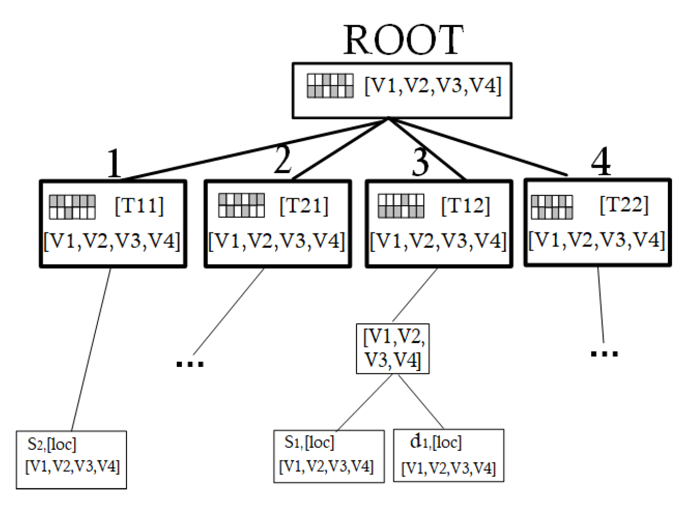
4.1.1. Building Hybrid Quad Tree

On the plain-text trajectory database, we build a hybrid quad tree base on quad tree [20] in $D{B}_p$. $D{B}_p$ includes all the points in $D{B}_{\tau }$ and $D{B}_o$. The space in a node is partitioned into four equal subspaces. The subspace is stored in the child node. The partitioning will not be stopped until there are less than n points in the subspace. First, the partitioning is based on $D{B}_{\tau }$, it will not be stopped until there are less than $N_{\tau }$ points in the subspace. The quad tree in this phase is called the father tree. The trajectory points are stored in every leaf node of the father tree. Then, every subspace in the leaf node of the father tree is partitioned. The partitioning is based on all points in this subspace; it will not be stopped until there is less than $N_o$ points in one leaf node. The quad tree takes the leaf node of the father tree, as its root node is called the child tree. Figure 4 shows the structure of a hybrid quad tree. The bold tree is the father tree. The others are child trees. Every non-leaf node of the hybrid quad tree stores the location vectors of four vertexes. Every leaf node stores the identities and location vectors of points in this leaf node. This is shown in line 1 of Algorithm 1.

4.1.2. Generating Filter Points and Pruning Transitions

If a reverse trajectory search is needed, we find the NN trajectory points for every query trajectory point and construct a table. In Figure 5, the NN points of query points ($q_1,q_2,q_3$) are in $node\left(1\right)$, $node\left(2\right)$, $node\left(3\right)$ and $node\left(4\right)$. Then, we find the trajectory, which has more than two points in the table, such as $T1$. All points in these trajectories are called filter points. In Figure 6, the filter points are $T11$ and $T12$. We form a polyline based on perpendicular bisectors between the points from one trajectory and the query points. The polyline divides the space into two subspaces. If one node is intersected by the polyline, then we check whether the child node meets the above condition. Then, $node\left(1\right)$ and the $node\left(3\right)$ are intersected by the polyline in Figure 5. Its child node needs to be checked. If the node is the leaf node of the child tree, we list all the transitions’ identity and compute the distance between the transition points and the filter points. If there are more than k trajectories closer to the transition than the query trajectory, the transition is pruned. In Figure 6, leaf $node(3,2,3)$ is intersected by the polyline, and we compare the distance $dist(O_2,Q)$ with the distance $dist(O_2,T1)$. Since $dist(O_2,Q)>dist(O_2,T1)$, transition $O_2$ can be pruned. If one node is in the subspaces of two filter points with one trajectory identity, the node is closer to the trajectory than the query trajectory. If there are more than k polylines that make one node meet the above condition, there are more than k trajectories closer to the node than to the query trajectory. All transitions in these nodes are closer to the k trajectories than to the query trajectory. All transitions in these nodes can be pruned. In Figure 5, the $node(3,1)$ is in the subspace of $T11$ and $T12$, all points in $node(3,1)$ are closer to trajectory $T1$ than to query trajectory Q. Since transition $O_1=(s_1,d_1)$ is in $node(3,1)$, it can be pruned. All the rest of the transitions are called candidate transitions. The candidate transitions in Figure 5 are $O_0$ and $O_3$.

4.1.3. Refining Transitions and Returning Results

For every candidate transition, we compute the distance between every point in transition and the query trajectory. We check the nodes in the quad tree by using a circle, of which the radius is the distance and the center point is the transition point. For the nodes in the circles of one transition, we record the identities of trajectories in these nodes. For the nodes that intersect with the circle, the child node needs to be checked further. If the node is a leaf node, we compute the distance between every transition point and trajectory in the leaf node. We record the identities of trajectories which are closer to the transition than the query trajectory. If the total number of recorded identities is more than k, then the candidate transition is deleted. In Figure 6, the circles of point $s_3$ and $d_3$ are drawn. The nodes $(2,1,4)$ and $(4,4,1)$ are in the circle, respectively. The trajectory $T2$ is closer to the transition $O_3$. It can be deleted in the candidate transitions. The rest of the candidate transitions are called refined transitions. For every point of the refined transitions, we find the NN points in the quad tree and check whether there are two points of query trajectory in it. If two points of the query trajectory are in the NN points of one transition, it is inserted in the set $RkNN\left(Q\right)$. The $RkNN\left(Q\right)$ is the search results. In Figure 5, the NN point for the point $s_0$ is $q_2$ and the NN point for the point $d_0$ is $q_3$. The $RkNNT\left(Q\right)$ in Figure 5 is $O_1$.

4.2. Reverse Search on Encrypted Trajectory Database

In this section, the points of transitions and trajectories are encrypted, and the hybrid quad tree is replaced by an encrypted RBF tree (eRBFtree) and the distance list (DList). This section is consists of four phases: setup, eRBFtree building, query encryption and search.

4.2.1. Setup

The data owner generates the parameters of CKKS and RBF tree as shown in Section 3.2. It encrypted all the location vectors of points in database $D{B}_p$. For a point with identity $ID$ and location $loc$, its item is $\{ID,CKK{S}_{enc}\left(loc\right)\}$. The $clou{d}_2$ generates its private key $s{k}_2$ and public key $p{k}_2$; it publishes the public key $p{k}_2$ to the DO and DU.

4.2.2. eRBFtree and DList Building

As shown in Figure 7, building an eRBFtree includes two steps. The first step is building the RBF tree in the database $D{B}_{\tau }$ and the partitioning of space is the same to the partitioning of the father tree in Section 4.1.1. Every leaf node of the RBF tree stores the encrypted items of trajectory points. Every non-leaf node stores an RBF and four encrypted points $\{CKK{S}_{enc}\left(V_1\right),\cdots ,CKK{S}_{enc}\left(V_4\right)\}$, where $V_i,i\in (1,4)$ is the four vertices of the node. The second step is building the child trees in the database $D{B}_o$. Every leaf node of the child tree stores encrypted items of transition points. Every non-leaf node stores four encrypted points $\{CKK{S}_{enc}\left(V_1\right),\cdots ,CKK{S}_{enc}\left(V_4\right)\}$. The DList is a table, in which every row records $(I{D}_o,p):\{di{s}_1,SI{D}_{\tau }^1\},\{di{s}_2,SI{D}_{\tau }^2\},\cdots$. The keywords $(I{D}_o,p)$ are the identity of transition and one point in the transition. The value $di{s}_i$ is the maximum distance from the point p to its nearby nodes. The value $SI{D}_{\tau }^i$ is the set of trajectories’ identities in these nodes. The values are listed in increasing order by the $di{s}_i$. The eRBFtree and the DList are constructed by the data owner. The DO encrypts the eRBFtree with all the items by the public key $p{k}_2$ and sends the cipher text to $clou{d}_2$. The DO sends the DList and the secret key of CKKS to $clou{d}_1$.

4.2.3. Query Encryption

The query includes tokens and items for points $q_j,j\in (1,N_p)$ in the query trajectory. $N_P$ is the number of points in the query trajectory. The token $Token\left(q_j\right)$ is for a secure kNN search in eRBFtree, which is constructed as shown in Section 3.2.2. The center point is the point of the query trajectory, and the search radius is set by the DO. The item $\left\{CKK{S}_{enc}\left(q_j\right)\right\}$ is the encrypted location vector of the point $q_j$. The query $Q=\{(Token\left(q_1\right),CKK{S}_{enc}\left(q_1\right)),\cdots ,\left(Token\right(q_{N_p}),$ $CKK{S}_{enc}\left(q_{N_p}\right)\left)\right\}$ is encrypted by the public key of $clou{d}_2$; then, it is sent to $clou{d}_2$ to start a reverse search.

4.2.4. Search

In this phase, $clou{d}_2$ decrypts the query with the private key $s{k}_2$. Then, $clou{d}_2$ uses the tokens $Token\left(q_j\right),j\in (1,N_p)$ to search the eRBF tree, obtains the NN trajectory points for every point in the query trajectory, checks the identities of points and constructs the filter set. The item in the filter set is $\{I{D}_{\tau },CKK{S}_{enc}\left(lo{c}_1\right),CKK{S}_{enc}\left(lo{c}_2\right),\cdots ,CKK{S}_{enc}\left(lo{c}_{N_p}\right)\}$, where $CKK{S}_{enc}\left(lo{c}_1\right),CKK{S}_{enc}\left(lo{c}_2\right),\cdots ,CKK{S}_{enc}\left(lo{c}_{N_p}\right)$ are NN points of $N_p$ query points. They have the same trajectory identity $I{D}_{\tau }$. $Clou{d}_2$ computes distances between every vertex in the node and the filter points by $DI{S}_1=CKK{S}_{di{s}^2}(CKK{S}_{enc}\left(lo{c}_i\right),CKK{S}_{enc}\left(V_j\right)),i\in (1,2),j\in (1,4)$. Then, $clou{d}_2$ computes the distance between every vertex in the node and the query trajectory by $DI{S}_2=CKK{S}_{di{s}^2}(CKK{S}_{enc}\left(q_i\right),CKK{S}_{enc}\left(V_j\right)),i\in (1,N_p),j\in (1,4)$. Afterwards, $clou{d}_2$ sends $DI{S}_1,DI{S}_2$ to the $clou{d}_1$. $Clou{d}_1$ decrypts them and obtains the distance between every vertex and the filter points $dist(lo{c}_i,V_j),i\in (1,2),j\in (1,4)$ and the distance between every vertex in node and the query trajectory $dist(q_i,V_j),i\in (1,N_p),j\in (1,4)$. The process is from the root node to the leaf node, using the pruning transition in Section 4.1.2. If one node is filtered, $clou{d}_1$ notifies $clou{d}_2$. Then, $clou{d}_2$ stops computing the distance of its child node. If the node is a leaf node, $clou{d}_2$ and $clou{d}_1$ compute the distance between every transition point in the node and the query trajectory $dist(lo{c}_i,q_j),i\in (1,2),j\in (1,N_p)$. After filtering the transitions, $clou{d}_2$ cooperates with $clou{d}_1$ to compute the distance between the candidate transitions and the query trajectory. The identities of transitions and the cipher text of distance are sent to $clou{d}_1$. Then, $clou{d}_1$ decrypts the cipher text and obtains the distance $d=dist(lo{c}_i^{can},q_j),i\in (1,2),j\in (1,N_p)$. For every candidate point $lo{c}_i^{can},i\in (1,2)$ in one transition, $clou{d}_1$ refers to the DList, locates the row of keyword $lo{c}_i^{can}$ and finds the maximum values for $di{s}_{h_i}$ meet $di{s}_{h_i}\le min\{dist(lo{c}_i^{can},q_j),j\in (1,N_p)\}$. Then, $clou{d}_1$ counts the number of trajectories, of which two points come from two sets $SI{D}_{\tau }^{h_1}$ and $SI{D}_{\tau }^{h_2}$. If the number of the trajectories is more than k, the transition ($lo{c}_1^{can},lo{c}_2^{can}$) can be pruned. Then, $clou{d}_1$ sends the identities of refined transitions $S_{ref}$ to $clou{d}_2$. For every refined transition ($s,d$) with identity in $S_{ref}$, $clou{d}_2$ sends the identity and a distance $di{s}_{ref}=dist(s,Q)+dist(d,Q)$ to the DO. Then, $clou{d}_2$ sends the encrypted transition $(CKK{S}_{enc}\left(lo{c}_s\right),CKK{S}_{enc}\left(lo{c}_d\right))$ points to the DO. The tokens $Toke{n}_{ref}$ for every point in the refined transition are constructed after the DO obtains the request $\{I{D}_O,di{s}_{ref}\},I{D}_O\in S_{ref}$ from $clou{d}_1$ and decrypts $(CKK{S}_{enc}\left(lo{c}_s\right),CKK{S}_{enc}\left(lo{c}_d\right))$. The DO constructs two tokens for every transition, as shown in Section 3.2.2. The center points are the points of location $lo{c}_s$ and $lo{c}_d$, respectively. The radius is $di{s}_{ref}$. The DO sends the set of tokens $Toke{n}_{ref}$ to $clou{d}_2$. $Clou{d}_2$ searches the NN points and checks if there is less than k trajectories in the NN points. If there are, the transition is one of the reverse k transitions for the query trajectory. Otherwise, $clou{d}_2$ computes the distance between trajectories and transitions with the help of $clou{d}_1$. $Clou{d}_1$ compares the distance between the trajectory and transitions as wel as between the query trajectory and transitions. If more than k trajectories are closer to one transition, the transition is deleted. The rest of the refined transitions are the results. Then, $clou{d}_1$ returns the identities to the DU and $clou{d}_2$ returns the encrypted locations to the DU.

5. Theoretical Analysis

5.1. Correctness Analysis

In this section, we will discuss the returned results, which are all reverse transitions for the query trajectory. The discussion is divided into three steps.

(1) In the first step, we find the filter set $S_{\tau }$ and prune the $O=(s,d)\in D{B}_o$ so that $\exists {\mathcal{D}}_{\tau }=\{{\tau }_1,\cdots ,{\tau }_k\}$ such that $dist(s,{\tau }_i)<dist(s,Q)$ and $dist(d,{\tau }_i)<dist(d,Q)$, $i\in (1,\cdots ,k)$. According to Definition 4, the transition cannot be in RkNNT(Q). We call the transition that is not in RkNNT(Q) a negative transition and the transition that is in RkNNT(Q) a positive transition. In this step, we only prune a part of the negative transitions. There are also many negative transitions in set $S_{can}$.

(2) In the second step, we use the candidate set $S_{can}$ and DList to delete the $O=(s,d),s\in S_{can}$ or $d\in S_{can}$ so that there exists $\{di{s}_s<dist(s,Q),SI{D}_{\tau }^s\}$ in the row of point s, $\{di{s}_d<dist(d,Q),SI{D}_{\tau }^d\}$ in the row of point d and $SI{D}_{\tau }^s\cap SI{D}_{\tau }^d$ has more than k trajectory identities. It also means that $\exists {\mathcal{D}}_{{\tau }^{\prime }}=\{{\tau }_1^{\prime },\cdots ,{\tau }_k^{\prime }\}\subset (SI{D}_{\tau }^s\cap SI{D}_{\tau }^d)$ such that $dist(s,{\tau }_i)<dist(s,Q)$ and $dist(d,{\tau }_i)<dist(d,Q)$, $i\in (1^{\prime },\cdots ,k^{\prime })$. In this step, we also delete a part of negative transitions. It is unclear whether there are any negative transitions in set $S_{ref}$.

(3) In the third step, we know that if a transition takes the query trajectory as one of its kNN trajectories, the transition must be the RkNNT of the query trajectory. For every transition $O=(s,d)\in S_{ref}$, we find all trajectory points with distance to s or d less than $di{s}_{ref}=dist(s,Q)+dist(d,Q)$. If a trajectory $\tau$ has only a point with distance to s or d less than $di{s}_{ref}$, then $dist(s,\tau )+dist(d,\tau )>di{s}_{ref}$. If a trajectory $\tau$ has no point with distance to s or d less than $di{s}_{ref}$, then $dist(s,{\tau }^{\prime })+dist(d,{\tau }^{\prime })>2di{s}_{ref}$. So if only a trajectory has one point with distance to s less than $di{s}_{ref}$ and the other one point has distance to d less than $di{s}_{ref}$, it is possibly closer to the transition $O=(s,d)$ than the query trajectory Q. For every transition $O=(s,d)\in S_{ref}$, we list all NN trajectories ${\tau }_i$ meets $dist(s,{\tau }_i)+dist(d,{\tau }_i)\le 2di{s}_{ref}$ and check the size of ${\mathcal{D}}_{\tau }=\{{\tau }_1,\cdots ,{\tau }_j\}$ such that $dist(s,{\tau }_i)+dist(d,{\tau }_i)<dist(s,Q)+dist(d,Q)$, $i\in (1,\cdots ,j)$. If the size of ${\mathcal{D}}_{\tau }$ is not more than k, the transition must be the positive transitions; otherwise, the transition must be the negative transition.

5.2. Security Definitions and Analysis

The two-clouds model is honest-but-curious, and the RkNNToE is processed in two phases. The definition of leakage functions [21] of two phases and the formal proof are proposed. It shows that RkNNToE is secure in an honest-but-curious clouds model.

Definition 5.

In an honest-but-curious clouds model, there are two participants $\mathcal{C}i,i\in (1,2)$ in a protocol $\mathcal{P}$. For ${\mathcal{C}}_i$, $f_i$ and $O_i$ are the execution function and its output, while $vie{w}_i$ is the view during an execution of $\mathcal{P}$. The protocol $\mathcal{P}$ is secure against a probabilistic polynomial time (PPT) honest-but-curious adversary if there exist simulators ${\mathcal{S}}_1$ and ${\mathcal{S}}_2$ such that:

$$({\mathcal{S}}_1(f_1,{\mathcal{L}}_1),f_2)\equiv (vie{w}_1,O_2)$$

(2)

$$(f_1,{\mathcal{S}}_2(f_2,{\mathcal{L}}_2))\equiv (O_1,vie{w}_2)$$

(3)

where ≡ means computational indistinguishability.

${\mathcal{L}}_i^j$ is the leakage function of cloud $i\in (1,2)$ in phase $j\in \{setup,search\}$. Given a collection of points $D{B}_p$ from the DO and a query trajectory Q from the DU,

$${\mathcal{L}}_1^{setup}\left(D{B}_p\right)=\{DL,[\mathbb{EI},[id,p]]\}$$

$${\mathcal{L}}_2^{setup}\left(D{B}_p\right)=\{\mathbb{EI},{(OID,\left[loc\right])}_i,{(TID,\left[loc\right])}_j,|D{B}_p|,|D{B}_{\tau }|,|D{B}_O\left|\right\}$$

$${\mathcal{L}}_1^{search}(D{B}_p,Q)=\{\mathbb{D}\left(Q\right),DL,S_{can},S_{ref}\}$$

$${\mathcal{L}}_2^{search}(D{B}_p,Q)=\{Toke{n}_i,Toke{n}_j,|Q|,|S_{ref}|,|S_{can}|,\mathbb{S}\left(Q\right),\mathbb{A}(Q),{(OID,\left[loc\right])}_i,{(TID,[loc])}_j\},$$

where $DL$ is the distance list, $EI$ is the eRBF tree, $id$ is the identity of point p, $[·]$ is the cipher text of ·, $|·|$ is the size of ·, $OI{D}_i$ is the identity of transition i and $TI{D}_j$ is the identity of trajectory j.

Definition 6.

(Search Pattern $\mathbb{S}$) The search pattern leakage reveals whether the keywords in the token of every query point have appeared before.

Definition 7.

(Access Pattern $\mathbb{A}$) Given a search query Q, the access pattern is defined as the identifier of trajectory points in the nearest neighbor of query points.

Definition 8.

(Distance Pattern $\mathbb{D}$) Given a search query Q, $\mathbb{D}\left(Q\right)=dist(p_i,q_j),q_j\in Q,p_i\in S_{can}$. Informally, this part of leakage can be derived from the query, $\mathbb{D}$ leaks the distances between the points in candidate transitions and query points.

Theorem 1.

Under the permitted leakage functions ${\mathcal{L}}_1^{Setup}$, ${\mathcal{L}}_2^{Setup}$, ${\mathcal{L}}_1^{Search}$ and ${\mathcal{L}}_2^{Search}$, if CKKS and the FSknn [19] are secure in the two honest-but-curious clouds model, then $RkNNToE$ is secure in the two honest-but-curious clouds model.

Proof. 

We introduce the leakage function to Definition 5 and prove that for any PPT adversary, there exist simulators $S_1$ and $S_2$ such that:

$$({\mathcal{S}}_1(f_1,{\mathcal{L}}_1^{setup}),f_2)\equiv (vie{w}_1,O_2)$$

(4)

$$({\mathcal{S}}_1(f_1,{\mathcal{L}}_1^{search}),f_2)\equiv (vie{w}_1,O_2)$$

(5)

[Simulating Setup] Given ${\mathcal{L}}_1^{setup}\left(D{B}_p\right)=\{DL,[\mathbb{EI},[id,p]]\}$, ${\mathcal{S}}_1$ randomly generates a message as the plain text m and encrypts it by using a CPA-secure encryption to obtain $\left[m\right]$. ${\mathcal{S}}_1$ randomly generates the identity of trajectories and transitions. The number of these trajectories is the same as the one listed in $DL$. ${\mathcal{S}}_1$ randomly generates many increasing arrays to represent the distance between the transition points and vertices of each node. Since the PPT adversary does not know the real distribution of points, and the encryption in the above simulation is secure, a PPT adversary cannot distinguish between the simulated view and the real view.

[Simulating Search] Given ${\mathcal{L}}_1^{search}(D{B}_p,Q)=\{\mathbb{D}\left(Q\right),DL,S_{can},S_{ref}\}$, ${\mathcal{S}}_1$ knows the identities of transitions that are deleted in the phase of refining transitions $S_{del}=S_{can}-S_{ref}$. From $\mathbb{D}\left(Q\right)$, ${\mathcal{S}}_1$ knows the distance between the point in $S_{can}$ and query points. In the simulated $D{L}^{\prime }$, if a transition is in $S_{del}$, it must have kNN trajectories closer than the query. A PPT does not know the locations of every point; it only knows the distance and the identities of deleted transitions. It cannot distinguish between the simulated $D{L}^{\prime }$ and the real $DL$.

$$(f_1,{\mathcal{S}}_2(f_2,{\mathcal{L}}_2^{setup}))\equiv (O_1,vie{w}_2),$$

(6)

$$(f_1,{\mathcal{S}}_2(f_2,{\mathcal{L}}_2^{search}))\equiv (O_1,vie{w}_2)$$

(7)

[Simulating Setup] Given ${\mathcal{L}}_2^{setup}\left(D{B}_p\right)=\{\mathbb{EI},{(OID,\left[loc\right])}_i,{(TID,\left[loc\right])}_j$, $|D{B}_p|,$

$|D{B}_{\tau }|,|D{B}_O\left|\right\}$, ${\mathcal{S}}_2$ randomly chooses $|D{B}_p|$ points, encrypts points by CKKS to obtain ${\left[loc\right]}^{\prime }$ and assigns the identity to these points. Then, ${\mathcal{S}}_2$ constructs an eRBF tree ${\mathbb{EI}}^{\prime }$, which has the same structure with $\mathbb{EI}$. For each node, ${\mathcal{S}}_2$ randomly generates four vectors $V_1^{\prime },\cdots ,V_4^{\prime }$ and encrypts them by CKKS. ${\mathcal{S}}_2$ associates encrypts ${\left[loc\right]}^{\prime }$ with its corresponding $OID$ or $TID$ in $\mathbb{EI}$. According to secure analysis in [19], a PPT adversary cannot distinguish between the simulated view and the real view.

[Simulating Search] Given ${\mathcal{L}}_2^{search}(D{B}_p,Q)=\{Toke{n}_i,Toke{n}_j,\left|Q\right|,S_{can},S_{ref},$

$\mathbb{S}\left(Q\right),\mathbb{A}\left(Q\right),{(OID,\left[loc\right])}_i,{(TID,\left[loc\right])}_j\}$, ${\mathcal{S}}_2$ randomly generates plain text $lo{c}^{\prime }$ and encrypts it by using CKKS to get ${\left[loc\right]}^{\prime }$. From $\mathbb{S}\left(Q\right)$, ${\mathcal{S}}_2$ knows whether a point in query has been searched before or not. From $\mathbb{A}\left(Q\right)$, ${\mathcal{S}}_2$ knows the identifiers of points which are NN points for a query point. If a $q_i\in Q$ is searched before by comparing the token of $q_i$ and in previous tokens, ${\mathcal{S}}_2$ reuses the previous simulated token and returns the previous NN points as search results. Otherwise, ${\mathcal{S}}_2$ simulates a new search token $Toke{n}^{\prime }$, which is the token of one point including k hashes $h\left(kw\right)$ and a location. Since ${\mathcal{S}}_2$ knows which leaf node of the eRBF tree matches the search token $Toke{n}_j$, ${\mathcal{S}}_2$ randomly generates a k-bit string as the search token $Token$. The string has the same size as $h\left(kw\right)$ and matches with the same leaf node of eRBF. A PPT cannot distinguish between the simulated $Toke{n}^{\prime }$ and the real $Token$. □

5.3. Computational Complexity Analysis

In this section, we analyze the time complexity of RkNNToE, in which the most complexity is caused by computing the distance between two points securely. The complexity of kNN is shown in [19]. To generate the set $S_{can}$, every query point is checked against nodes and cost $\mathcal{O}\left(\right|Q|·(N_{vis}\left(eRBFtree\right)+N_{vis}\left(O_{leaf}\right)))$ at most, where $N_{vis}\left(eRBFtree\right)$ is the number of vertexes in the visited nodes and $N_{vis}\left(O_{leaf}\right)$ is the number of transition points in the leaf nodes that are intersected by the polyline. All filter points are checked against nodes and the cost of computing the distance is $\mathcal{O}(k·|Q|·(N_{vis}\left(eRBFtree\right)+N_{vis}\left(O_{leaf}\right)))$ at most. After obtaining $S_{can}$, the cost of computing the distances between all transitions in set $S_{can}$ and the query trajectory is $\mathcal{O}\left(\right|Q|·|S_{can}\left|\right)$. After obtaining $S_{ref}$, the cost of computing the distances between all transitions in set $S_{ref}$ and their kNN trajectories is $\mathcal{O}\left(2\right|S_{{\tau }^{\prime }}|·|S_{ref}\left|\right)$, where $S_{{\tau }^{\prime }}$ is a set of all kNN trajectories of a transition. The total complexity is $\mathcal{O}\left(RkNNToE\right)=\mathcal{O}((k+1)·|Q|·(N_{vis}\left(eRBFtree\right)+N_{vis}\left(O_{leaf}\right)))+\mathcal{O}(\left|Q\right|·|S_{can}\left|\right)+\mathcal{O}\left(2\right|S_{{\tau }^{\prime }}|·|S_{ref}\left|\right)$. According to [9], the visited nodes are proportional to the number of points in $D{B}_p$, f is the fanout of the eRBFtree, and $D{B}_{\tau }\ll D{B}_o$. The complexity is $\mathcal{O}\left(RkNNToE\right)=\mathcal{O}((k+1)·|Q|·(N_{vis}\left(eRBFtree\right)+N_{vis}\left(O_{leaf}\right)))+\mathcal{O}(\left|Q\right|·|S_{can}\left|\right)+\mathcal{O}\left(2\right|S_{{\tau }^{\prime }}|·|S_{ref}\left|\right)=\mathcal{O}((k+2)·\left|Q\right|·\left(\right|D{B}_o|/f))$.

6. Performance Evaluation

In this section, we conduct experiments on the two databases: the aGPS trajectory dataset (Transition dateset) collected in Geolife project in Beijing [22,23,24] and the bus lines dataset (Trajectory dataset) in Beijing [25]. There are 18,670 transitions in the transition database. The bus lines dataset has 1891 trajectories and 1174 bus stations. All algorithms are implemented in Python language in Windows 10 and examined on a computer with an Intel(R) Core (TM)i5-10505 and 16.00 GB RAM. We randomly generate a query trajectory by selecting an ordered sequence from the trajectory database, since the randomly generated points cannot keep the spatial continuity as a trajectory. In the experiment, the NN k trajectories do not share any one point with the query trajectory. The trajectory that is shared by multiple bus lines is just recorded as one trajectory.

6.1. Constructing eRBF Tree and DList

Before outsourcing the data, the DO needs to build the eRBF tree. The time cost of constructing the eRBF index includes two parts: the time of constructing the RBF tree in database $D_{\tau }$ and the time of constructing the encrypted quad tree in database $D_p$. The first part is related with the maximum number ($N_{\tau }$) of trajectory points in a leaf node of the father tree.

Table 3. The cost of constructing father tree and DList.

DB	${\mathit{N}}_{\mathit{\tau }}$	Step Length in Latitude and Longitude	Time Cost of RBF Tree(s)	Time Cost of DList(s)
$D{B}_{\tau }$	2	[0.000230, 0.001237]	5.600787	3.559773
	3	[0.000460, 0.002474]	3.796525	3.468612
	4	[0.001840, 0.009896]	2.861059	3.470150
	5	[0.001840, 0.009896]	2.698736	3.444898

shows the time cost of constructing the RBFs in the father tree with different $N_{\tau }$. The second part is related to the maximum number ($N_o$) of transition points in a leaf node of the child tree. The total time of constructing the eRBF tree is shown in Figure 8; the main cost is for encrypting the four vertexes in every node of eRBF tree. With $N_{\tau }$ or $N_o$ increasing, the cost of constructing eRBF decreases, since the DList is constructed based on plain text, and the DO only needs to compute the distance between every transition point with vertexes in its nearby nodes. Here, we set the nodes in the range of 25 to 200 steps, and the mean time of constructing the DList is shown in Table 3.

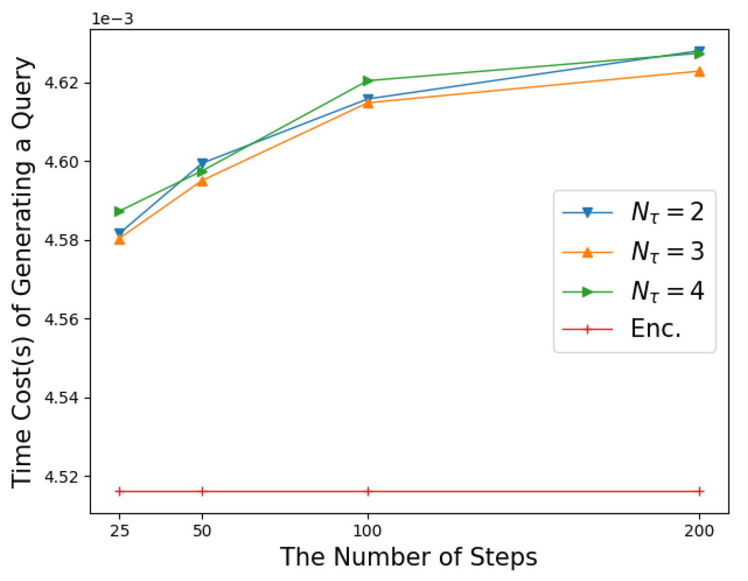
6.2. Generating Query

A query of one point includes the encrypted location and an NN search token. The time cost of encrypting a location vector is about 0.004516 seconds by CKKS encryption. The cost of generating a token is related with the search radius. Here, we denote the minimum range of the leaf node in the father tree as a step length and use the number of steps to determine the search radius. The step length does not decrease as $N_{\tau }$ increases, which is shown in Table 3. As shown in Figure 9, the line of “Enc.” is the time of encryption of a location. As the number of steps increases, the time of generating a token increases. So, the total time to generate a trajectory query is related to the number of points included in this trajectory and the search radius for every point in the query.

6.3. Search

In this section, we firstly demonstrate the time cost of the kNN search for a point. Then we show the total time of two clouds after receiving a RkNNToE request.

6.3.1. NN Trajectories Search

Since the DO needs to search NN trajectories for the refined transitions, it is necessary to illustrate the efficiency of the kNN search for every transition point. As shown in Figure 10, as the number of trajectory points in a leaf node of the father tree increases, the time of searching the NN points increases. As the number of steps in the search radius increases, the time cost of searching NN points increases. The total cost of searching NN trajectories for a transition requires twice as much time as that for NN points in Figure 10.

6.3.2. RkNNToE Search

In this section, we simulate the whole search process in two clouds, which includes finding NN points for every query point, constructing a filter set and pruning transitions, refining transitions and finding NN trajectories for every refined transition. In the simulated search, the eRBF tree is built with $N_{\tau }=2$ and $N_o=2$. The experiment settings are as follows:

The number of points in a query($N_p$): 2 to 5, default 3. The k in RkNNToE: 1 to 4, default 2. The number of steps in NN points search: 20 to 200.

The random behavior of a time cost is caused by the random generation query trajectory. The effect of pruning differs widely when the queries are different. According to Section 5.3, the complexity is mainly affected by $S_{can}$ and $(D{B}_O/f)$ rather than operations of search k $NN$ trajectories. $S_{can}$ and $(D{B}_O/f)$ are the outputs of pruning, and the size of the filter set does not linearly increase as k increases. In most cases, when $k=2$, the points in the filter set are $a,b,c$. $\{a,c\}$ and $\{a,b\}$ can form two trajectories. It also causes the random behavior of time cost. So, we use the median of time cost to analyze the distribution trend of the results. As shown in Figure 11, when the number of points in a query is 3, the median time cost decreases as k increases. As k increases, the number of trajectories in the filter set increases, and the filtered transition increases. In the refining phase, the number of candidate transitions decreases, which leads to the reduction of time. As shown in Figure 12, when $k=2$, the median of the time cost is increased as the number of points in a query increases. As the number of points in a query increases, the number of points in the trajectories in the filter set increases, which leads to the increased times of computing distance. It also results in the decrease of pruning space, which means the number of refined transitions increases. Both conditions cause the cost time to increase.

7. Conclusions

In this paper, we studied a method of route planning on an encrypted trajectory database, RkNNToE, that securely returns all transitions, which are the reverse k nearest neighbor trajectories of the query trajectory. We designed a hybrid encrypted bloom filter tree (eRBFtree) for search in the encrypted trajectory database, which supports space pruning and fast kNN search. Combined with eRBFtree, we gave the pruning strategies to prune the transition as much as possible and to improve the search efficiency. The security analysis showed that the query, data and index are secure in the process of RkNNToE. The experiments showed that RkNNToE can find the results in the RkNNT search efficiently and correctly.

References

1. Chen, Z.; Shen, H.T.; Zhou, X.; Zheng, Y.; Xie, X. Searching trajectories by locations: An efficiency study. In Proceedings of the ACM SIGMOD International Conference on Management of Data, Indianapolis, IN, USA, 6–10 June 2010; pp. 255–266. [Google Scholar] [CrossRef]
2. Keogh, E.J. Exact indexing of dynamic time warping. In Proceedings of the VLDB, Hong Kong, China, 20–23 August 2002; pp. 406–417. [Google Scholar]
3. Vlachos, M.; Gunopulos, D.; Kollios, G. Discovering similar mul- tidimensional trajectories. In Proceedings of the ICDE, San Jose, CA, USA, 26 February–1 March 2002; pp. 673–684. [Google Scholar]
4. Chen, L.; Özsu, M.T.; Oria, V. Robust and fast similarity search for moving object trajectories. In Proceedings of the SIGMOD, Baltimore, MD, USA, 14–16 June 2005; pp. 491–502. [Google Scholar]
5. Cheema, M.A.; Zhang, W.; Lin, X.; Zhang, Y.; Li, X. Continuous reverse k nearest neighbors queries in Euclidean space and in spatial networks. VLDB J. 2012, 21, 69–95. [Google Scholar] [CrossRef]
6. Emrich, T.; Kriegel, H.P.; Mamoulis, N.; Niedermayer, J.; Renz, M.; Zufle, A. Reverse-nearest neighbor queries on uncertain moving object trajectories. In Database Systems for Advanced Applications; Springer: Berlin/Heidelberg, Germany, 2014; pp. 92–107. [Google Scholar]
7. Feng, Z.; Zhu, Y. A Survey on Trajectory Data Mining: Techniques and Applications. IEEE Access 2017, 4, 2056–2067. [Google Scholar] [CrossRef]
8. Zheng, Y.; Lu, R.; Zhu, H.; Zhang, S.; Guan, Y.; Shao, J.; Wang, F.; Li, H. SetRkNN: Efficient and Privacy-Preserving Set Reverse kNN Query in Cloud. IEEE Trans. Inf. Forensics Secur. 2023, 18, 888–903. [Google Scholar] [CrossRef]
9. Wang, S.; Bao, Z.; Culpepper, J.S.; Sellis, T.; Cong, G. Reverse k nearest neighbor serach over trajectories. IEEE Trans. Knowl. Data Eng. 2018, 30, 757–771. [Google Scholar] [CrossRef] [Green Version]
10. Pan, X.; Nie, S.; Hu, H.; Yu, P.S.; Guo, J. Reverse Nearest Neighbor Search in Semantic Trajectories for Location-Based Services. IEEE Trans. Serv. Comput. 2022, 15, 986–999. [Google Scholar] [CrossRef]
11. Tzouramanis, T.; Manolopoulos, Y. Secure reverse k-nearest neighbors search over encrypted multi-dimensional databases. In Proceedings of the 22nd International Database Engineering & Applications Symposium (IDEAS), Villa San Giovanni, Italy, 18–20 June 2018; pp. 84–94. [Google Scholar]
12. Tao, Y.; Papadias, D.; Lian, X. Reverse kNN search in arbitrary dimensionality. In Proceedings of the 30th International Conference Very Large Data Bases, Toronto, ON, Canada, 31 August–3 September 2004; pp. 744–755. [Google Scholar]
13. Wu, W.; Yang, F.; Chan, C.-Y.; Tan, K.-L. FINCH: Evaluating reverse k-nearest-neighbor queries on location data. Proc. Vldb Endow. 2008, 1, 1056–1067. [Google Scholar] [CrossRef]
14. Lu, J.; Lu, Y.; Cong, G. Reverse spatial and textual k nearest neighbor search. In Proceedings of the ACM SIGMOD International Conference on Management Data, Athens, Greece, 12–16 June 2011; pp. 349–360. [Google Scholar]
15. Lu, Y.; Cong, G.; Lu, J.; Shahabi, C. Efficient algorithms for answering reverse spatialkeword nearest neighbor queries. In Proceedings of the 23rd SIGSPATIAL International Conference on Advances in Geographic Information Systems, Bellevue, WA, USA, 3–6 November 2015; pp. 1–4. [Google Scholar]
16. Pournajaf, L.; Tahmasebian, F.; Xiong, L.; Sunderam, V.; Shahabi, C. Privacy preserving reverse k-nearest neighbor queries. In Proceedings of the 19th IEEE International Conference Mobile Data Manage, (MDM), Aalborg, Denmark, 25–28 June 2018; pp. 177–186. [Google Scholar]
17. Li, X.; Xiang, T.; Guo, S.; Li, H.; Mu, Y. Privacy-preserving reverse nearest neighbor query over encrypted spatial data. IEEE Trans. Serv. Comput. 2022, 15, 2954–2968. [Google Scholar] [CrossRef]
18. Wang, Q.; He, M.; Du, M.; Chow, S.S.; Lai, R.W.; Zou, Q. Searchable encryption over feature-rich data. IEEE Trans. Dependable Secur. Comput. 2016, 15, 496–510. [Google Scholar] [CrossRef]
19. Lei, X.; Tu, G.H.; Xie, A.X.L.T. Fast and Secure kNN Query Processing in Cloud Computing. In Proceedings of the 2020 IEEE Conference on Communications and Network Security (CNS), Avignon, France, 29 June–1 July 2020. [Google Scholar]
20. Finkel, R.A.; Bentley, J.L. Quad trees a data structure for retrieval on composite keys. Acta Inform. 1974, 4, 1–9. [Google Scholar] [CrossRef]
21. Lindell, Y. How to simulate it—A tutorial on the simulation proof technique. In Tutorials on the Foundations of Cryptography; Springer: Berlin/Heidelberg, Germany, 2017; pp. 277–346. [Google Scholar]
22. Zheng, Y.; Zhang, L.; Xie, X.; Ma, W. Mining interesting locations and travel sequences from GPS trajectories. In Proceedings of the International conference on World Wild Web (WWW 2009), Madrid, Spain, 20–24 April 2009; ACM Press: New York, NY, USA, 2009; pp. 791–800. [Google Scholar]
23. Zheng, Y.; Li, Q.; Chen, Y.; Xie, X.; Ma, W. Understanding Mobility Based on GPS Data. In Proceedings of the ACM conference on Ubiquitous Computing (UbiComp 2008), Seoul, Republic of Korea, 21–24 September 2008; ACM Press: New York, NY, USA, 2008; pp. 312–321. [Google Scholar]
24. Zheng, Y.; Xie, X.; Ma, W. GeoLife: A Collaborative Social Networking Service among User, location and trajectory. IEEE Data Eng. Bull. 2010, 33, 32–40. [Google Scholar]
25. BeiJIngBusStation. Available online: https://github.com/FFGF/BeiJIngBusStation (accessed on 7 March 2023).
Figure 1. Inserting a keyword on an empty RBF.
Mathematics 11 01546 g001
Figure 2. Index structure: RBF tree.
Mathematics 11 01546 g002
Figure 3. The model of RkNNToE search.
Mathematics 11 01546 g003
Figure 4. The partition for all points.
Mathematics 11 01546 g004
Figure 5. The quad tree structure for all points.
Mathematics 11 01546 g005
Figure 6. The example of RkNN search.
Mathematics 11 01546 g006
Figure 7. The structure of eRBFtree. [ · ] is the encryption of ·.
Mathematics 11 01546 g007
Figure 8. The time cost of constructing the eRBF tree.
Mathematics 11 01546 g008
Figure 9. The time cost of generating a query.
Mathematics 11 01546 g009
Figure 10. The time cost of searching NN trajectory points.
Mathematics 11 01546 g010
Figure 11. The effect of k in RkNNToE search ( N P = 3 ).
Mathematics 11 01546 g011
Figure 12. The effect of the number of points in query ( k = 2 ).
Mathematics 11 01546 g012