

CNN and Bidirectional GRU-Based Heartbeat Sound Classification Architecture for Elderly People
 , ,
, ,  , , , ,
Abstract
:1. Introduction
1.1. Research Contributions
- To propose a novel attention-based CNN + BiGRU architecture for abnormal heartbeat audio classification;
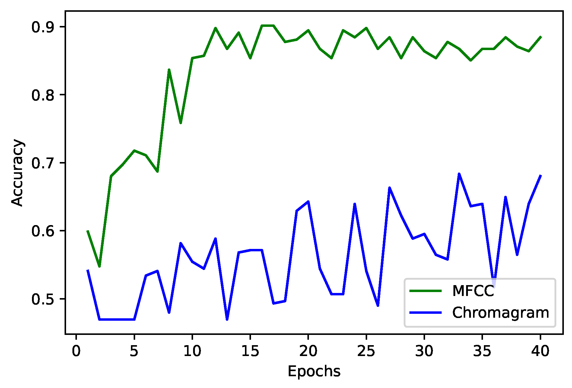
- To employ Mel-frequency cepstral coefficient (MFCC) for feature extraction, data compression, and downsampling as a pre-processing step to train the AI models efficiently;
- To evaluate the proposed architecture using different evaluation metrics, like statistical measures such as accuracy, precision, recall, etc., validation accuracy with and without data augmentation, and validation accuracy with different optimizers.
1.2. Organization
2. Related Work

| Related Works | Year | Key Contributions | Technology Used | Merits | Demerits |
|---|---|---|---|---|---|
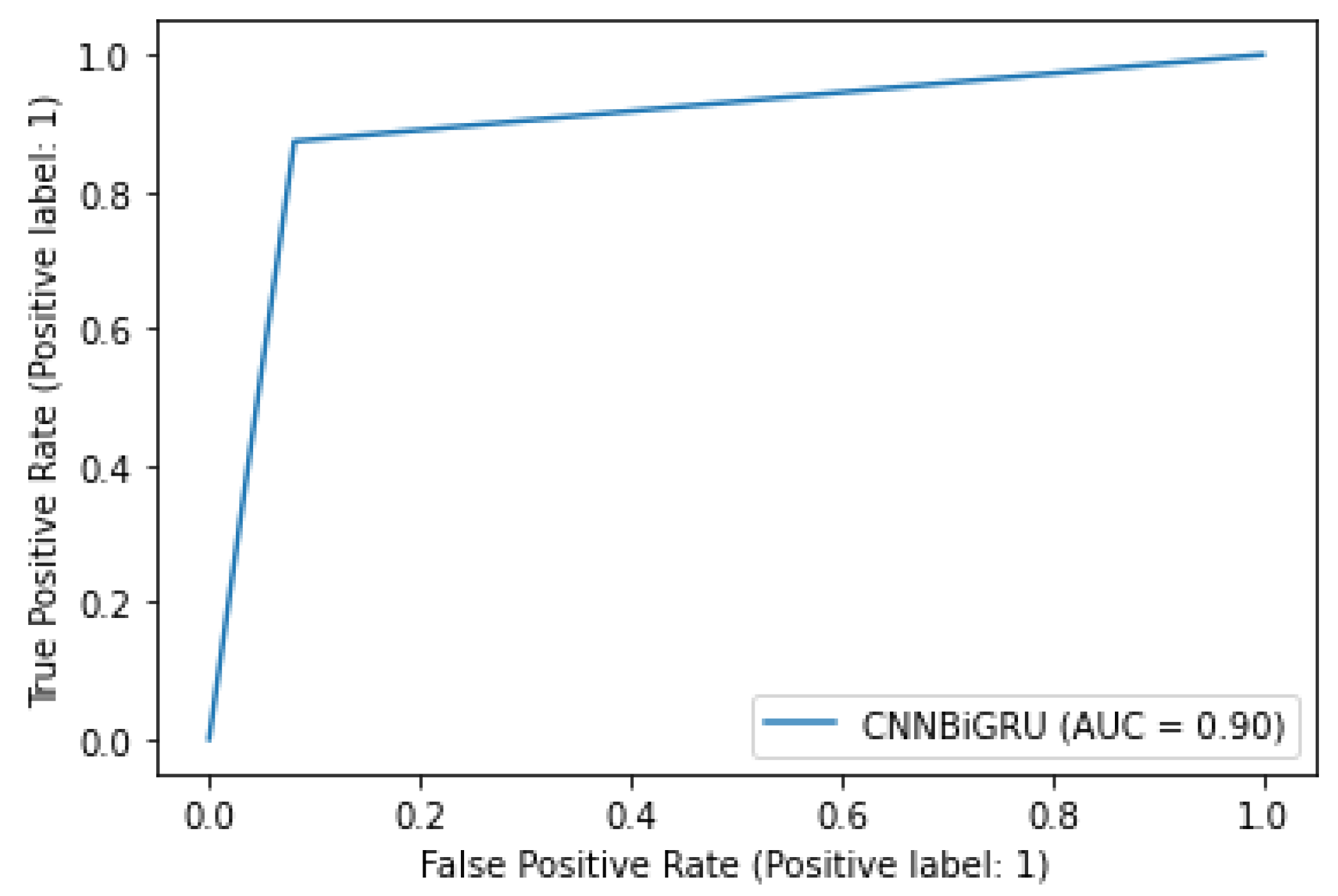
| Proposed Architecture | 2023 | To propose a model to perform heart sound classification on the CirCor DigiScope dataset | CNN+BiGRU and attention | 90% accuracy on the testing dataset and performed data augmentation as well | – |
| [23] | 2023 | Executed heart sound classification using two-dimensional features | Different ML, DL, and TL models | Used a wide range of models and feature extraction techniques to get better results | MFCC could have been used to further improve the results |
| [24] | 2023 | Heartbeat sound classification using a swarm intelligence-based algorithm | ABC-ANFIS | Used a novel approach of artificial bee colony along with ANFIS | The ABC-ANFIS method is quite complex |
| [29] | 2022 | A lightweight and robust approach for the detection of automatic heart murmurs using PCG recordings | Lightweight CNN | Uses two data augmentation techniques with low training and inference time | Accuracy of 75.1% is quite low compared to other models with similar architectures |
| [25] | 2022 | To detect a murmur in heartbeat sounds using a self-supervised approach | Self-supervised CNN backbone | Self-supervised model employed along with different data augmentation techniques | The accuracy of 73.7% is quite low and can be improved significantly |
| [26] | 2022 | To use XAI in heartbeat sounds with deep attention-based neural networks | CNN + attention and LSTM/GRU + attention | Used attention-based mechanism and validated results using XAI | Data augmentation does not improve the model results and does not tackle overfitting |
| [28] | 2022 | To classify lung and heartbeat sounds using feature-based fusion models | Fusion of CNNs | Applied learning in the form of fusion models and achieved an accuracy of 97% in six classes with data augmentation | Does not address overfitting concerns with a very small dataset for six classes and the degree of class imbalance is not explained |
| [30] | 2021 | To propose a model identifying abnormalities in a human heart using heart sound analysis | Artificial neural network (ANN) and linear discriminant analysis (LDA) | Achieved 90%, 83.33%, and 93.33% accuracy in the time, frequency, and time-frequency domain, respectively | Integration with DL algorithms might result in more accuracy |
| [20] | 2021 | To propose a model for the classification of heartbeat sound using mel-frequency spectral coefficients (MFSC) | CNN and hidden Markov model (HMM) | 86.25% accuracy for multi-classification achieved | Poor performance of the test set |
| [31] | 2021 | To use MFSC and deep residual learning for reducing the cost and time of hearbeat sound classification | One-dimensional local binary pattern (1D-LBP) and local ternary pattern (1D-LTP), and 1D-CNN | Accuracy of 91.78% and 91.66% achieved with PhysioNet and PASCAL dataset | Use of SVM on these datasets works better |
| [19] | 2021 | To propose a model that converts heart sound to visual scale spectrograms | CNN, ResNet152V2, MobileNetV2 | To extract features and categorize heart sounds using a TL approach | The time and pitch shift in audio was not tested |
| [18] | 2021 | To propose a model heart sound classification in HSS corpus using a Hamming window | CNN, GRU-recurrent neural network (RNN), and LSTM-RNN | Average recall of 51.2% achieved | Data size limitation |
| [32] | 2020 | To propose a 1D-CNN architecture for heart sound classification | CNN | Used stacked transition and clique blocks for promising classification performance, with lower consumption of parameters, and discriminative features extracted | Environment noises are not considered |
| [33] | 2020 | To propose a model for heartbeat sound classification using PCG signals to identify irregularities and achieving good cardiac diagnosis | CNN | Discrete cosine transform (DCT) achieved classification accuracy | A large number of samples are not taken for experiments |
3. Problem Formulation
4. Proposed Architecture
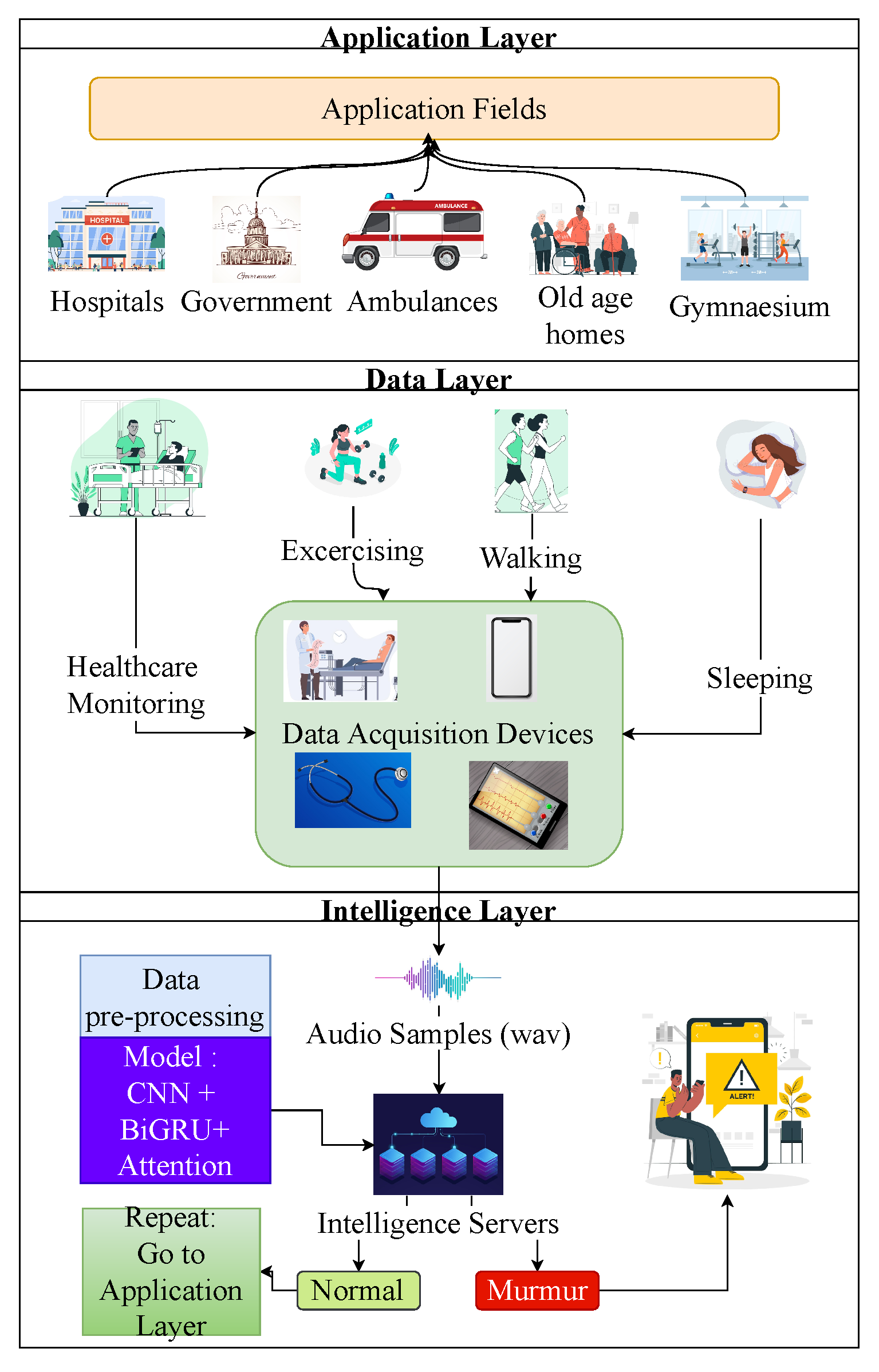
4.1. Application Layer
4.2. Data Layer
4.2.1. Dataset Description
4.2.2. Data Augmentation
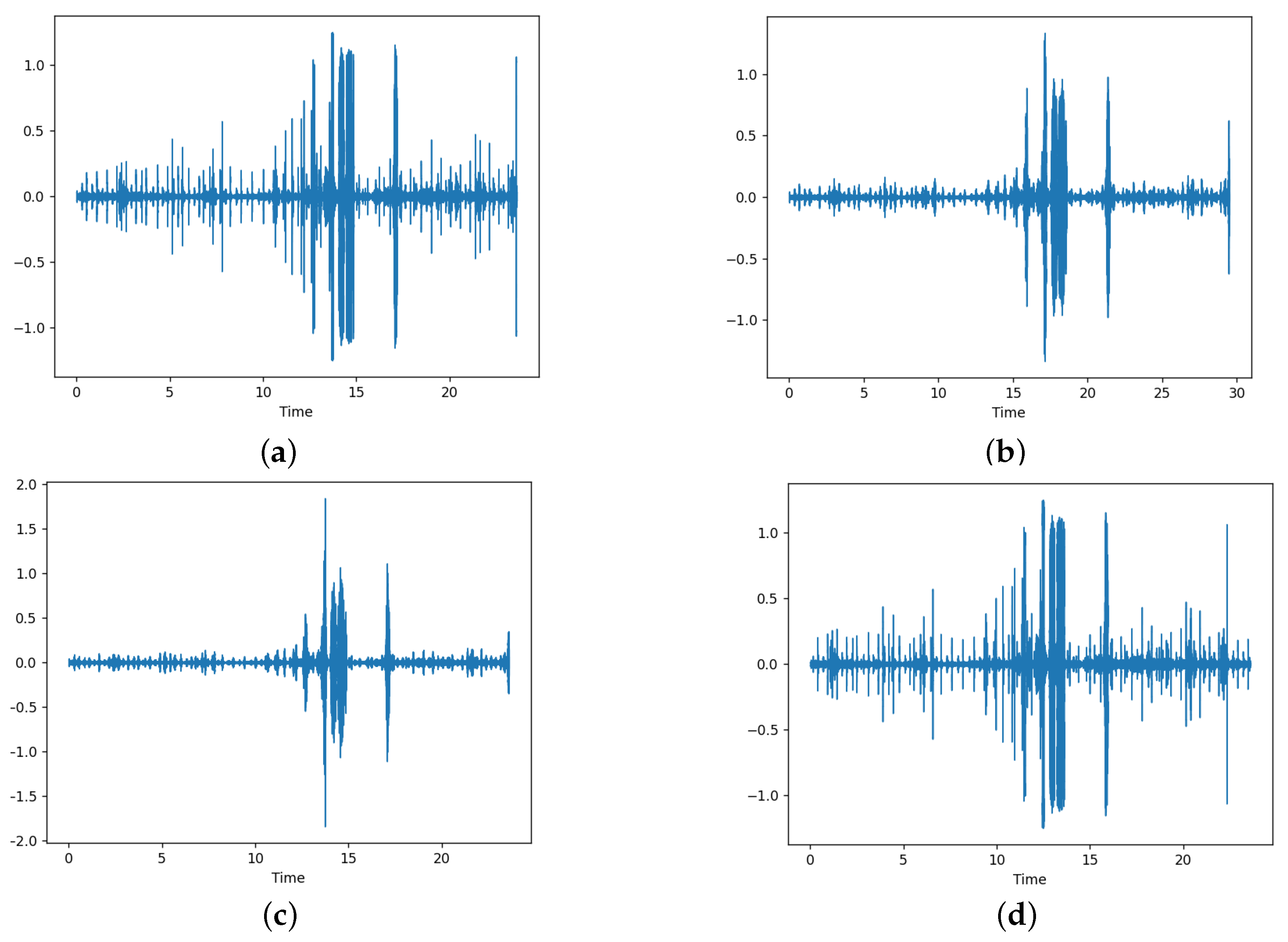
- Time stretch—this transformation is used to change the duration or speed of the signal without altering the original pitch. We can change the audio by speeding up the audio signal or slowing it down. If the selected rate is less than 1, the audio is slowed down and if it is greater than 1, it is sped up. We have used the librosa library for applying this transformation with the rate selection done uniformly between 0.8 and 1.2. We have set the probability of application of this transformation to 0.5, which means that the transformation is only applied with half the probability. Figure 2a,b shows the effects of time stretch.
- Pitch shift—this transformation is used to change the pitch or perform pitch shift by changing the sound pitch up or down without altering the tempo. We can change the audio signal by changing the pitch by reducing or increasing the semitones. We randomly select the semitones in the range of −4 to +4. Again, we set the probability of application of this transformation to 0.5, which means that the transformation is only applied with half the probability. Figure 2a,c shows the effects of pitch shift.
- Audio shift—this transformation is applied to shift the audio samples forward or backward, with or without any rollover. The shifting is done within a fraction of −0.5 to +0.5 of the audio signal. Furthermore, we set the probability of application of this transformation to 0.5, which means that the transformation is only applied with half the probability. Figure 2a,d shows the effects of audio shifting. As shown by comparison, the audio is the same but it is shifted by some amount.
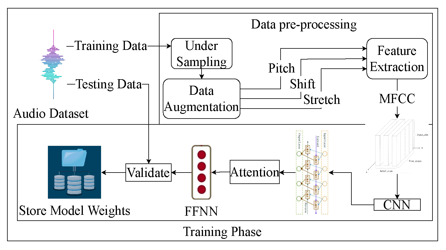
4.2.3. Data Pre-Processing
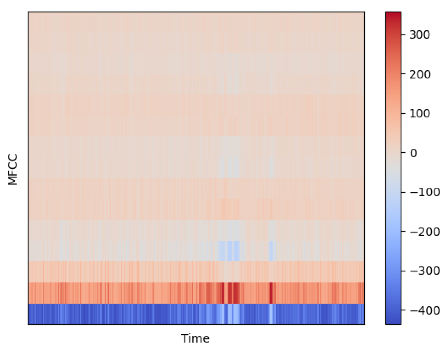
4.2.4. Feature Extraction
- Divide the raw audio into a set of frames ().
- Take the Fourier transform or fast Fourier transform (FFT) of the signal to get the power spectrogram for each frame.where represents the power spectrum of frame f.
- Map power of spectrum onto the Mel scale with the use of triangular overlapping windows. Mapping onto the Mel scale is represented below.where MSf represents the Mel scale values for each frame.
- Calculate logs of powers for each Mel frequency.where represents the power of the Mel frequencies and LMSf represents the log of the corresponding Mel scale values.
- Derive discrete cosine transform (DCT) of the list of Mel log powers.where MFCCf represents the MFCCs obtained for a frame of an audio file.
4.3. Intelligence Layer
- 2D convolution layer—After adding the bias to an intermediate convolved output, a 2D convolution layer convolves over an input image to produce an output. This creates an output image obtained by the convolution of a learnable kernel matrix on the input image. This is similar to a dense layer but is done on 2D images and has the advantage of parameter sharing. The equation below represents this operation,where represents the output image, represents the input image, represents the weight matrix (kernel), represents the activation function, ⨂ represents the convolution operation, and b represents the bias.
- Batch normalization layer—the batch normalization layer is used to normalize the inputs in the input layer such that the output standard deviation is close to 1. In contrast, the mean of the output is maintained to be close to 0. This layer scales the input by a learnable scale factor and offsets it by a learnable offset. This layer is generally used between the neural and output activation functions. This layer helps reduce the network’s sensitivity and speeds up the training speed.
- Dropout layer—the dropout layer is used to counter overfitting. This layer drops or makes the input units null and void in the network by a certain probability p set as a hyperparameter. The dropped units do not participate in the network’s forward and backward propagation during the current iteration. This helps in reducing overfitting because the model has exponentially many network architectures to train within the same network. After all, which unit is dropped at each iteration is not fixed. At the time of inference, however, the unit’s outputs are multiplied by the same probability p for forward propagation to represent that unit’s contribution to inferencing.
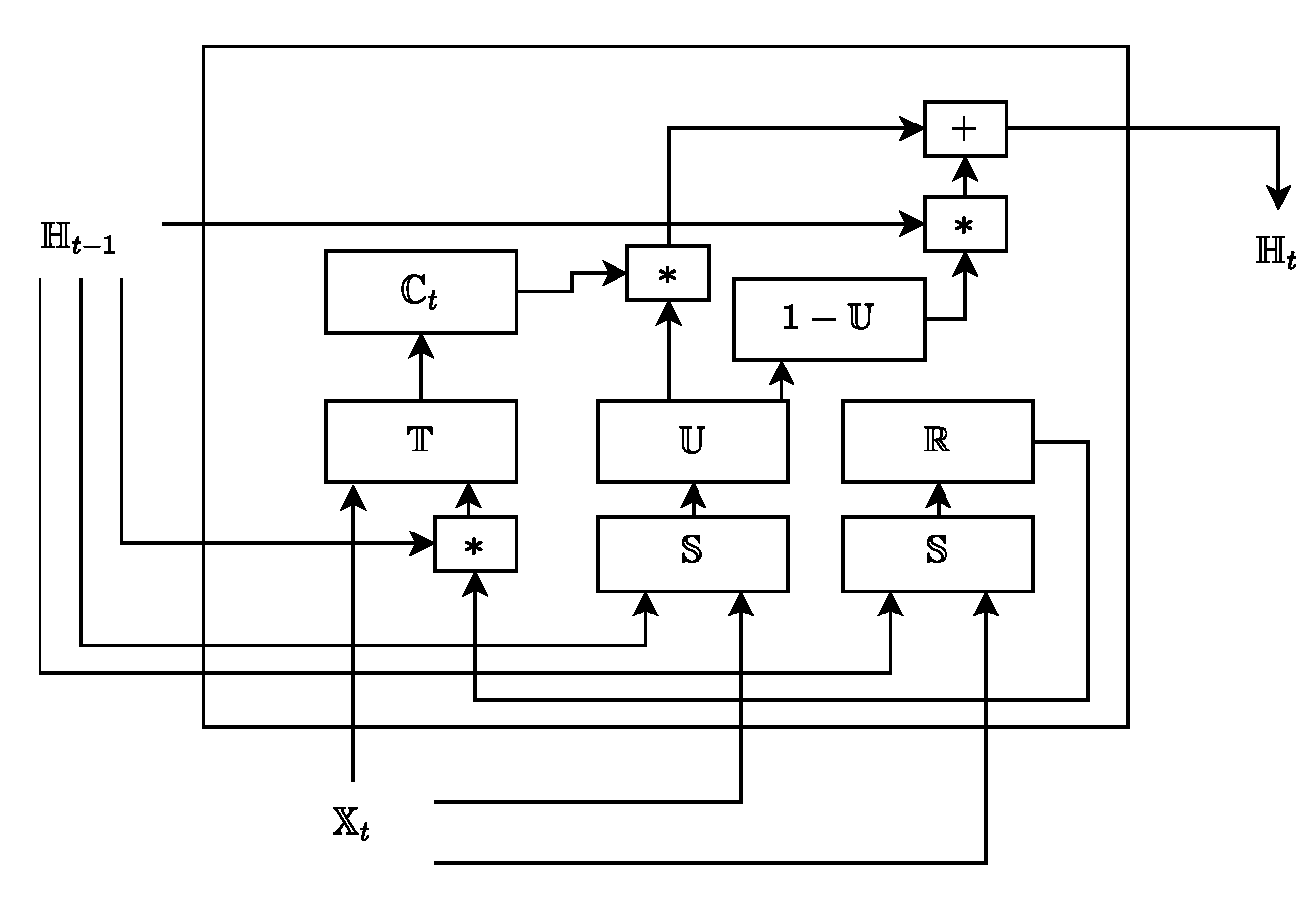
- GRU—they continually capture long-term dependencies in data using memory blocks. Each memory block has two gates, the update, and the reset gate, for performing the operations of updating the current memory cell state and deciding the amount of previous information to forget, respectively. The equations followed by a GRU unit are as follows.where the update gate is denoted as and the reset gate is denoted with , respectively. Further, the hidden state is denoted with for a timestamp t, means cell state for time t, and input features are denoted with , which are fed to the cell. , , , , , are the weights, and , , are the biases, which are obtained from the backpropagation algorithm (equipped in the neural network). × represents matrix multiplication and ∗ denotes element-wise dot product. is the tanh and is the sigmoid activation functions to show the probability of the neuron being active or inactive, respectively. Figure 5 represents the GRU unit.
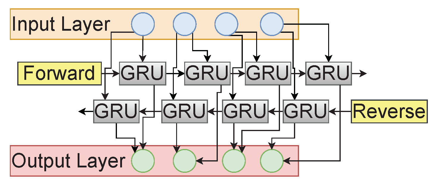
- Bidirectional GRU—GRUs help address the problem of vanishing and exploding gradient present in the case of RNN and help retain long-term information from past time steps. Bi-GRU is the extension of GRU that works in both directions, incorporating past and future time steps. Bi-GRU is composed of two GRU layers propagating in forward and backward directions. This helps us achieve improved performance in sequential decision-making problems by utilizing the complete context of the problem. Figure 6 illustrates the Bi-GRU’s structure.The BiGRU structure can be individually broken down into two different layers, i.e., the forward propagation layer and the backward propagation layer. Both layers differ only in the direction of the context they witness before making a prediction. The forward layer predicts a timestep considering the context before that timestep, i.e., the previous context. In contrast, the backward layer predicts a timestep considering only the context that occurs after that timestep i.e., future context. Hence, at any timestep, we have both the past and future context; consequently, the model makes better predictions. As seen in Figure 6, the GRU unit used in each layer is the same as in Equation (18). Now, let us consider the hidden output at any timestep ‘t’ for the forward layer’s GRU unit and the corresponding backward layer’s GRU unit to be and , respectively. The output at the timestep, say , can be given as follows.where , , and represent the weight matrix between the forward layer and output, the weight matrix between the backward layer, and bias for the output layer, respectively. represents the tanh activation function.
- Attention—the attention mechanism has applications in word recognition, image captioning, and many other related tasks. With the help of the attention mechanism, BiGRU can decide which part of the sound clip should be ”attended”. The overall mechanism of attention helps the deep learning model to be decisive in specific time steps or parts of data while ignoring irrelevant parts or time steps of data. The attention mechanism works based on extracting discriminative information, helping to improve the performance of RNN/GRU-based architecture by focusing on certain parts of the data. The attention mechanism captures discriminative information for our problem of sound classification as the complete data does not contribute equally towards representing a particular class of sound clip. The attention mechanism provides aid to traditional BiGRU by significant improvement of the performance of the deep learning model with reduced computational cost. The attention mechanism is helpful in the generation of a dense vector that represents the output produced after proper attention is given to the required timesteps. The equations of the attention mechanism are as follows.where is the hidden state column vector for the given input, L denotes the number of cells in GRU network, and is the input. Further, an attention mechanism is adopted to capture the hidden states of the network, as shown in Equation (21)where the attention layer’s output is represented by and and are trainable weights and biases.
- Dense—the dense layer is one of the most basic neural networks used to change the dimension of a 1D layer by following certain functions for calculation. In the case of heartbeat classification, the dense layer is used as a layer of neurons having input weights following some linear function for generating output. The function followed by a dense layer could be illustrated as,where represents the output layer, X represents the input layer, f represents the activation function, w represents the weight matrix, and b represents the bias vector.
- Leaky ReLU—this activation function is an extension of the ReLU activation function where, if the input is negative, then the output is a negative number scaled down by a parameter instead of zero, as was the case in ReLU activation. The equation below describes the leaky ReLU activation function.where represents the parameter used to scale the output. is to be set as a hyperparameter.
- Tanh—used to apply a non-linearity that squeezes the output to a unique value in the range of −1 to +1, corresponding to a unique input value. The equation for the application of this non-linearity can be given below.
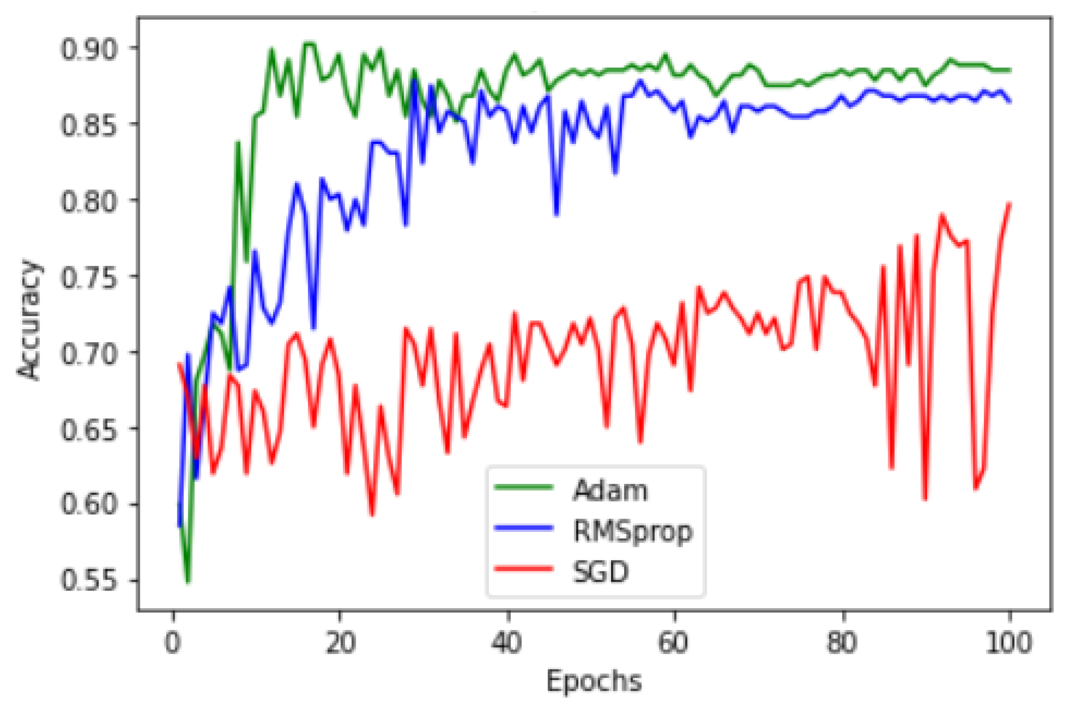
- Sigmoid—this activation function is used to apply such a non-linearity that squeezes the output to a unique value in the range of 0 to 1, corresponding to a unique input value. The equation for the application of this non-linearity can be given below.Finally, we propose the usage of the Adam optimizer (the reason for the usage of the Adam optimizer is depicted in the result and analysis section) and discuss the binary cross entropy loss function next.
- Binary cross-entropy loss—a combination of the sigmoid activation function and cross-entropy loss used for binary classification problems. Hence, the below equation depicts the calculation of the binary cross entropy loss for a sample.where t is the label value, i.e., either 0 (for normal) or 1 (for murmur), depending upon the label of the current input audio signal, and x is the input obtained from the previous layer after application of the sigmoid activation function.
| Algorithm 1: Attention-based Bi-GRU architecture for audio classification |
|
5. Result and Analysis
5.1. Experimentation Setup and Tools
5.2. Simulation Analysis
5.3. Evaluation Metrics
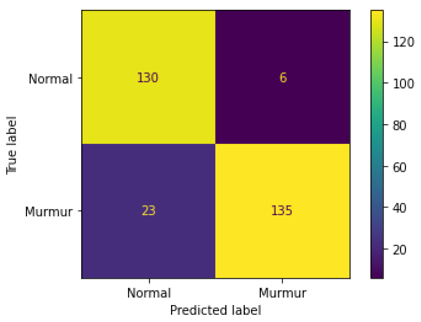
- True Positive ()—labels that are predicted as murmur by the model are truly murmur (bottom right cell of the confusion matrix).
- False Positive ()—labels that are predicted as murmur by the model but are normal (top right cell of the confusion matrix).
- True Negative ()—labels that are predicted as normal by the model are truly normal (top left cell of the confusion matrix).
- False Negative ()—labels that are predicted as normal by the model but are murmur (bottom left cell of the confusion matrix).
- Accuracy—a measure or the ratio of the total number of correct predictions to the total number of predictions performed by a model. A higher accuracy means that a model is more accurate in making predictions. As is evident from Table 2, the validation accuracy of the proposed architecture outperforms others with an acceptable difference in the training accuracy, indicating that the proposed architecture does not overfit as quickly as other models and produces better predictions. Formally, the accuracy is mathematically defined as,
- Precision—the measure of correctly predicted true positive samples out of all predicted true positive samples. Simply, it measures how many predictions are made by the model belonging to a class from that class. Hence, the precision should be as high as possible. From Table 2, it is evident that the proposed architecture outperforms all the other models in precision with a high margin. Formally, precision is defined as,
- Recall—the measure of how many samples belonging to a class that the model predicts as belonging to that class, or simply, it is the ratio of the number of samples of a class that a model identifies out of the total number of samples of that class in the dataset. A high and desirable recall means that a model can extract a high number of samples of a class out of all the samples of that class from the dataset. From Table 2, it is evident that the proposed architecture outperforms all the other models in recall with a high margin. Formally, recall is defined as,
- F1 score—the relation between precision and recall derived from calculating the harmonic mean of precision and recall. The F1 score considers both precision and recall, and a high F1 score is desirable. For the model’s performance, we generally consider the F1 score to be the prime metric of distinction. As is evident from Table 2, the proposed architecture outperforms all the other models in the F1 score with a high margin. Formally, it is defined as,
6. Conclusions
Author Contributions
Funding
Data Availability Statement
Conflicts of Interest
References
- Cardiovascular Diseases (CVDs)—who.int. Available online: https://www.who.int/news-room/fact-sheets/detail/cardiovascular-diseases-(cvds) (accessed on 28 February 2023).
- Vora, J.; Tanwar, S.; Tyagi, S.; Kumar, N.; Rodrigues, J.J. HRIDaaY: Ballistocardiogram-Based Heart Rate Monitoring Using Fog Computing. In Proceedings of the 2019 IEEE Global Communications Conference (GLOBECOM), Waikoloa, HI, USA, 9–13 December 2019; pp. 1–6. [Google Scholar] [CrossRef]
- Fuchs, F.D.; Whelton, P.K. High blood pressure and cardiovascular disease. Hypertension 2020, 75, 285–292. [Google Scholar] [CrossRef] [PubMed]
- Nabel, E.G. Cardiovascular Disease. N. Engl. J. Med. 2003, 349, 60–72. [Google Scholar] [CrossRef] [PubMed]
- Ciumărnean, L.; Milaciu, M.V.; Negrean, V.; Orășan, O.H.; Vesa, S.C.; Sălăgean, O.; Iluţ, S.; Vlaicu, S.I. Cardiovascular Risk Factors and Physical Activity for the Prevention of Cardiovascular Diseases in the Elderly. Int. J. Environ. Res. Public Health 2022, 19, 207. [Google Scholar] [CrossRef] [PubMed]
- Rodgers, J.L.; Jones, J.; Bolleddu, S.I.; Vanthenapalli, S.; Rodgers, L.E.; Shah, K.; Karia, K.; Panguluri, S.K. Cardiovascular Risks Associated with Gender and Aging. J. Cardiovasc. Dev. Dis. 2019, 6, 19. [Google Scholar] [CrossRef] [Green Version]
- Hanna, I.R.; Silverman, M.E. A history of cardiac auscultation and some of its contributors. Am. J. Cardiol. 2002, 90, 259–267. [Google Scholar] [CrossRef]
- Tanwar, S.; Vora, J.; Kaneriya, S.; Tyagi, S.; Kumar, N.; Sharma, V.; You, I. Human Arthritis Analysis in Fog Computing Environment Using Bayesian Network Classifier and Thread Protocol. IEEE Consum. Electron. Mag. 2020, 9, 88–94. [Google Scholar] [CrossRef]
- Vincent, R. I look into the chest: History and evolution of stethoscope. J. Pract. Cardiovasc. Sci. 2022, 8, 168. [Google Scholar]
- Jiang, Z.; Choi, S. A cardiac sound characteristic waveform method for in-home heart disorder monitoring with electric stethoscope. Expert Syst. Appl. 2006, 31, 286–298. [Google Scholar] [CrossRef]
- Kaneriya, S.; Lakhani, D.; Brahmbhatt, H.U.; Tanwar, S.; Tyagi, S.; Kumar, N.; Rodrigues, J.J.P.C. Can Tactile Internet be a Solution for Low Latency Heart Disorientation Measure: An Analysis. In Proceedings of the ICC 2019-2019 IEEE International Conference on Communications (ICC), Shanghai, China, 20–24 May 2019; pp. 1–6. [Google Scholar] [CrossRef]
- Abbas, Q.; Hussain, A.; Baig, A.R. Automatic Detection and Classification of Cardiovascular Disorders Using Phonocardiogram and Convolutional Vision Transformers. Diagnostics 2022, 12, 3109. [Google Scholar] [CrossRef]
- Babu, K.A.; Ramkumar, B.; Manikandan, M.S. Automatic Identification of S1 and S2 Heart Sounds Using Simultaneous PCG and PPG Recordings. IEEE Sens. J. 2018, 18, 9430–9440. [Google Scholar] [CrossRef]
- Kumar, D.; Carvalho, P.; Antunes, M.; Gil, P.; Henriques, J.; Eugenio, L. A New Algorithm for Detection of S1 and S2 Heart Sounds. In Proceedings of the 2006 IEEE International Conference on Acoustics Speech and Signal Processing Proceedings, Toulouse, France, 14–19 May 2006; Volume 2, p. II. [Google Scholar] [CrossRef]
- Zeinali, Y.; Niaki, S.T.A. Heart sound classification using signal processing and machine learning algorithms. Mach. Learn. Appl. 2022, 7, 100206. [Google Scholar] [CrossRef]
- Chen, W.; Sun, Q.; Chen, X.; Xie, G.; Wu, H.; Xu, C. Deep Learning Methods for Heart Sounds Classification: A Systematic Review. Entropy 2021, 23, 667. [Google Scholar] [CrossRef]
- Chauhan, K.; Jani, S.; Thakkar, D.; Dave, R.; Bhatia, J.; Tanwar, S.; Obaidat, M.S. Automated Machine Learning: The New Wave of Machine Learning. In Proceedings of the 2020 2nd International Conference on Innovative Mechanisms for Industry Applications (ICIMIA), Bangalore, India, 5–7 March 2020; pp. 205–212. [Google Scholar] [CrossRef]
- Ren, Z.; Qian, K.; Dong, F.; Dai, Z.; Yamamoto, Y.; Schuller, B.W. Deep Attention-based Representation Learning for Heart Sound Classification. arXiv 2021, arXiv:2101.04979. [Google Scholar]
- Mukherjee, U.; Pancholi, S. A Visual Domain Transfer Learning Approach for Heartbeat Sound Classification. arXiv 2021. [Google Scholar] [CrossRef]
- Kui, H.; Pan, J.; Zong, R.; Yang, H.; Wang, W. Heart sound classification based on log Mel-frequency spectral coefficients features and convolutional neural networks. Biomed. Signal Process. Control 2021, 69, 102893. [Google Scholar] [CrossRef]
- Gupta, R.; Patel, M.M.; Shukla, A.; Tanwar, S. Deep learning-based malicious smart contract detection scheme for internet of things environment. Comput. Electr. Eng. 2022, 97, 107583. [Google Scholar] [CrossRef]
- Jamil, S.; Rahman, M. A Novel Deep-Learning-Based Framework for the Classification of Cardiac Arrhythmia. J. Imaging 2022, 8, 70. [Google Scholar] [CrossRef] [PubMed]
- Xiang, M.; Zang, J.; Wang, J.; Wang, H.; Zhou, C.; Bi, R.; Zhang, Z.; Xue, C. Research of heart sound classification using two-dimensional features. Biomed. Signal Process. Control 2023, 79, 104190. [Google Scholar] [CrossRef]
- Keikhosrokiani, P.; Anathan, A.B.N.A.; Fadilah, S.I.; Manickam, S.; Li, Z. Heartbeat sound classification using a hybrid adaptive neuro-fuzzy inferences system (ANFIS) and artificial bee colony. Digit. Health 2023, 9, 20552076221150741. [Google Scholar] [CrossRef]
- Ballas, A.; Papapanagiotou, V.; Delopoulos, A.; Diou, C. Listen2YourHeart: A Self-Supervised Approach for Detecting Murmur in Heart-Beat Sounds. arXiv 2022. [Google Scholar] [CrossRef]
- Ren, Z.; Qian, K.; Dong, F.; Dai, Z.; Nejdl, W.; Yamamoto, Y.; Schuller, B.W. Deep attention-based neural networks for explainable heart sound classification. Mach. Learn. Appl. 2022, 9, 100322. [Google Scholar] [CrossRef]
- Saraswat, D.; Bhattacharya, P.; Verma, A.; Prasad, V.K.; Tanwar, S.; Sharma, G.; Bokoro, P.N.; Sharma, R. Explainable AI for Healthcare 5.0: Opportunities and Challenges. IEEE Access 2022, 10, 84486–84517. [Google Scholar] [CrossRef]
- Tariq, Z.; Shah, S.K.; Lee, Y. Feature-Based Fusion Using CNN for Lung and Heart Sound Classification. Sensors 2022, 22, 1521. [Google Scholar] [CrossRef] [PubMed]
- Lu, H.; Yip, J.B.; Steigleder, T.; Grießhammer, S.; Sai Jitin Jami, N.; Eskofier, B.; Ostgathe, C.; Koelpin, A. A Lightweight Robust Approach for Automatic Heart Murmurs and Clinical Outcomes Classification from Phonocardiogram Recordings. In Proceedings of the Computing in Cardiology (CinC), Tampere, Finland, 4–7 September 2022; Volume 49. [Google Scholar]
- Milani, M.; Abas, P.E.; De Silva, L.C.; Nanayakkara, N.D. Abnormal heart sound classification using phonocardiography signals. Smart Health 2021, 21, 100194. [Google Scholar] [CrossRef]
- Er, M.B. Heart sounds classification using convolutional neural network with 1D-local binary pattern and 1D-local ternary pattern features. Appl. Acoust. 2021, 180, 108152. [Google Scholar] [CrossRef]
- Xiao, B.; Xu, Y.; Bi, X.; Zhang, J.; Ma, X. Heart sounds classification using a novel 1-D convolutional neural network with extremely low parameter consumption. Neurocomputing 2020, 392, 153–159. [Google Scholar] [CrossRef]
- Tiwari, S.; Sapra, V.; Jain, A. Heartbeat sound classification using Mel-frequency cepstral coefficients and deep convolutional neural network. In Advances in Computational Techniques for Biomedical Image Analysis; Koundal, D., Gupta, S., Eds.; Academic Press: Cambridge, MA, USA, 2020; pp. 115–131. [Google Scholar] [CrossRef]
- Boulares, M.; Alotaibi, R.; AlMansour, A.; Barnawi, A. Cardiovascular Disease Recognition Based on Heartbeat Segmentation and Selection Process. Int. J. Environ. Res. Public Health 2021, 18, 952. [Google Scholar] [CrossRef]
- Schmidt, S.E.; Holst-Hansen, C.; Graff, C.; Toft, E.; Struijk, J.J. Segmentation of heart sound recordings by a duration-dependent hidden Markov model. Physiol. Meas. 2010, 31, 513. [Google Scholar] [CrossRef] [Green Version]
- Chen, T.; Kuan, K.; Celi, L.A.; Clifford, G.D. Intelligent Heartsound Diagnostics on a Cellphone Using a Hands-Free Kit. In Proceedings of the 2010 AAAI Spring Symposium: Artificial Intelligence for Development, Stanford, CA, USA, 22–24 March 2010; Technical Report SS-10-01. AAAI: Palo Alto, CA, USA, 2010. [Google Scholar]
- Moukadem, A.; Dieterlen, A.; Hueber, N.; Brandt, C. A robust heart sounds segmentation module based on S-transform. Biomed. Signal Process. Control 2013, 8, 273–281. [Google Scholar] [CrossRef] [Green Version]
- Safara, F.; Doraisamy, S.; Azman, A.; Jantan, A.; Abdullah Ramaiah, A.R. Multi-level basis selection of wavelet packet decomposition tree for heart sound classification. Comput. Biol. Med. 2013, 43, 1407–1414. [Google Scholar] [CrossRef]
- Ari, S.; Hembram, K.; Saha, G. Detection of cardiac abnormality from PCG signal using LMS based least square SVM classifier. Expert Syst. Appl. 2010, 37, 8019–8026. [Google Scholar] [CrossRef]
- Zhang, W.; Han, J.; Deng, S. Heart sound classification based on scaled spectrogram and tensor decomposition. Expert Syst. Appl. 2017, 84, 220–231. [Google Scholar] [CrossRef]
- Deng, S.W.; Han, J.Q. Towards heart sound classification without segmentation via autocorrelation feature and diffusion maps. Future Gener. Comput. Syst. 2016, 60, 13–21. [Google Scholar] [CrossRef]
- Banerjee, M.; Majhi, S. Multi-class Heart Sounds Classification Using 2D-Convolutional Neural Network. In Proceedings of the 2020 5th International Conference on Computing, Communication and Security (ICCCS), Patna, India, 14–16 October 2020; pp. 1–6. [Google Scholar] [CrossRef]
- Gomes, E.; Bentley, P.; Coimbra, M.; Pereira, E.; Deng, Y. Classifying heart sounds: Approaches to the PASCAL challenge. In Proceedings of the HEALTHINF 2013-Proceedings of the International Conference on Health Informatics, Barcelona, Spain, 11–14 February 2013; pp. 337–340. [Google Scholar]
- Raza, A.; Mehmood, A.; Ullah, S.; Ahmad, M.; Choi, G.S.; On, B.W. Heartbeat Sound Signal Classification Using Deep Learning. Sensors 2019, 19, 4819. [Google Scholar] [CrossRef] [Green Version]
- Zheng, Y.; Guo, X.; Ding, X. A novel hybrid energy fraction and entropy-based approach for systolic heart murmurs identification. Expert Syst. Appl. 2015, 42, 2710–2721. [Google Scholar] [CrossRef]
- Yaseen; Son, G.Y.; Kwon, S. Classification of Heart Sound Signal Using Multiple Features. Appl. Sci. 2018, 8, 2344. [Google Scholar] [CrossRef] [Green Version]
- Xu, Y.; Kong, Q.; Wang, W.; Plumbley, M.D. Large-Scale Weakly Supervised Audio Classification Using Gated Convolutional Neural Network. In Proceedings of the 2018 IEEE International Conference on Acoustics, Speech and Signal Processing (ICASSP), Calgary, AB, Canada, 15–20 April 2018; pp. 121–125. [Google Scholar] [CrossRef] [Green Version]
- Xu, K.; Zhu, B.; Kong, Q.; Mi, H.; Ding, B.; Wang, D.; Wang, H. General audio tagging with ensembling convolutional neural network and statistical features. arXiv 2018, arXiv:1810.12832. [Google Scholar] [CrossRef] [Green Version]
- Chaudhary, S.; Kakkar, R.; Jadav, N.K.; Nair, A.; Gupta, R.; Tanwar, S.; Agrawal, S.; Alshehri, M.D.; Sharma, R.; Sharma, G.; et al. A taxonomy on smart healthcare technologies: Security framework, case study, and future directions. J. Sens. 2022, 2022, 1863838. [Google Scholar] [CrossRef]
- Miller, D.J.; Sargent, C.; Roach, G.D. A Validation of Six Wearable Devices for Estimating Sleep, Heart Rate and Heart Rate Variability in Healthy Adults. Sensors 2022, 22, 6317. [Google Scholar] [CrossRef]
- Karki, S.; Kaariainen, M.; Lekkala, J. Measurement of heart sounds with EMFi transducer. In Proceedings of the 2007 29th Annual International Conference of the IEEE Engineering in Medicine and Biology Society, Lyon, France, 22–26 August 2007; pp. 1683–1686. [Google Scholar] [CrossRef]
- Oliveira, J.; Renna, F.; Costa, P.; Nogueira, M.; Oliveira, A.C.; Elola, A.; Ferreira, C.; Jorge, A.; Rad, A.B.; Reyna, M.; et al. The CirCor DigiScope Phonocardiogram Dataset, Version 1.0.0; PhysioNet: Cambridge, MA, USA, 2022. [Google Scholar]
- Oliveira, J.; Renna, F.; Costa, P.D.; Nogueira, M.; Oliveira, C.; Ferreira, C.; Jorge, A.; Mattos, S.; Hatem, T.; Tavares, T.; et al. The CirCor DigiScope Dataset: From Murmur Detection to Murmur Classification. IEEE J. Biomed. Health Inform. 2022, 26, 2524–2535. [Google Scholar] [CrossRef]
- Shah, H.; Shah, D.; Jadav, N.K.; Gupta, R.; Tanwar, S.; Alfarraj, O.; Tolba, A.; Raboaca, M.S.; Marina, V. Deep Learning-Based Malicious Smart Contract and Intrusion Detection System for IoT Environment. Mathematics 2023, 11, 418. [Google Scholar] [CrossRef]
- Gupta, S.; Jaafar, J.; Wan Ahmad, W.F.; Bansal, A. Feature Extraction Using Mfcc. Signal Image Process. Int. J. 2013, 4, 101–108. [Google Scholar] [CrossRef]
- Bartsch, M.; Wakefield, G. Audio thumbnailing of popular music using chroma-based representations. IEEE Trans. Multimed. 2005, 7, 96–104. [Google Scholar] [CrossRef]
- Hathaliya, J.; Parekh, R.; Patel, N.; Gupta, R.; Tanwar, S.; Alqahtani, F.; Elghatwary, M.; Ivanov, O.; Raboaca, M.S.; Neagu, B.C. Convolutional Neural Network-Based Parkinson Disease Classification Using SPECT Imaging Data. Mathematics 2022, 10, 2566. [Google Scholar] [CrossRef]
- Hathaliya, J.J.; Modi, H.; Gupta, R.; Tanwar, S.; Sharma, P.; Sharma, R. Parkinson and essential tremor classification to identify the patient’s risk based on tremor severity. Comput. Electr. Eng. 2022, 101, 107946. [Google Scholar] [CrossRef]
- McFee, B.; Raffel, C.; Liang, D.; Ellis, D.; Mcvicar, M.; Battenberg, E.; Nieto, O. librosa: Audio and Music Signal Analysis in Python. In Proceedings of the 14th Python in Science Conference, Austin, TX, USA, 6–12 July 2015; pp. 18–24. [Google Scholar] [CrossRef] [Green Version]
- Kingma, D.P.; Ba, J. Adam: A Method for Stochastic Optimization. arXiv 2014, arXiv:1412.6980. [Google Scholar] [CrossRef]
- Papapanagiotou, V.; Diou, C.; Delopoulos, A. Chewing detection from an in-ear microphone using convolutional neural networks. In Proceedings of the 2017 39th Annual International Conference of the IEEE Engineering in Medicine and Biology Society (EMBC), Jeju, Republic of Korea, 11–15 July 2017; pp. 1258–1261. [Google Scholar] [CrossRef]
- Papapanagiotou, V.; Diou, C.; Delopoulos, A. Self-Supervised Feature Learning of 1D Convolutional Neural Networks with Contrastive Loss for Eating Detection Using an In-Ear Microphone. In Proceedings of the 2021 43rd Annual International Conference of the IEEE Engineering in Medicine & Biology Society (EMBC), Virtual, 1–5 November 2021; pp. 7186–7189. [Google Scholar] [CrossRef]


| Model | Train Accuracy | Validation Accuracy | Precision | Recall | F1-Score | AUC | Loss | Accuracy/Loss |
|---|---|---|---|---|---|---|---|---|
| CNN | 87% | 84% | 86% | 85% | 85% | 0.85 | 0.43 | 1.95 |
| LSTM | 87% | 82% | 83% | 82% | 82% | 0.84 | 0.522 | 1.61 |
| BiGRU | 96% | 87% | 87% | 87% | 87% | 0.87 | 0.54 | 1.61 |
| BiLSTM | 95% | 85% | 86% | 85% | 85% | 0.85 | 0.5633 | 1.50 |
| CNN + BiLSTM | 99% | 85% | 85% | 85% | 85% | 0.85 | 0.84 | 1.01 |
| [29] | - | 75.1% | - | - | - | - | - | - |
| [25] | 78.6% | 73.7% | - | - | 65.7% | - | - | - |
| CNN + BiGRU (Proposed model) | 94% | 90% | 90% | 91% | 90% | 0.90 | 0.45 | 2 |
Disclaimer/Publisher’s Note: The statements, opinions and data contained in all publications are solely those of the individual author(s) and contributor(s) and not of MDPI and/or the editor(s). MDPI and/or the editor(s) disclaim responsibility for any injury to people or property resulting from any ideas, methods, instructions or products referred to in the content. |
© 2023 by the authors. Licensee MDPI, Basel, Switzerland. This article is an open access article distributed under the terms and conditions of the Creative Commons Attribution (CC BY) license (https://creativecommons.org/licenses/by/4.0/).
Share and Cite
Yadav, H.; Shah, P.; Gandhi, N.; Vyas, T.; Nair, A.; Desai, S.; Gohil, L.; Tanwar, S.; Sharma, R.; Marina, V.; et al. CNN and Bidirectional GRU-Based Heartbeat Sound Classification Architecture for Elderly People. Mathematics 2023, 11, 1365. https://doi.org/10.3390/math11061365
Yadav H, Shah P, Gandhi N, Vyas T, Nair A, Desai S, Gohil L, Tanwar S, Sharma R, Marina V, et al. CNN and Bidirectional GRU-Based Heartbeat Sound Classification Architecture for Elderly People. Mathematics. 2023; 11(6):1365. https://doi.org/10.3390/math11061365
Chicago/Turabian StyleYadav, Harshwardhan, Param Shah, Neel Gandhi, Tarjni Vyas, Anuja Nair, Shivani Desai, Lata Gohil, Sudeep Tanwar, Ravi Sharma, Verdes Marina, and et al. 2023. "CNN and Bidirectional GRU-Based Heartbeat Sound Classification Architecture for Elderly People" Mathematics 11, no. 6: 1365. https://doi.org/10.3390/math11061365