A Novel Discrete Generator with Modeling Engineering, Agricultural and Medical Count and Zero-Inflated Real Data with Bayesian, and Non-Bayesian Inference

Abstract

This study introduces a unique flexible family of discrete probability distributions for modeling extreme count and zero-inflated count data with different failure rates. Certain significant mathematical properties, such as the cumulant generating function, moment generating function, dispersion index, L-moments, ordinary moments, and central moment are derived. The new failure rate function offers a wide range of flexibility, including “upside down”, “monotonically decreasing”, “bathtub”, “monotonically increasing” and “decreasing-constant failure rate” and “constant”. Moreover, the new probability mass function accommodates many useful shapes including the “right skewed function with no peak”, “symmetric”, “right skewed with one peak” and “left skewed with one peak”. To obtain significant characterization findings, the hazard function and the conditional expectation of certain function of the random variable are both employed. Both Bayesian and non-Bayesian estimate methodologies are considered when estimating, assessing, and comparing inferential efficacy. The Bayesian estimation approach for the squared error loss function is suggested, and it is explained. Markov chain Monte Carlo simulation studies are performed using the Metropolis Hastings algorithm and the Gibbs sampler to compare non-Bayesian vs. Bayesian results. Four real-world applications of count data sets are used to evaluate the Bayesian versus non-Bayesian techniques. Four more real count data applications are used to illustrate the significance and versatility of the new discrete class.

1. Introduction and Genesis

Discrete distributions are important in statistics because they model count data, which arise frequently in many fields, including biology, medicine, social sciences, and engineering. Discrete distributions are also used to model binary data, where the outcome is either zero or one. The importance of discrete distributions can be summarized as follows: Modeling count data: Discrete distributions, such as Poisson and negative binomial, allow us to model count data, which is common in many applications, such as the number of people who visit a website, the number of hospital admissions, or the number of species in a habitat. Modeling binary data: Discrete distributions, such as the binomial and the beta-binomial distributions, allow us to model binary data, which is common in many fields, such as medical trials, social sciences, and marketing. Probabilistic modeling: Discrete distributions provide a probabilistic model for count and binary data, which allows us to make predictions about future events and to assess the uncertainty in these predictions. Estimation and inference: Discrete distributions allow us to estimate parameters of interest, such as the mean and variance, and to make inferences about the population from sample data. In conclusion, discrete distributions play a crucial role in modeling count and binary data and are essential tools for making probabilistic predictions and inferences in many fields of study.

Discretization is the process of converting a continuous variable into a discrete (or categorical) variable by dividing it into intervals. This is an important step in many data analysis and modeling applications for several reasons: Simplification: Discretizing continuous variables can simplify the data and make it easier to understand and interpret. Modeling limitations: Some statistical models, such as linear regression, assume that the variables are continuous, while others, such as logistic regression, assume that the variables are categorical. Discretization can help overcome these limitations. Handling non-linear relationships: Discretization can be used to capture non-linear relationships between variables. For example, if the relationship between two variables is not linear, discretizing one or both of the variables can reveal a relationship that is easier to model. Dimension reduction: Discretization can help reduce the dimensionality of the data, making it easier to visualize and analyze. Handling outliers: Discretization can help handle outliers by transforming them into a smaller number of intervals.

Discretization is an important step in the data pre-processing phase and must be performed carefully to ensure that it does not introduce bias or lose important information. The choice of the number of intervals and the method of discretization can greatly affect the results of the analysis. The discretization of well-known continuous probability distributions has drawn a lot of interest recently. Many researchers have studied a lot of continuous distributions but by discretizing them. This direction was the dominant trend in statistical literature, despite the lack of works in this important field of distribution theory. The importance of discretization of the continuous distributions derives its importance from the presence of a lot of good, engineering, and actuarial data that cannot be dealt with using continuous distributions. This urgent need is the main reason that motivated researchers to move in this direction.

In this context, many discrete type extensions of the continuous models have been presented and studied such as the well-known generalization of the Poisson model (see Consul et al. [1], the discrete type extension of the Weibull distribution (D-W) (see Nakagawa and Osaki [2]), the discrete version of the Rayleigh model (DR) (see Roy [3]), the discrete version of the half-normal model (see Kemp [4] and Kemp [5]), a discrete version of the Pareto distribution (D-Pa) (see Krishna and Pundir Kemp [6]), a novel discrete version of the geometric model (DGc) (see Gómez -Déniz [7] and), a discrete version of the Lindley distribution (D-Li) (see Gómez -Déniz and Calderin-Ojeda [8]), a discrete version of the inverse-Weibull distribution (D-IW) (see Jazi et al. [9]), a discrete version of the exponentiated Weibull distribution (ED-W) (Nekoukhou and Bidram [10]), a discrete version of the generalized exponentiated type II distribution (DGE-II) (see Nekoukhou et al. [11]), a discrete version of the inverse Rayleigh distribution (DIR) (see Hussain and Ahmad [12]), a discrete version of the Lindley type II model (D-Li-II) (Hussain et al. [13]), a discrete version of the Lomax distribution (D-Lx) (Para and Jan [14]), a discrete version of the log-logistic model (DLL) (Para and Jan [15]), a discrete version of the Burr type XII model (D-BXII) (see Para and Jan [15]), a discrete version of the exponentiated Lindley distribution (ED-Li) (see El-Morshedy et al. [16]), a discrete version of the Burr–Hatke model (see El-Morshedy et al. [17]), a discrete version of the generalized Burr–Hatke model (see Yousof et al. [18]), a discrete version of the inverse Burr (DIB) model (see Chesneau et al. [19]), among others.

The distributions above were related to the first trend, as for the second trend, many researchers started to present families of discrete distributions. These families of discrete distributions are not so numerous in the statistical literature that we can exhaustively enumerate them. Therefore, we can limit these families to the following: the discrete Gompertz G family of distributions by Eliwa et al. [20], the discrete Weibull G family by Ibrahim et al. [21], the discrete Rayleigh G by Aboraya et al. [22].

This paper presents and studies a novel discrete family. The continuous generalized Rayleigh family of distributions is the foundation from which the new family is derived. Among the important mathematical elements that are calculated and examined are the ordinary moments, the central moment, the moment generating function, the cumulant generating function, the probability generating function, and the dispersion index (Fano factor). The well-known Weibull model is given particular focus. Some of the traditional (non-Bayesian) estimation techniques that are taken into consideration and researched include the Cramér-von-Mises estimation (CVME), the ordinary least squared estimation (OLSE), the maximum likelihood estimation (MLE), and the weighted least squared estimation (WLSE).

Since there are no conventional ways to obtain the conditional posteriors of the parameters, it is advised to gather samples from the joint posterior of the parameters using a hybrid Markov chain Monte Carlo technique. For the Bayesian estimating approach, the squared error loss function is taken into consideration. Bayesian and non-Bayesian estimates are compared using Markov chain Monte Carlo simulations. The Gibbs sampler and the Metropolis Hastings algorithms are employed. Four genuine data sets are used to illustrate the new family’s adaptability and significance. Compared to the sixteen feuding families, the new family provides a better fit.

Different member distributions could be the subject of future study and discussion. Future research might consider the bivariate and multivariate expansions of this novel family. A RV $X$ is said to have Rayleigh if its cumulative distribution function (CDF) is given by

$$F_{\alpha }\left(𝓍\right)=1-\mathit{exp}\left[-{(\alpha 𝓍)}^2\right]{|}_{\left(𝓍\ge 0 \mathrm{and} \alpha >0\right)}.$$

The CDF of the continuous generalized Rayleigh G (GzRG) family can be expressed as

$$F_{\alpha ,\sigma ,\underset{\_}{\mathit{V}}}\left(𝓍\right)=1-\mathit{exp}\left\{-{\left[\alpha {\mathcal{W}}_{{\sigma }_1,{\sigma }_2,\underset{\_}{\mathit{V}}}\left(𝓍\right)\right]}^2\right\}{|}_{\left(𝓍\in R,\sigma >0\right)}.$$

The function ${\mathcal{W}}_{{\sigma }_1,{\sigma }_2,\underset{\_}{\mathit{V}}}\left(𝓍\right)$ refers to a new odds ratio function, where

$${\mathcal{W}}_{{\sigma }_1,{\sigma }_2,\underset{\_}{\mathit{V}}}(\cdot )=\frac{G_{\underset{\_}{\mathit{V}}}^{{\sigma }_1}(\cdot )}{1-G_{\underset{\_}{\mathit{V}}}^{{\sigma }_2}(\cdot )},$$

and $G_{\underset{\_}{\mathit{V}}}^{}(\cdot )$ refers to the CDF of the baseline model. Therefore, $G_{\underset{\_}{\mathit{V}}}^{{\sigma }_1}(\cdot )$ refers to the exponentiated CDF of the baseline model with power parameter ${\sigma }_1$ and baseline parameter vector $\underset{\_}{\mathit{V}}$, and $G_{\underset{\_}{\mathit{V}}}^{{\sigma }_2}(\cdot )$ refers to the exponentiated CDF of the baseline model with power parameter ${\sigma }_2$ and baseline parameter vector $\underset{\_}{\mathit{V}}$. Let ${\alpha }^2=-\log \left(\mathit{q}\right)$ then, CDF of the discrete generalized Rayleigh G family (DGzR-G) can be expressed as

$$F_{\mathit{q},{\sigma }_1,{\sigma }_2,\underset{\_}{\mathit{V}}}\left(𝓍\right)=1-{\mathit{q}}^{{\mathcal{W}}_{{\sigma }_1,{\sigma }_2,\underset{\_}{\mathit{V}}}^2\left(𝓍+1\right)}{|}_{\left(\mathit{q}\in \left(0,1\right) \mathrm{and} 𝓍\in {\mathit{N}}^{•}=\mathit{N}{{\displaystyle \cup }}^{ }\left\{0\right\}\right)}.$$

(1)

The corresponding survival function (SF) is

$$S_{\mathit{q},\sigma ,\underset{\_}{\mathit{V}}}\left(𝓍\right)={\mathit{q}}^{{\mathcal{W}}_{{\sigma }_1,{\sigma }_2,\underset{\_}{\mathit{V}}}^2\left(𝓍+1\right)}{|}_{\left(\mathit{q}\in \left(0,1\right) \mathrm{and} 𝓍\in {\mathit{N}}^{•}\right)}.$$

(2)

Then, the probability mass function (PMF) of the DGzR-G family corresponding to (2) may be written, thanks to Kemp [5] to obtain the new PMF, as $f_{\mathit{q},{\sigma }_1,{\sigma }_2,\underset{\_}{\mathit{V}}}\left(𝓍\right)=S_{\mathit{q},{\sigma }_1,{\sigma }_2,\underset{\_}{\mathit{V}}}\left(𝓍-1\right)-S_{\mathit{q},{\sigma }_1,{\sigma }_2,\underset{\_}{\mathit{V}}}\left(𝓍\right).$ Therefore, the PMF can be expressed as

$$f_{\mathit{q},{\sigma }_1,{\sigma }_2,\underset{\_}{\mathit{V}}}\left(𝓍\right)={\mathit{q}}^{{\mathcal{W}}_{{\sigma }_1,{\sigma }_2,\underset{\_}{\mathit{V}}}^2\left(𝓍\right)}-{\mathit{q}}^{{\mathcal{W}}_{{\sigma }_1,{\sigma }_2,\underset{\_}{\mathit{V}}}^2\left(𝓍+1\right)}{|}_{\left(\mathit{q}\in \left(0,1\right) \mathrm{and} 𝓍\in {\mathit{N}}^{•}\right)},$$

(3)

where ${\mathcal{W}}_{{\sigma }_1,{\sigma }_2,\underset{\_}{\mathit{V}}}^{}(.)$ refers to the generated odd ratio function of any discrete non-negative random variable (DNNRV). The DGzR-G family’s hazard rate function (HRF) is ${\mathit{𝒽}}_{\mathit{q},{\sigma }_1,{\sigma }_2,\underset{\_}{\mathit{V}}}\left(𝓍\right)=f_{\mathit{q},{\sigma }_1,{\sigma }_2,\underset{\_}{\mathit{V}}}\left(𝓍\right)/S_{\mathit{q},{\sigma }_1,{\sigma }_2,\underset{\_}{\mathit{V}}}\left(𝓍-1\right)$, or

$${\mathit{𝒽}}_F\left(𝓍\right)={\mathit{𝒽}}_{\mathit{q},{\sigma }_1,{\sigma }_2,\underset{\_}{\mathit{V}}}\left(𝓍\right)=1-{\mathit{q}}^{{\mathcal{W}}_{{\sigma }_1,{\sigma }_2,\underset{\_}{\mathit{V}}}^2\left(𝓍+1\right)-{\mathcal{W}}_{{\sigma }_1,{\sigma }_2,\underset{\_}{\mathit{V}}}^2\left(𝓍\right)}.$$

(4)

Even though there are a lot of discrete distributions in the statistical literature, discrete G families are still rare (where G = $G_{\underset{\_}{\mathit{V}}}^{}(\cdot )$ refers to CDF of any baseline model); this is because there are not a lot of discrete G families in the literature. The reasons for our introduction the DGzR-G family are as follows:

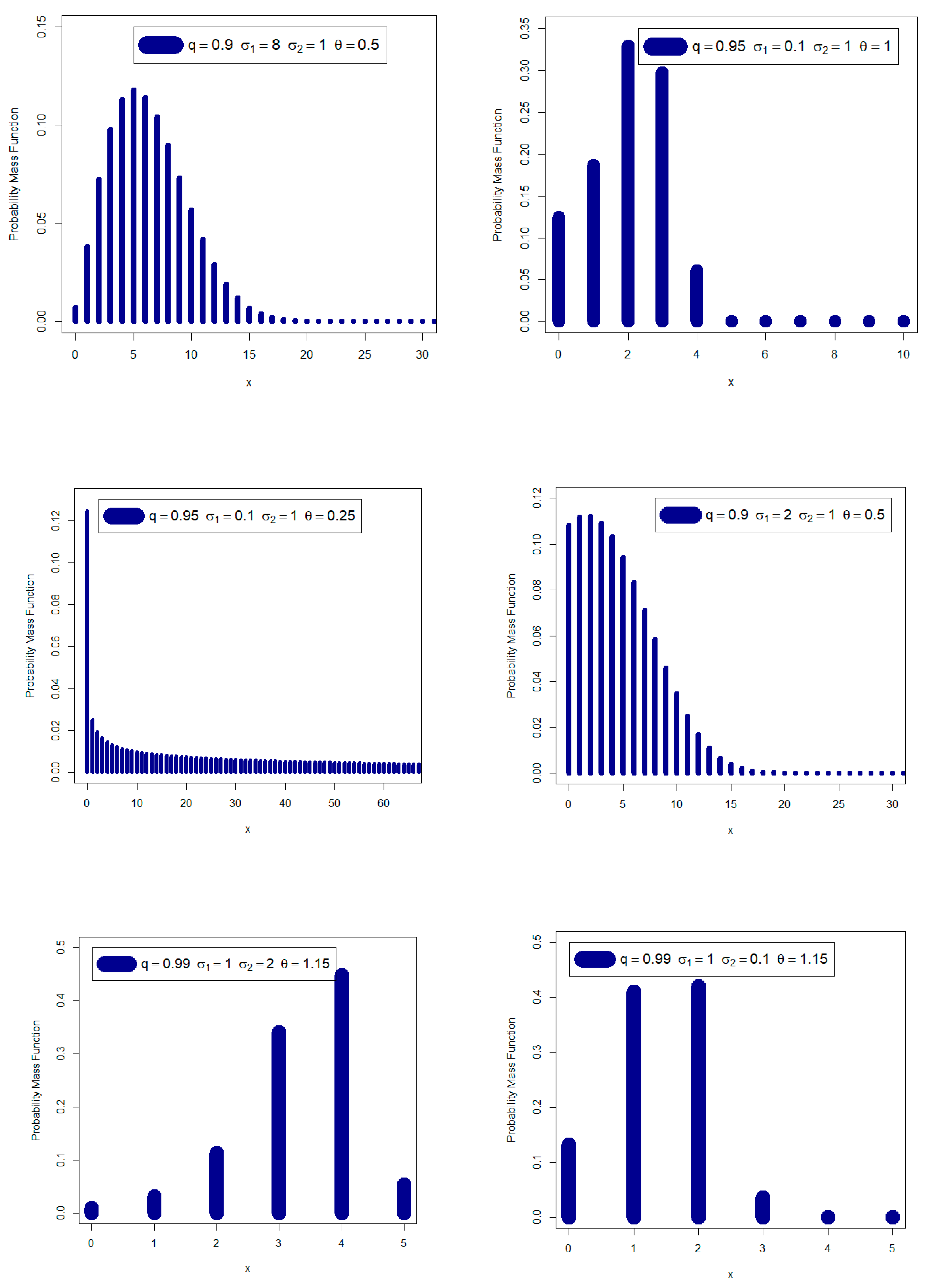
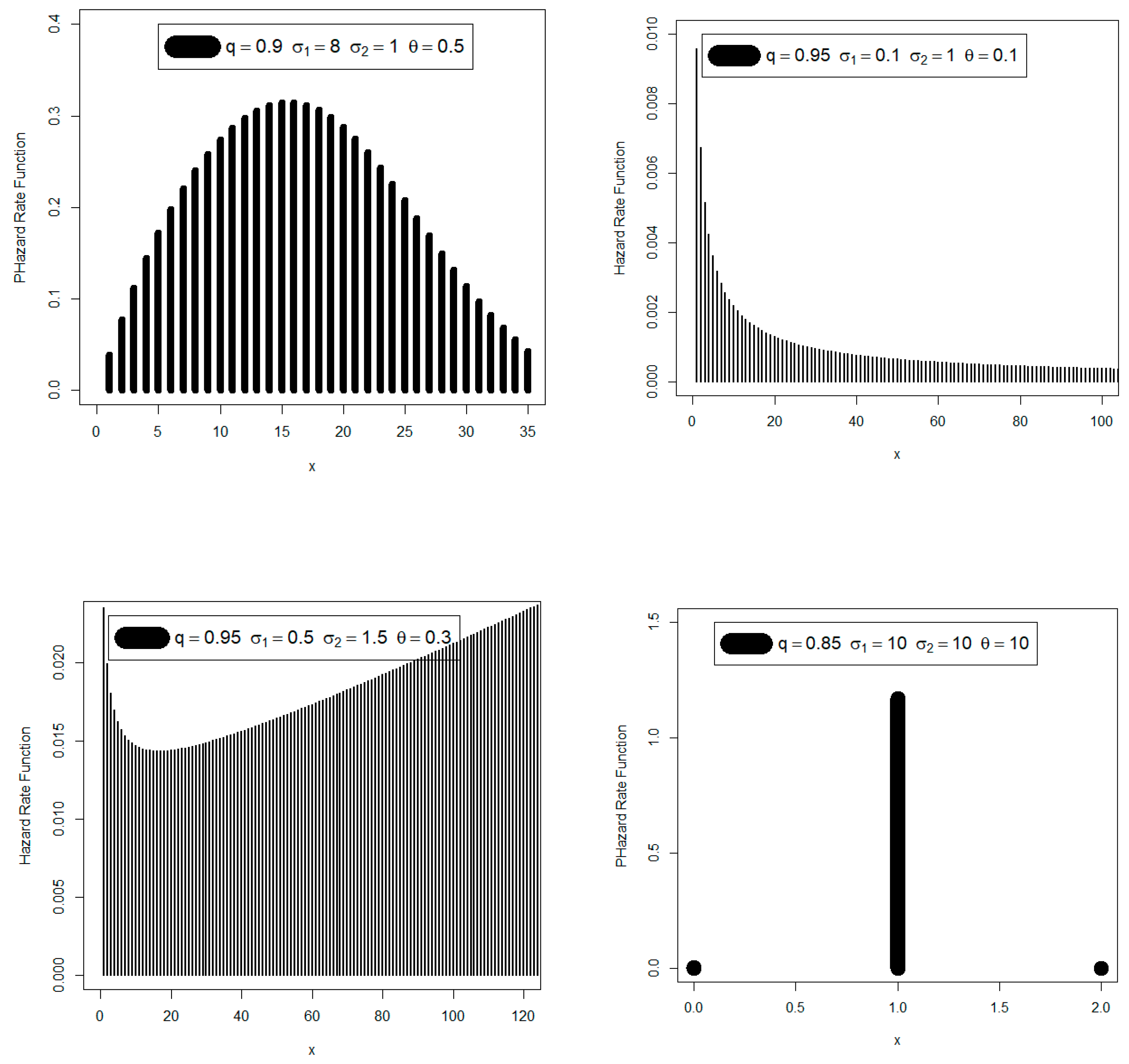
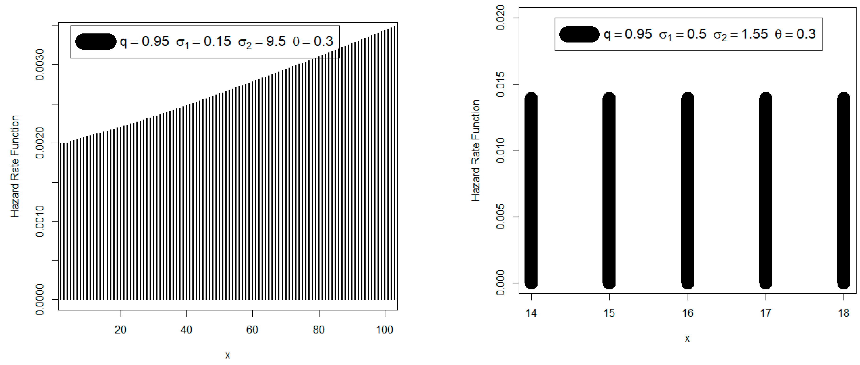
• Creating new probability mass functions that can be, among other helpful forms such as “right skewed probability mass function with no peak”, “symmetric probability mass function”, “right probability mass function skewed with one peak” and “left skewed with one peak”. We may utilize the innovative DGzR-G family’s variable probability mass function to examine a range of count environmental data. Introducing some new models that have various hazard rate shapes including “upside down failure rate”, “monotonically decreasing failure rate”, “bathtub failure rate”, “monotonically increasing failure rate” and “decreasing-constant failure rate” and “constant failure rate with one value”. The diversity in the failure rate function gives the probability distribution a great advantage and a high superiority in the statistical and mathematical modeling processes. This feature is enjoyed by the new family, which makes it qualified to model many count data.
• The new distribution’s flexibility is really influenced by a number of factors, including the size of the skew coefficient, kurtosis coefficient, failure rate function, and variations of the PMF and failure rate function. In this case, it is equally important to apply and effectively use the probability distribution in mathematical analysis. We found that the novel probability mass function was highly adaptable in these and other areas when we examined more closely. This inspired us to thoroughly investigate this probability distribution.
• To represent real data that is “over-dispersed,” “equal-dispersed,” and “under-dispersed,” some new discrete models are presented. No matter how symmetric or asymmetric the data are or whether they contain outliers, it is obvious that the DGzR-G family has demonstrated to be more economical at modelling many types of data.
• The cornerstone of a statistical model known as a zero-inflated model in statistics is a zero-inflated probability distribution, or distribution that allows multiple zero-valued observations. For instance, the number of insurance claims within a community for a specific type of risk would be zero-inflated if people who are unable to file a claim because they have not acquired insurance against the risk. In this work, we are inspired to utilize the novel family instead of the zero-inflated Poisson regression model, which is frequently used to model and forecast zero-inflated count data.
• Compare the estimating techniques for both simulated and real-count/zero-inflated data for suggesting and recommending the most appropriate method in each situation.
• Since the novel family produced satisfactory results in the statistical modelling of the data, it is recommended for use in analyzing the bathtub hazard rate count data (under the Weibull baseline model). The data displaying a monotonically increasing failure rate count may also be adequately explained by the same fundamental concept.
• The new family can be considered as a suitable statistical alternative for handling the zero-inflated and count medical data with a decreasing failure rate and certain some outlier observations.
• The new class was a suitable choice for modeling zero-inflated agricultural data that has a decreasing–increasing–decreasing failure rate and contains some outliers.
• In fact, we experimentally show that the proposed G family of distributions matches more closely four real data sets than the other sixteen extended competitive distributions with three and four parameters.
• For the estimate and statistical inference side, other traditional (non-Bayesian) estimating techniques are taken into account. This would include weighted-least squares estimation, ordinary least squares estimation, and maximum likelihood estimation. Additionally considered is the Bayesian estimate under the squared error loss function. The common Markov chain Monte Carlo simulations are used to compare the Bayesian and traditional methods. Using four actual data sets, the applicability of the DGzR-G family is shown and explained. Due to the consistency of the Akaike information criteria, Chi-square, Kolmogorov–Smirnov, and its associated P-value(PV), the DGzR-G family under the Weibull model environment provided a better fit than many competing models.

The rest of this paper is structured as follows. A few mathematical traits of the DGzR-G family are inferred and studied in Section 2. Several characterization findings are reported in Section 3 of the paper. Techniques for estimate and inference are presented in Section 4. Bayesian and non-Bayesian estimate methods are contrasted using Markov chain Monte Carlo simulations in Section 5. Four data examples are presented in Section 6 to compare Bayesian and non-Bayesian estimation methods. In Section 7, two count applications for contrasting the competing discrete models are considered. In Section 8, two Zero-inflated applications for contrasting the competing discrete models are considered. Section 9 gives some concluding remarks.

2. Properties

2.1. Raw Moments

In order to deal with the mathematical and statistical characteristics of the new family, we will present some sub-sections for each property separately.

Theorem 1. 

Let$X$be DNNRV, where$X\sim$DGzR-G ($\mathit{q},{\sigma }_1,{\sigma }_2,\underset{\_}{\mathit{V}}$) family, then the${𝓈}^{\mathrm{th}}$moment of$X$can be expressed as

$$E\left(X^{𝓈}\right)={\mu }_{𝓈,X}^{\prime }={\displaystyle \sum }_{𝓍=1}^{\infty }\left[{𝓍}^{𝓈}-{\left(𝓍-1\right)}^{𝓈}\right]{\mathit{q}}^{{\mathcal{W}}_{{\sigma }_1,{\sigma }_2,\underset{\_}{\mathit{V}}}^2\left(𝓍\right)}{|}_{\left(𝓍\in {\mathit{N}}^{•},\mathit{q}\in \left(0,1\right) \mathrm{and} 𝓈=1,2,3,\dots \right)}.$$

(5)

Proof. 

Since

$$E\left(X^{𝓈}\right)={\mu }_{𝓈,X}^{\prime }={\displaystyle \sum }_{𝓍=0}^{\infty }{𝓍}^{𝓈}{S}_{\mathit{q},{\sigma }_1,{\sigma }_2,\underset{\_}{\mathit{V}}}\left(𝓍\right).$$

Then,

$$E\left(X^{𝓈}\right)={\mu }_{𝓈,X}^{\prime }={\displaystyle \sum }_{𝓍=0}^{\infty }{𝓍}^{𝓈}\left[{\mathit{q}}^{{\mathcal{W}}_{{\sigma }_1,{\sigma }_2,\underset{\_}{\mathit{V}}}^2\left(𝓍\right)}-{\mathit{q}}^{{\mathcal{W}}_{{\sigma }_1,{\sigma }_2,\underset{\_}{\mathit{V}}}^2\left(𝓍+1\right)}\right]={\displaystyle \sum }_{𝓍=1}^{\infty }\left[{𝓍}^{𝓈}-{\left(𝓍-1\right)}^{𝓈}\right]S_{\mathit{q},{\sigma }_1,{\sigma }_2,\underset{\_}{\mathit{V}}}\left(𝓍-1\right).$$

Then,

$$E\left(X^{𝓈}\right)={\mu }_{𝓈,X}^{\prime }={\displaystyle \sum }_{𝓍=1}^{\infty }\left[{𝓍}^{𝓈}-{\left(𝓍-1\right)}^{𝓈}\right]{\mathit{q}}^{{\mathcal{W}}_{{\sigma }_1,{\sigma }_2,\underset{\_}{\mathit{V}}}^2\left(𝓍\right)}{|}_{\left(𝓍\in {\mathit{N}}^{•},\mathit{q}\in \left(0,1\right) \mathrm{and} 𝓈=1,2,3,\dots \right)},$$

end Proof. □

Then, using (5), the mean ($E\left(X\right)={\mu }_{1,X}^{\prime }$), and $E\left(X^2\right)={\mu }_{2,X}^{\prime }$ can be, respectively, written as

$$E\left(X\right)={\mu }_{1,X}^{\prime }={\displaystyle \sum }_{𝓍=1}^{\infty }{\mathit{q}}^{{\mathcal{W}}_{{\sigma }_1,{\sigma }_2,\underset{\_}{\mathit{V}}}^2\left(𝓍\right)}{|}_{\left(𝓍\in {\mathit{N}}^{•},\mathit{q}\in \left(0,1\right) \mathrm{and} 𝓈=1\right)},$$

and

$$E\left(X^2\right)={\mu }_{2,X}^{\prime }={\displaystyle \sum }_{𝓍=1}^{\infty }\left(2𝓍-1\right){\mathit{q}}^{{\mathcal{W}}_{{\sigma }_1,{\sigma }_2,\underset{\_}{\mathit{V}}}^2\left(𝓍\right)}{|}_{\left(𝓍\in {\mathit{N}}^{•},\mathit{q}\in \left(0,1\right) \mathrm{and} 𝓈=2\right)},$$

where the prime in ${\mu }_{𝓈,X}^{\prime }$ for referring to the ${𝓈}^{\mathrm{th}}$ raw moment of $X$. On the other hand, we have the same notations without prime (${\mu }_{𝓈,X}$) for referring to the ${𝓈}^{\mathrm{th}}$ central moments.

2.2. Central Moments

The ${𝓈}^{\mathrm{th}}$ central moment of the random variable $X$, say ${\mu }_{𝓈,X}$, can be derived as

$$E{(X-{\mu }_{1,X}^{\prime })}^{𝓈}={\mu }_{𝓈,X}={\displaystyle \sum }_{\mathcal{O}=0}^{𝓈}{\left(-{\mu }_1^{\prime }\right)}^{\mathit{𝒽}}\left(\begin{array}{c}𝓈\\ \mathcal{O}\end{array}\right){\mu }_{𝓈-\mathcal{O}}^{\prime }{|}_{\left({|}_{\left(𝓍\in {\mathit{N}}^{•},\mathit{q}\in \left(0,1\right) \mathrm{and} 𝓈=1,2,3,\dots \right)}\right)}.$$

So, the variance ($\mathit{V}\left(X\right)$) from

$$E{\left(X-{\mu }_{1,X}^{\prime }\right)}^2=\hspace{0.17em}{\mu }_{2,X}={\displaystyle \sum }_{\mathcal{O}=0}^{𝓈}{\left(-{\mu }_1^{\prime }\right)}^{\mathit{𝒽}}\left(\begin{array}{c}2\\ \mathcal{O}\end{array}\right){\mu }_{2-\mathcal{O}}^{\prime }{|}_{\left({|}_{\left(𝓍\in {\mathit{N}}^{•},\mathit{q}\in \left(0,1\right) \mathrm{and} 𝓈=2\right)}\right)},$$

Moreover, the $\mathit{V}\left(X\right)$ can be derived using the ordinary moments as follows:

$${\mu }_{2,X}=\mathit{V}\left(X\right)={\mu }_{2,X}^{\prime }-{\left({\mu }_{1,X}^{\prime }\right)}^2={\displaystyle \sum }_{𝓍=1}^{\infty }\left(2𝓍-1\right){\mathit{q}}^{{\mathcal{W}}_{{\sigma }_1,{\sigma }_2,\underset{\_}{\mathit{V}}}^2\left(𝓍\right)}-{\left({\displaystyle \sum }_{𝓍=1}^{\infty }{\mathit{q}}^{{\mathcal{W}}_{{\sigma }_1,{\sigma }_2,\underset{\_}{\mathit{V}}}^2\left(𝓍\right)}\right)}^2{|}_{\left(𝓍\in {\mathit{N}}^{•},\mathit{q}\in \left(0,1\right) \mathrm{and} 𝓈=2\right)}.$$

The Fano factor (FF) or the variance to mean ratio (VMR) of the DGzR-G family can be derived as

$$\mathrm{FF}\left(X\right)=\frac{{{\displaystyle \sum }}_{𝓍=1}^{\infty }\left(2𝓍-1\right){\mathit{q}}^{{\mathcal{W}}_{{\sigma }_1,{\sigma }_2,\underset{\_}{\mathit{V}}}^2\left(𝓍\right)}}{{{\displaystyle \sum }}_{𝓍=1}^{\infty }{\mathit{q}}^{{\mathcal{W}}_{{\sigma }_1,{\sigma }_2,\underset{\_}{\mathit{V}}}^2\left(𝓍\right)} }-{\displaystyle \sum }_{𝓍=1}^{\infty }{\mathit{q}}^{{\mathcal{W}}_{{\sigma }_1,{\sigma }_2,\underset{\_}{\mathit{V}}}^2\left(𝓍\right)}{|}_{\left(𝓍\in {\mathit{N}}^{•} \mathrm{and} \mathit{q}\in \left(0,1\right)\right)}.$$

The index of dispersion, also known as the FF, coefficient of dispersion, relative variance, or variance-to-mean ratio (VMR), is a normalized measure of the dispersion of a probability distribution that is used in probability theory and statistics to determine whether a set of observed occurrences is clustered or dispersed in comparison to a common statistical model. When describing the distribution of events or objects in time or space, the VMR is utilized and provides us some useful information. The FF is approximately 1 if the distribution is random, that is, if it can be represented by the Poisson process or one of its multidimensional counterparts. Greater results (FF > 1) indicate the presence of geographical or temporal clusters or “clumps”. Smaller values of the FF (1 > FF) represent a distribution that is more equal or uniform than random, or mutual “avoidance” of occurrences or objects in time or space. The essential characteristic of the Poisson distribution, that the variance and mean are equal, gives rise to these characteristics of FF. The Variance/Mean Ratio test makes use of the FF.

2.3. The Moment Generating Function (MGF) and Cumulant Generating Function (CGF)

Theorem 2. 

Let$X$be DNNRV, where$X\sim$DGzR-G ($\mathit{q},{\sigma }_1,{\sigma }_2,\underset{\_}{\mathit{V}}$) family, then the MGF of$X$can be obtained as

$$M_X\left(t\right)=1+{\displaystyle \sum }_{𝓍=1}^{\infty }\left\{\mathit{exp}\left(tX\right)-\mathit{exp}\left[t\left(X-1\right)\right]\right\}{\mathit{q}}^{{\mathcal{W}}_{{\sigma }_1,{\sigma }_2,\underset{\_}{\mathit{V}}}^2\left(𝓍\right)}{|}_{\left(𝓍\in {\mathit{N}}^{•},\mathit{q}\in \left(0,1\right) \mathrm{and} 𝓈=1,2,3,\dots \right)}.$$

(6)

Proof. 

The MGF of our DNNRV $X$ can be derived from

$$M_X\left(t\right)={\displaystyle \sum }_{𝓍=0}^{\infty }\mathit{exp}\left(tX\right)S_{\mathit{q},{\sigma }_1,{\sigma }_2,\underset{\_}{\mathit{V}}}\left(𝓍\right).$$

Using (3) we have

$$M_X\left(t\right)={\displaystyle \sum }_{𝓍=0}^{\infty }\mathit{exp}\left(tX\right)\left[{\mathit{q}}^{{\mathcal{W}}_{{\sigma }_1,{\sigma }_2,\underset{\_}{\mathit{V}}}^2\left(𝓍\right)}-{\mathit{q}}^{{\mathcal{W}}_{{\sigma }_1,{\sigma }_2,\underset{\_}{\mathit{V}}}^2\left(𝓍+1\right)}\right],$$

then

$$\begin{gathered} M_X\left(t\right)=1+{\displaystyle \sum }_{𝓍=1}^{\infty }\left\{\mathit{exp}\left(tX\right) \\ \hspace{1em}\hspace{1em}\hspace{1em}\hspace{1em}\hspace{1em}\hspace{1em}\hspace{1em}\hspace{1em}\hspace{1em}\hspace{1em}\hspace{1em}\hspace{1em}\hspace{1em}\hspace{1em}\hspace{1em}\hspace{1em}\hspace{1em}\hspace{1em}\hspace{1em}\hspace{1em}\hspace{1em}\hspace{1em}-\mathit{exp}\left[t\left(X-1\right)\right]\right\}{\mathit{q}}^{{\mathcal{W}}_{{\sigma }_1,{\sigma }_2,\underset{\_}{\mathit{V}}}^2\left(𝓍\right)}{|}_{\left(𝓍\in {\mathit{N}}^{•},\mathit{q}\in \left(0,1\right) \mathrm{and} 𝓈=1,2,3,\dots \right)}, \end{gathered}$$

end Proof. □

The first $𝓈$ derivatives of (6), with respect to $t$|$t=0$, yield the first 𝓈 raw moments, i.e.,

$${\mu }_{𝓈,X}^{\prime }=E\left(X^{𝓈}\right)=\frac{{\mathcal{O}}^{𝓈}}{\mathcal{O}{t}^{𝓈}}{M}_X\left(t\right){|}_{\left(t=0 \mathrm{and} 𝓈=1,2,3,\dots \right)},$$

where

$${\mu }_{1,X}^{\prime }=E\left(X\right)=\frac{\mathcal{O}}{\mathcal{O}t}{M}_X\left(t\right){|}_{t=0}={\displaystyle \sum }_{𝓍=1}^{\infty }{\mathit{q}}^{{\mathcal{W}}_{{\sigma }_1,{\sigma }_2,\underset{\_}{\mathit{V}}}^2\left(𝓍\right)}{|}_{\left(𝓍\in {\mathit{N}}^{•},\mathit{q}\in \left(0,1\right) \mathrm{and} 𝓈=1\right)},$$

$$\begin{gathered} {\mu }_{2,X}^{\prime }=E\left(X^2\right)=\frac{{\mathcal{O}}^2}{\mathcal{O}{t}^2}{M}_X\left(t\right){|}_{\left(t=0\right)} \\ \hspace{1em}\hspace{1em}\hspace{1em}\hspace{1em}\hspace{1em}\hspace{1em}\hspace{1em}\hspace{1em}\hspace{1em}\hspace{1em}\hspace{1em}\hspace{1em}\hspace{1em}\hspace{1em}\hspace{1em}\hspace{1em}\hspace{1em}\hspace{1em}={\displaystyle \sum }_{𝓍=1}^{\infty }\left(2𝓍-1\right){\mathit{q}}^{{\mathcal{W}}_{{\sigma }_1,{\sigma }_2,\underset{\_}{\mathit{V}}}^2\left(𝓍\right)}{|}_{\left(𝓍\in {\mathit{N}}^{•},\mathit{q}\in \left(0,1\right) \mathrm{and} 𝓈=2\right)}, \end{gathered}$$

$${\mu }_{3,X}^{\prime }=E\left(X^3\right)=\frac{{\mathcal{O}}^3}{\mathcal{O}{t}^3}{M}_X\left(t\right){|}_{\left(t=0\right)}={\displaystyle \sum }_{𝓍=1}^{\infty }\left[3𝓍\left(𝓍-1\right)+1\right]{\mathit{q}}^{{\mathcal{W}}_{{\sigma }_1,{\sigma }_2,\underset{\_}{\mathit{V}}}^2\left(𝓍\right)}{|}_{\left(𝓍\in {\mathit{N}}^{•},\mathit{q}\in \left(0,1\right) \mathrm{and} 𝓈=3\right)},$$

and

$${\mu }_{4,X}^{\prime }=E\left(X^4\right)=\frac{{\mathcal{O}}^4}{\mathcal{O}{t}^4}{M}_X\left(t\right){|}_{\left(t=0\right)}={\displaystyle \sum }_{𝓍=1}^{\infty }\left[{𝓍}^4-{\left(𝓍-1\right)}^4\right]{\mathit{q}}^{{\mathcal{W}}_{{\sigma }_1,{\sigma }_2,\underset{\_}{\mathit{V}}}^2\left(𝓍\right)}{|}_{\left(𝓍\in {\mathit{N}}^{•},\mathit{q}\in \left(0,1\right) \mathrm{and} 𝓈=4\right)}.$$

Clearly, by taking the logarithm of $M_X\left(t\right),$ we obtain the CGF. Thus, the ${𝓈}^{\mathrm{th}}$ cumulant, say $U_{𝓈,X}$, can be obtained from $U_{𝓈,X}=\frac{{\mathcal{O}}^{𝓈}}{\mathcal{O}{t}^{𝓈}}\log \left[M_X\left(t\right)\right]{|}_{\left(t=0, \mathrm{and} 𝓈=1,2,3,\dots \right)}.$ Regarding the 1st cumulant: the 1st cumulant ($U_{1,X}$) is the mean (${\mu }_{1,X}^{\prime }$). Regarding the $2\mathrm{nd}$ cumulant: the $2\mathrm{nd}$ cumulant ($U_{2,X}$) is the same as the variance ($\mathit{V}ar\left(X\right)$). Regarding the $3\mathrm{rd}$ cumulant: the $3\mathrm{rd}$ cumulant ($U_{3,X}$) is the same as the $3\mathrm{rd}$ central moment, then, $U_{3,X}={\mu }_{3,X}$, that being $U_{1,X}={\mu }_{1,X}^{\prime }=E\left(X\right), U_{2,X}={\mu }_{2,X}={\mu }_{2,X}^{\prime }-{\mu }_{1,X}^{\prime 2}$ and $U_{3,X}={\mu }_{3,X}={\mu }_{3,X}^{\prime }-3{\mu }_{2,X}^{\prime }{\mu }_{1,X}^{\prime }+2{\mu }_{1,X}^{\prime 3}.$ However, the 4th cumulant, 3th and higher order cumulants are not equal to their corresponding central moments. In certain circumstances, theoretical solutions to issues that use cumulants instead of moments are more straightforward, especially when there are two or more statistically independent RVs; the ${𝓈}^{\mathrm{th}}$ order cumulant of their sum is equal to the sum of their ${𝓈}^{\mathrm{th}}$ order cumulants. Moreover, the cumulants can also be obtained from $U_{𝓈,X}{|}_{𝓈\ge 1}={\mu }_{𝓈,X}^{\prime }-{\displaystyle \sum }_{\mathit{𝒽}=0}^{𝓈-1}\left(\begin{array}{c}𝓈-1\\ \mathit{𝒽}-1\end{array}\right){\mu }_{𝓈-\mathit{𝒽},X}^{\prime }{U}_{\mathit{𝒽},X}.$ It is possible to write the probability generating function as

$$P_X\left(𝓈\right)=1+{\displaystyle \sum }_{𝓍=1}^{\infty }\left(1-\frac{1}{𝓈}\right){𝓈}^{𝓍}{\mathit{q}}^{{\mathcal{W}}_{\sigma ,\underset{\_}{\mathit{V}}}^2\left(𝓍\right)}{|}_{\left(𝓍\in {\mathit{N}}^{•},\mathit{q}\in \left(0,1\right) \mathrm{and} 𝓈=1,2,3,\dots \right)}.$$

Numerous fields, including computer science, information theory, quantum information, survival analysis, and econometrics, have used the probability generating function. In a separate article, it is feasible to construct and conduct research on the measure of variation of the uncertainty of the random variable $X$.

2.4. The L-moments

L-moments can be derived and used in a similar way to how ordinary moments are. To estimate the L-moments, one alternative is to combine the order statistics linearly. Every time the distribution’s mean is present, the L-moments exist. There are an endless number of weighted linear combinations of the means of the relevant DGzR-G order statistics that may be used to create explicit formulae for the L-moments. As a linear function of the L-moments, the expected order statistics may be stated as follows:

$$L{M}_{𝓈,X}=\frac{1}{𝓈}{\displaystyle \sum }_{\mathcal{Q}=0}^{𝓈-1}E\left(X_{\left(𝓈-\mathcal{Q}:\mathcal{Q}\right)}\left(\mathit{q},{\sigma }_1,{\sigma }_2,\underset{\_}{\mathit{V}}\right)\right)\mathcal{W}\left(𝓈-1,\mathcal{Q}\right){|}_{\hspace{0.17em}𝓈\ge 1},$$

where $\mathcal{W}\left(𝓈-1,\mathcal{Q}\right)={\left(-1\right)}^{\mathcal{Q}}\left(\begin{array}{c}𝓈-1\\ \mathcal{Q}\end{array}\right)$. The first four L-moments can be expressed as:

$$L{M}_{1,X}=E\left(X_{\left(1:1\right)}\left(\mathit{q},{\sigma }_1,{\sigma }_2,\underset{\_}{\mathit{V}}\right)\right),$$

$$L{M}_{2,X}=\frac{1}{2}E\left(X_{\left(2:2\right)}\left(\mathit{q},{\sigma }_1,{\sigma }_2,\underset{\_}{\mathit{V}}\right)-X_{\left(1:2\right)}\left(\mathit{q},{\sigma }_1,{\sigma }_2,\underset{\_}{\mathit{V}}\right)\right),$$

$$L{M}_{3,X}=M_3\left(X\right)=\frac{1}{3}E\left(X_{\left(3:3\right)}\left(\mathit{q},{\sigma }_1,{\sigma }_2,\underset{\_}{\mathit{V}}\right)+X_{\left(1:3\right)}\left(\mathit{q},{\sigma }_1,{\sigma }_2,\underset{\_}{\mathit{V}}\right)-2X_{\left(2:3\right)}\left(\mathit{q},{\sigma }_1,{\sigma }_2,\underset{\_}{\mathit{V}}\right)\right),$$

and

$$L{M}_{4,X}=M_4\left(X\right)=\frac{1}{4}E\left(X_{\left(4:4\right)}\left(\mathit{q},{\sigma }_1,{\sigma }_2,\underset{\_}{\mathit{V}}\right)-3X_{\left(3:4\right)}\left(\mathit{q},{\sigma }_1,{\sigma }_2,\underset{\_}{\mathit{V}}\right)-X_{\left(1:4\right)}\left(\mathit{q},{\sigma }_1,{\sigma }_2,\underset{\_}{\mathit{V}}\right)+3X_{\left(2:4\right)}\left(\mathit{q},{\sigma }_1,{\sigma }_2,\underset{\_}{\mathit{V}}\right)\right).$$

2.5. A Special Case

For the standard Weibull baseline model, it is seen that ${\mathcal{W}}_{{\sigma }_1,{\sigma }_2, \theta }\left(𝓍\right)=\frac{{\left[1-\mathit{exp}\left(-{𝓍}^{\theta }\right)\right]}^{{\sigma }_1}}{1-{\left[1-\mathit{exp}\left(-{𝓍}^{\theta }\right)\right]}^{{\sigma }_2}}{|}_{𝓍\in {\mathit{N}}^{•},\mathit{q}\in \left(0,1\right),\theta >0}$. Then based on (3), the PMF of the discrete generalized Rayleigh Weibull (DGzR-W) model can be expressed as $f_{\mathit{q},{\sigma }_1,{\sigma }_2,\theta }\left(𝓍\right)={\mathit{q}}^{{\mathcal{W}}_{{\sigma }_1,{\sigma }_2, \theta }^2\left(𝓍\right)}-{\mathit{q}}^{{\mathcal{W}}_{{\sigma }_1,{\sigma }_2, \theta }^2\left(𝓍+1\right)} {|}_{\left(𝓍\in {\mathit{N}}^{•},\mathit{q}\in \left(0,1\right) \mathrm{and} {\sigma }_1,{\sigma }_2,\theta >0\right)}, {\mathcal{W}}_{{\sigma }_1,{\sigma }_2, \theta }^2\left(𝓍\right)={\left\{\frac{{\left[1-\mathit{exp}\left(-{𝓍}^{\theta }\right)\right]}^{{\sigma }_1}}{1-{\left[1-\mathit{exp}\left(-{𝓍}^{\theta }\right)\right]}^{{\sigma }_2}}\right\}}^{-2}$ and ${\mathcal{W}}_{{\sigma }_1,{\sigma }_2, \theta }^2\left(𝓍+1\right)={\left\{\frac{{\left\{1-\mathit{exp}\left[-{\left(𝓍+1\right)}^{\theta }\right]\right\}}^{{\sigma }_1}}{1-{\left\{1-\mathit{exp}\left[-{\left(𝓍+1\right)}^{\theta }\right]\right\}}^{{\sigma }_2}}\right\}}^2$. Clearly, when $\theta =1$, the DGzR-W model reduced to the DGzR-exponential model. The PMF of the DGzR-W model is plotted in Figure 1 for some parameter values. Figure 2 displays some plots of the DGzR-W model’s HRF for selected parameter values. Based on Figure 1, we note that the PMF of the DGzR-W can be “symmetric probability mass function”, “right skewed probability mass function with no peak”, “right probability mass function skewed with one peak” and “left skewed with one peak”. Based on Figure 2, we note that the HRF of the DGzR-W can be “upside down hazard rate function”, “monotonically decreasing hazard rate function“, “decreasing-constant-increasing (U-hazard rate function)”, “monotonically increasing hazard rate function“ and “decreasing-constant” and “constant with one value”.

The size of the skew coefficient, kurtosis coefficient, failure rate function, and variety of the PMF and failure rate functions are some of the aspects that affect how flexible the new distribution is. The usefulness and effectiveness of the probability distribution in statistical modeling are also crucial in this situation. When we looked more closely, we discovered that the novel probability mass function was quite flexible in these and other areas. This motivated us to analyze this probability distribution in great depth.

3. Characterizations Results

3.1. Characterization Results Based on Conditional Expectation

Proposition 1. 

Let$X:\Omega \to {\mathit{N}}^{•}$be a random variable. The PMF of$X$is$\left(3\right)$if and only if

$$E\left\{\left[{\mathit{q}}^{{\mathcal{W}}_{{\sigma }_1,{\sigma }_2,\underset{\_}{\mathit{V}}}^2\left(X\right)}+{\mathit{q}}^{{\mathcal{W}}_{{\sigma }_1,{\sigma }_2,\underset{\_}{\mathit{V}}}^2\left(X+1\right)}\right] | X>𝓋\right\}={\mathit{q}}^{{\mathcal{W}}_{{\sigma }_1,{\sigma }_2,\underset{\_}{\mathit{V}}}^2\left(𝓋\right)}.$$

(7)

Proof. 

If $X$ has PMF $\left(3\right)$, then for $𝓋\in {\mathit{N}}^{•},$ the left-hand side of $\left(3\right),$ using telescoping sum formula, will be

$$\begin{gathered} {\left[1-F_{\mathit{q},{\sigma }_1,{\sigma }_2,\underset{\_}{\mathit{V}}}\left(𝓋\right)\right]}^{-1}{\displaystyle \sum }_{𝓍=𝓋+1}^{\infty }\left\{\begin{array}{c}{\mathit{q}}^{2{\mathcal{W}}_{{\sigma }_1,{\sigma }_2,\underset{\_}{\mathit{V}}}^2\left(𝓍\right)}\\ -{\mathit{q}}^{2{\mathcal{W}}_{{\sigma }_1,{\sigma }_2,\underset{\_}{\mathit{V}}}^2\left(𝓍+1\right)}\end{array}\right\}={\mathit{q}}^{-{\mathcal{W}}_{{\sigma }_1,{\sigma }_2,\underset{\_}{\mathit{V}}}^2\left(𝓋+1\right)}{\displaystyle \sum }_{𝓍=𝓋+1}^{\infty }\left\{\begin{array}{c}{\mathit{q}}^{2{\mathcal{W}}_{{\sigma }_1,{\sigma }_2,\underset{\_}{\mathit{V}}}^2\left(𝓍\right)}\\ -{\mathit{q}}^{2{\mathcal{W}}_{{\sigma }_1,{\sigma }_2,\underset{\_}{\mathit{V}}}^2\left(𝓍+1\right)}\end{array}\right\} \\ \hspace{1em}\hspace{1em}\hspace{1em}\hspace{1em}\hspace{1em}\hspace{1em}\hspace{1em}\hspace{1em}\hspace{1em}\hspace{1em}\hspace{1em}\hspace{1em}\hspace{1em}\hspace{1em}\hspace{1em}={\mathit{q}}^{-{\mathcal{W}}_{{\sigma }_1,{\sigma }_2,\underset{\_}{\mathit{V}}}^2\left(𝓋+1\right)}{\mathit{q}}^{2{\mathcal{W}}_{{\sigma }_1,{\sigma }_2,\underset{\_}{\mathit{V}}}^2\left(𝓋+1\right)}={\mathit{q}}^{{\mathcal{W}}_{{\sigma }_1,{\sigma }_2,\underset{\_}{\mathit{V}}}^2\left(𝓋+1\right)}. \end{gathered}$$

Conversely, if $\left(7\right)$ holds, then

$${\displaystyle \sum }_{𝓍=𝓋+1}^{\infty }\left\{\left[\begin{array}{c}{\mathit{q}}^{{\mathcal{W}}_{{\sigma }_1,{\sigma }_2,\underset{\_}{\mathit{V}}}^2\left(𝓍\right)}\\ +{\mathit{q}}^{{\mathcal{W}}_{{\sigma }_1,{\sigma }_2,\underset{\_}{\mathit{V}}}^2\left(𝓍+1\right)}\end{array}\right] f_{\mathit{q},{\sigma }_1,{\sigma }_2,\underset{\_}{\mathit{V}}}\left(𝓍\right)\right\}= \left[1-F_{\mathit{q},{\sigma }_1,{\sigma }_2,\mathit{V}}F\left(𝓋\right)\right]{\mathit{q}}^{{\mathcal{W}}_{{\sigma }_1,{\sigma }_2,\underset{\_}{\mathit{V}}}^2\left(𝓋+1\right)}=\left[\begin{array}{c}1-F_{\mathit{q},{\sigma }_1,{\sigma }_2,\underset{\_}{\mathit{V}}}\left(𝓋+1\right)\\ +f_{\mathit{q},{\sigma }_1,{\sigma }_2,\underset{\_}{\mathit{V}}}\left(𝓋+1\right)\end{array}\right]{\mathit{q}}^{{\mathcal{W}}_{{\sigma }_1,{\sigma }_2,\underset{\_}{\mathit{V}}}^2\left(𝓋+1\right)}$$

(8)

From $\left(8\right)$, we also have

$${\displaystyle \sum }_{𝓍=𝓋+2}^{\infty }\left\{\left[{\mathit{q}}^{{\mathcal{W}}_{{\sigma }_1,{\sigma }_2,\underset{\_}{\mathit{V}}}^2\left(𝓍\right)}+{\mathit{q}}^{{\mathcal{W}}_{{\sigma }_1,{\sigma }_2,\underset{\_}{\mathit{V}}}^2\left(𝓍+1\right)}\right]f_{\mathit{q},{\sigma }_1,{\sigma }_2,\underset{\_}{\mathit{V}}} \left(𝓍\right)\right\}=\left(1-F_{\mathit{q},{\sigma }_1,{\sigma }_2,\underset{\_}{\mathit{V}}}\left(𝓋+1\right)\right){\mathit{q}}^{{\mathcal{W}}_{{\sigma }_1,{\sigma }_2,\underset{\_}{\mathit{V}}}^2\left(𝓋+2\right)}.$$

(9)

Now, subtracting $\left(9\right)$ from $\left(8\right)$, yields

$$\left[\begin{array}{c}{\mathit{q}}^{{\mathcal{W}}_{{\sigma }_1,{\sigma }_2,\underset{\_}{\mathit{V}}}^2\left(𝓋+1\right)}\\ +{\mathit{q}}^{{\mathcal{W}}_{{\sigma }_1,{\sigma }_2,\underset{\_}{\mathit{V}}}^2\left(𝓋+2\right)}\end{array}\right]f_{\mathit{q},{\sigma }_1,{\sigma }_2,\underset{\_}{\mathit{V}}}\left(𝓋+1\right)=\left[1-F_{\mathit{q},{\sigma }_1,{\sigma }_2,\underset{\_}{\mathit{V}}}\left(𝓋+1\right)\right]\left(\begin{array}{c}\left\{{\mathit{q}}^{{\mathcal{W}}_{{\sigma }_1,{\sigma }_2,\underset{\_}{\mathit{V}}}^2\left(𝓋+1\right)}-{\mathit{q}}^{{\mathcal{W}}_{{\sigma }_1,{\sigma }_2,\underset{\_}{\mathit{V}}}^2\left(𝓋+2\right)}\right\}\\ +f_{\mathit{q},{\sigma }_1,{\sigma }_2,\underset{\_}{\mathit{V}}}\left(𝓋+1\right)\left[{\mathit{q}}^{{\mathcal{W}}_{{\sigma }_1,{\sigma }_2,\underset{\_}{\mathit{V}}}^2\left(𝓋+1\right)}\right]\end{array}\right).$$

From the above equality, we have

$$\frac{f_{\mathit{q},{\sigma }_1,{\sigma }_2,\underset{\_}{\mathit{V}}}\left(𝓋+1\right)}{1-F_{\mathit{q},{\sigma }_1,{\sigma }_2,\underset{\_}{\mathit{V}}}\left(𝓋+1\right)}=\frac{{\mathit{q}}^{{\mathcal{W}}_{{\sigma }_1,{\sigma }_2,\underset{\_}{\mathit{V}}}^2\left(𝓋+1\right)}-{\mathit{q}}^{{\mathcal{W}}_{{\sigma }_1,{\sigma }_2,\underset{\_}{\mathit{V}}}^2\left(𝓋+2\right)}}{{\mathit{q}}^{{\mathcal{W}}_{{\sigma }_1,{\sigma }_2,\underset{\_}{\mathit{V}}}^2\left(𝓋+2\right)}}=\frac{{\mathit{q}}^{{\mathcal{W}}_{{\sigma }_1,{\sigma }_2,\underset{\_}{\mathit{V}}}^2\left(𝓋+1\right)}}{{\mathit{q}}^{{\mathcal{W}}_{{\sigma }_1,{\sigma }_2,\underset{\_}{\mathit{V}}}^2\left(𝓋+2\right)}}-1,$$

which is the hazard function corresponding to the PMF $\left(3\right)$ so $X$ has PMF $\left(3\right)$. □

3.2. Characterizations of Distributions Based on Hazard Function

This subsection is devoted to the characterization of DGzR-G in terms of the hazard function, ${\mathit{𝒽}}_F\left(𝓍\right)$.

Proposition 2. 

Let$X:\Omega \to {\mathit{N}}^{•}$be a random variable. The PMF of$X$is$\left(3\right)$if and only if its hazard function satisfies the difference equation

$${\mathit{𝒽}}_F\left(𝓋+1\right)-{\mathit{𝒽}}_F\left(𝓋\right)=\frac{{\mathit{q}}^{{\mathcal{W}}_{{\sigma }_1,{\sigma }_2,\underset{\_}{\mathit{V}}}^2\left(𝓋+1\right)}}{{\mathit{q}}^{{\mathcal{W}}_{{\sigma }_1,{\sigma }_2,\underset{\_}{\mathit{V}}}^2\left(𝓋+2\right)}}-\frac{{\mathit{q}}^{{\mathcal{W}}_{{\sigma }_1,{\sigma }_2,\underset{\_}{\mathit{V}}}^2\left(𝓋\right)}}{{\mathit{q}}^{{\mathcal{W}}_{{\sigma }_1,{\sigma }_2,\underset{\_}{\mathit{V}}}^2\left(𝓋+1\right)}}|𝓋\in {\mathit{N}}^{•},$$

(10)

with the initial condition${\mathit{𝒽}}_F\left(0\right)={\mathit{q}}^{-{\mathcal{W}}_{{\sigma }_1,{\sigma }_2,\underset{\_}{\mathit{V}}}^2\left(1\right)}-1$.

Proof. 

If $X$ has PMF $\left(3\right)$, then clearly $\left(10\right)$ holds. Now, if $\left(10\right)$ holds, then for every $𝓍\in {\mathit{N}}^{•}$, we have

$${\displaystyle \sum }_{𝓋=0}^{𝓍-1}\left[\begin{array}{c}{\mathit{𝒽}}_F\left(𝓋+1\right)\\ -{\mathit{𝒽}}_F\left(𝓋\right)\end{array}\right]= {\displaystyle \sum }_{𝓋=0}^{𝓍-1}\left\{\frac{{\mathit{q}}^{{\mathcal{W}}_{{\sigma }_1,{\sigma }_2,\underset{\_}{\mathit{V}}}^2\left(𝓋+1\right)}}{{\mathit{q}}^{{\mathcal{W}}_{{\sigma }_1,{\sigma }_2,\underset{\_}{\mathit{V}}}^2\left(𝓋+2\right)}}-\frac{{\mathit{q}}^{{\mathcal{W}}_{{\sigma }_1,{\sigma }_2,\underset{\_}{\mathit{V}}}^2\left(𝓋\right)}}{{\mathit{q}}^{{\mathcal{W}}_{{\sigma }_1,{\sigma }_2,\underset{\_}{\mathit{V}}}^2\left(𝓋+1\right)}}\right\}= \frac{{\mathit{q}}^{{\mathcal{W}}_{{\sigma }_1,{\sigma }_2,\underset{\_}{\mathit{V}}}^2\left(𝓍\right)}}{{\mathit{q}}^{{\mathcal{W}}_{{\sigma }_1,{\sigma }_2,\underset{\_}{\mathit{V}}}^2\left(𝓍+1\right)}}-\frac{1}{{\mathit{q}}^{{\mathcal{W}}_{{\sigma }_1,{\sigma }_2,\underset{\_}{\mathit{V}}}^2\left(1\right)}},$$

since $G_{\mathit{V}}\left(0\right)=0$, or

$${\mathit{𝒽}}_F\left(𝓍\right)-{\mathit{𝒽}}_F\left(0\right)=\frac{{\mathit{q}}^{{\mathcal{W}}_{{\sigma }_1,{\sigma }_2,\underset{\_}{\mathit{V}}}^2\left(𝓍\right)}}{{\mathit{q}}^{{\mathcal{W}}_{{\sigma }_1,{\sigma }_2,\underset{\_}{\mathit{V}}}^2\left(𝓍+1\right)}}-\frac{1}{{\mathit{q}}^{{\mathcal{W}}_{{\sigma }_1,{\sigma }_2,\underset{\_}{\mathit{V}}}^2\left(1\right)}},$$

or

$${\mathit{𝒽}}_F\left(𝓍\right)=\frac{{\mathit{q}}^{{\mathcal{W}}_{{\sigma }_1,{\sigma }_2,\underset{\_}{\mathit{V}}}^2\left(𝓍\right)}}{{\mathit{q}}^{{\mathcal{W}}_{{\sigma }_1,{\sigma }_2,\underset{\_}{\mathit{V}}}^2\left(𝓍+1\right)}}-1|𝓍\in {\mathit{N}}^{•},$$

which is the hazard function corresponding to the PMF $\left(3\right)$. □

4. Estimation and Inference

This section will discuss different estimating methods, such as classical and Bayesian methods. Classical approaches come in a wide variety of forms, some of which are based on maximization theory and others on minimization theory. In any case, the traditional techniques typically differ from the Bayes method in origin and estimating methodology, as will be extensively proven in practice and theory. The two subsections of this section cover Bayesian and non-Bayesian estimation techniques. Eight non-Bayesian estimating techniques, including the MLE, OLSE, and WLSE methods, are taken into consideration in the opening sentence. The well-known squared error loss function is then considered in the second section utilizing the Bayesian estimating approach (SELF).

4.1. Non-Bayesian Estimation Methods

4.1.1. The MLE Method

Maximum likelihood estimation (MLE), a statistical technique, is used to estimate the unknown parameters of a probability distribution that has been presumed in light of certain observed data. To do this, the probability of the observed data under the assumed statistical model is increased by maximizing a likelihood function. The maximum likelihood estimate is the location in the parameter space where the likelihood function is greatest. Maximum likelihood is a popular technique for deriving statistical inferences due to its flexible and clear reasoning. If the likelihood function is differentiable, maxima can be discovered using the derivative test. By increasing the likelihood of the linear regression model, for instance, the ordinary least squares estimator can sometimes directly solve the first-order constraints of the likelihood function. However, it will frequently be essential to calculate the probability function’s maximum using numerical techniques. MLE is frequently identical to maximum of a posteriori (MAP) estimates under a uniform prior distribution on the parameters from the viewpoint of Bayesian inference. The MLE is a specific instance of an extremum estimator where likelihood is the aim function in frequentist inference. Let $X_1,X_2,\dots ,X_n$ be a random sample (RS) from the DGzR-G distribution. The log-likelihood function is given by

$$\ell =\ell \left(\mathit{q},{\sigma }_1,{\sigma }_2,{\underset{\_}{\mathit{V}}}_j\right)={\displaystyle \sum }_{𝒾=1}^{𝓃}\log \left[{\mathit{q}}^{{\mathcal{W}}_{{\sigma }_1,{\sigma }_2,{\underset{\_}{\mathit{V}}}_j}^2\left({𝓍}_{𝒾:𝓃}\right)}-{\mathit{q}}^{{\mathcal{W}}_{{\sigma }_1,{\sigma }_2,{\underset{\_}{\mathit{V}}}_j}^2\left(1+{𝓍}_{𝒾:𝓃}\right)}\right]{|}_{\left(\mathit{q}\in \left(0,1\right), j=1,2,..,p \mathrm{and} {𝓍}_{𝒾:𝓃}\in {\mathit{N}}^{•}\right)},$$

where the score vector components are

$$U\left(\mathit{q},{\sigma }_1,{\sigma }_2,{\underset{\_}{\mathit{V}}}_j\right)={\left(\begin{array}{c}\frac{\partial }{\partial \mathit{q}}l\left(\mathit{q},{\sigma }_1,{\sigma }_2,{\underset{\_}{\mathit{V}}}_j\right),\frac{\partial }{\partial {\sigma }_1}l\left(\mathit{q},{\sigma }_1,{\sigma }_2,{\underset{\_}{\mathit{V}}}_j\right),\\ \frac{\partial }{\partial {\sigma }_2}l\left(\mathit{q},{\sigma }_1,{\sigma }_2,{\underset{\_}{\mathit{V}}}_j\right),\frac{\partial }{\partial {\underset{\_}{\mathit{V}}}_j}l\left(\mathit{q},{\sigma }_1,{\sigma }_2,{\underset{\_}{\mathit{V}}}_j\right)\end{array}\right)}^T,$$

$$\partial \ell \left(\mathit{q},{\sigma }_1,{\sigma }_2,{\underset{\_}{\mathit{V}}}_j\right)/\partial \mathit{q}= {\displaystyle \sum }_{𝒾=1}^{𝓃}\frac{{\mathcal{W}}_{{\sigma }_1,{\sigma }_2,{\underset{\_}{\mathit{V}}}_j}^2\left({𝓍}_{𝒾:𝓃}\right){\mathit{q}}^{{\mathcal{W}}_{{\sigma }_1,{\sigma }_2,{\underset{\_}{\mathit{V}}}_j}^2\left({𝓍}_{𝒾:𝓃}\right)}-{\mathcal{W}}_{{\sigma }_1,{\sigma }_2,{\underset{\_}{\mathit{V}}}_j}^2\left(1+{𝓍}_{𝒾:𝓃}\right){\mathit{q}}^{\left[{\mathcal{W}}_{{\sigma }_1,{\sigma }_2,{\underset{\_}{\mathit{V}}}_j}^2\left(1+{𝓍}_{𝒾:𝓃}\right)\right]-1}}{{\mathit{q}}^{{\mathcal{W}}_{{\sigma }_1,{\sigma }_2,{\underset{\_}{\mathit{V}}}_j}^2\left({𝓍}_{𝒾:𝓃}\right)}-{\mathit{q}}^{{\mathcal{W}}_{{\sigma }_1,{\sigma }_2,{\underset{\_}{\mathit{V}}}_j}^2\left({𝓍}_{𝒾:𝓃}+1\right)}},$$

$$\frac{\partial \ell \left(\mathit{q},{\sigma }_1,{\sigma }_2,{\underset{\_}{\mathit{V}}}_j\right)}{\partial {\sigma }_1}={\displaystyle \sum }_{𝒾=1}^{𝓃}\frac{\frac{\partial {\mathcal{W}}_{{\sigma }_1,{\sigma }_2,{\underset{\_}{\mathit{V}}}_j}^2\left({𝓍}_{𝒾:𝓃}\right)}{\partial {\sigma }_1}{\mathit{q}}^{{\mathcal{W}}_{{\sigma }_1,{\sigma }_2,{\underset{\_}{\mathit{V}}}_j}^2\left({𝓍}_{𝒾:𝓃}\right)}\ln \left(\mathit{q}\right)-\frac{\partial {\mathcal{W}}_{{\sigma }_1,{\sigma }_2,{\underset{\_}{\mathit{V}}}_j}^2\left(1+{𝓍}_{𝒾:𝓃}\right)}{\partial {\sigma }_1}{\mathit{q}}^{{\mathcal{W}}_{{\sigma }_1,{\sigma }_2,{\underset{\_}{\mathit{V}}}_j}^2\left(1+{𝓍}_{𝒾:𝓃}\right)}\ln \left(\mathit{q}\right)}{{\mathit{q}}^{{\mathcal{W}}_{{\sigma }_1,{\sigma }_2,{\underset{\_}{\mathit{V}}}_j}^2\left({𝓍}_{𝒾:𝓃}\right)}-{\mathit{q}}^{{\mathcal{W}}_{{\sigma }_1,{\sigma }_2,{\underset{\_}{\mathit{V}}}_j}^2\left(1+{𝓍}_{𝒾:𝓃}\right)}},$$

$$\frac{\partial \ell \left(\mathit{q},{\sigma }_1,{\sigma }_2,{\underset{\_}{\mathit{V}}}_j\right)}{\partial {\sigma }_2}={\displaystyle \sum }_{𝒾=1}^{𝓃} \frac{\frac{\partial {\mathcal{W}}_{{\sigma }_1,{\sigma }_2,{\underset{\_}{\mathit{V}}}_j}^2\left({𝓍}_{𝒾:𝓃}\right)}{\partial {\sigma }_2}{\mathit{q}}^{{\mathcal{W}}_{{\sigma }_1,{\sigma }_2,{\underset{\_}{\mathit{V}}}_j}^2\left({𝓍}_{𝒾:𝓃}\right)}\ln \left(\mathit{q}\right)-\frac{\partial {\mathcal{W}}_{{\sigma }_1,{\sigma }_2,{\underset{\_}{\mathit{V}}}_j}^2\left(1+{𝓍}_{𝒾:𝓃}\right)}{\partial {\sigma }_2}{\mathit{q}}^{{\mathcal{W}}_{{\sigma }_1,{\sigma }_2,{\underset{\_}{\mathit{V}}}_j}^2\left(1+{𝓍}_{𝒾:𝓃}\right)}\ln \left(\mathit{q}\right)}{{\mathit{q}}^{{\mathcal{W}}_{{\sigma }_1,{\sigma }_2,{\underset{\_}{\mathit{V}}}_j}^2\left({𝓍}_{𝒾:𝓃}\right)}-{\mathit{q}}^{{\mathcal{W}}_{{\sigma }_1,{\sigma }_2,{\underset{\_}{\mathit{V}}}_j}^2\left(1+{𝓍}_{𝒾:𝓃}\right)}},$$

and

$$\partial \ell \left(\mathit{q},{\sigma }_1,{\sigma }_2,{\underset{\_}{\mathit{V}}}_j\right)/\partial {\underset{\_}{\mathit{V}}}_j={\displaystyle \sum }_{𝒾=1}^{𝓃}\frac{\left[\begin{array}{c}\frac{\partial {\mathcal{W}}_{\sigma ,{\underset{\_}{\mathit{V}}}_j}^2\left(x_{i:𝓃}\right)}{\partial {\underset{\_}{\mathit{V}}}_j}{\mathit{q}}^{{\mathcal{W}}_{{\sigma }_1,{\sigma }_2,{\underset{\_}{\mathit{V}}}_j}^2\left(x_{i:𝓃}\right)}\ln \left(\mathit{q}\right)\\ -\frac{\partial {\mathcal{W}}_{{\sigma }_1,{\sigma }_2,{\underset{\_}{\mathit{V}}}_j}^2\left(1+x_{i:𝓃}\right)}{\partial {\underset{\_}{\mathit{V}}}_j}{\mathit{q}}^{{\mathcal{W}}_{{\sigma }_1,{\sigma }_2,{\underset{\_}{\mathit{V}}}_j}^2\left(1+x_{i:𝓃}\right)}\ln \left(\mathit{q}\right)\end{array}\right]}{{\mathit{q}}^{{\mathcal{W}}_{{\sigma }_1,{\sigma }_2,{\underset{\_}{\mathit{V}}}_j}^2\left(x_{i:𝓃}\right)}-{\mathit{q}}^{{\mathcal{W}}_{{\sigma }_1,{\sigma }_2,{\underset{\_}{\mathit{V}}}_j}^2\left(1+x_{i:𝓃}\right)}}{|}_{\left(j=1,2,..,p\right)},$$

where

$$\frac{\partial }{\partial {\sigma }_1}{\mathcal{W}}_{{\sigma }_1,{\sigma }_2,{\underset{\_}{\mathit{V}}}_j}^2\left({𝓍}_{𝒾:𝓃}\right)=2{\mathcal{W}}_{{\sigma }_1,{\sigma }_2,{\underset{\_}{\mathit{V}}}_j}^{}\left({𝓍}_{𝒾:𝓃}\right)\frac{\partial }{\partial {\sigma }_1}{\mathcal{W}}_{{\sigma }_1,{\sigma }_2,{\underset{\_}{\mathit{V}}}_j}^{}\left({𝓍}_{𝒾:𝓃}\right),$$

$$\frac{\partial }{\partial {\sigma }_1}{\mathcal{W}}_{{\sigma }_1,{\sigma }_2,{\underset{\_}{\mathit{V}}}_j}^2\left(1+{𝓍}_{𝒾:𝓃}\right)=2{\mathcal{W}}_{{\sigma }_1,{\sigma }_2,{\underset{\_}{\mathit{V}}}_j}^{}\left(1+{𝓍}_{𝒾:𝓃}\right)\frac{\partial }{\partial {\sigma }_1}{\mathcal{W}}_{{\sigma }_1,{\sigma }_2,{\underset{\_}{\mathit{V}}}_j}^{}\left(1+{𝓍}_{𝒾:𝓃}\right),$$

$$\frac{\partial }{\partial {\sigma }_2}{\mathcal{W}}_{{\sigma }_1,{\sigma }_2,{\underset{\_}{\mathit{V}}}_j}^2\left({𝓍}_{𝒾:𝓃}\right)=2{\mathcal{W}}_{{\sigma }_1,{\sigma }_2,{\underset{\_}{\mathit{V}}}_j}^{}\left({𝓍}_{𝒾:𝓃}\right)\frac{\partial }{\partial {\sigma }_2}{\mathcal{W}}_{{\sigma }_1,{\sigma }_2,{\underset{\_}{\mathit{V}}}_j}^{}\left({𝓍}_{𝒾:𝓃}\right),$$

$$\frac{\partial }{\partial {\sigma }_2}{\mathcal{W}}_{{\sigma }_1,{\sigma }_2,{\underset{\_}{\mathit{V}}}_j}^2\left(1+{𝓍}_{𝒾:𝓃}\right)=2{\mathcal{W}}_{{\sigma }_1,{\sigma }_2,{\underset{\_}{\mathit{V}}}_j}^{}\left(1+{𝓍}_{𝒾:𝓃}\right)\frac{\partial }{\partial {\sigma }_2}{\mathcal{W}}_{{\sigma }_1,{\sigma }_2,{\underset{\_}{\mathit{V}}}_j}^{}\left(1+{𝓍}_{𝒾:𝓃}\right),$$

$$\frac{\partial }{\partial {\underset{\_}{\mathit{V}}}_j}{\mathcal{W}}_{{\sigma }_1,{\sigma }_2,{\underset{\_}{\mathit{V}}}_j}^2\left({𝓍}_{𝒾:𝓃}\right)=2{\mathcal{W}}_{{\sigma }_1,{\sigma }_2,{\underset{\_}{\mathit{V}}}_j}^{}\left({𝓍}_{𝒾:𝓃}\right)\frac{\partial }{\partial {\underset{\_}{\mathit{V}}}_j}{\mathcal{W}}_{{\sigma }_1,{\sigma }_2,{\underset{\_}{\mathit{V}}}_j}^{}\left({𝓍}_{𝒾:𝓃}\right),$$

and

$$\frac{\partial }{\partial {\underset{\_}{\mathit{V}}}_j}{\mathcal{W}}_{{\sigma }_1,{\sigma }_2,{\underset{\_}{\mathit{V}}}_j}^2\left(1+x_{𝒾:𝓃}\right)=2{\mathcal{W}}_{\sigma ,{\underset{\_}{\mathit{V}}}_j}\left(x_{𝒾:𝓃}+1\right)\frac{\partial }{\partial {\underset{\_}{\mathit{V}}}_j}{\mathcal{W}}_{{\sigma }_1,{\sigma }_2,{\underset{\_}{\mathit{V}}}_j}^{}\left(1+x_{𝒾:𝓃}\right).$$

Setting

$$0=\frac{\partial }{\partial \mathit{q}}\ell \left(\mathit{q},{\sigma }_1,{\sigma }_2,{\underset{\_}{\mathit{V}}}_j\right),0=\frac{\partial }{\partial {\sigma }_1}\ell \left(\mathit{q},{\sigma }_1,{\sigma }_2,{\underset{\_}{\mathit{V}}}_j\right),0=\frac{\partial }{\partial {\sigma }_2}\ell \left(\mathit{q},{\sigma }_1,{\sigma }_2,{\underset{\_}{\mathit{V}}}_j\right),0=\frac{\partial }{\partial {\underset{\_}{\mathit{V}}}_j}\ell \left(\mathit{q},{\sigma }_1,{\sigma }_2,{\underset{\_}{\mathit{V}}}_j\right),$$

and simultaneously solving them produces the MLEs for the DGzR-G family’s parameter values. In these situations, the Newton–Raphson techniques are used to derive the numerical solutions.

4.1.2. The CVME Method

The CVME of the parameters $\mathit{q},{\sigma }_1,{\sigma }_2,{\underset{\_}{\mathit{V}}}_j$ are obtained via minimizing the following expression with respect to $\mathit{q},$ ${\sigma }_1,{\sigma }_2$ and ${\underset{\_}{\mathit{V}}}_j$, respectively, where

$$C\mathit{V}{M}_{\left(\mathit{q},{\sigma }_1,{\sigma }_2,{\underset{\_}{\mathit{V}}}_j\right)}=\frac{1}{12}{𝓃}^{-1}+{\displaystyle \sum }_{𝒾=1}^{𝓃}{\left[F_{\mathit{q},{\sigma }_1,{\sigma }_2,{\underset{\_}{\mathit{V}}}_j}\left({𝓍}_{𝒾:𝓃}\right)-{\mathcal{O}}_{\left(𝒾,𝓃\right)}^{\left[1\right]}\right]}^2{|}_{\left(\mathit{q}\in \left(0,1\right) \mathrm{and} {𝓍}_{𝒾:𝓃}\in {\mathit{N}}^{•}\right)},$$

and where ${\mathcal{O}}_{\left(i,𝓃\right)}^{\left[1\right]}=\frac{2i-1}{2𝓃}$ and

$$C\mathit{V}{M}_{\left(\mathit{q},{\sigma }_1,{\sigma }_2,{\underset{\_}{\mathit{V}}}_j\right)}={\displaystyle \sum }_{𝒾=1}^{𝓃}{\left[1-{\mathit{q}}^{{\mathcal{W}}_{{\sigma }_1,{\sigma }_2,{\underset{\_}{\mathit{V}}}_j}^2\left({𝓍}_{𝒾:𝓃}+1\right)}-{\mathcal{O}}_{\left(𝒾,𝓃\right)}^{\left[1\right]}\right]}^2.$$

The, CVMEs are obtained by solving the following two non-linear equations

$$0={\displaystyle \sum }_{𝒾=1}^{𝓃}\left(1-{\mathit{q}}^{{\mathcal{W}}_{{\sigma }_1,{\sigma }_2,{\underset{\_}{\mathit{V}}}_j}^2\left({𝓍}_{𝒾:𝓃+1}\right)}-{\mathcal{O}}_{\left(i,𝓃\right)}^{\left[1\right]}\right)D_{\left(\mathit{q}\right)}\left(1+{𝓍}_{𝒾:𝓃},\mathit{q},{\sigma }_1,{\sigma }_2,{\underset{\_}{\mathit{V}}}_j\right),$$

$$0={\displaystyle \sum }_{𝒾=1}^{𝓃}\left(1-{\mathit{q}}^{{\mathcal{W}}_{{\sigma }_1,{\sigma }_2,{\underset{\_}{\mathit{V}}}_j}^2\left({𝓍}_{𝒾:𝓃+1}\right)}-{\mathcal{O}}_{\left(i,𝓃\right)}^{\left[1\right]}\right)D_{\left({\sigma }_1\right)}\left(1+{𝓍}_{𝒾:𝓃},\mathit{q},{\sigma }_1,{\sigma }_2,{\underset{\_}{\mathit{V}}}_j\right),$$

$$0={\displaystyle \sum }_{𝒾=1}^{𝓃}\left(1-{\mathit{q}}^{{\mathcal{W}}_{{\sigma }_1,{\sigma }_2,{\underset{\_}{\mathit{V}}}_j}^2\left({𝓍}_{𝒾:𝓃+1}\right)}-{\mathcal{O}}_{\left(𝒾,𝓃\right)}^{\left[1\right]}\right)D_{\left({\sigma }_2\right)}\left(1+{𝓍}_{𝒾:𝓃},\mathit{q},{\sigma }_1,{\sigma }_2,{\underset{\_}{\mathit{V}}}_j\right),$$

and

$$0={\displaystyle \sum }_{𝒾=1}^{𝓃}\left(1-{\mathit{q}}^{{\mathcal{W}}_{{\sigma }_1,{\sigma }_2,{\underset{\_}{\mathit{V}}}_j}^2\left({𝓍}_{𝒾:𝓃+1}\right)}-{\mathcal{O}}_{\left(𝒾,𝓃\right)}^{\left[1\right]}\right)D_{\left({\underset{\_}{\mathit{V}}}_j\right)}\left(1+{𝓍}_{𝒾:𝓃},\mathit{q},{\sigma }_1,{\sigma }_2,{\underset{\_}{\mathit{V}}}_j\right),$$

where $D_{\left(\mathit{q}\right)}\left(1+{𝓍}_{𝒾:𝓃},\mathit{q},{\sigma }_1,{\sigma }_2,{\underset{\_}{\mathit{V}}}_j\right)=\partial F_{\mathit{q},{\sigma }_1,{\sigma }_2,{\underset{\_}{\mathit{V}}}_j}\left({𝓍}_{𝒾:𝓃}\right)/\partial \mathit{q}$, $D_{\left({\sigma }_1\right)}\left(1+x_{𝒾:𝓃},\mathit{q},{\sigma }_1,{\sigma }_2,{\underset{\_}{\mathit{V}}}_j\right)=\partial F_{\mathit{q},{\sigma }_1,{\sigma }_2,{\underset{\_}{\mathit{V}}}_j}\left(x_{𝒾:𝓃}\right)/\partial {\sigma }_1$, $D_{\left({\sigma }_2\right)}\left(1+x_{𝒾:𝓃},\mathit{q},{\sigma }_1,{\sigma }_2,{\underset{\_}{\mathit{V}}}_j\right)=\partial F_{\mathit{q},{\sigma }_1,{\sigma }_2,{\underset{\_}{\mathit{V}}}_j}\left(x_{𝒾:𝓃}\right)/\partial {\sigma }_2$ and $D_{\left({\underset{\_}{\mathit{V}}}_j\right)}\left(1+{𝓍}_{𝒾:𝓃},\mathit{q},\sigma ,{\underset{\_}{\mathit{V}}}_j\right)=\partial F_{\mathit{q},\sigma ,{\underset{\_}{\mathit{V}}}_j}\left({𝓍}_{𝒾:𝓃}\right)/\partial {\underset{\_}{\mathit{V}}}_j$ are the first partial derivatives of the CDF of DGzR-G distribution with respect to $\mathit{q}$, ${\sigma }_1,{\sigma }_2$ and ${\underset{\_}{\mathit{V}}}_j$, respectively.

4.1.3. OLSE Method

Let $F_{\mathit{q},{\sigma }_1,{\sigma }_2,{\underset{\_}{\mathit{V}}}_j}\left(x_{𝒾:𝓃}\right)$ denote the CDF of DGzR-G model and let $X_1<X_2<\cdots <X_n$ be the n ordered RS. The OLSEs are obtained upon minimizing

$$OLS{E}_{\left(\mathit{q},{\sigma }_1,{\sigma }_2,{\underset{\_}{\mathit{V}}}_j\right)}={\displaystyle \sum }_{𝒾=1}^{𝓃}{\left[F_{\mathit{q},{\sigma }_1,{\sigma }_2,{\underset{\_}{\mathit{V}}}_j}\left({𝓍}_{𝒾:𝓃}\right)-{\mathcal{O}}_{\left(𝒾,𝓃\right)}^{\left[2\right]}\right]}^2,$$

where ${\mathcal{O}}_{\left(𝒾,𝓃\right)}^{\left[2\right]}=\frac{𝒾}{𝓃+1}$. Then, we have

$$OLS{E}_{\left(\mathit{q},{\sigma }_1,{\sigma }_2,{\underset{\_}{\mathit{V}}}_j\right)}={\displaystyle \sum }_{𝒾=1}^{𝓃}{\left[1-{\mathit{q}}^{{\mathcal{W}}_{{\sigma }_1,{\sigma }_2,{\underset{\_}{\mathit{V}}}_j}^2\left({𝓍}_{𝒾:𝓃+1}\right)}-{\mathcal{O}}_{\left(𝒾,𝓃\right)}^{\left[2\right]}\right]}^2,$$

The LSEs are obtained via solving the following non-linear equations:

$$0={\displaystyle \sum }_{𝒾=1}^{𝓃}\left[1-{\mathit{q}}^{{\mathcal{W}}_{{\sigma }_1,{\sigma }_2,{\underset{\_}{\mathit{V}}}_j}^2\left({𝓍}_{𝒾:𝓃+1}\right)}-{\mathcal{O}}_{\left(𝒾,𝓃\right)}^{\left[2\right]}\right]D_{\left(\mathit{q}\right)}\left(1+{𝓍}_{𝒾:𝓃},\mathit{q},{\sigma }_1,{\sigma }_2,{\underset{\_}{\mathit{V}}}_j\right),$$

$$0={\displaystyle \sum }_{𝒾=1}^{𝓃}\left[1-{\mathit{q}}^{{\mathcal{W}}_{{\sigma }_1,{\sigma }_2,{\underset{\_}{\mathit{V}}}_j}^2\left(x_{𝒾:𝓃+1}\right)}-{\mathcal{O}}_{\left(𝒾,𝓃\right)}^{\left[2\right]}\right]D_{\left({\sigma }_1\right)}\left(1+x_{𝒾:𝓃},\mathit{q},{\sigma }_1,{\sigma }_2,{\underset{\_}{\mathit{V}}}_j\right),$$

$$0={\displaystyle \sum }_{𝒾=1}^{𝓃}\left[1-{\mathit{q}}^{{\mathcal{W}}_{{\sigma }_1,{\sigma }_2,{\underset{\_}{\mathit{V}}}_j}^2\left({𝓍}_{𝒾:𝓃+1}\right)}-{\mathcal{O}}_{\left(𝒾,𝓃\right)}^{\left[2\right]}\right]D_{\left({\sigma }_2\right)}\left(1+{𝓍}_{𝒾:𝓃},\mathit{q},{\sigma }_1,{\sigma }_2,{\underset{\_}{\mathit{V}}}_j\right),$$

and

$$0={\displaystyle \sum }_{𝒾=1}^{𝓃}\left[1-{\mathit{q}}^{{\mathcal{W}}_{{\sigma }_1,{\sigma }_2,{\underset{\_}{\mathit{V}}}_j}^2\left({𝓍}_{𝒾:𝓃+1}\right)}-{\mathcal{O}}_{\left(𝒾,𝓃\right)}^{\left[2\right]}\right]D_{\left({\underset{\_}{\mathit{V}}}_j\right)}\left(1+{𝓍}_{𝒾:𝓃},\mathit{q},{\sigma }_1,{\sigma }_2,{\underset{\_}{\mathit{V}}}_j\right),$$

where $D_{\left(\mathit{q}\right)}\left(1+x_{𝒾:𝓃},\mathit{q},{\sigma }_1,{\sigma }_2,{\underset{\_}{\mathit{V}}}_j\right)=\partial F_{\mathit{q},{\sigma }_1,{\sigma }_2,{\underset{\_}{\mathit{V}}}_j}\left(x_{𝒾:𝓃}\right)/\partial \mathit{q}$, $D_{\left({\sigma }_1\right)}\left(1+x_{𝒾:𝓃},\mathit{q},{\sigma }_1,{\sigma }_2,{\underset{\_}{\mathit{V}}}_j\right)=\partial F_{\mathit{q},{\sigma }_1,{\sigma }_2,{\underset{\_}{\mathit{V}}}_j}\left(x_{𝒾:𝓃}\right)/\partial {\sigma }_1$, $D_{\left({\sigma }_2\right)}\left(1+{𝓍}_{𝒾:𝓃},\mathit{q},{\sigma }_1,{\sigma }_2,{\underset{\_}{\mathit{V}}}_j\right)=\partial F_{\mathit{q},{\sigma }_1,{\sigma }_2,{\underset{\_}{\mathit{V}}}_j}\left({𝓍}_{𝒾:𝓃}\right)/\partial {\sigma }_2$ and $D_{\left({\underset{\_}{\mathit{V}}}_j\right)}\left(1+{𝓍}_{𝒾:𝓃},\mathit{q},\sigma ,{\underset{\_}{\mathit{V}}}_j\right)=\partial F_{\mathit{q},\sigma ,{\underset{\_}{\mathit{V}}}_j}\left({𝓍}_{𝒾:𝓃}\right)/\partial {\underset{\_}{\mathit{V}}}_j$ are defined above.

4.1.4. WLSE Method

Weighted least squares (WLS), also known as weighted linear regression (WLR), which integrates information about the variance of the data into the regression, is a generalization of ordinary least squares and linear regression. WLS is yet another generalized least squares variant. The WLSE are obtained by minimizing the function $WLS{E}_{\left(\mathit{q},{\sigma }_1,{\sigma }_2,{\underset{\_}{\mathit{V}}}_j\right)}$ with respect to $\mathit{q},{\sigma }_1,{\sigma }_2$ and ${\underset{\_}{\mathit{V}}}_j$.

$$WLS{E}_{\left(\mathit{q},{\sigma }_1,{\sigma }_2,{\underset{\_}{\mathit{V}}}_j\right)}={\displaystyle \sum }_{𝒾=1}^{𝓃}{𝒸}_{\left(𝒾,𝓃\right)}^{\left[3\right]}{\left[F_{\mathit{q},{\sigma }_1,{\sigma }_2,{\underset{\_}{\mathit{V}}}_j}\left({𝓍}_{𝒾:𝓃}\right)-{\mathcal{O}}_{\left(𝒾,𝓃\right)}^{\left[2\right]}\right]}^2,$$

where ${𝒸}_{\left(𝒾,𝓃\right)}^{\left[3\right]}=\left[{(1+𝓃)}^2\left(2+𝓃\right)\right]/\left[i\left(1+𝓃-i\right)\right].$ The WLSEs are obtained by solving

$$0={\displaystyle \sum }_{𝒾=1}^{𝓃}{\mathcal{O}}_{\left(𝒾,𝓃\right)}^{\left[3\right]}\left[1-{\mathit{q}}^{{\mathcal{W}}_{{\sigma }_1,{\sigma }_2,{\underset{\_}{\mathit{V}}}_j}^2\left(x_{𝒾:𝓃+1}\right)}-{\mathcal{O}}_{\left(𝒾,𝓃\right)}^{\left[2\right]}\right]D_{\left(\mathit{q}\right)}\left(1+x_{𝒾:𝓃},\mathit{q},{\sigma }_1,{\sigma }_2,{\underset{\_}{\mathit{V}}}_j\right),$$

$$0={\displaystyle \sum }_{𝒾=1}^{𝓃}{\mathcal{O}}_{\left(𝒾,𝓃\right)}^{\left[3\right]}\left[1-{\mathit{q}}^{{\mathcal{W}}_{{\sigma }_1,{\sigma }_2,{\underset{\_}{\mathit{V}}}_j}^2\left({𝓍}_{𝒾:𝓃+1}\right)}-{\mathcal{O}}_{\left(𝒾,𝓃\right)}^{\left[2\right]}\right]D_{\left({\sigma }_1\right)}1+{𝓍}_{𝒾:𝓃},\mathit{q},{\sigma }_1,{\sigma }_2,{\underset{\_}{\mathit{V}}}_j),$$

$$0={\displaystyle \sum }_{𝒾=1}^{𝓃}{\mathcal{O}}_{\left(𝒾,𝓃\right)}^{\left[3\right]}\left[1-{\mathit{q}}^{{\mathcal{W}}_{{\sigma }_1,{\sigma }_2,{\underset{\_}{\mathit{V}}}_j}^2\left({𝓍}_{𝒾:𝓃+1}\right)}-{\mathcal{O}}_{\left(𝒾,𝓃\right)}^{\left[2\right]}\right]D_{\left({\sigma }_2\right)}\left(1+{𝓍}_{𝒾:𝓃},\mathit{q},{\sigma }_1,{\sigma }_2,{\underset{\_}{\mathit{V}}}_j\right),$$

and

$$0={\displaystyle \sum }_{𝒾=1}^{𝓃}{\mathcal{O}}_{\left(𝒾,𝓃\right)}^{\left[3\right]}\left[1-{\mathit{q}}^{{\mathcal{W}}_{{\sigma }_1,{\sigma }_2,{\underset{\_}{\mathit{V}}}_j}^2\left({𝓍}_{𝒾:𝓃+1}\right)}-{\mathcal{O}}_{\left(𝒾,𝓃\right)}^{\left[2\right]}\right]D_{\left({\underset{\_}{\mathit{V}}}_j\right)}\left(1+{𝓍}_{𝒾:𝓃},\mathit{q},{\sigma }_1,{\sigma }_2,{\underset{\_}{\mathit{V}}}_j\right),$$

where $D_{\left(\mathit{q}\right)}\left(1+{𝓍}_{𝒾:𝓃},\mathit{q},{\sigma }_1,{\sigma }_2,{\underset{\_}{\mathit{V}}}_j\right)=\partial F_{\mathit{q},{\sigma }_1,{\sigma }_2,{\underset{\_}{\mathit{V}}}_j}\left({𝓍}_{𝒾:𝓃}\right)/\partial \mathit{q}$, $D_{\left({\sigma }_1\right)}\left(1+{𝓍}_{𝒾:𝓃},\mathit{q},{\sigma }_1,{\sigma }_2,{\underset{\_}{\mathit{V}}}_j\right)=\partial F_{\mathit{q},{\sigma }_1,{\sigma }_2,{\underset{\_}{\mathit{V}}}_j}\left({𝓍}_{𝒾:𝓃}\right)/\partial {\sigma }_1$, $D_{\left({\sigma }_2\right)}\left(1+{𝓍}_{𝒾:𝓃},\mathit{q},{\sigma }_1,{\sigma }_2,{\underset{\_}{\mathit{V}}}_j\right)=\partial F_{\mathit{q},{\sigma }_1,{\sigma }_2,{\underset{\_}{\mathit{V}}}_j}\left({𝓍}_{𝒾:𝓃}\right)/\partial {\sigma }_2$ and $D_{\left({\underset{\_}{\mathit{V}}}_j\right)}\left(1+{𝓍}_{𝒾:𝓃},\mathit{q},\sigma ,{\underset{\_}{\mathit{V}}}_j\right)=\partial F_{\mathit{q},\sigma ,{\underset{\_}{\mathit{V}}}_j}\left({𝓍}_{𝒾:𝓃}\right)/\partial {\underset{\_}{\mathit{V}}}_j$ are defined above.

4.2. Bayesian Estimation

Assume the beta ($\mathrm{beta}\left({\mathsf{\varphi }}_1,{\mathsf{\psi }}_1\right)$), gamma ($\mathrm{Gamma}\left({\mathsf{\varphi }}_2,{\mathsf{\psi }}_2\right)$ and $\mathrm{Gamma}\left({\mathsf{\varphi }}_3,{\mathsf{\psi }}_3\right)$) and uniform ($\mathrm{Uniform}\left({\mathsf{\varphi }}_4,{\mathsf{\psi }}_4\right)$) priors for the parameters $\mathit{q}, {\sigma }_1,{\sigma }_2$ and ${\underset{\_}{\mathit{V}}}_j$, respectively. Then,

$${𝓅}_{1,\left({\mathsf{\varphi }}_1,{\mathsf{\psi }}_1\right)}\left(\mathit{q}\right)\sim \mathrm{beta}\left({\mathsf{\varphi }}_1,{\mathsf{\psi }}_1\right), {𝓅}_{2,\left({\mathsf{\varphi }}_2,{\mathsf{\psi }}_2\right)}\left({\sigma }_1\right)\sim \mathrm{Gamma}\left({\mathsf{\varphi }}_2,{\mathsf{\psi }}_2\right),{𝓅}_{3,\left({\mathsf{\varphi }}_3,{\mathsf{\psi }}_3\right)}\left({\sigma }_2\right)\sim \mathrm{Gamma}\left({\mathsf{\varphi }}_3,{\mathsf{\psi }}_3\right),$$

and

$${𝓅}_{4,\left({\mathsf{\varphi }}_4,{\mathsf{\psi }}_4\right)}\left({\underset{\_}{\mathit{V}}}_j\right)\sim \mathrm{Uniform}\left({\mathsf{\varphi }}_4,{\mathsf{\psi }}_4\right).$$

Assume that the parameters are independently distributed. Then, the joint prior distribution ${𝓅}_{\left({\mathsf{\varphi }}_{𝒾},{\mathsf{\psi }}_{𝒾}\right)}\left(\mathit{q},{\sigma }_1,{\sigma }_2,{\underset{\_}{\mathit{V}}}_j\right)$ is given by

$${𝓅}_{\left({\mathsf{\varphi }}_{𝒾},{\mathsf{\psi }}_{𝒾}\right)}\left(\mathit{q},{\sigma }_1,{\sigma }_2,{\underset{\_}{\mathit{V}}}_j\right)=\frac{{\mathsf{\psi }}_2{}^{{\mathsf{\varphi }}_2}{\mathsf{\psi }}_3{}^{{\mathsf{\varphi }}_3}{\sigma }_1{}^{{\mathsf{\varphi }}_2-1}{\sigma }_2{}^{{\mathsf{\varphi }}_3-1}}{\left({\mathsf{\psi }}_4-{\mathsf{\varphi }}_4\right)B\left({\mathsf{\varphi }}_1,{\mathsf{\psi }}_1\right)\mathsf{\Gamma }\left({\mathsf{\varphi }}_2\right)}exp\left(-{\sigma }_1{\mathsf{\psi }}_2-{\sigma }_2{\mathsf{\psi }}_3\right) {\mathit{q}}^{{\mathsf{\varphi }}_1}{\left(1-\mathit{q}\right)}^{{\mathsf{\psi }}_1},$$

where B $\left(\cdot ,\cdot \right)$ is the beta function. The posterior distribution $p\left(\mathit{q},\sigma ,{\underset{\_}{\mathit{V}}}_j|\underset{\_}{𝓍}\right)$ of the parameters is defined as

$$𝓅\left(\mathit{q},{\sigma }_1,{\sigma }_2,{\underset{\_}{\mathit{V}}}_j|\underset{\_}{𝓍}\right)\propto \mathrm{likelihood} \mathrm{function}\times p_{\left({\mathsf{\varphi }}_{𝒾},{\mathsf{\psi }}_{𝒾}\right)}\left(\mathit{q},{\sigma }_1,{\sigma }_2,{\underset{\_}{\mathit{V}}}_j\right).$$

The simulation algorithm is follows:

• Provide the initial values, say $\mathit{q},{\sigma }_1,{\sigma }_2$ and $\hspace{0.17em}{\underset{\_}{\mathit{V}}}_j$; then, at the ${𝒾}^{\mathrm{th}}$ stage,
• Using M-H algorithm, generate ${\mathit{q}}_{\left(𝒾\right)}\sim {\mathcal{p}}_1\left({\mathit{q}}_{\left(𝒾\right)}|{\mathit{q}}_{\left(𝒾-1\right)},{\sigma }_{1,\left(𝒾-1\right)},{\sigma }_{2,\left(𝒾-1\right)},{\underset{\_}{\mathit{V}}}_j{}_{\left(𝒾-1\right)},\underset{\_}{𝓍}\right),$
• Using M-H algorithm, generate ${\sigma }_{1,\left(𝒾\right)}\sim {\mathcal{p}}_2\left({\sigma }_{1,\left(𝒾\right)}|{\mathit{q}}_{\left(𝒾\right)},{\sigma }_{1,\left(𝒾-1\right)},{\sigma }_{2,\left(𝒾-1\right)},{\underset{\_}{\mathit{V}}}_j{}_{\left(𝒾-1\right)},\underset{\_}{𝓍}\right),$
• Using M-H algorithm, generate ${\sigma }_{2,\left(𝒾\right)}\sim {\mathcal{p}}_3\left({\sigma }_{2,\left(i\right)}|{\mathit{q}}_{\left(i\right)},{\sigma }_{1,\left(i\right)},{\sigma }_{2,\left(i-1\right)},{\underset{\_}{\mathit{V}}}_j{}_{\left(i-1\right)},\underset{\_}{𝓍}\right),$
• Using M-H algorithm, generate ${\underset{\_}{\mathit{V}}}_j{}_{\left(i\right)}\sim {\mathcal{p}}_4\left({\underset{\_}{\mathit{V}}}_j{}_{\left(i\right)}|{\mathit{q}}_{\left(i\right)}{\sigma }_{1,\left(i\right)},{\sigma }_{2,\left(i\right)},{\underset{\_}{\mathit{V}}}_j{}_{\left(i-1\right)},\underset{\_}{𝓍}\right),$
• Repeat steps $1-5$, $M=100,000$ times to obtain the sample of size M from the corresponding posteriors of interest. Obtain the Bayesian estimates of $\mathit{q}, {\sigma }_1,{\sigma }_2$ and $\hspace{0.17em}{\underset{\_}{\mathit{V}}}_j$ using the following formulae.

  $$\widehat{\mathit{q}}=\frac{1}{M-M_0}{\displaystyle \sum }_{\mathit{𝒽}=1+M_0}^M{\mathit{q}}^{\left[\mathit{𝒽}\right]}, {\widehat{\sigma }}_1=\frac{1}{M-M_0}{\displaystyle \sum }_{\mathit{𝒽}=1+M_0}^M{\sigma }_1{}^{\left[\mathit{𝒽}\right]}, {\widehat{\sigma }}_2=\frac{1}{M-M_0}{\displaystyle \sum }_{\mathit{𝒽}=1+M_0}^M{\sigma }_2{}^{\left[\mathit{𝒽}\right]},$$

  and

  $${\underset{\_}{\mathit{V}}}_j=\frac{1}{M-M_0}{\displaystyle \sum }_{\mathit{𝒽}=1+M_0}^M{\underset{\_}{\mathit{V}}}_j{}^{\left[\mathit{𝒽}\right]},$$

  respectively, where $M_0\left(\approx 50,000\right)$ is the burn-in period of the generated MCMC.

5. Simulations for Comparing Non-Bayesian and Bayesian Estimation Methods

The DGzR-W model is used as a special example in this Section’s MCMC simulation research to compare the performance of non-Bayesian and Bayesian estimates. The numerical evaluation of each estimating technique is completed using the well-known mean squared errors (MSEs). Using different sample sizes (n = 50, 150, 300, and 500), we produced N = 1000 samples of the DGzR-W model. Although there are, of course, differences between the classical methods and Bayes’ method (and between classical methods and some other methods as well), these differences appear to be minor and immaterial and do not greatly help in the absolute weighting of the methods. That is why we said that all the roads are efficient and sufficient. This does not preclude trying to make some weightings for the differentiation between the methods. Despite the fact that the Bayesian method is advantageous in some situations, all estimation methods perform well as n increases. Despite their variety and abundance, the MLE technique is still the most efficient and reliable of the surviving traditional approaches. It is commonly acknowledged that the MLE and the Bayesian approaches are suggested for statistical modeling and applications since the majority of the other traditional methods are not as effective or reliable as the MLE method. This Section will employ the simulation studies to evaluate different estimating methodologies rather than to compare them, although doing so does not exclude using simulation to do so. However, actual data is routinely used to assess different estimating approaches; therefore, we will specifically discuss four instances for this purpose. There are four additional applications to count and zero-inflated data to compare the competing models. In summary, and by examining the results of the three tables, we can say that some methods are superior to others at certain sample sizes and some other methods are superior to others at other sample sizes, and this is what made us confirm that all methods work well in the estimation process. Due to

Table 1. MSEs for $\mathit{q}$ = 0.15, ${\sigma }_1$ = 0.6, ${\sigma }_2$ = 75 and $\theta$ = 0.5.

n		MLE	OLS	WLS	Bayesian
50	q	0.00173	0.00195	0.00180	0.00404
	σ1	0.02836	0.00646	0.09407	0.01045
	σ2	206.9189	353.1251	381.7083	1.1426
	𝜃	0.00034	0.01158	0.00896	0.00104
150	q	0.00055	0.00088	0.00081	0.00089
	σ1	0.00972	0.00100	0.04194	0.00551
	σ2	58.50171	115.9399	104.1537	1.4997
	𝜃	0.00009	0.00080	0.00027	0.00061
300	q	0.00030	0.00054	0.00053	0.00023
	σ1	0.00476	0.00026	0.02908	0.00196
	σ2	29.29820	66.0827	57.7364	0.90796
	𝜃	0.00004	0.00030	0.00009	0.00051

, we do believe that the large MSEs for ${\sigma }_2$ resulted from the large values of the variance for this parameter only. Since the MSE depends on the variance and bias, the MSEs are large due to the large variances. These values, though large, are limited only when $\mathit{q}$ = 0.15, ${\sigma }_1$ = 0.6, ${\sigma }_2$ = 75 and $\theta$ = 0.5. However, for $\mathit{q}$ = 0.5, ${\sigma }_1$ = 5, ${\sigma }_2$ = 0.5 and 𝜃 = 0.3 (see

Table 2. MSEs for $\mathit{q}$ = 0.5, ${\sigma }_1$ = 5, ${\sigma }_2$ = 0.5 and $\theta$ = 0.3.

n		MLE	OLS	WLS	Bayesian
50	q	0.00313	0.06725	0.05206	0.01238
	σ1	0.06284	0.85334	0.72781	0.01782
	σ2	0.00189	0.02570	0.02045	0.01082
	𝜃	0.00043	0.00605	0.00902	0.00786
150	q	0.00090	0.06522	0.05092	0.00107
	σ1	0.01745	0.84542	0.70743	0.01309
	σ2	0.00054	0.02519	0.02026	0.00121
	𝜃	0.00012	0.00613	0.00888	0.00105
300	q	0.00044	0.06374	0.04956	0.00061
	σ1	0.00895	0.83734	0.62251	0.00067
	σ2	0.00027	0.02475	0.01988	0.00023
	𝜃	0.00006	0.00598	0.00845	0.00020

) and for $\mathit{q}$ = 0.75, ${\sigma }_1$ = 3.5, ${\sigma }_2$ = 3.5 and 𝜃 = 0.1 (see

Table 3. MSEs for $\mathit{q}$ = 0.75, ${\sigma }_1$ = 3.5, ${\sigma }_2$ = 3.5 and $\theta$ = 0.1.

n		MLE	OLS	WLS	Bayesian
50	q	0.00097	0.00124	0.00113	0.00178
	σ1	0.29297	0.34505	0.33276	0.00494
	σ2	0.08560	0.12670	0.10706	0.00539
	𝜃	0.00001	0.00001	0.00001	0.00104
150	q	0.00034	0.00041	0.00034	0.00036
	σ1	0.10151	0.11673	0.10336	0.00353
	σ2	0.03051	0.04269	0.03191	0.00125
	𝜃	0.000003	0.000004	0.000003	0.00026
300	q	0.00015	0.00020	0.00017	0.00014
	σ1	0.04501	0.05645	0.05239	0.00353
	σ2	0.01430	0.02101	0.01614	0.00092
	𝜃	0.000001	0.000002	0.000001	0.00021

), the MSEs for all parameters are accepted values and very close to 0 as n increases.

6. Count and Zero Inflated Data Modeling

Modeling zero-inflated data refers to the statistical method of fitting a model to data sets that contain many zero values compared to what would be expected based on the underlying distribution. This type of data arises in many applications, such as count data or binary data with excess zeros. There are several models that can be used to model zero-inflated data, including: Zero-inflated Poisson (ZIP) model: This model is used for count data where some observations are zero and some are positive. The ZIP model is a combination of a Poisson regression model and a logistic regression model. Zero-inflated negative binomial (ZINB) model: This model is like the ZIP model but is used for count data that exhibit over-dispersion, meaning that the variance of the data is larger than the mean. Zero-inflated beta regression (ZIB) model: This model is used for data that are proportionally zero-inflated, such as binary data where the proportion of zeros is much higher than what would be expected from a normal distribution. The choice of which model to use depends on the specific characteristics of the data and the research question being addressed. Four actual count and zero-inflated data set examples are provided in this section to compare the Bayesian and non-Bayesian estimation methodologies. The Kolmogorov-Smirnov (ks) test and its associated PV are taken into consideration when comparing Bayesian versus non-Bayesian estimation methodologies.

6.1. Failure Times Data of 50 Devices

According to Bebbington et al. [23], we consider the failure rates of 50 devices submitted to a specific life test (in weeks).

Table 4. Estimations, ks and PV statistics for 50 device failure rates’ data.

Method	$\widehat{\mathit{q}}$	$\widehat{{\sigma }_1}$	$\widehat{{\sigma }_2}$	$\widehat{\theta }$	ks	PV
MLE	0.60354	2.83557	373.94464	0.41734	0.12424	0.42307
OLS	0.90654	1.46390	2.94911	0.20505	0.22111	0.01506
WLS	0.96247	0.08474	4.33044	0.28576	0.23496	0.00801
Bayesian	0.63152	2.78245	372.64565	0.41708	0.11479	0.52521

lists the estimators for the ks and PV statistics, Bayesian and non-Bayesian estimate techniques. Based on Table 4, the Bayesian method is the best method with ks = 0.11479 and PV = 0.52521, then the MLE method with ks = 0.12424 and PV = 0.42307. However, the OLS and WLS methods do not perform well where their ks are 0.22111 and 0.23496 with PVs 0.01506 and 0.00801 < 0.01.

Due to Table 4, the $\widehat{{\sigma }_2}$ seems to be large estimated values for all estimation methods (especially MLE (373.94464) and Bayesian method (372.64565)). This large estimated value may have resulted in the nature of this parameter. There are some parameters that take large values, no matter how the estimation method changes, and there are other parameters that take very small values, no matter how the estimation method changes. This is generally due to the nature of the parameter and the nature of its role in the probability distribution.

6.2. Failure Times of 15 Electronic Components

In an acceleration lifetime test, this lifetime data provides the failure durations for 15 electrical components (see Lawless [24]). For the fifteen electrical components’ failure rates data,

Table 5. Estimations, ks and PV statistics for the fifteen electrical components’ failure rates data.

Method	$\widehat{\mathit{q}}$	$\widehat{{\sigma }_1}$	$\widehat{{\sigma }_2}$	$\widehat{\theta }$	ks	PV
MLE	0.31875	6.11878	51.81317	0.34137	0.12238	0.97820
OLS	0.90312	1.94874	2.36325	0.22195	0.10016	0.99822
WLS	0.90802	1.83952	2.53163	0.23147	0.09861	0.99861
Bayesian	0.16731	6.02815	52.21229	0.33028	0.19354	0.62789

lists the estimators for the Bayesian and non-Bayesian estimating techniques, ks and PV statistics. Based on Table 4, the WLS method is the best method with ks = 0.09861 and PV = 0.99861, then the OLS method with ks = 0.10016 and PV = 0.99822. However, the MLE method performs well where its ks = 0.12238 and PVs = 0.97820. The Bayesian method provided the worst result among all competitive models.

Due to Table 5, the $\widehat{{\sigma }_2}$ seems to be large estimated values for all estimation methods methods (especially MLE (51.81317) and Bayesian method (52.21229)). This large estimated value may have resulted in the nature of this parameter. There are some parameters that take large values, no matter how the estimation method changes, and there are other parameters that take very small values, no matter how the estimation method changes. This is generally due to the nature of the parameter and the nature of its role in the probability distribution.

6.3. Counts of Cysts of Kidneys

This count data set shows the numbers of cysts in kidney dysmorphogenetic caused by corticosteroids and linked to uncontrolled production of Indian hedgehog and other recognized cytogenic molecules (see Chan et al. [25]).

Table 6. Estimations, ks and PV statistics for numbers of kidney cysts.

Method	$\widehat{\mathit{q}}$	$\widehat{{\sigma }_1}$	$\widehat{{\sigma }_2}$	$\widehat{\theta }$	ks	PV
MLE	0.22174	0.81715	4.84092	0.28249	0.14815	0.70031
OLS	0.45536	1.19569	1.51326	0.150057	3.55957	0.05920
WLS	0.38251	0.94744	2.12248	0.19280	3.08690	0.07893
Bayesian	0.15789	0.84126	7.41283	0.26625	4.05913	0.04393

gives the estimators under Bayesian and non-Bayesian estimation methods, ks and PV statistics for numbers of kidney cysts. Based on Table 6, the MLE method is the best method with ks = 0.14815 and PV = 0.70031. However, the OLS (ks = 3.55957 and PV = 0.05920), WLS (ks = 3.08690 and PV = 0.07893 < 0.1) and Bayesian (ks = 4.05913 and PV = 0.04393 < 0.1) methods does not perform well.

6.4. Number of European Corn-Borer Larvae Parasites

According to Bodhisuwan and Sangpoom [26], this data reflects the quantity of parasitic European corn-borer larvae in the field. Bodhisuwan and Sangpoom [26] randomly chose 8 hills from 15 replications for their stochastic biological experiment and counted the number of corn borers on each hill.

Table 7. Estimations, ks and PV statistics for number of European corn-borer larvae parasites data.

Method	$\widehat{\mathit{q}}$	$\widehat{{\sigma }_1}$	$\widehat{{\sigma }_2}$	$\widehat{\theta }$	ks	PV
MLE	0.02467	4.28487	1.10447	0.16146	0.6850	0.40800
OLS	0.35235	2.11913	1.34863	0.19548	11.1466	0.00084
WLS	0.54829	1.57732	1.28698	0.22148	11.77512	0.00060
Bayesian	0.02158	4.01044	1.39147	0.15873	2.66196	0.10277

gives the estimators under Bayesian and non-Bayesian estimation methods, ks and PV statistics for number of European corn-borer larvae parasites data. Based on Table 7, the MLE method is the best method with ks = 0.6850 and PV = 0.40800, then the Bayesian method with ks = 2.66196 and PV = 0.10277. However, the OLS (ks = 11.1466 and PV = 0.00084 < 0.01) and the WLS (ks = 11.77512 and PV = 0.00060 < 0.01) method does not perform well.

7. Zero-Inflated Data Modeling

We use four real data applications to show the usefulness and adaptability of the DGzR-W distributions. The log-likelihood function, AIC, CAIC, Chi-square (${\chi }_V^2$) with degree of freedom (d.f) and its PV, and ks and its PV are used to examine and compare the fitted distributions (see

Table 8. The competitive models.

N.	Model	Abbreviation
1	Discrete Pareto distribution	D-Pa
2	Dis. Lomax distribution	D-Lx
3	Dis. Lindley distribution	D-Li
4	Dis. Weibull distribution	D-W
5	Dis. Rayleigh distribution	DR
6	Dis. Log-logistic distribution	DLL
7	Dis. Exponential distribution	DE
8	Dis. Burr type XII distribution	D-BXII
9	Dis. Lindley type II distribution	D-Li-II
10	Dis. Inverse Rayleigh distribution	DIR
11	Poisson distribution (Poisson [27])	Poi
12	Dis. Inverse Weibull distribution	D-IW
13	Dis. Exponentiated Weibull distribution	ED-W
14	Discrete Exponentiated Lindley distribution	ED-Li
15	Dis. Generalized Exponentiated type II distribution	DGE-II
16	Negative Binomial distribution (Dougherty [28])	NgB

). The competing models are listed in Table 8 below.

7.1. Failure Times Data of 50 Devices

The fits of the D-W, ED-W, D-IW, ED-Li, D-Pa, D-Li-II, and DLL models are contrasted with those of the DGzR-W model.

Table 9. MLEs (SEs) for 50 device failure rates’ data.

Model	$\widehat{\mathit{q}}$	$\widehat{{\sigma }_1}$	$\widehat{{\sigma }_2}$	$\widehat{\theta }$
DGzR-W	0.60354	2.83557	373.94464	0.41734
	(0.07441)	(0.64459)	(211.2593)	(0.02106)
ED-W	0.98932	1.13883	0.784344
	(0.1643)	(3.2271)	(3.05356)
D-W	0.98122	1.02333
	(0.0114)	(0.1311)
D-IW	0.0183	0.5824
	(0.0132)	(0.0631)
D-Li-II	0.96931	0.05852
	(0.0055)	(0.0272)
ED-Li	0.97233	0.48033
	(0.0053)	(0.08710)
DLLc	1.00033	0.43921
	(0.3213)	(0.0622)
D-Pa	0.7393
	(0.0323)

and

Table 10. The GOF statistics for 50 device failure rates’ data.

Model↓	−ℓ	AIC	CAIC	K-S	PV
DGZR-W	222.31	452.62	453.51	0.12424	0.42307
ED-W	240.19	486.78	487.21	0.1955	0.0453
D-W	241.66	487.22	487.53	0.1877	0.0614
D-IW	261.88	527.85	528.15	0.2585	0.0035
D-Li-II	240.64	485.23	485.39	0.1863	0.0645
ED-Li	240.33	484.67	484.80	0.1954	0.0451
DLLc	294.93	593.77	594.04	0.5357	<0.0011
D-Pa	275.87	553.66	553.81	0.3354	<0.0013

, respectively, provide the goodness of fit (GOF) test statistics, the MLEs, and the associated standard errors (SEs). Statisticians have developed a powerful set of techniques for the examination of data having a regularly dispersed distribution. The most popular is the “normal quantile-quantile (Q-Q) plot.” If the data distribution exactly followed the normal distribution, all of the quantile points would lie between the two blue lines. For data on 50 device failure rates, the Q-Q plot is displayed in Figure 3 (left plot). A box in Figure 3’s right graph shows statistics on failure rates. The model utilized for an application may depend on the HRF’s form. This is accomplished by using the total time on test (TTT) plot. In order to “monotonically decrease HRF,” it has a “convex form,” and in order to “monotonically increase HRF,” it has a “concave shape.” The HRF of the data is said to be “continuous” when the solid line and dashed line coincide. Figure 4 shows the TTT plot (left graph) and estimated HRF for the DGzR-W model with 50 device failure rates (EHRF). The DGzR-W offers the finest fits versus all competing models, according to Table 10 with −ℓ = 222.31, AIC = 452.62, CAIC = 453.51, ks = 0.12424, PV = 0.42307.

7.2. Failure Times of 15 Electronic Components

For this application, we compare the fits of the DGzR-W model to those of the DGE-II, D-Lx, DEx, DIR, DR, D-IW, D-Pa, and D-BXII competing models. The MLEs with their SEs and the GOF data are detailed in

Table 11. MLEs (SEs) for fifteen electrical components’ failure rates.

Model	$\widehat{\mathit{q}}$	$\widehat{{\sigma }_1}$	$\widehat{{\sigma }_2}$	$\widehat{\theta }$
DGzR-W	0.31875	6.11878	51.81317	0.34137
	(0.26513)	(3.09225)	(80.36565)	(0.08077)
DGE-II	0.95632	1.49133
	(0.01333)	(0.535)
D-IW	2.222 × 10⁻⁴	0.8754
	(7.8 × 10⁻⁴)	(0.164)
D-Lx	0.01243	104.506
	(0.03932)	(84.409)
D-BXII	0.97533	13.3675
	(0.05135)	(27.785)
DR	0.999134
	(2.6 × 10⁻⁴)
DIR	1.8 × 10⁻⁷
	(0.0552)
D-Pa	0.72023
	(0.0617)
DE	0.96532
	(0.00922)

and

Table 12. The GOF statistics for fifteen electrical components’ failure rates.

Model↓	−ℓ	AIC	CAIC	K-S	PV
DGzR-W	63.535	135.071	139.071	0.12238	0.97820
D-Lx	65.888	135.666	136.729	0.2052	0.4911
DE	65.032	134.024	136.355	0.1777	0.6735
D-Pa	77.424	156.777	157.149	0.4051	0.0099
DB-XII	75.767	155.568	156.533	0.3888	0.0155
D-IW	68.744	141.390	142.438	0.2096	0.4829
DR	66.432	134.848	136.144	0.2156	0.4332
DIR	89.115	180.191	180.531	0.6989	<0.0001
DGE-II	64.398	134.837	135.831	0.1288	0.9374

, respectively. Figure 5 displays the Q-Q plot and box for the failure times data. The DGzR-W model’s EHRF and TTT plots for the data on the failure rates of fifteen electrical components are shown in Figure 6. The DGzR-W offers the finest fits versus all competing models, according to Table 12 with −ℓ = 63.535, AIC = 135.071, CAIC = 139.071, ks = 0.12238, PV = 0.97820.

8. Zero-Inflated Data Modeling

8.1. Counts of Cysts of Kidneys

For this zero-inflated real data set, we compare the fits of the D-W, DR, D-IW, DE, D-Lx, D-Li-II, D-Li, and Poisson distributions to those of the proposed DGzR-W distribution in this subsection. A list of the MLEs and their SEs may be found in

Table 13. MLEs (SEs) for numbers of kidney cysts.

Model	$\widehat{\mathit{q}}$	$\widehat{{\sigma }_1}$	$\widehat{{\sigma }_2}$	$\widehat{\theta }$
DGzR-W	0.22174	0.81715	4.84092	0.28249
	(0.50727)	(1.04662)	(5.71319)	(0.0772)
D-W	0.75031	0.43142
	(0.0841)	(0.3401)
D-IW	0.58143	1.049431
	(0.0481)	(0.14643)
D-Li-II	0.58132	0.00132
	(0.0455)	(0.0581)
D-Lx	0.15032	1.83011
	(0.0981)	(0.9511)
DR	0.90144
	(0.0094)
DE	0.58142
	(0.0301)
D-Li	0.43651
	(0.0262)
Poisson	1.390331
	(0.11222)

.

Table 14. The GOF statistics for fifteen electrical components’ failure rates.

Z	OF	DGzR-W	D-W	D-IW	DR	DEx	D-Li	D-Li-II	D-Lx	Poi
0	65	65.085	59.01	63.91	11.00	46.091	40.25	46.03	61.89	27.42
1	14	13.989	19.84	20.70	26.83	26.78	29.83	26.77	21.01	38.08
2	10	8.879	10.78	8.055	29.55	15.56	18.36	15.57	9.654	26.47
3	6	6.1960	6.263	4.233	22.23	9.042	10.35	9.053	5.239	12.26
4	4	4.4641	4.195	2.601	12.49	5.252	5.534	5.274	3.178	4.261
5	2	3.243	2.014	1.754	5.422	3.052	2.864	3.064	2.066	1.178
6	2	2.360	1.993	1.263	1.854	1.772	1.443	1.785	1.421	0.270
7	2	1.711	1.323	0.955	0.524	1.033	0.713	1.044	1.023	0.052
8	1	1.232	0.994	0.739	0.111	0.613	0.353	0.601	0.766	0.011
9	1	0.880	0.862	0.588	0.021	0.355	0.199	0.354	0.578	0.000
10	1	0.622	0.7610	0.488	0.000	0.203	0.088	0.202	0.463	0.000
11	2	0.435	1.9940	4.752	0.000	0.277	0.067	0.283	2.743	0.000
−ℓ		166.85	170.14	172.93	277.78	178.77	189.1	178.80	170.48	246.22
AIC		341.70	344.28	349.88	557.57	359.53	380.2	361.50	344.96	494.43
CAIC		342.081	344.39	349.98	557.58	359.56	380.2	361.60	345.07	494.47
${\chi }^2$		0.14815	3.125	6.4631	321.07	22.88	43.47	22.880	3.316	294.11
d.f		1	3	3	4	4	4	3	3	4
PV		0.70031	0.373	0.091	<0.0001	0.0001	<0.0001	<0.0001	0.345	<0.0001

displays the GOF data. Figure 7 shows the TTT plot, Q-Q plot, and Box plot vs. the EHRFs for the quantity of kidney cysts. Figure 8 displays the fitted PMFs and EHRF for the number of renal cysts. The DGzR-W offers the finest fits versus all competing models, according to Table 14 with –ℓ = 166.85, AIC = 341.7, CAIC = 342.081 ${\chi }^2$ = 0.14815 and PV = 0.70031.

8.2. Number of European Corn-Borer Larvae Parasites

Table 15. MLEs (SEs) for number of European corn-borer larvae parasites.

Model	$\widehat{\mathit{q}}$	$\widehat{{\sigma }_1}$	$\widehat{{\sigma }_2}$	$\widehat{\theta }$
DGzR-W	0.02467	4.28487	1.10447	0.16146
	(0.10014)	(2.42807)	(1.40413)	(0.07621)
DGW	0.04503	2.53943	2.15991	0.479321
	(0.4290)	(4.7033)	(2.6983)	(0.46629)
D-IW	0.34544	1.54142
	(0.0433)	(0.1565)
D-BXII	0.51933	2.35881
	(0.0512)	(0.3665)
NgB	0.87032	9.95612
	(0.0366)	(0.0955)
DIR	0.31933
	(0.0420)
DR	0.86747
	(0.0129)
D-Pa	0.32933
	(0.0343)
Poisson	1.483611
	(0.02531)

below gives the MLEs together with the matching SEs. The GOF data are shown in

Table 16. The GOF statistics for number of European corn-borer larvae parasites.

Z	OF	DGZR-W	D-IW	D-BXII	DIR	DR	NgB	D-Pa	Poi
0	43	44.248	41.38	43.85	38.27	15.932	30.123	64.48	27.27
1	35	31.357	41.85	39.61	51.90	36.17	38.87	20.15	40.38
2	17	19.012	15.42	15.62	15.51	34.58	27.61	9.698	29.95
3	11	11.088	7.175	7.257	6.044	21.03	14.26	5.655	14.81
4	5	6.3314	3.943	3.912	2.953	8.894	5.999	3.684	5.490
5	4	3.5642	2.425	2.375	1.641	2.701	2.178	2.584	1.633
6	1	1.9862	1.621	1.573	0.982	0.601	0.702	1.902	0.405
7	2	1.0973	1.130	1.095	0.653	0.093	0.223	1.464	0.098
8	2	0.6020	5.099	4.831	2.144	0.028	0.063	10.44	0.023
−ℓ		200.248	204.810	204.293	208.440	235.23	211.52	220.63	219.19
AIC		408.496	413.621	412.587	418.881	472.45	427.05	443.24	440.38
CAIC		408.844	413.723	412.689	418.915	472.45	427.14	443.27	440.41
${\chi }^2$		0.685	5.511	4.664	14.2744	70.688	20.367	32.462	38.478
d.f		1	3	3	4	4	3	4	4
PV		0.408	0.138	0.198	<0.0001	<0.0001	0.0001	<0.0001	<0.0001

. For the number of European corn-borer larvae parasites, Figure 9 displays the TTT plot, Q-Q plot, and box plot vs. the EHRFs. The fitted PMFs and EHRF for number of European corn-borer larvae parasites are shown in Figure 10. The DGzR-W offers the finest fits versus all competing models, according to Table 16 with −ℓ = 200.248, AIC = 408.496, CAIC = 408.844 ${\chi }^2$ = 0.685 and PV = 0.408.

9. Concluding Remarks

In this work, we introduced and analyzed a new discrete analogue class for the traditional continuous Rayleigh model called the discrete generated Rayleigh-G (DGzR-G) family of distributions. Some of its statistical properties that are derived include moments, cumulant generating function, L-moments, moment generating function, probability generating function, central moment, and dispersion index. It is shown how a discrete variation of the DGzR-G family corresponds to a Weibull distribution. A particular case is investigated and visually examined. The new hazard rate function offers a broad range of flexibilities, including “upside”, “monotonically decreasing”, “decreasing-constant-increasing (U-hazard rate function)”, “monotonically increasing “ and “decreasing-constant” and “constant”. Moreover, the new probability mass function accommodates many useful forms in the field of modeling, including the “symmetric probability mass function”, “right skewed probability mass function with no peak”, “right probability mass function skewed with one peak” and “left skewed with one peak”. Some characterizations results are generated and provided. Additionally, the Bayesian process under the SELF is shown in detail, it is suggested to take samples from the joint posterior of the parameters as the conditional posteriors of the parameters cannot be obtained in any conventional forms. To compare non-Bayesian versus Bayesian estimates, MCMC simulations are run. Gibbs sampling and the M-H method are used. The Bayesian approach offers the lowest mean squared errors across all sample sizes. The non-Bayesian estimating techniques work admirably but fall short of the Bayesian approach, the performance for all estimation methods (Bayesian and non-Bayesian) improves as $𝓃$ increases.

Four real data sets are applied to compare the Bayesian versus non-Bayesian techniques. The importance and versatility of the new discrete class are highlighted using four real data applications. In the future, independent studies may be conducted to consider and examine various unique member distributions. The bivariate and multivariate expansions of the DGzR-G family may be considered in future studies. The DGzR-G family is expected to be used in engineering, dependability, and other academic disciplines. More frequently, the statistical testing of hypotheses and validation, whether in the case of complete data or in the case of censored data, discrete distributions still require more research and applications.

References

1. Consul, P.C.; Jain, G.C. A generalization of the Poisson distribution. Technometrics 1973, 15, 791–799. [Google Scholar] [CrossRef]
2. Nakagawa, T.; Osaki, S. The discrete Weibull distribution. IEEE Trans. Reliab. 1975, 24, 300–301. [Google Scholar] [CrossRef]
3. Roy, D. Discrete rayleigh distribution. IEEE Trans. Reliab. 2004, 53, 255–260. [Google Scholar] [CrossRef]
4. Kemp, A.W. The discrete half-normal distribution. In Advances in Mathematical and Statistical Modeling; Birkhäuser: Boston, MA, USA, 2008; pp. 353–360. [Google Scholar]
5. Kemp, A.W. Classes of discrete lifetime distributions. Commun. Stat. Theor. Methods 2004, 33, 3069–3093. [Google Scholar] [CrossRef]
6. Krishna, H.; Pundir, P.S. Discrete Burr and discrete Pareto distributions. Stat. Methodol. 2009, 6, 177–188. [Google Scholar] [CrossRef]
7. Gómez-Déniz, E. Another generalization of the geometric distribution. Test 2010, 19, 399–415. [Google Scholar] [CrossRef]
8. Gómez-Déniz, E.; Calderín-Ojeda, E. The discrete Lindley distribution: Properties and applications. J. Stat. Comput. Simul. 2011, 81, 1405–1416. [Google Scholar] [CrossRef]
9. Jazi, M.A.; Lai, C.D.; Alamatsaz, M.H. A discrete inverse Weibull distribution and estimation of its parameters. Stat. Methodol. 2010, 7, 121–132. [Google Scholar] [CrossRef]
10. Nekoukhou, V.; Bidram, H. The exponentiated discrete Weibull distribution. Sort 2015, 39, 127–146. [Google Scholar]
11. Nekoukhou, V.; Alamatsaz, M.H.; Bidram, H. Discrete generalized exponential distribution of a second type. Statistics 2013, 47, 876–887. [Google Scholar] [CrossRef]
12. Hussain, T.; Ahmad, M. DISCRETE INVERSE RAYLEIGH DISTRIBUTION. Pak. J. Stat. 2014, 30, 203–222. [Google Scholar]
13. Hussain, T.; Aslam, M.; Ahmad, M. A two parameter discrete Lindley distribution. Rev. Colomb. De EstadÝstica 2016, 39, 45–61. [Google Scholar] [CrossRef]
14. Para, B.A.; Jan, T.R. Discrete version of log-logistic distribution and its applications in genetics. Int. J. Mod. Math. Sci. 2016, 14, 407–422. [Google Scholar]
15. Para, B.A.; Jan, T.R. On discrete three-parameter Burr type XII and discrete Lomax distributions and their applications to model count data from medical science. Biom. Biostat. Int. J. 2016, 4, 00092. [Google Scholar]
16. El-Morshedy, M.; Eliwa, M.S.; Nagy, H. A new two-parameter exponentiated discrete Lindley distribution: Properties, estimation and applications. J. Appl. Stat. 2020, 47, 354–375. [Google Scholar] [CrossRef] [PubMed]
17. El-Morshedy, M.; Eliwa, M.S.; Altun, E. Discrete Burr-Hatke distribution with properties, estimation methods and regression model. IEEE Access 2020, 8, 74359–74370. [Google Scholar] [CrossRef]
18. Yousof, H.M.; Chesneau, C.; Hamedani, G.; Ibrahim, M. A New Discrete Distribution: Properties, Characterizations, Modeling Real Count Data, Bayesian and Non-Bayesian Estimations. Statistica 2021, 81, 135–162. [Google Scholar]
19. Chesneau, C.; Yousof, H.; Hamedani, G.G.; Ibrahim, M. The Discrete Inverse Burr Distribution with Characterizations, Properties, Applications, Bayesian and Non-Bayesian Estimations. Stat. Optim. Inf. Comput. 2022, 10, 352–371. [Google Scholar] [CrossRef]
20. Eliwa, M.S.; Alhussain, Z.A.; El-Morshedy, M. Discrete Gompertz-G family of distributions for over-and under-dispersed data with properties, estimation, and applications. Mathematics 2020, 8, 358. [Google Scholar] [CrossRef] [Green Version]
21. Ibrahim, M.; Ali, M.M.; Yousof, H.M. The Discrete Analogue of the Weibull G Family: Properties, Different Applications, Bayesian and Non-Bayesian Estimation Methods; Annals of Data Science; Springer: Berlin, Germany, 2021. [Google Scholar]
22. Aboraya, M.M.; Yousof, H.M.; Hamedani, G.G.; Ibrahim, M. A new family of discrete distributions with mathematical properties, characterizations, Bayesian and non-Bayesian estimation methods. Mathematics 2020, 8, 1648. [Google Scholar] [CrossRef]
23. Bebbington, M.; Lai, C.D.; Wellington, M.; Zitikis, R. The discrete additive Weibull distribution: A bathtub-shaped hazard for discontinuous failure data. Reliab. Eng. Syst. Saf. 2012, 106, 37–44. [Google Scholar] [CrossRef]
24. Lawless, J.F. Statistical Models and Methods for Lifetime Data; John Wiley & Sons: Hoboken, NJ, USA, 2011. [Google Scholar]
25. Chan, S.K.; Riley, P.R.; Price, K.L.; McElduff, F.; Winyard, P.J.; Welham, S.J.; Woolf, A.S.; Long, D.A. Corticosteroid-induced kidney dysmorphogenesis is associated with deregulated expression of known cystogenic molecules, as well as Indian hedgehog. Am. J. Physiol. Ren. Physiol. 2010, 298, F346–F356. [Google Scholar] [CrossRef] [Green Version]
26. Bodhisuwan, W.; Sangpoom, S. The discrete weighted Lindley distribution. In Proceedings of the 2016 12th International Conference on Mathematics, Statistics, and Their Applications (ICMSA), Piscataway, NJ, USA, 4–6 October; IEEE, 2016; pp. 99–103. [Google Scholar]
27. Poisson, S.D. Recherches sur la Probabilité des Jugements en Matière Criminelle et en Matière Civile: Précédées des Règles Générales du Calcul des Probabilités; Bachelier: Paris, France, 1837. [Google Scholar]
28. Dougherty, E.R. Probability and Statistics for the Engineering, Computing, and Physical Sciences; Prentice-Hall, Inc.: Hoboken, NJ, USA, 1990. [Google Scholar]
Figure 1. The PMF of the DGzR-W for different parameters values.
Mathematics 11 01125 g001
Figure 2. The HRF of the DGzR-W for different parameters values.
Mathematics 11 01125 g002aMathematics 11 01125 g002b
Figure 3. The Q-Q plot (left graph) and the box plot (right graph) for the failure times data.
Mathematics 11 01125 g003
Figure 4. The TTT plot for the DGzR-W model for 50 device failure rates’ data.
Mathematics 11 01125 g004
Figure 5. The Q-Q plot (left graph) and the box plot (right graph) for the failure times data (fifteen electrical components’ failure rates).
Mathematics 11 01125 g005
Figure 6. The TTT plot for the DGzR-W model for fifteen electrical components’ failure rates.
Mathematics 11 01125 g006
Figure 7. The TTT plot (left graph), the Q-Q plot (middle graph) and the Box plot (right graph) for numbers of kidney cysts.
Mathematics 11 01125 g007
Figure 8. The fitted PMF for numbers of kidney cysts.
Mathematics 11 01125 g008
Figure 9. The TTT plot (left graph), the Q-Q plot (middle graph) and the Box plot (right graph) for data set number of European corn-borer larvae parasites.
Mathematics 11 01125 g009
Figure 10. The fitted PMF for data set number of European corn-borer larvae parasites.
Mathematics 11 01125 g010