Generalized Thermoelastic Interaction in Orthotropic Media under Variable Thermal Conductivity Using the Finite Element Method

Abstract

This article addresses a thermoelastic problem under varying thermal conductivity with and without Kirchhoff’s transforms. The temperature increment, displacement, and thermal stresses in an orthotropic material with spherical cavities are studied. The inner surface of the hole is constrained and heated by thermal shock. The numerical solutions are derived using the finite element technique in the setting of the generalized thermoelasticity model with one thermal delay time. The thermal conductivity of the material is supposed to be temperature-dependent without Kirchhoff’s transformation. Due to the difficulty of nonlinear formulations, the finite element approach is used to solve the problem without using Kirchhoff’s transformation. The solution is determined using the Laplace transform and the eigenvalues technique when employing Kirchhoff’s transformation in a linear example. Variable thermal conductivity is addressed and compared with and without Kirchhoff’s transformation. The numerical result for the investigated fields is graphically represented. According to the numerical analysis results, the varying thermal conductivity provides a limited speed for the propagations of both mechanical and thermal waves.

1. Introduction

Anisotropic media have material characteristics at specific places that differ from the three perpendicular axes, each of which has a twofold rotationally symmetry in solid mechanics and materials science. Over the last four decades, several researchers have shown a strong interest in generalized thermoelastic models, both technically and mathematically. Due to their realistic implications in various fields, such as nuclear engineering, acoustics, continuum mechanics, high-energy particle accelerators, and aeronautics, these theories are gaining popularity. In this theorem, the concepts of heat transport and elasticity are coupled. Many generalizations of the thermoelasticity hypothesis were established by Lord–Shulman [1]. The Lord–Shulman hypothesis was improved by Dhaliwal and Sherief [2] in 1980 so that it could account for anisotropic examples.

When temperatures rise, it is possible that the material’s properties may decrease. In most materials, the thermal conductive $K$ decreases almost linearly with increasing absolute temperature. A mapping approach (Kirchhoff’s transformation) [3] is applied to obtain a solution to the problem under varying thermal conductivity in [4]. For a one-dimensional problem with variable material parameters, [5] used a finite difference approach. Because it varies with temperature, varying thermal conductivity is critical to better understand the study of thermal loads of specific materials, primarily semiconducting devices. The LS theory on generalized magneto-thermoelastics under varying thermal conductivity for indefinitely long annular cylinders was examined in [6]. The effect of thermal relaxations on thermal and elastic interactions in an unbounded orthotropic material with a cylindrical cavity were investigated by Abbas and Abd-alla [7]. Yasein et al. [8] discussed the effects of varying thermal conductivity in a one-dimension semiconducting material subjected to photothermal stimulation. Abbas and Zenkour [9] applied the finite element scheme to study the magnetothermoelastic interactions in unbounded FG thermoelasticity cylinders. Sharma et al. [10] discussed the thermal conduction and diffusion of two-temperature thermo-elastic diffusion plates under variable thermal conductivity. Hobiny and Abbas [11] studied generalized thermoelastic interaction due to a pulse heat transfer in two-dimension orthotropic materials. Song et al. [12] investigated the vibrations of optically activated semiconductors and micro conductors using the extended thermoelastic theorem. Mondal and Sur [13] investigated photothermoelastic wave propagations and memory response in an orthotropic semiconductor medium with a spherical cavity. Said [14] used the eigenvalues technique to compare three theories on the problem of magneto-thermoelasticity spinning medium with varying thermal conductivity. Lata and Himanshi [15] discussed the fractional effects in an orthotropic magneto-thermoelasticity rotating solid due to normal forces under the Green–Naghdi model. Singh et al. [16] studied the magneto-thermoelastic interactions under memory responses due to laser pulse in an orthotropic material based on the Green–Naghdi model. Many studies are conducted under the broad thermoelastic models described in the following types of literature [17,18,19,20,21,22,23,24,25,26,27,28,29,30,31,32,33,34,35,36,37,38,39,40,41]. In the scientific literature, exact solutions of the linear or nonlinear governing equations for the problems of generalized thermoelasticity theories only exist for certain circumstances. To calculate complex problems, a numerical solution method must be used. Therefore, the finite-element approach is selected. The technique of weighted residuals produces the most accurate approximation of linear and nonlinear ordinary and partial differential equations when applied to the formulation of finite-element equations. Applying this method involves three steps. The first step is to assume that the general behaviour of the unknown field variables can be described in a form that satisfies the differential equations that have been provided. Then, when these approximation functions are substituted into the differential equations and boundary conditions, it leads to certain inaccuracies that are referred to as the residual. On average, across the solution domain, this residue must disappear completely. The next stage, which is the second one, is the integration of time. It is necessary to use the previous results in order to calculate the time derivatives of the variables that are unknown. Applying a finite-element solution method to the equations that have been generated as a consequence of the first and second processes is the third step in the process as in [42,43,44,45,46,47,48,49,50,51].

This work studies the influence of varying thermal conductivity and thermal relaxation time in orthotropic media with a spherical cavity. The material’s thermal conductivity is supposed to be temperature-dependent, which gives the nonlinear and complex problems. The nonlinear problem (without Kirchhoff’s Transform) has been studied in this work. Due to the difficulty of nonlinear formulations, the finite element method is used to solve this problem without using Kirchhoff’s transformations. In addition, Kirchhoff’s transformations are applied to obtain the linear problem, and then the solution is obtained using the Laplace transforms and the eigenvalue technique. Variable thermal conductivity has been addressed and compared with and without Kirchhoff’s transformations. According to the numerical analysis results, the varying thermal conductivity provides limited speed for the propagation of both mechanical and thermal waves.

2. Mathematical Model

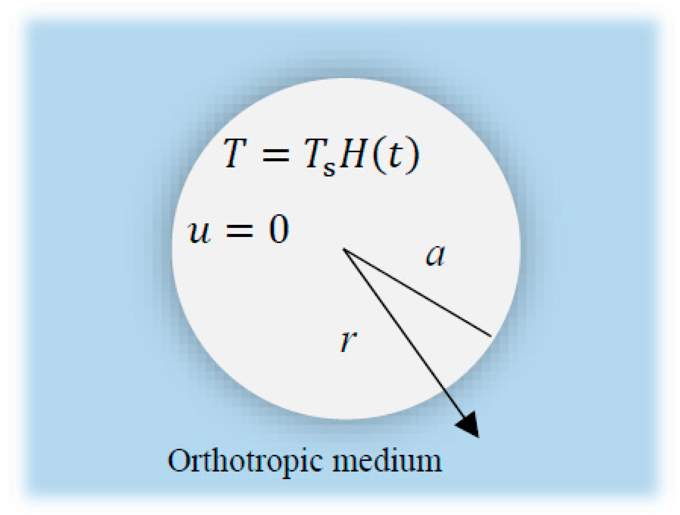
The basic equations in an orthotropic material in the absence of body forces and thermal source are presented as [2]:

$${\sigma }_{ij,j}=\rho \frac{{\partial }^2{u}_i}{\partial t^2},$$

(1)

$$\frac{\partial T_{,ii}}{\partial t}{\left(K_{ii}{T}_{,i}\right)}_{,i}=\left(\frac{\partial }{\partial t}+{\tau }_o\frac{{\partial }^2}{\partial t^2}\right) \left(\rho c_{e}T+{\beta }_{ii}{T}_o\partial u_{j,j}\right),$$

(2)

$${\sigma }_{ij}=c_{ijkl}{e}_{kl }-{\beta }_{ij}\left(T-T_o\right){\delta }_{ij},$$

(3)

$$e_{ij}=\frac{1}{2}\left(u_{i,j}+u_{j,i}\right),$$

(4)

where $T$ points to the temperature increments, $c_e$ points to the specific heat, ${\beta }_{ij}$ are the thermal moduli, $\rho$ is the density of mass, $K_{ii}$ are the thermal conductivity components that are temperature-dependent and variable, $e_{kl}$ are the strain tensor components and $c_{ijkl}$ are the elastic constants, $T_o$ is the reference temperature, ${\sigma }_{ij}$ are the stresses components and $u_i$ are the components of displacement. Consider an unbounded elastic body involving spherical cavities occupying the area $a \le r<\infty$, whose states are defined in terms of space variable $r$ and the time variable $t$. The only non-vanishing component of displacement is the radial one $u_r=u\left(r,t\right)$, which is related to the spherical coordinates $\left(r,\theta ,\phi \right)$ as in Figure 1. The nonvanishing strain tensor components are as follows:

$$e_{rr}=\frac{\partial u}{\partial r},e_{\theta \theta }= \frac{u}{r},e_{\phi \phi }=\frac{u}{r},$$

(5)

Substituting for $e_{rr}$, $e_{\theta \theta }$ and $e_{\phi \phi }$ into the basic equations can be given by

$$\frac{\partial {\sigma }_{rr}}{\partial r}+\frac{1}{r}\left(2{\sigma }_{rr}-{\sigma }_{\theta \theta }-{\sigma }_{\phi \phi }\right)=\rho \frac{{\partial }^{2}u}{\partial t^2},$$

(6)

$$\frac{1}{r^2}\frac{\partial }{\partial r}\left(r^{2}K\left(T\right)\frac{\partial T}{\partial r}\right)=\left(\frac{\partial }{\partial t}+{\tau }_o\frac{{\partial }^2}{\partial t^2}\right)\left(\rho c_{e}T+{\beta }_{11}{T}_o\frac{\partial u}{\partial r}+{\beta }_{22}{T}_o\frac{2u}{r}\right),$$

(7)

$$\begin{gathered} {\sigma }_{rr}=c_{11}\frac{\partial u}{\partial r}+c_{12}\frac{2u}{r}-{\beta }_{11}T, \\ {\sigma }_{\theta \theta }={\sigma }_{\phi \phi }=c_{12}\frac{\partial u}{\partial r}+\left(c_{22}+c_{23}\right)\frac{u}{r}-{\beta }_{22}T, \end{gathered}$$

(8)

$$e=\frac{\partial u}{\partial r}+\frac{2u}{r},$$

(9)

In this case, the varying thermal conductivity of orthotropic media that may be chosen as in [52]

$$K\left(T\right)=K_o\left(1+K_{n}T\right),$$

(10)

where $K_o$ are the thermal conductivity when $T=T_o$ and $K_n\le 0$ identifies the negative parameter.

3. Application

The initial condition can be given by:

$$u\left(r,0\right)=0, \frac{\partial u\left(r,0\right)}{\partial t}=0, T\left(r,0\right)=0, \frac{\partial T\left(r,0\right)}{\partial t}=0,$$

(11)

whereas the following constitute the requirements of the boundaries:

$$u\left(a,t\right)=0, T\left(a,t\right)=T_{s}H\left(t\right),$$

(12)

where $H\left(t\right)$ is the Heaviside function and $T_s$ is constant. Consequently, the nondimensionality of variables may be stated as follows:

$$T^{*}=\frac{ T-T_o}{T_o}, \left(r^{*},u^{*}\right)=\mu c\left(r,u\right), \left(t^{*},{\tau }_o^{*}\right)=\omega c^2\left(t,{\tau }_o\right), \left({\sigma }_{rr}^{*},{\sigma }_{\theta \theta }^{*}\right)=\frac{ \left({\sigma }_{rr},{\sigma }_{\theta \theta },\right)}{c_{11}},$$

(13)

where $\mu =\frac{\rho c_e}{K_o}$ and $c=\sqrt{\frac{c_{11}}{\mathsf{\rho }}}$. Equation (13)’s non-dimensional governing equations are written as (after the superscript * has been removed for appropriateness)

$$\frac{{\partial }^{2}u}{\partial r^2}+\frac{2}{r}\frac{\partial u}{\partial r}-\frac{2\left(s_3-s_1\right)u}{r^2}-s_2\frac{\partial T}{\partial r}+\frac{2\left(s_4-s_2\right)}{r}T=\frac{{\partial }^{2}u}{ \partial t^2},$$

(14)

$$\left(1+K_{n}T\right)\frac{{\partial }^{2}T}{\partial r^2}+K_n{\left(\frac{\partial T}{\partial r}\right)}^2+ \frac{2\left(1+K_{n}T\right)}{r}\frac{\partial T}{\partial r}=\left(\frac{\partial }{\partial t}+{\tau }_o\frac{{\partial }^2}{\partial t^2}\right)\left(T+{\epsilon }_1\frac{\partial u}{\partial r}+{\epsilon }_2\frac{2u}{r}\right),$$

(15)

$$\begin{gathered} {\sigma }_{rr}=\frac{\partial u}{\partial r}+2s_1\frac{u}{r}-s_{2}T, \\ {\sigma }_{\theta \theta }={\sigma }_{\phi \phi }=s_1\frac{\partial u}{\partial r}+s_3\frac{u}{r}-s_{4}T, \end{gathered}$$

(16)

where $s_1=\frac{c_{12}}{c_{11}}$, $s_2=\frac{T_o{\beta }_{11}}{c_{11}}$, $s_3=\frac{\left(c_{22}+c_{23}\right)}{c_{11}}$, $s_4=\frac{T_o{\beta }_{22}}{c_{11}}$, ${\epsilon }_1=\frac{{\beta }_{11}}{\rho c_e}$, ${\epsilon }_2=\frac{{\beta }_{22}}{\rho c_e}$.

4. Numerical Scheme

The standard techniques may be used to generate the finite element method (FEM) for thermoelasticity problems. The finite element scheme is the preferred method for complex systems in numerous domains since it is a powerful and most sophisticated way to obtain numerical solutions to complicated problems. The solutions of the governing relations (14) and (15) under the boundary condition (12) and the use of the initial condition (11) are obtained using a finite element diagram. The displacement $u$ and the temperature $T$ are linked to the corresponding nodal values in finite element techniques by

$$u={{\displaystyle \sum }}_{j=1}^n{N}_j{u}_j\left(t\right),T={{\displaystyle \sum }}_{j=1}^n{N}_j{T}_j\left(t\right),$$

(17)

where $n$ refers to the number of nodes per element, and $N$ refers to the shape functions. For the unknown displacement $u$ and the unknown temperature $T$, the same shape function is used in Galerkin methods to approximate the corresponding test functions.

$$\delta u={{\displaystyle \sum }}_{j=1}^n{N}_j\delta u_j, \delta T={{\displaystyle \sum }}_{j=1}^n{N}_j\delta T_j,$$

(18)

We assume that the master elements local coordinates fall between [1 and −1]. In this situation, one-dimension quadratic components are used, and they are written as follows:

$$\begin{array}{ccc}{N}_1=\frac{1}{2}\left({\chi }^2+\chi \right),& N_1=1-{\chi }^2,& N_3=\frac{1}{2}\left({\chi }^{2 }-\chi \right)\end{array},$$

(19)

The weak formulation of finite element method that correspond to the nonlinear formulations (14) and (15) may be written by:

$${{\displaystyle \int }}_a^L\delta u\left(\frac{{\partial }^{2}u}{\partial t^2}-\frac{2}{r}\frac{\partial u}{\partial r}+\frac{2\left(s_3-s_1\right)u}{r^2}+s_2\frac{\partial T}{\partial r}-\frac{2\left(s_4-s_2\right)}{r}T\right)dr+{{\displaystyle \int }}_a^L\frac{\partial \delta u}{\partial r}\left(\frac{\partial u}{\partial r}\right)dr=\delta u{\left(\frac{\partial u}{\partial r}\right)}_a^L,$$

(20)

$${{\displaystyle \int }}_a^L\delta T\left((\frac{\partial }{\partial t}+{\tau }_o\frac{{\partial }^2}{\partial t^2})(T+{\epsilon }_1\frac{\partial u}{\partial r}+{\epsilon }_2\frac{2u}{r})-\frac{2\left(1+K_{n}T\right)}{r}\frac{\partial T}{\partial r}\right)dr+{{\displaystyle \int }}_a^L\frac{\partial \delta T}{\partial r}\left(\left(1+K_{n}T\right)\frac{\partial T}{\partial r}\right)dr=\delta T{\left(\left(1+K_{n}T\right)\frac{\partial T}{\partial r}\right)}_a^L.$$

(21)

Implicit approaches can be employed to determine the time derivatives of unknown variables. For example, the time derivatives of the unknown variables must be determined using the Newmark time integration method or the central finite difference method by time step $0.0001$ [53]. The grid size was changed until the values of the fields under examination were stable. Further increasing the mesh size over 25,000 elements has no discernible effect on the results. Therefore, for this investigation, a grid size of 25,000 was chosen.

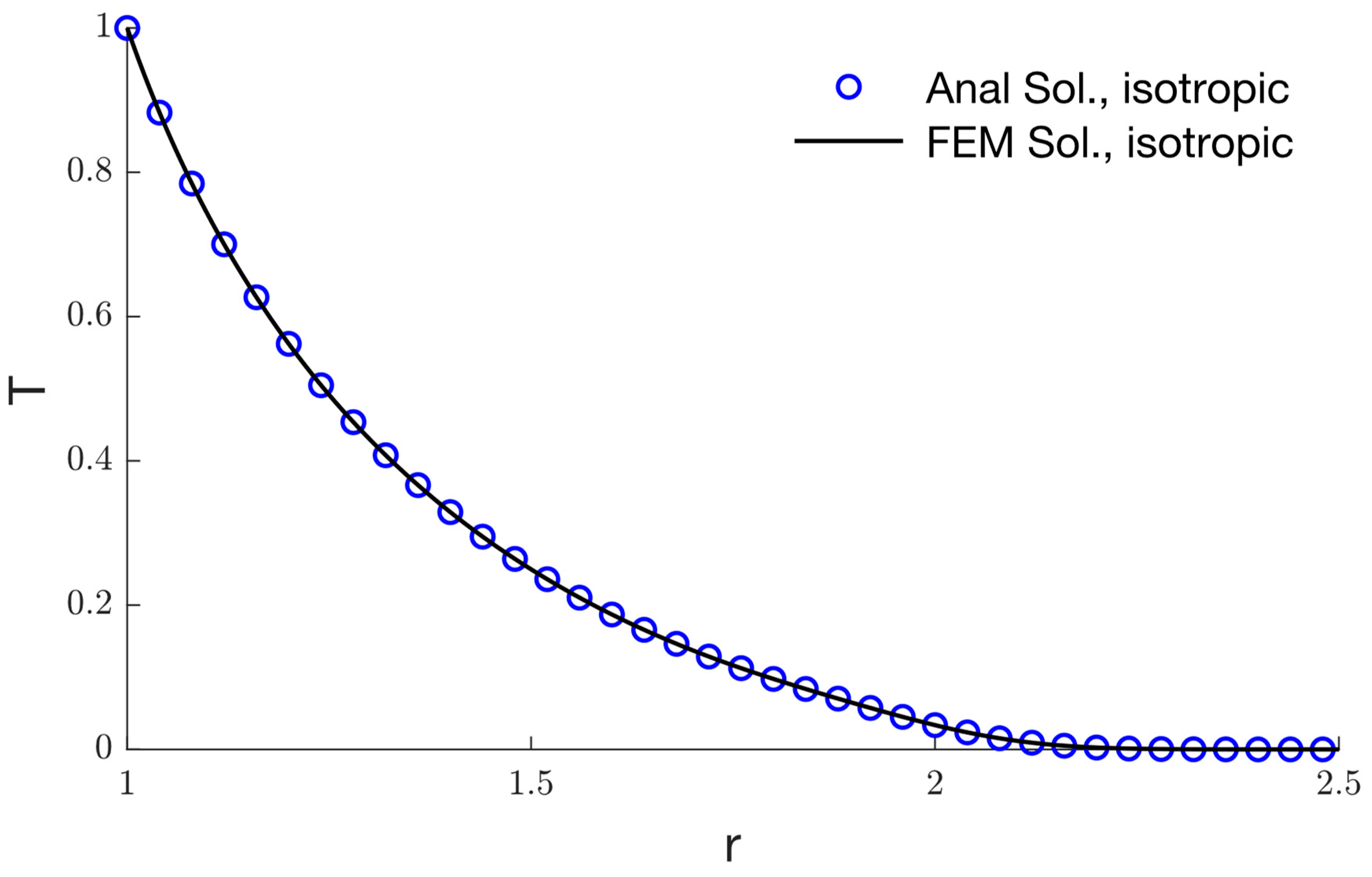
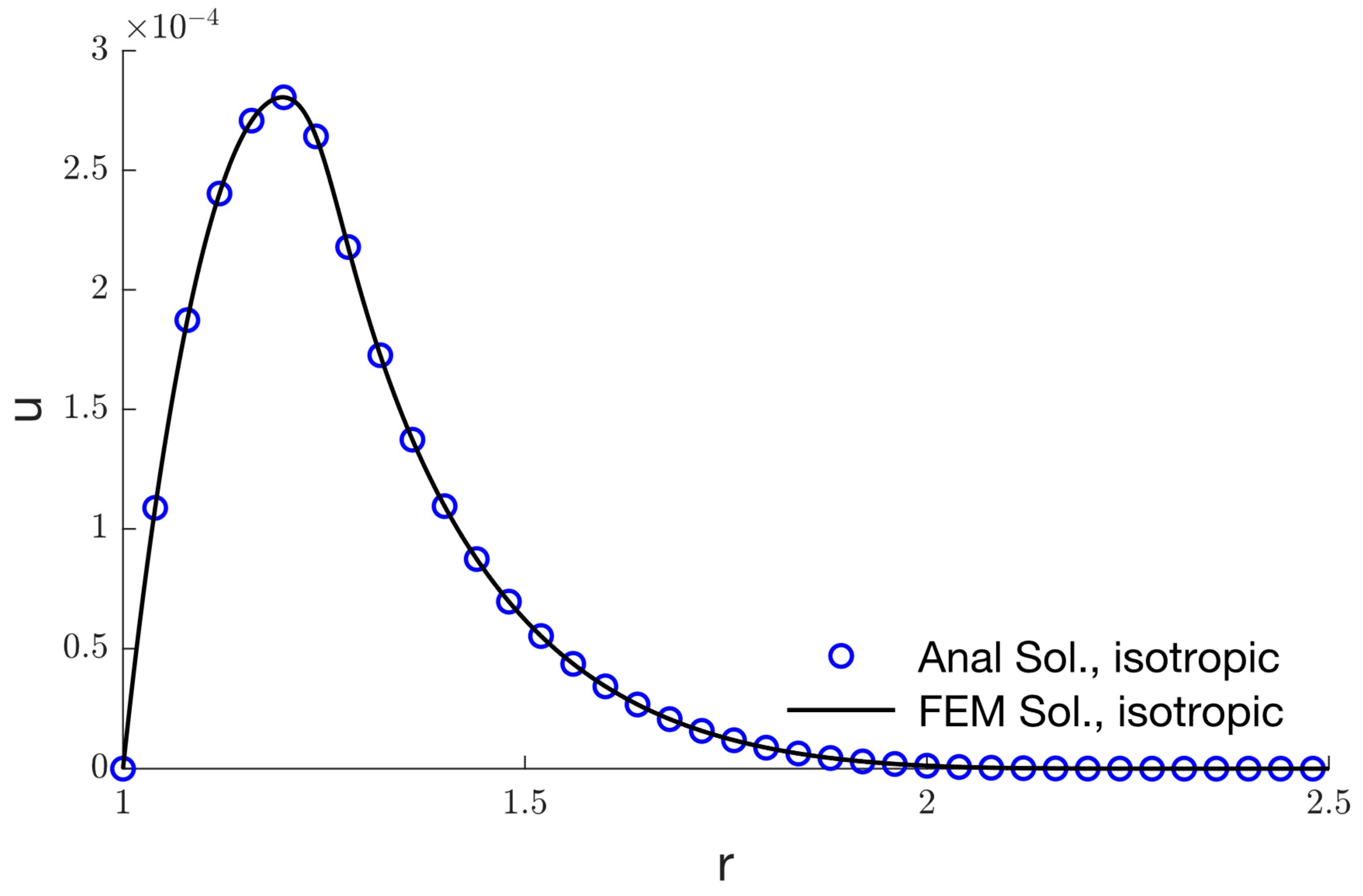
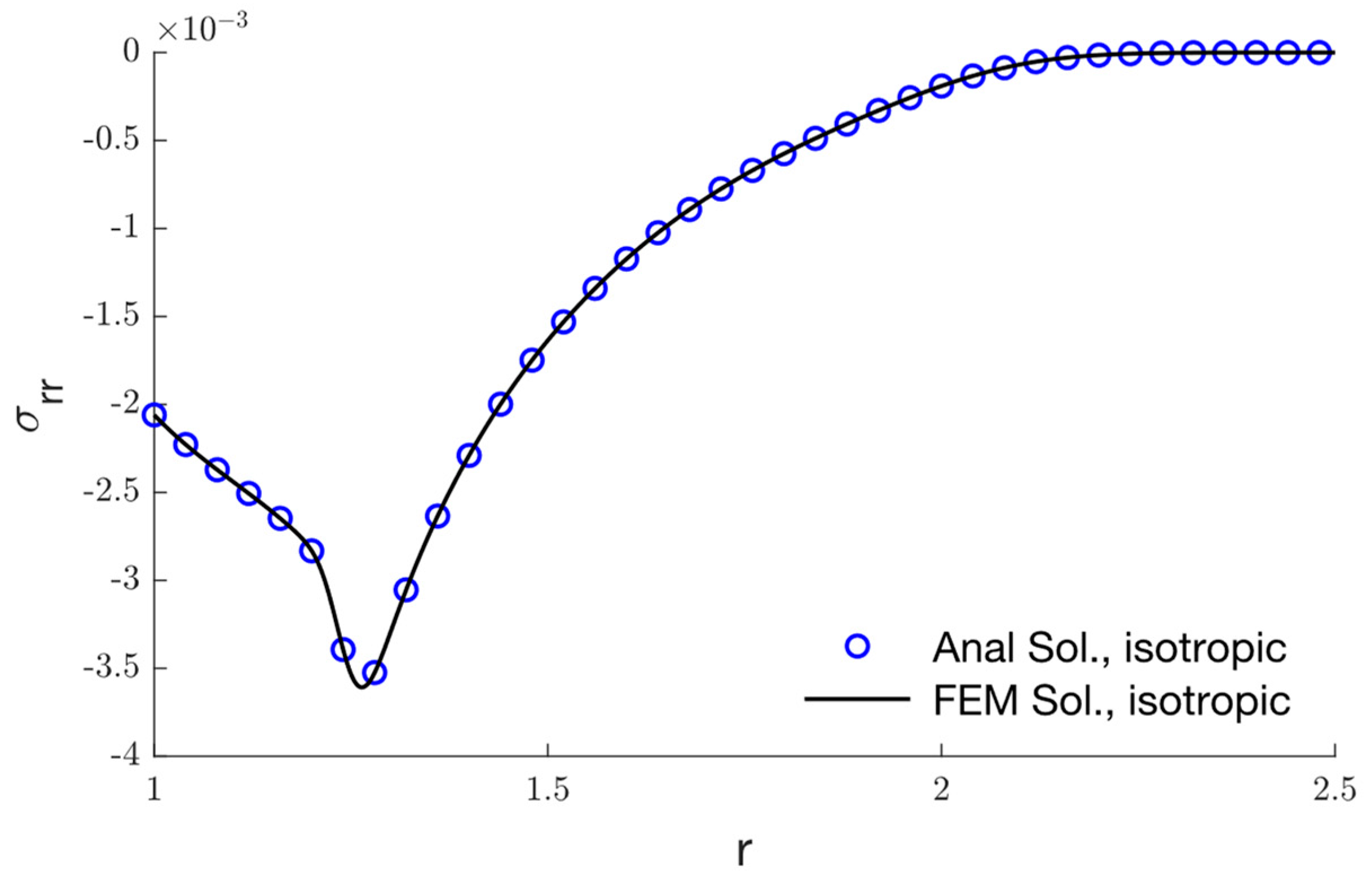
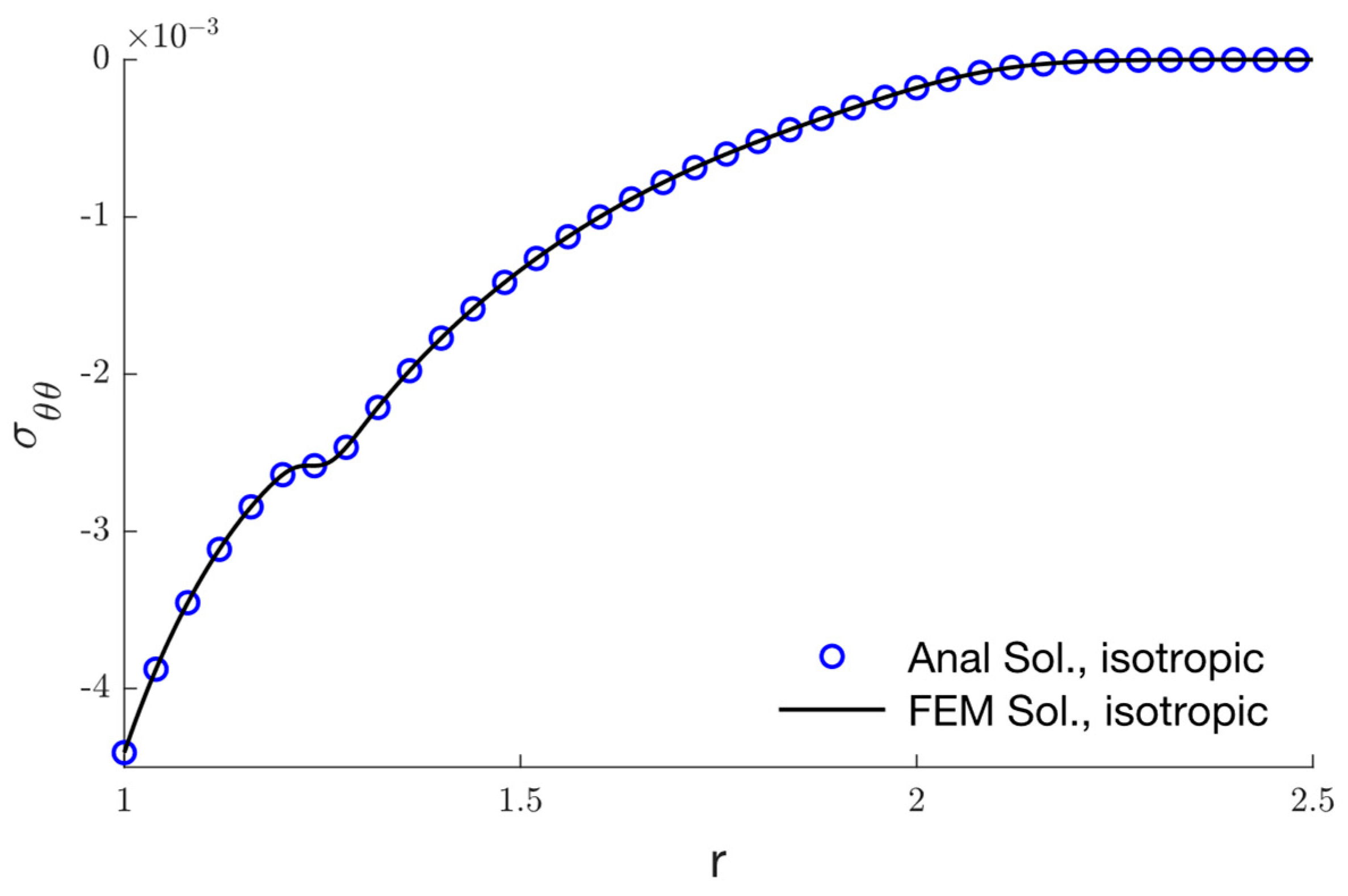
5. Special Cases and the Validation of the Numerical Approach

Analytical solutions for homogeneous and isotropic material are being provided to validate the finite element approach. Moreover, when $K_n=0$, the analytical and numerical solutions are compared with each other to validate the numerical solutions. For homogeneous and isotropic material $c_{11}=c_{22}=\lambda +2\mu ,c_{12}=c_{23}=\lambda ,{\beta }_{11}={\beta }_{22}=\gamma$ and $K_n=0$. As a consequence of this, Equations (14)–(16) with the initial and boundary conditions may be expressed as follows:

$$\frac{{\partial }^{2}u}{\partial r^2}+\frac{2}{r}\frac{\partial u}{\partial r}-\frac{2u}{r^2}-a_2\frac{\partial T}{\partial r}=\frac{{\partial }^{2}u}{\partial t^2},$$

(22)

$$\frac{{\partial }^{2}T}{\partial r^2}+ \frac{2}{r}\frac{\partial T}{\partial r}=\left(\frac{\partial }{\partial t}+{\tau }_o\frac{{\partial }^2}{\partial t^2}\right)\left(T+{\epsilon }_1\left(\frac{\partial u}{\partial r}+\frac{2u}{r}\right)\right),$$

(23)

$$\begin{gathered} {\sigma }_{rr}=\frac{\partial u}{\partial r}+2a_1\frac{u}{r}-a_{2}T, \\ {\sigma }_{\theta \theta }={\sigma }_{\phi \phi }=a_1\frac{\partial u}{\partial r}+\left(1+a_1\right)\frac{u}{r}-a_{2}T, \end{gathered}$$

(24)

$$u\left(r,0\right)=0,\frac{\partial u\left(r,0\right)}{\partial t}=0,T\left(r,0\right)=0,\frac{\partial T\left(r,0\right)}{\partial t}=0,$$

(25)

$$T\left(a,t\right)=T_{s}H\left(t\right), u\left(a,t\right)=0,$$

(26)

where $a_1=\frac{\lambda }{\lambda +2\mu }$, $a_2=\frac{T_o\gamma }{\lambda +2\mu }$, $\epsilon =\frac{\gamma }{\rho c_e}$. Applying Laplace transforms in order to find solutions to Equations (22)–(26):

$$\overline{f}\left(x,s\right)=L\left[f\left(x,t\right)\right]=\underset{0}{\overset{\infty }{{\displaystyle \int }}}f\left(x,t\right)e^{-st}dt.$$

(27)

As a consequence of this, we can deduce the following:

$$\frac{d^2\overline{u}}{d{r}^2}+\frac{2}{r}\frac{d\overline{u}}{dr}-\frac{2\overline{u}}{r^2}=s^2\overline{u}+a_2\frac{d\overline{T}}{dr},$$

(28)

$$\frac{d^2\overline{T}}{d{r}^2}+ \frac{2}{r}\frac{d\overline{T}}{dr}=\left(s+s^2{\tau }_o\right)\left(\overline{T}+{\epsilon }_1\left(\frac{d\overline{u}}{dr}+\frac{2\overline{u}}{r}\right)\right),$$

(29)

$$\begin{gathered} {\overline{\sigma }}_{rr}=\frac{d\overline{u}}{dr}+2a_1\frac{\overline{u}}{r}-a_2\overline{T}, \\ {\overline{\sigma }}_{\theta \theta }={\overline{\sigma }}_{\phi \phi }=a_1\frac{d\overline{u}}{dr}+\left(1+a_1\right)\frac{\overline{u}}{r}-a_2\overline{T}, \end{gathered}$$

(30)

$$\overline{T}\left(a,s\right)=\frac{T_s}{s},\overline{u}\left(a,s\right)=0,$$

(31)

Using Equation (28) with the differentiating Equation (29) with respect to $r$, we obtain

$$\frac{d^2}{d{r}^2}\left(\frac{d\overline{T}}{dr}\right)+ \frac{2}{r}\frac{d}{dr}\left(\frac{d\overline{T}}{dr}\right)-\frac{2}{r^2}\left(\frac{d\overline{T}}{dr}\right)=\left(s+s^2{\tau }_o\right)\left({\epsilon }_1{s}^2\overline{u}+\left(1+a_2{\epsilon }_1\right)\frac{d\overline{T}}{dr}\right)$$

(32)

It is possible to write Equations (28) and (32) in the form of a vector–matrix differential equation as follows:

$$DV=AV,$$

(33)

where $\frac{d^2}{d{r}^2}+\frac{2}{r}\frac{d}{dr}-\frac{2}{r^2}$, $V={\left(\begin{array}{cc}\overline{u}& \frac{d\overline{T}}{dr}\end{array}\right)}^T$ and $A=\left(\begin{array}{cc}{a}_{11}& a_{12}\\ a_{21}& a_{22}\end{array}\right)$, $a_{11}=s^2$, $a_{12}=a_2$, $a_{21}={\epsilon }_1{s}^2\left(s+s^2{\tau }_o\right)$ and $a_{22}=\left(1+a_2{\epsilon }_1\right)\left(s+s^2{\tau }_o\right)$,

The using of eigenvalue approach [54,55] to solve the Equation (33), the characteristic relation of matrix $A$ can be written as

$$a_{11}{a}_{22}-a_{12}{a}_{21}-\left(a_{11}+a_{22}\right)\zeta +{\zeta }^2=0,$$

(34)

where $\zeta ={\zeta }_1$, $\zeta$=${\zeta }_2$ are the roots of the characteristic Equation (34) which have the corresponding eigenvectors $X_1=a_{12}$ and $X_2=\zeta -a_{11}$. Thus, the solution of Equation (34) can be expressed by

$$\overline{u}\left(r,s\right)=r^{-1/2}{U}_1{A}_1{I}_{3/2}\left(r\sqrt{{\zeta }_1}\right)+r^{-1/2}{U}_2{A}_2{I}_{3/2}\left(r\sqrt{{\zeta }_2}\right),$$

(35)

$$\overline{T}\left(r,s\right)=\frac{T_1}{\sqrt{r{\zeta }_1}}{A}_1{I}_{1/2}\left(r\sqrt{{\zeta }_1}\right)+\frac{T_2}{\sqrt{r{\zeta }_2}}{A}_2{I}_{1/2}\left(r\sqrt{{\zeta }_2}\right)$$

(36)

where $A_1$ and $A_2$ are constants that can be calculated from the boundary condition of the problem, and $I_{3/2},I_{1/2}$ are the modified of Bessel’s functions with order $\frac{3}{2}$ and $\frac{1}{2,}$ respectively. It is possible to use the Stehfest [56] method as a numerical inversion technique in order to obtain the final solutions of temperature, displacement and stresses distributions.

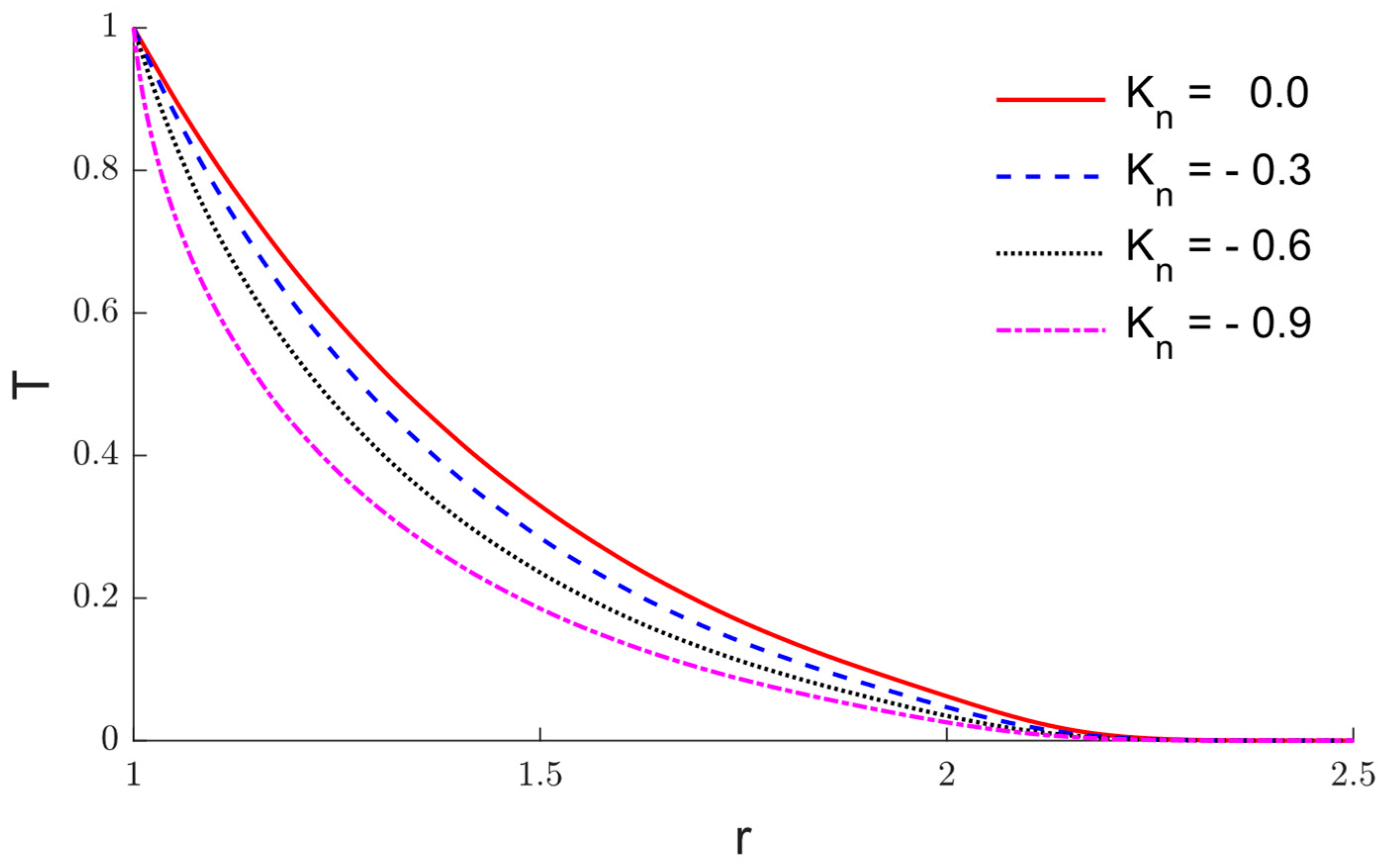
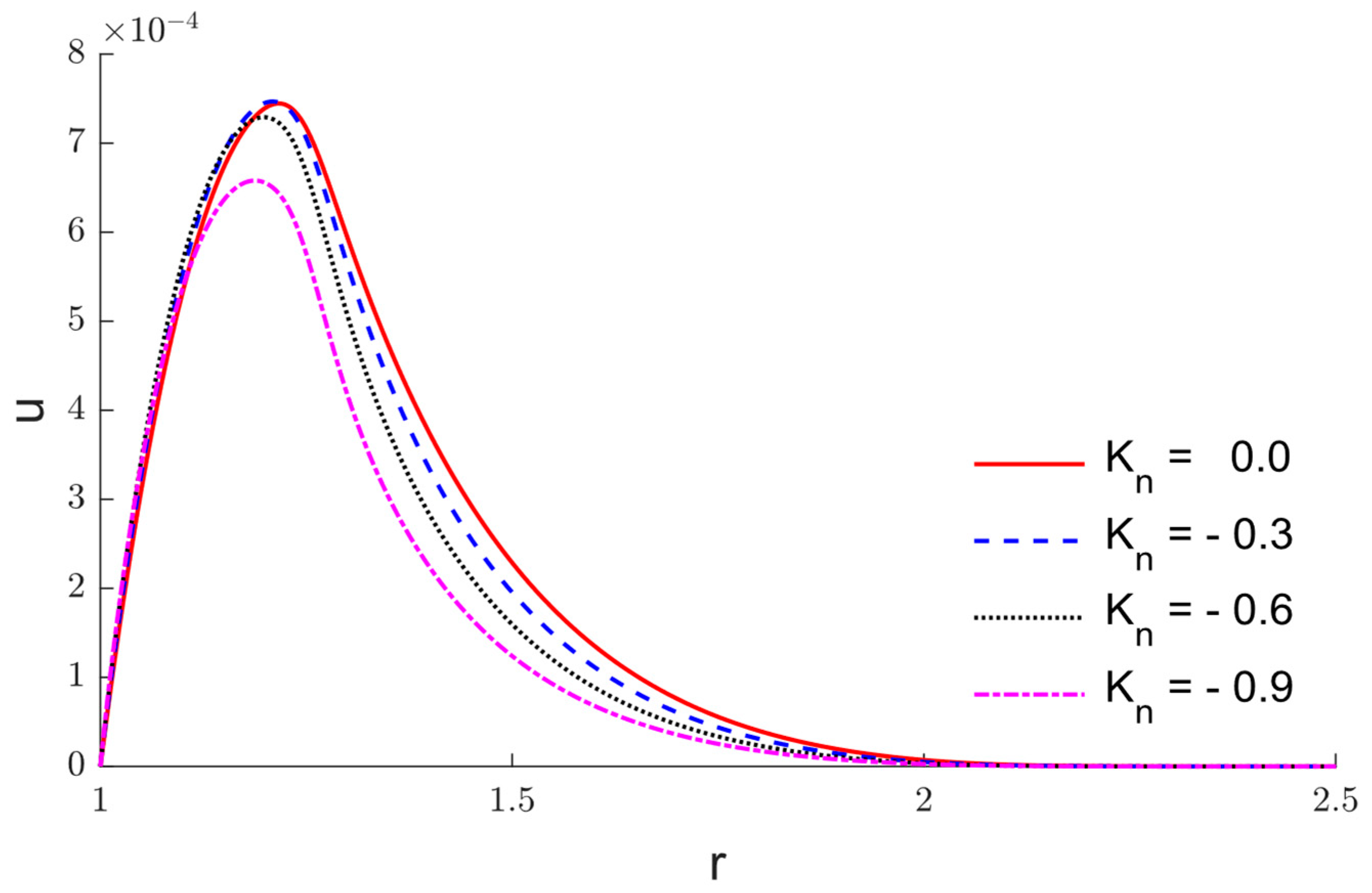
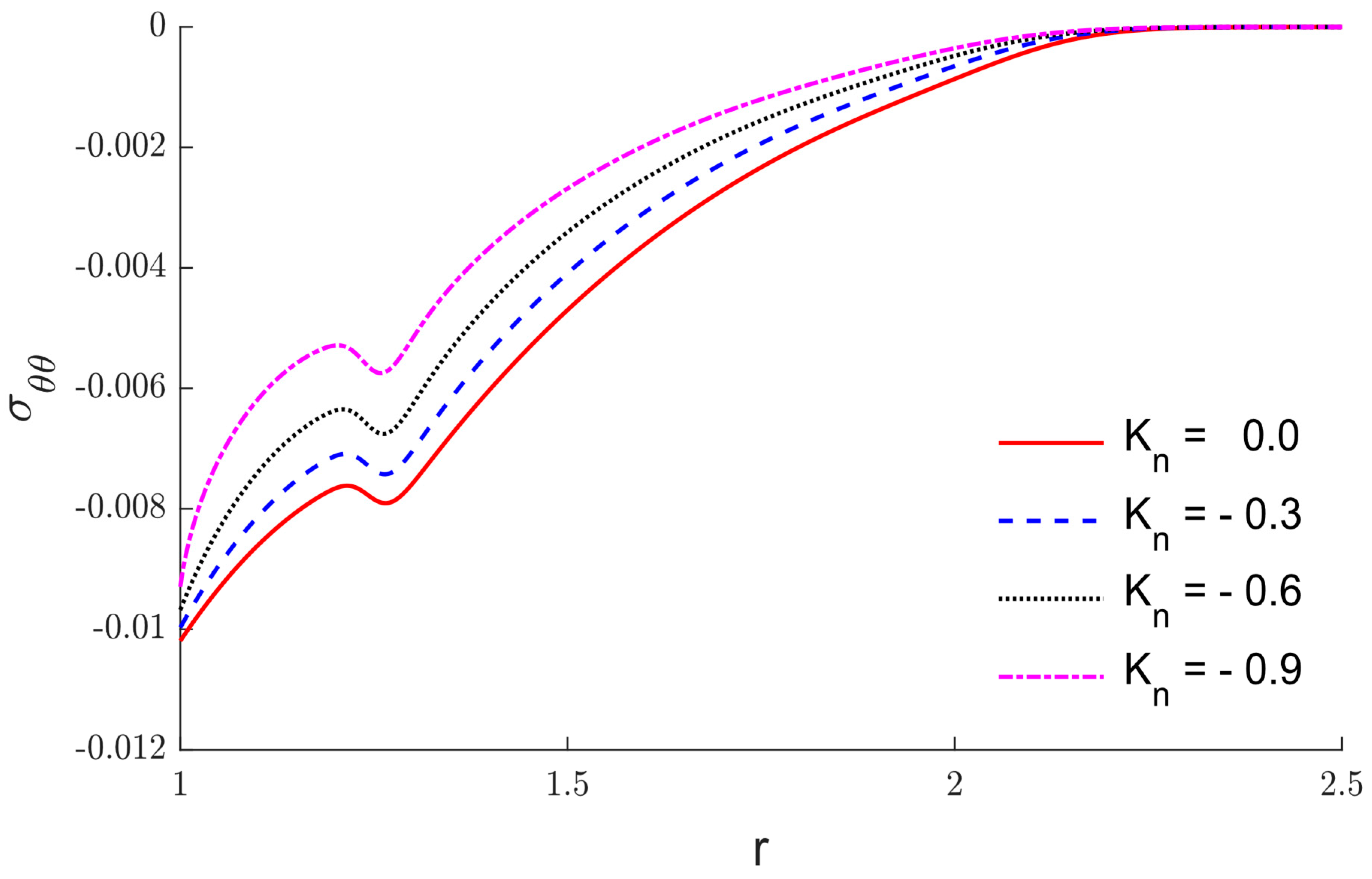
6. Numerical Outcomes and Discussions

Numerical results for a single crystal of magnesium medium using the following physical parameters are computed to demonstrate the theoretical findings derived in the previous sections [57]:

$$\begin{gathered} c_{11}=5.974\times {10}^{10}\left(\mathrm{N}\right)\left({\mathrm{m}}^{-2}\right),{\beta }_{11}={\beta }_{22}=2.68\times {10}^6\left(\mathrm{N}\right) \left({\mathrm{m}}^{-2}\right)\left({\mathrm{k}}^{-1}\right),T_o=298\left(k\right),a=1, \\ {c}_{22}=6.17\times {10}^{10}\left(\mathrm{N}\right) \left({\mathrm{m}}^{-2}\right), K_o=170 \left(\mathrm{W}\right)\left({\mathrm{m}}^{-1}\right)\left({\mathrm{k}}^{-1}\right),c_{12}=2.624\times {10}^{10}\left(\mathrm{N}\right)\left({\mathrm{m}}^{-2}\right), \\ \rho =1470\left(\mathrm{k}\mathrm{g}\right)\left({\mathrm{m}}^{-3}\right), c_e=1040 \left(\mathrm{J}\right)\left(\mathrm{k}{\mathrm{g}}^{-1}\right)\left({\mathrm{k}}^{-1}\right),{\tau }_o=0.05,t=0.25, \\ {c}_{23}=2.17\times {10}^{10}\left(\mathrm{N}\right)\left({\mathrm{m}}^{-2}\right). \end{gathered}$$

Figure 2, Figure 3, Figure 4, Figure 5, Figure 6, Figure 7, Figure 8, Figure 9, Figure 10, Figure 11, Figure 12, Figure 13, Figure 14, Figure 15, Figure 16, Figure 17, Figure 18, Figure 19, Figure 20 and Figure 21 show the calculated physical values (numerical) under generalized thermoelastic theory with one thermal delay time based on the previous set of parameters. The computation is carried out for the time $t=0.25$. The temperature variations, radial displacement, and the variation in the radial and shear stress distributions along the radial distances $r$ under variable thermal conductivity are determined numerically. Figure 2 shows the variation in temperature along the radial distance $r$. It is clear that the temperature has maximums value $T=1$ at the internal surface of hole $a=1$ to accept the boundary condition of the problem, and then steadily falls when the radial distance $r$ is increased to close to zero. Figure 3 shows the variations in radial displacement via the radial distances. It is seen that the radial displacement starts at zero, which meets the boundary condition of the problem, and lowers steadily up to peak values before decreasing to near zero. Figure 4 depicts the variations of radial stress ${\sigma }_{rr}$ versus the radial distances $r$. The radial stress has maximum negative values before gradually diminishing to near zero. The variations in shear stress ${\sigma }_{\theta \theta }$ along the radial distance $r$ are displayed in Figure 5. It is noted that it has negative maximums before steadily rising to zero. Under the variable thermal conductivity, there are big significant variances in the values of all considering variables, according to the results. The varying thermal conductivity has a remarkable impact on the values of all considering variables, as predicted. Figure 6, Figure 7, Figure 8 and Figure 9 show the impact of thermal delay time in all physical quantities, whereas Figure 10, Figure 11, Figure 12 and Figure 13 show the variation of physical quintettes along the distance for different time values. The variations in temperature, the radial displacement, the radial stress and the shear stress under comparisons between the isotropic and orthotropic materials under varying thermal conductivity and with one relaxation time are shown in Figure 14, Figure 15, Figure 16 and Figure 17. The analytical results for isotropic elastic material have been presented to verify that the suggested approach is accurate as in Figure 14, Figure 15, Figure 16 and Figure 17. Additionally, the variations of temperature, the radial displacement, the radial stress and the shear stress under the comparisons between the elastic and orthotropic materials under varying thermal conductivity and with one relaxation time are shown in Figure 18, Figure 19, Figure 20 and Figure 21. Finally, based on the numerical results, it is possible to infer that utilizing a generalized thermoelastic theory under the changing thermal conductivity is a major phenomenon with a considerable effect on the physical quantity distributions.

7. Conclusions

This work presents a mathematical analysis of the effect of variable thermal conductivity in an orthotropic medium including a spherical hole. The distributions of temperature, radial displacement, radial stress, and shear stress in a thermoelastic orthotropic medium with one thermal relaxation time have been given. To provide a numerical solution for nonlinear equations, the finite element technique is used. It was discovered that the varying thermal conductivity has significant effects and influences how various physical field components behave as they deform. The effects of thermal delay time are presented. It was shown that the deformation behaviour of different components of physical fields is significantly affected by the thermal relaxation time. The impact of time is shown. It was shown that time has a considerable impact on the deformation behavior of several physical field components. There are comparisons shown between the orthotropic and isotropic materials. To verify that the suggested approach is accurate, numerical solutions and analytical solutions have been compared for isotropic elastic material.

References

1. Lord, H.W.; Shulman, Y. A generalized dynamical theory of thermoelasticity. J. Mech. Phys. Solids 1967, 15, 299–309. [Google Scholar] [CrossRef]
2. Dhaliwal, R.S.; Sherief, H.H. Generalized thermoelasticity for anisotropic media. Q. Appl. Math. 1980, 38, 1–8. [Google Scholar] [CrossRef]
3. Hetnarski, R.B. Thermal Stresses IV; Elsevier: Amsterdam, The Netherlands, 1996. [Google Scholar]
4. Sherief, H.; Abd El-Latief, A.M. Effect of variable thermal conductivity on a half-space under the fractional order theory of thermoelasticity. Int. J. Mech. Sci. 2013, 74, 185–189. [Google Scholar] [CrossRef]
5. Mukhopadhyay, S.; Kumar, R. Solution of a Problem of Generalized Thermoelasticity of an Annular Cylinder with Variable Material Properties by Finite Difference Method. Comput. Methods Sci. Technol. 2009, 15, 169–176. [Google Scholar] [CrossRef]
6. Abo-Dahab, S.M.; Abbas, I.A. LS model on thermal shock problem of generalized magneto-thermoelasticity for an infinitely long annular cylinder with variable thermal conductivity. Appl. Math. Model. 2011, 35, 3759–3768. [Google Scholar] [CrossRef]
7. Abbas, I.A.; Abd-Alla, A.-E.N. Effects of thermal relaxations on thermoelastic interactions in an infinite orthotropic elastic medium with a cylindrical cavity. Arch. Appl. Mech. 2007, 78, 283–293. [Google Scholar] [CrossRef]
8. Yasein, M.d.; Mabrouk, N.; Lotfy, K.; EL-Bary, A. The influence of variable thermal conductivity of semiconductor elastic medium during photothermal excitation subjected to thermal ramp type. Results Phys. 2019, 15, 102766. [Google Scholar] [CrossRef]
9. Zenkour, A.M.; Abbas, I.A. Magneto-thermoelastic response of an infinite functionally graded cylinder using the finite element method. J. Vib. Control 2013, 20, 1907–1919. [Google Scholar] [CrossRef]
10. Sharma, P.K.; Bajpai, A.; Kumar, R. Analysis of two temperature thermoelastic diffusion plate with variable thermal conductivity and diffusivity. Waves Random Complex Media 2021, 1–19. [Google Scholar] [CrossRef]
11. Hobiny, A.; Abbas, I. Generalized thermoelastic interaction in a two-dimensional orthotropic material caused by a pulse heat flux. Waves Random Complex Media 2021, 1–18. [Google Scholar] [CrossRef]
12. Song, Y.; Todorovic, D.M.; Cretin, B.; Vairac, P. Study on the generalized thermoelastic vibration of the optically excited semiconducting microcantilevers. Int. J. Solids Struct. 2010, 47, 1871–1875. [Google Scholar] [CrossRef]
13. Mondal, S.; Sur, A. Photo-thermo-elastic wave propagation in an orthotropic semiconductor with a spherical cavity and memory responses. Waves Random Complex Media 2020, 31, 1835–1858. [Google Scholar] [CrossRef]
14. Said, S.M. Eigenvalue approach on a problem of magneto-thermoelastic rotating medium with variable thermal conductivity: Comparisons of three theories. Waves Random Complex Media 2021, 31, 1322–1339. [Google Scholar] [CrossRef]
15. Lata, P.; Himanshi. Fractional effect in an orthotropic magneto-thermoelastic rotating solid of type GN-II due to normal force. Struct. Eng. Mech. 2022, 81, 503–511. [Google Scholar] [CrossRef]
16. Singh, B.; Pal, S. Magneto-thermoelastic interaction with memory response due to laser pulse under Green-Naghdi theory in an orthotropic medium. Mech. Based Des. Struct. Mach. 2020, 50, 3105–3122. [Google Scholar] [CrossRef]
17. Hobiny, A.; Abbas, I.A. Analytical solutions of photo-thermo-elastic waves in a non-homogenous semiconducting material. Results Phys. 2018, 10, 385–390. [Google Scholar] [CrossRef]
18. Zenkour, A.M.; Abbas, I.A. Nonlinear Transient Thermal Stress Analysis of Temperature-Dependent Hollow Cylinders Using a Finite Element Model. Int. J. Struct. Stab. Dyn. 2014, 14, 1450025. [Google Scholar] [CrossRef]
19. Vlase, S.; Marin, M.; Öchsner, A.; Scutaru, M.L. Motion equation for a flexible one-dimensional element used in the dynamical analysis of a multibody system. Contin. Mech. Thermodyn. 2018, 31, 715–724. [Google Scholar] [CrossRef]
20. Marin, M.; Vlase, S.; Paun, M. Considerations on double porosity structure for micropolar bodies. AIP Adv. 2015, 5, 037113. [Google Scholar] [CrossRef]
21. Marin, M. An evolutionary equation in thermoelasticity of dipolar bodies. J. Math. Phys. 1999, 40, 1391–1399. [Google Scholar] [CrossRef]
22. Lata, P.; Singh, S. Stoneley wave propagation in nonlocal isotropic magneto-thermoelastic solid with multi-dual-phase lag heat transfer. Steel Compos. Struct. 2021, 38, 141–150. [Google Scholar] [CrossRef]
23. Kaur, H.; Lata, P. Effect of thermal conductivity on isotropic modified couple stress thermoelastic medium with two temperatures. Steel Compos. Struct. 2020, 34, 309–319. [Google Scholar] [CrossRef]
24. Lata, P.; Kumar, R.; Sharma, N. Plane waves in an anisotropic thermoelastic. Steel Compos. Struct. 2016, 22, 567–587. [Google Scholar] [CrossRef]
25. Lataa, P.; Kaur, I. Effect of time harmonic sources on transversely isotropic thermoelastic thin circular plate. Geomach. Eng. 2019, 19, 29–36. [Google Scholar] [CrossRef]
26. Marin, M.; Baleanu, D.; Vlase, S. Effect of microtemperatures for micropolar thermoelastic bodies. Struct. Eng. Mech. 2017, 61, 381–387. [Google Scholar] [CrossRef]
27. Abbas, I.A.; Alzahrani, F.S.; Elaiw, A. A DPL model of photothermal interaction in a semiconductor material. Waves Random Complex Media 2018, 29, 328–343. [Google Scholar] [CrossRef]
28. Abbas, I.A. Eigenvalue approach on fractional order theory of thermoelastic diffusion problem for an infinite elastic medium with a spherical cavity. Appl. Math. Model. 2015, 39, 6196–6206. [Google Scholar] [CrossRef]
29. Lata, P.; Himanshi. Orthotropic magneto-thermoelastic solid with higher order dual-phase-lag model in frequency domain. Struct. Eng. Mech. 2021, 77, 315–327. [Google Scholar] [CrossRef]
30. Hobiny, A.; Abbas, I.A. A GN model of thermoelastic interaction in a 2D orthotropic material due to pulse heat flux. Struct. Eng. Mech. 2021, 80, 669–675. [Google Scholar] [CrossRef]
31. Said, S.M.; Othman, M.I.A. The effect of gravity and hydrostatic initial stress with variable thermal conductivity on a magneto-fiber-reinforced. Struct. Eng. Mech. 2020, 74, 425–434. [Google Scholar] [CrossRef]
32. Lata, P.; Kaur, H. Effect of length scale parameters on transversely isotropic thermoelastic medium using new modified couple stress theory. Struct. Eng. Mech. 2020, 76, 17–26. [Google Scholar] [CrossRef]
33. Sheokand, S.K.; Kumar, R.; Kalkal, K.K.; Deswal, S. Propagation of plane waves in an orthotropic magneto-thermodiffusive rotating half-space. Struct. Eng. Mech. 2019, 72, 455–468. [Google Scholar] [CrossRef]
34. Kumar, R.; Sharma, N.; Lata, P. Effects of Hall current in a transversely isotropic magnetothermoelastic with and without energy dissipation due to normal force. Struct. Eng. Mech. 2016, 57, 91–103. [Google Scholar] [CrossRef]
35. Kumar, R.; Devi, S. Thermomechanical deformation in porous generalized thermoelastic body with variable material properties. Struct. Eng. Mech. 2010, 34, 285–300. [Google Scholar] [CrossRef]
36. Abbas, I.A.; Abdalla, A.-E.-N.N.; Alzahrani, F.S.; Spagnuolo, M. Wave propagation in a generalized thermoelastic plate using eigenvalue approach. J. Therm. Stress. 2016, 39, 1367–1377. [Google Scholar] [CrossRef]
37. Lata, P.; Himanshi, H. Inclined load effect in an orthotropic magneto-thermoelastic solid with fractional order heat transfer. Struct. Eng. Mech. 2022, 81, 529–537. [Google Scholar]
38. Sharifi, H. Generalized coupled thermoelasticity in an orthotropic rotating disk subjected to thermal shock. J. Therm. Stress. 2022, 45, 695–719. [Google Scholar] [CrossRef]
39. Sharifi, H. Analytical Solution for Thermoelastic Stress Wave Propagation in an Orthotropic Hollow Cylinder. Eur. J. Comput. Mech. 2022, 239–274. [Google Scholar] [CrossRef]
40. Cesarini, G.; Antonelli, M.; Anulli, F.; Bauce, M.; Biagini, M.E.; Blanco-García, O.R.; Boscolo, M.; Casaburo, F.; Cavoto, G.; Ciarma, A.; et al. Theoretical Modeling for the Thermal Stability of Solid Targets in a Positron-Driven Muon Collider. Int. J. 2021, 42, 163. [Google Scholar] [CrossRef]
41. Jamari, J.; Ammarullah, M.I.; Saad, A.P.; Syahrom, A.; Uddin, M.; van der Heide, E.; Basri, H. The Effect of Bottom Profile Dimples on the Femoral Head on Wear in Metal-on-Metal Total Hip Arthroplasty. J. Funct. Biomater. 2021, 12, 38. [Google Scholar] [CrossRef]
42. Vasilyeva, M.; Ammosov, D.; Vasil′ev, V. Finite Element Simulation of Thermo-Mechanical Model with Phase Change. Computation 2021, 9, 5. [Google Scholar] [CrossRef]
43. El Harti, K.; Sanbi, M.; Saadani, R.; Bentaleb, M.; Rahmoune, M. Dynamic Analysis and Active Control of Distributed Piezothermoelastic Fgm Composite Beam with Porosities Modeled by the Finite Element Method. Compos. Mech. Comput. Appl. Int. J. 2021, 12, 57–74. [Google Scholar] [CrossRef]
44. Qiao, Y.J.; Ciavarella, M.; Yi, Y.B.; Wang, T. Effect of wear on frictionally excited thermoelastic instability: A finite element approach. J. Therm. Stress. 2020, 43, 1564–1576. [Google Scholar] [CrossRef]
45. Sur, A.; Pal, P.; Mondal, S.; Kanoria, M. Finite element analysis in a fiber-reinforced cylinder due to memory-dependent heat transfer. Acta Mech. 2019, 230, 1607–1624. [Google Scholar] [CrossRef]
46. Sharma, D.; Kaur, R. Finite element solution for stress and strain in FGM circular disk. In Proceedings of the International Conference on Advances in Basic Sciences, ICABS 2019, Bhiwani, India, 7–9 February 2019. [Google Scholar]
47. Hirwani, C.K.; Panda, S.K. Nonlinear finite element solutions of thermoelastic deflection and stress responses of internally damaged curved panel structure. Appl. Math. Model. 2019, 65, 303–317. [Google Scholar] [CrossRef]
48. Alzahrani, F.; Hobiny, A.; Abbas, I.; Marin, M. An Eigenvalues Approach for a Two-Dimensional Porous Medium Based Upon Weak, Normal and Strong Thermal Conductivities. Symmetry 2020, 12, 848. [Google Scholar] [CrossRef]
49. Abbas, I.A. Analytical solution for a free vibration of a thermoelastic hollow sphere. Mech. Based Des. Struct. Mach. 2015, 43, 265–276. [Google Scholar] [CrossRef]
50. Goyal, R.; Bhargava, R. FEM simulation of EM field effect on body tissues with bio-nanofluid (blood with nanoparticles) for nanoparticle mediated hyperthermia. Math Biosci 2018, 300, 76–86. [Google Scholar] [CrossRef]
51. Tian, X.; Shen, Y.; Chen, C.; He, T. A direct finite element method study of generalized thermoelastic problems. Int. J. Solids Struct. 2006, 43, 2050–2063. [Google Scholar] [CrossRef]
52. Youssef, H. State-space approach on generalized thermoelasticity for an infinite material with a spherical cavity and variable thermal conductivity subjected to ramp-type heating. Can. Appl. Math. Quaterly 2005, 13, 4. [Google Scholar]
53. Wriggers, P. Nonlinear Finite Element Methods; Springer Science & Business Media: Berlin/Heidelberg, Germany, 2008. [Google Scholar]
54. Das, N.C.; Lahiri, A.; Giri, R.R. Eigenvalue approach to generalized thermoelasticity. Indian J. Pure Appl. Math. 1997, 28, 1573–1594. [Google Scholar]
55. Hobiny, A.; Abbas, I. A GN model on photothermal interactions in a two-dimensions semiconductor half space. Results Phys. 2019, 15. [Google Scholar] [CrossRef]
56. Stehfest, H. Algorithm 368: Numerical inversion of Laplace transforms [D5]. Commun. ACM 1970, 13, 47–49. [Google Scholar] [CrossRef]
57. Abouelregal, A.E.; Abo-Dahab, S.M. Dual Phase Lag Model on Magneto-Thermoelasticity Infinite Non-Homogeneous Solid Having a Spherical Cavity. J. Therm. Stress. 2012, 35, 820–841. [Google Scholar] [CrossRef]
Figure 1. The diagram of an unbounded medium with a spherical hole.
Mathematics 11 00955 g001
Figure 2. The temperature variations T via r when τ o = 0.05 under varying thermal conductivity.
Mathematics 11 00955 g002
Figure 3. The variation of radial displacement u via r when τ o = 0.05 under varying thermal conductivity.
Mathematics 11 00955 g003
Figure 4. The variations of radial stress σ r r via r when τ o = 0.05 under varying thermal conductivity.
Mathematics 11 00955 g004
Figure 5. The variation of sheer stress σ θ θ via r when τ o = 0.05 under varying thermal conductivity.
Mathematics 11 00955 g005
Figure 6. The impacts of thermal delay time τ o in the temperature variations T , when K n = 0.6 .
Mathematics 11 00955 g006
Figure 7. The impacts of thermal relaxation time τ o in the variation of radial displacement u when K n = 0.6 .
Mathematics 11 00955 g007
Figure 8. The impacts of thermal delay time τ o in the variations of radial stress σ r r , when K n = 0.6 .
Mathematics 11 00955 g008
Figure 9. The impacts of thermal relaxation time τ o in the variation of shear stress σ θ θ , when K n = 0.6 .
Mathematics 11 00955 g009
Figure 10. The temperature variation T for different values of time.
Mathematics 11 00955 g010
Figure 11. The radial displacement variation u for different values of time.
Mathematics 11 00955 g011
Figure 12. The radial stress variation σ r r for different values of time.
Mathematics 11 00955 g012
Figure 13. The shear stress variation σ θ θ for different values of time.
Mathematics 11 00955 g013
Figure 14. The temperature variation T for isotropic material.
Mathematics 11 00955 g014
Figure 15. The radial displacement variation u for isotropic material.
Mathematics 11 00955 g015
Figure 16. The radial stress variation σ r r for isotropic material.
Mathematics 11 00955 g016
Figure 17. The shear stress variation σ θ θ for isotropic material.
Mathematics 11 00955 g017
Figure 18. The temperature variation T for different materials.
Mathematics 11 00955 g018aMathematics 11 00955 g018b
Figure 19. The redial displacement variation u for different materials.
Mathematics 11 00955 g019
Figure 20. The redial stress variation σ r r for different materials.
Mathematics 11 00955 g020
Figure 21. The shear stress variation σ θ θ for different materials.
Mathematics 11 00955 g021
Disclaimer/Publisher’s Note: The statements, opinions and data contained in all publications are solely those of the individual author(s) and contributor(s) and not of MDPI and/or the editor(s). MDPI and/or the editor(s) disclaim responsibility for any injury to people or property resulting from any ideas, methods, instructions or products referred to in the content.