Article

Optimization of MHD Flow of Radiative Micropolar Nanofluid in a Channel by RSM: Sensitivity Analysis

by
Reham A. Alahmadi
1,
Jawad Raza
2,*,
Tahir Mushtaq
2,
Shaimaa A. M. Abdelmohsen
3,
Mohammad R. Gorji
4 and
Ahmed M. Hassan
5
1
Basic Science Department, College of Science and Theoretical Studies, Saudi Electronic University, Riyadh 11673, Saudi Arabia
2
Department of Mathematics, COMSATS University Islamabad, Vehari Campus, Vehari 61100, Pakistan
3
Department of Physics, College of Science, Princess Nourah Bint Abdulrahman University, P.O. Box 84428, Riyadh 11671, Saudi Arabia
4
Faculty of Medicine and Health Sciences, Ghent University, 9000 Ghent, Belgium
5
Department of Mechanical Engineering, Future University in Egypt, New Cairo 11835, Egypt
*
Author to whom correspondence should be addressed.
Mathematics 2023, 11(4), 939; https://doi.org/10.3390/math11040939
Submission received: 3 January 2023 / Revised: 8 February 2023 / Accepted: 10 February 2023 / Published: 13 February 2023
(This article belongs to the Special Issue Analysis and Applications of Mathematical Fluid Dynamics)

Abstract

:
These days, heat transfer plays a significant role in the fields of engineering and energy, particularly in the biological sciences. Ordinary fluid is inadequate to transfer heat in an efficient manner, therefore, several models were considered for the betterment of heat transfer. One of the most prominent models is a single-phase nanofluid model. The present study is devoted to solving the problem of micropolar fluid with a single-phase model in a channel numerically. The governing partial differential equations (PDEs) are converted into nonlinear ordinary differential equations (ODEs) by introducing similarity transformation and then solved numerically by the finite difference method. Response surface methodology (RSM) together with sensitivity analysis are implemented for the optimization analysis. The study reveals that sensitivity of the skin friction coefficient (Cfx) to the Reynolds number (R) and magnetic parameter (M) is positive (directly proportional) and negative (inversely proportional) for the micropolar parameter.

1. Background

In previous decades, a demand to represent the fluid that depends on micro-components has concluded in the establishment of micropolar fluid. Eringen [1,2] was the first researcher to use the term micropolar. This term then became an area of dynamic exploration. A simple microfluid, by definition, is a fluent medium whose properties and actions in each of its volume elements are influenced by local movements of the material particles; such a fluid has local inertia. Eringen [2] presents a complete discussion of motion and micromotions in the presentation of the theory, as well as evidence of the newly introduced micro-deformation rate tensors, which is a prerequisite for the creation of the constitutive equations used to characterise a simple microfluid. These classes of fluids identify many engineering and industrial applications physically and mathematically. On the other hand, a class of conventional Newtonian fluids cannot specifically identify the fluid flow for a range of applications in the area of engineering. The examples of such fluids are polymeric, colloidal solutions, paints, etc. In micropolar fluid, the micro-rotation vectors explain the rotational motion in microfluid. Therefore, the curl of the velocity vector in this case will be non-zero.
The control of magnetic induction past a plate in the existence of a micropolar fluid have mainly been evaluated by Gorla and Mohammeadein [3]. Pedieson [4] evaluated and studied boundary layer theory of micropolar fluids. Gupta [5] pursued this work in a study in which they examined the impact of the transmission of the heat of a fluid over a surface that was stretched. The flow of fluid across a stretched surface was then determined in order to do further research on Gupta’s work [6].

1.1. Literature Review

The importance of heat transfer and heat exchangers cannot be overstated. For instance, raising the temperature will be necessary to increase the efficiency of the thermal processes for the production of heat and electricity [7,8]. The transfer of energy from one place (high concentration) to another place (low concentration) is known as heat transfer. Applications of heat transportation can be seen in our daily lives; for example, the human body emits heat continuously, and adjustment of the human body temperature is achieved by using clothing to adapt changing climatic conditions. Heat transportation is also utilised to manage temperature in our structures [9] and is required for cooking, refrigeration, and drying. It is also utilised for temperature regulation in automotive radiators [10] and mobile devices [11]. Solar thermal collectors [12,13] and spaceship thermal control elements [14] use heat conversion to turn solar energy into heat and power. Many of these systems require rapid heat dissipation to enable successful performance and optimum productivity inside the system [15]. As modern sciences progress, devices have become tiny, necessitating preferable temperature control. Basically, the smaller the scale, the more efficient cooling technology is required [16]. In thermal engineering, heat transfer enhancement is therefore a very important field.
Choi and Eastman [17] prepared nanofluids, which are colloidal suspensions of nano-scale metallic or non-metallic particles in a host fluid (HF). There are few fundamental conditions which met, low agglomeration of nanoparticles and steady-state suspension and the HF should be chemically constant. Nanofluids have two subcategories: non-metallic nanofluids (carbides: carbon, TiC, materials: SWCNT/MWCNT, graphene, diamond, etc.) and metallic nanofluids (metals: Cu, Fe, Al, Ag, Au; metal oxides: SiO2, Al2O3, TiO2, CuO). There are two methods to develop nanofluid: a one-step method, which involves developing the HF and nanoparticles at the same time; and the two-step method, in which it is generated separately and then mixed up [18]. For several applications, nanofluids have important properties, such as good stability, high heat conductivity, reduced erosion and friction coefficient, ultrafast heat transfer ability, and good lubrication.
Mathematical simulations by Rashid et al. [19] showed the combined effects of an angled magnetic field and a predetermined surface temperature (PST) on Cu-Al2O3-type nanoparticles in water. They found that the temperature rises by solid volume fraction ϕ, magnetic parameter M, and slip-parameter for both Cu-H2O and Al2O3-H2O. Haq and Aman [20] quantitatively evaluated the thermal performance of a water-based copper oxide (CuO) nanofluid in a trapezoidal cavity with the use of the finite element method (FEM). They concluded from this investigation that the velocity steadily decreases as the fluid thickens and becomes denser due to the presence of a solid volume fraction (=0–0.2). In a similar way, the rate of heat transmission is likewise decreasing as =0–0.2 increases, owing to convection. The characteristics of non-uniform melting heat transmission of a nanofluid over a sheet were investigated by Hayat et al. [21]. The base fluid (water, H2O) was injected with copper (Cu) nanoparticles, and HAM was used to solve a governing self-similar system of differential equations. In this investigation, they found that when the volume fraction, Hartman number, and porosity parameter values increased, so did the skin friction coefficient and local Nusselt number. The effects of heat transmission on aluminium alloy nanoparticles suspended across a sheet under the influence of a magnetic field were studied by Sandeep et al. [22]. They took into consideration two distinct kinds of nanoparticles, AA 7072 (98% Al, 1% Zn, and 1% additives) and AA 7075 (90% Al, 5.6 Zn, 2.3 Mg, 1.2 Cu, and additives). Due to a larger proportion of copper used, the mathematical research revealed that AA 7075 had a substantially higher heat transfer rate than AA 7072. (Cu). Shah et al. [23] conducted a mathematical investigation of aluminium and ethylene glycol nanoparticles on a sheet while taking the second law of thermodynamics into account.

1.2. Motivations

The great efforts and expertise of the researchers have succeeded in publishing the results of fluid flow between confined parallel plates. Suitable similar variables and numerical approaches were adopted in order to generate the results. The following constituents give the motivations of this research work.
  • The problem of viscoelastic fluid in a confined space (channel) with extending walls was discussed by Misra et al. [24]. According to the study, reverse flow occurs close to the region’s (channel’s) centre and can be managed by applying an external magnetic field.
  • Ashraf et al. [25] looked into the issue of micropolar fluid flow with heat transmission in a channel with stretching walls. Equations of fourth order coupled nonlinear ordinary differential type were solved using the quasi-linearization approach. The study exposed the fact that shear, coupled stresses and heat transfer rate at the walls are increased by stretching the channel walls. They also quantified that their investigation may be valuable for the flow and thermal control of polymeric processing.
  • Researcher [26,27,28] examined the effect of heat transfer and nanoparticles on MHD water/kerosene-based nanofluid in a channel numerically. The studies revealed the fact that there exists a linear relationship between the thermal boundary layer thickness and the solid volume fraction.
The above-mentioned motivations of the study are either a problem of simple micropolar fluid or simple nanofluid in a channel with stretching walls. Therefore, without any doubt, it can be argued that there exists a potential research gap to investigate the problem related to micropolar nanofluid flow in a channel with stretching/shrinking walls.

1.3. Contributions

The following items are the main contribution of the current research.
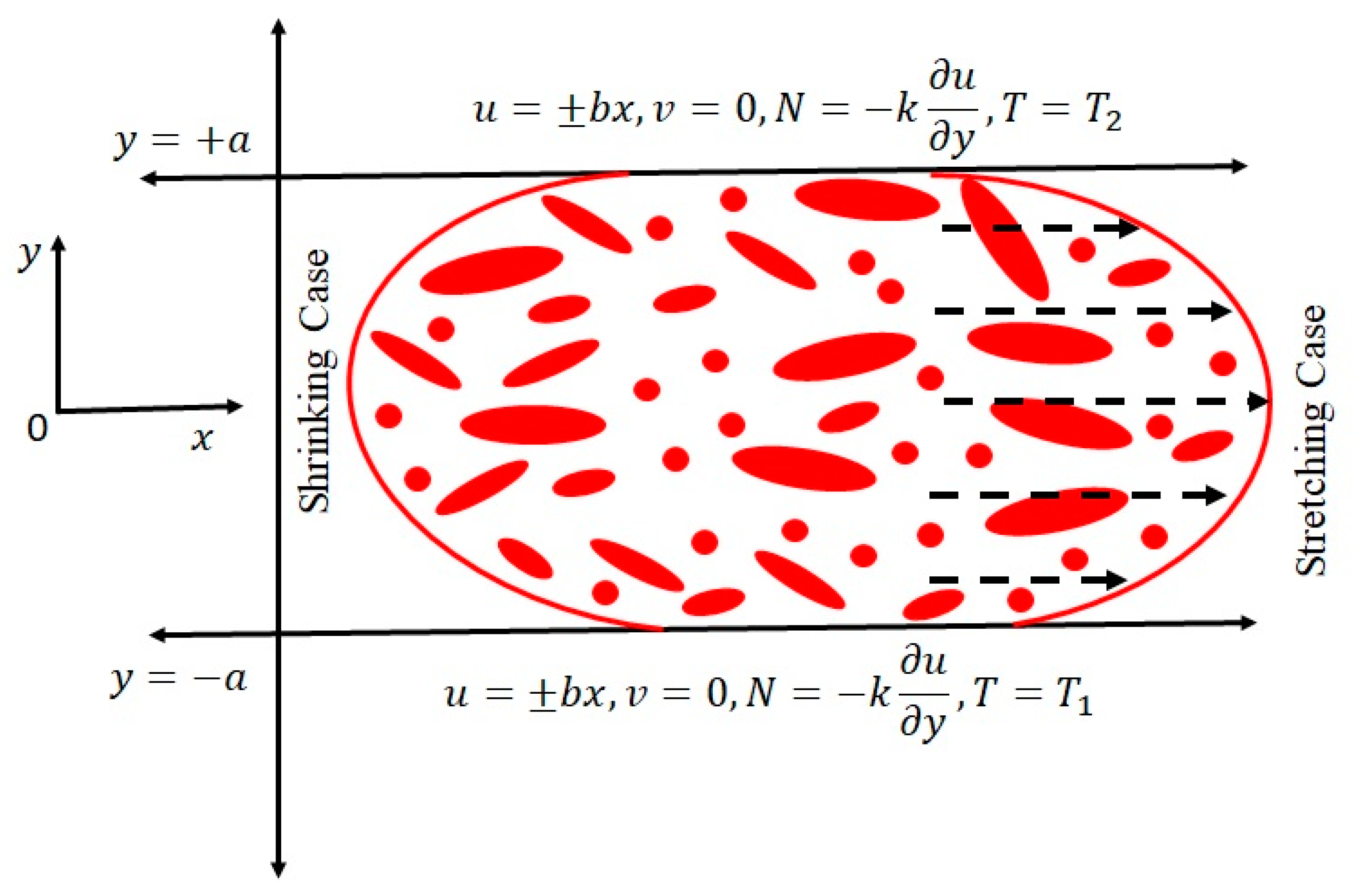
  • It proposes the single-phase nanofluid model of micropolar copper–blood nanoparticles in a channel with stretching and shrinking walls.
  • Thermal radiations are also present in the channel to make the problem more appealing for heat transfer.
  • To control the reversibility of the flow due to the stretching walls, we impose a transverse magnetic field.
  • This research also investigates sensitivity analysis using response surface methodology (RSM).

2. Proposed Model

Consider two-dimensional steady laminar incompressible micropolar nanofluid in a channel with stretching and shrinking walls in the presence of a magnetic field and thermal radiation. In this study, copper nanoparticles are the solid dispersed phase while blood is the fluid continuum phase. The lower and upper walls of the channel stretch and shrink in the direction of the fluid (x-axis) with some constant rate u = b x     b R . If b > 0 , then the case is known as stretching and b < 0 is for shrinking walls of the channel (see Figure 1).

2.1. Governing Equations

The general equations of micropolar fluids as given by Eringen [1] can be represented in component form V ¯ = ( u ( x , y ) , v ( x , y ) , 0 ) , ν ¯ = ( 0 , 0 , N ( x , y ) ) , where N = × V 0 as:
u x + v y = 0    
u u x + v u y = 1 ρ p x + μ + κ ρ 2 u + κ ρ N y σ f B ° 2 ρ n f u  
v x + v v y = 1 ρ p y + μ + κ ρ 2 v κ ρ N x
ρ n f j ¯ ( u N x + v N y ) = γ n f 2 N + κ ( v x u y ) 2 κ N
( u T x + v T y ) = k n f ( ρ C p ) n f ( 2 T x 2 + 2 T y 2 ) 1 ( ρ C p ) n f q r y  
Here, p is the pressure, N is the micro-rotational velocity, γ n f = j ( k 2 + μ n f ) is the spine gradient viscosity, and u and v are the axial and transverse velocities components, respectively.
The appropriate boundary conditions for the current investigation are:
u = ± b x ,   v = 0 ,   N = k u y ,   T = T 1   at   y = a
u = ± b x ,   v = 0 ,   N = k u y ,   T = T 2   at   y = + a
These physical quantities are described mathematically as:
ρ n f = ρ f ( 1 φ ) + φ ρ s  
μ n f = μ f ( 1 φ ) 2.5
( ρ C p ) n f = ( ρ C p ) f ( 1 φ ) + ( ρ C p ) s φ
k n f k f = k s + 2 k f 2 φ ( k f k s ) k s + 2 k f + φ ( k f k s )
Here, φ is the solid volume fraction, φ s is for the nanosolid-particles, and φ f is for the base fluid.
We apply a Rosseland approximation for radiation as:
q r = 4 σ * 3 k * T 4 y    
Here, the Stefan–Boltzmann constant is given by σ * = 5.6697 × 10 8   Wm 2 K 4 and the mean spectral absorption coefficient is denoted by k*. Further, blackbody emission power, eb in terms of the Stefan–Boltzmann constant and absolute temperature, is given by e b = σ * T 4 .
It is assumed that the temperature differences within the flow, such as the term T4, may be expressed as a linear function of temperature. We obtain the Taylor series expansion for T4 at a free stream temperature T.
T 4 = T 4 + 4 T 3 ( T T ) + 8 T 2 ( T T ) 2 +
After neglecting higher-order terms as:
T 4 = 4 T 4 T 3 T 4  
Using Equation (12) in (13), we obtain:
q r y = 16 σ * T 3 3 k * 2 T y 2
Equation (5) is now converted in the light of (14) as:
( ρ C p ) n f ( u T x + v T y ) = k n f ( 2 T x 2 + 2 T y 2 ) + 16 σ * T 3 3 k * 2 T y 2

2.2. Similarity Solution

Now we introduce the similarity transformation as:
η = y a , u = b x f ( η ) , v = a b f ( η ) , θ ( η ) = T T 2 T 1 T 2
Using Equation (16) in Equation (1), we see that Equation (1) is identically satisfied and eliminating the pressure term from (2) and (5), we obtain the required similarity coupled system of the ordinary differential equation as:
( 1 + κ Γ 2 ) f Γ 1 Γ 2 R ( f f f f ) κ Γ 2 g M 2 Γ 2 f = 0  
( 1 + κ 2 Γ 2 ) g + κ Γ 2 ( f 2 g ) + Γ 1 Γ 2 R ( f g f g ) = 0
1 Γ 3 P r ( Γ 4 + 4 3 R d ) θ + R f θ = 0
Subject to the boundary conditions:
f ( 1 ) = 0 ,   f ( 1 ) = ± 1 , g ( 1 ) = 0 , θ ( 1 ) = 1
f ( 1 ) = 0 ,   f ( 1 ) = ± 1 , g ( 1 ) = 0 , θ ( 1 ) = 0
Here, R = a 2 b ν f is the Reynolds number, M 2 = σ f B ° 2 a 2 μ f is the magnetic parameter, K = k ν f is the micropolar parameter, P r = ν f ( ρ C p ) f k f is the Prandtl number, and R d = σ * T 3 3 k * k f is the radiation parameter. Also,
Γ 1 = ( 1 φ ) + φ ρ s ρ f ,                 Γ 2 = 1 ( 1 φ ) 2.5 ,  
Γ 3 = ( 1 φ ) + ( ρ C p ) s ( ρ C p ) f φ ,   Γ 4 = k s + 2 k f 2 φ ( k f k s ) k s + 2 k f + φ ( k f k s )  

3. Results and Discussion

The numerical results have been handled in this section in the form of tables and graphs. Equations (17)–(19), subject to boundary conditions (20) and (21), are solved with the aid of a numerical scheme called Runge–Kutta 4th order and finite difference base scheme (bvp4c) [29]. Equations (17)–(19) are higher order ODEs, so we converted them into a system of first order ODEs, however three (03) initial conditions were missing ( d 2 f d η 2 | η = 0 , d 3 f d η 3 | η = 0 , d 2 g d η 2 | η = 0 , d θ d η | η = 0 ) . To find these missing initial conditions, we employed a shooting method. Once these missing conditions were found, then the solution computed and satisfied the boundary conditions (20) and (21). Thermophysical properties of blood and copper nanoparticles [27] are fetched from Table 1.
Figure 2, Figure 3, Figure 4, Figure 5, Figure 6, Figure 7, Figure 8, Figure 9, Figure 10, Figure 11 and Figure 12 provide information on the hydrokinetic effects on velocity, angular velocity, temperature, and concentration. The comparison of the two different approaches of the numerical results is presented graphically in Figure 2 and it is depicted that the results coincide with each other. Figure 3 depicts how the micropolar parameter affects the velocity profile f′( η ) for stretching and contracting the wall. The velocity profile, which is parabolic in character, is shown to decline as the micropolar parameter rises. However, we deduced from Figure 4 that the micro-rotation g( η ) profile gradually increases as the micropolar parameter K increases after decreasing from the bottom wall to the channel centre. The micro-rotation profile displays an entirely different pattern in the case of diminishing walls. On other hand, the temperature profile θ ( η ) rises while the walls are extending and falls when the walls are contracting. As can be observed from Figure 8, the velocity profile decreases as the solid volume percentage increases for stretching walls and rises for contracting walls. The impact of the stretching Reynolds number R on the velocity profile is explained in Figure 9. This graphic demonstrates how the velocity profile for the stretched walls reduces towards the channel borders and increases near the channel centre. However, it can be seen in Figure 10 that the micro-rotation profile rises from the lower wall to the channel’s centre, and then falls when the values of the Reynolds number for the stretched walls are raised. Figure 11 also illustrates the effect of the Reynolds number on the temperature profile. We can observe that the temperature profile changes for the bottom and upper halves of the channel when the Reynolds number values are increased. Figure 12 shows the effect of the radiation parameter on the temperature profile. The temperature profile of the tube drops from the lower wall to the middle and climbs from the centre to the top wall as the radiation parameter rises. The reverse result, however, can be seen in the case of the diminishing walls.

3.1. Application of Response Surface Methodology (RSM)

3.1.1. Optimization Process

RSM is one of many useful tools for describing a wide range of variables, together with limited resources, quantitative data, and the required test design (response surface methodology). The following steps were taken into account in this process:
  • To reach the suitable and believable requirements for the intended response, we planned and investigated the data values.
  • We outlined the most appropriate mathematical models for the response surface.
  • We described the mathematical models for the response surface that are most suited.
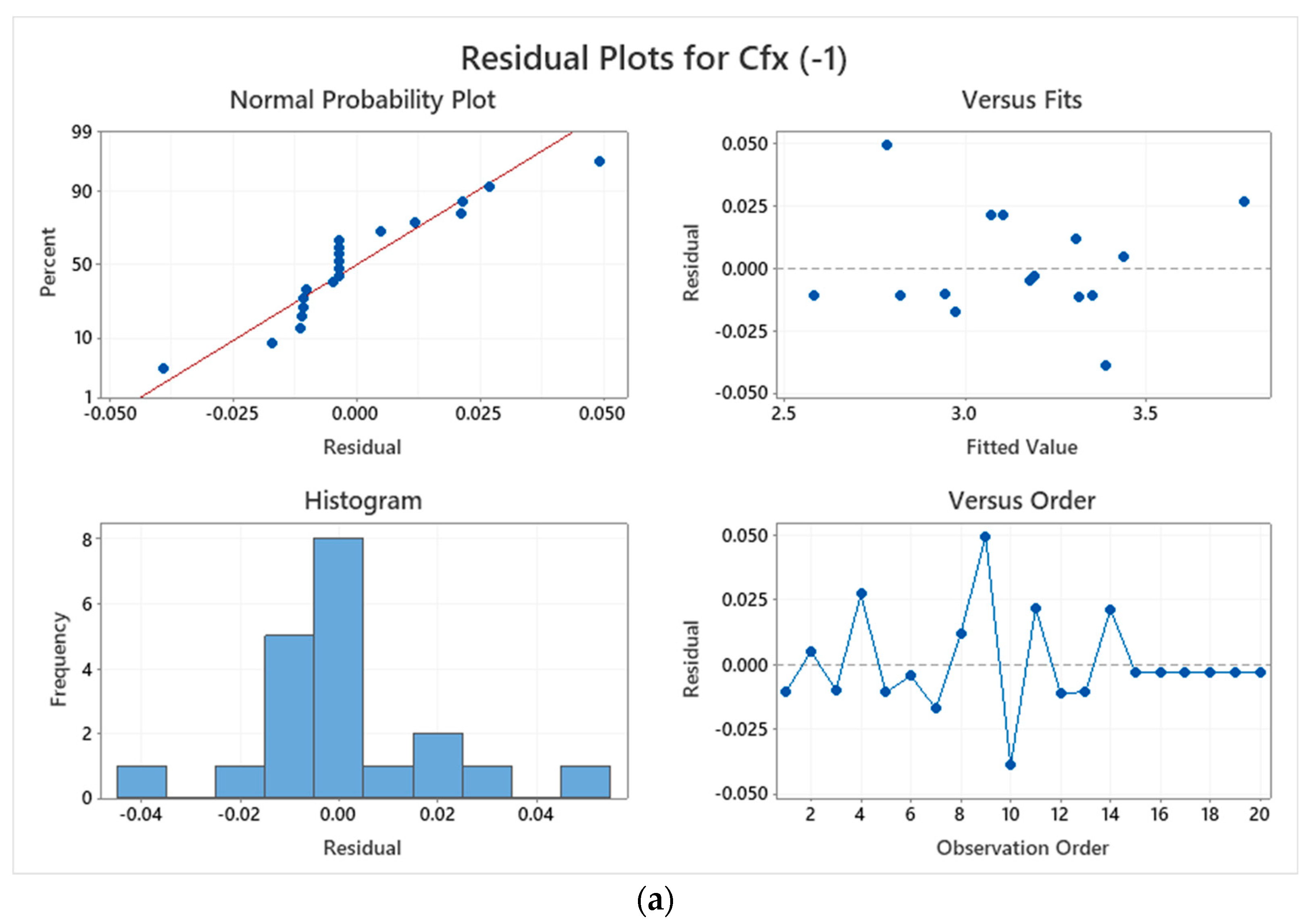
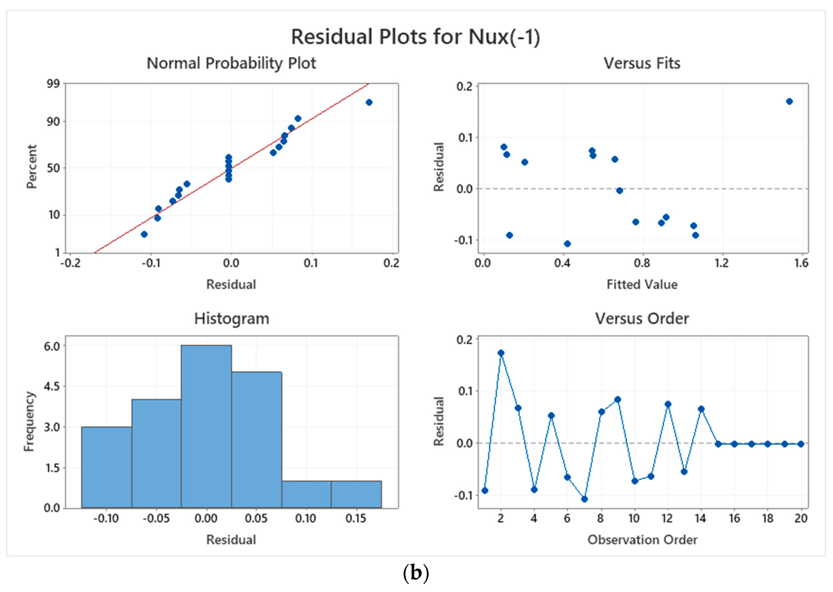
  • We used an analysis of the variance to examine the parametric direct and interaction impacts (ANOVA).

3.1.2. Optimization Analysis by RSM

The relation between the factor variables and the response variable (temperature gradient) was investigated using a face-centred central composite design. Table 2 and Table 3 indicates the three factors and their levels. The quadratic model is presented in Equation (22), where three linear, square, and interactive terms are involved.
Response = α 0 + α 1 A + α 2 B + α 3 C + α 11 A 2 + α 22 B 2 + α 33 C 2 + α 12 A B + α 13 A C + α 23 B C
Here (Equation (22)), α i and α i j represent the regression coefficients. The statistical analysis was performed for 20 runs, as prescribed by the defined conditions.
C f x ( 1 ) = 3.0015 + 0.08816 R + 0.1126 M 0.1056 K + 0.000686 R 2 + 0.0843 M 2 + 0.0479 K 2 0.00175 R M 0.02615 R K 0.0731 M K
N u x ( 1 ) = 0.758 + 0.1441 R 2.00 φ 0.288 R d + 0.00412 R 2 + 3.64 φ 2 + 0.0665 R d 2 0.2273 R φ 0.03759 R d . R + 0.614 φ R d
The values of skin friction coefficient and Nusselt number for coded values are given in Table 4. The ANOVA Table 5 and Table 6 provide a measure of accuracy for the approximate model. A parameter is important when the p-value is less than 0.05 (with 95 percent confidence). Since the p-value in the model is greater than 0.05, the linear, quadratic, and interaction terms may be omitted. Nonetheless, as seen in Table 5,6 the model proves to be superior since its coefficient of determination R2 is higher. The correct regression equation is now as follows:
C f x ( 1 ) = 3.0015 + 0.08816 R + 0.1126 M 0.1056 K + 0.0843 M 2 + 0.0479 K 2 0.02615 R K 0.0731 M K
N u x ( 1 ) = 0.758 + 0.1441 R 0.288 R d 0.03759 R d . R
Table 2 and Table 3 present the various levels of the parameters for C f x ( 1 ) and N u x ( 1 ) , respectively. However, Table 4 represents the values of the response function for 20 different points. In Table 5 and Table 6, the R2 for C f x ( 1 ) and N u x ( 1 ) (99.48% and 95.92% respectively), which was obtained by the testing methods and statistical analysis of the model, is presented. However, the R2-adj amounts for C f x ( 1 ) and N u x ( 1 ) (99.01% and 92.25%, respectively) are R2, but the model fits the data reasonably [30,31,32,33]. Moreover, the importance of the model for the response variables C f x ( 1 ) and N u x ( 1 ) is depicted from the F-value, which is equal to 211.26 and 26.11, respectively. According to Figure 13a,b, it is observed that the plots of normal probability are well-behaved and in good condition [33]. From these two figures, the residual histograms exhibit a skewed distribution. When the residual diagrams and fitted values were compared, the observed and fitted values showed a strong correlation.
Figure 14 and Figure 15 show the mean total skin friction coefficient and Nusselt number variations as effective parameters functions. The deviation of the skin friction coefficient in terms of M and R are shown in Figure 14a. The skin friction coefficient increases as M   and R are increased, with the highest value ( + 1 ) and lowest value ( 1 ) for M   and R , respectively. The variation in the response variable (skin friction) with respect to K and R are shown in Figure 14b. It is observed that reducing the values of K and increasing the value of R causes an increase in the skin friction coefficient. The highest value of skin friction is obtained in the level of (−1) and ( + 1 ) and its lowest value is observed in the level of ( + 1 ) and ( + 1 ) for K and R , respectively. The variance of the skin friction coefficient in terms of K and M is shown in Figure 14c. The skin friction is increased when the value of K is reduced and the value of M is increased. Furthermore, for K and M , the highest and lowest values of the skin friction coefficient can be found at the levels of (−1) and (+1), respectively. The variance of the total Nusselt number in terms of the solid volume fraction of a nanofluid and the Reynolds number R is shown in Figure 15a. The Nusselt number is increased when the solid volume fraction is lower and the Reynolds number is higher. Moreover, the Nusselt number gains its minimum value in ( + 1 ) and ( 1 ) and its maximum in ( 1 ) and ( + 1 ) for φ and R , respectively. Figure 15b shows that the Nusselt number increases by increasing the values of R and decreasing the values of R d . Nevertheless, the Nusselt number gains a maximum in level ( 1 ) and ( + 1 ) and a minimum in ( + 1 ) and ( 1 ) for R d and R , respectively. In the same vein, Figure 15c shows that the Nusselt number reaches its highest value in ( 1 ) and ( 1 ) and its lowest value in ( + 1 ) and ( + 1 ) for R d and the solid volume fraction.
The regression Equations (25) and (26) are used to calculate the sensitivity. The sensitivity functions are the partial derivatives of the response variables with respect to the factor variables, as shown below:
C f x A = 0.08816 0.02615 K
C f x B = 0.1126 + 0.1686 M 0.0731 K
C f x C = 0.1056 + 0.0958 K 0.02615 R 0.0731 M
N u x A = 0.1441 0.03759 R d
N u x B = 0
N u x C = 0.288 0.03759 R
The positive sensitivity value indicates that the objective function has improved as a result of the improved input parameters. Its negative value, on the other hand, denotes a decline in the objective function due to the increased input parameters. From Table 7, it is seen that the sensitivity of C f x to A and B is positive and negative for C. Similarly, from Table 8, the sensitivity of N u x to A is positive and negative for C.

4. Conclusions

In this investigation, we considered two-dimensional steady laminar incompressible micropolar nanofluid in a channel with stretching and shrinking walls in the presence of a magnetic field and thermal radiation. The copper nanoparticles are the solid dispersed phase, while blood is the fluid continuum phase. The lower and upper walls of the channel stretch and shrink in the direction of the fluid (x-axis). The governing similar ODEs were solved and verified by two different numerical schemes. After in-depth discussions of the model, the main findings are drawn as below:
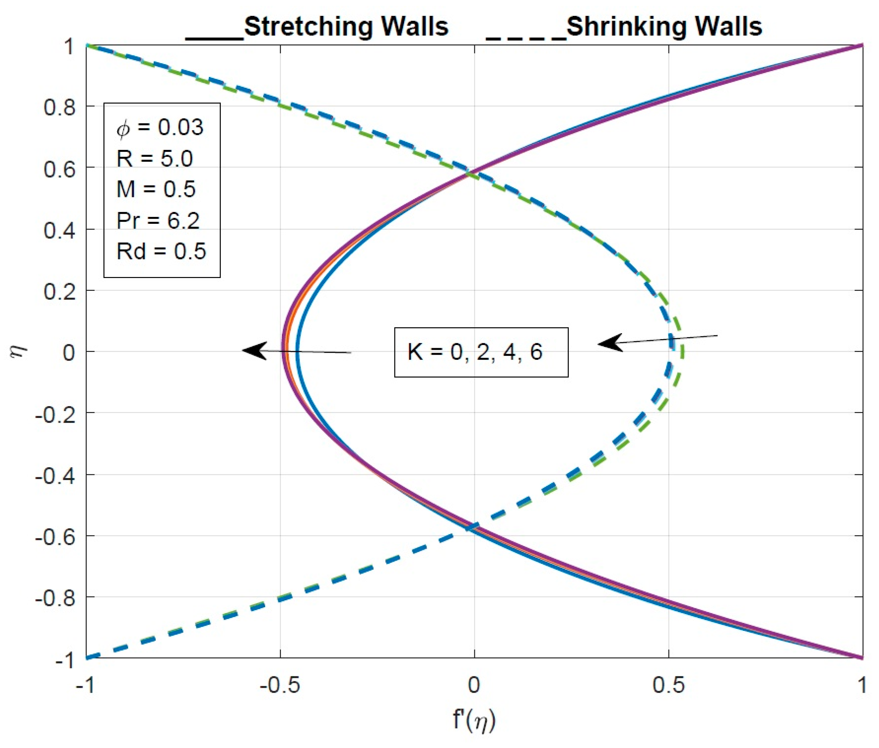
  • The velocity of the fluid particles decreases by increasing the values of the micropolar parameter.
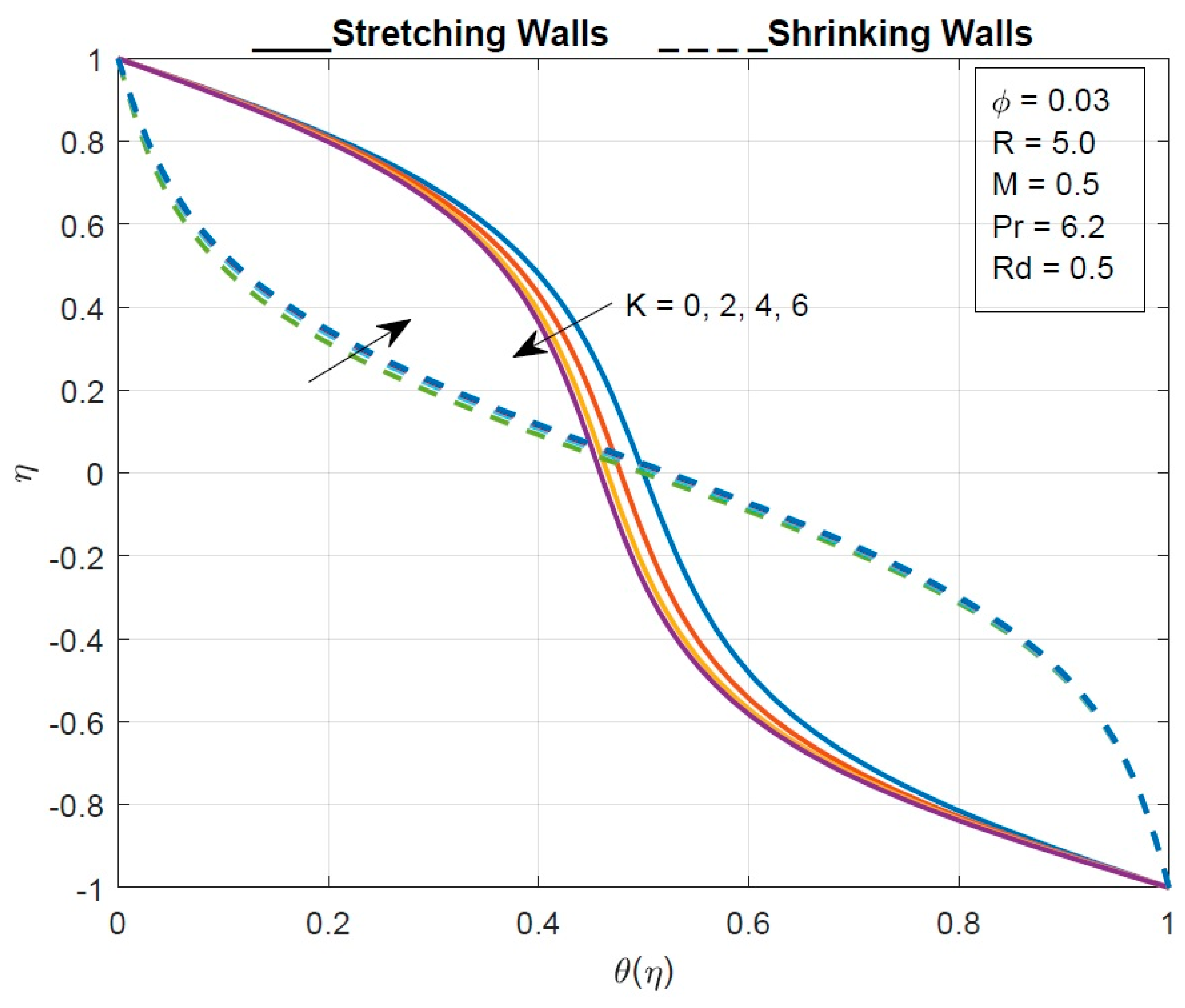
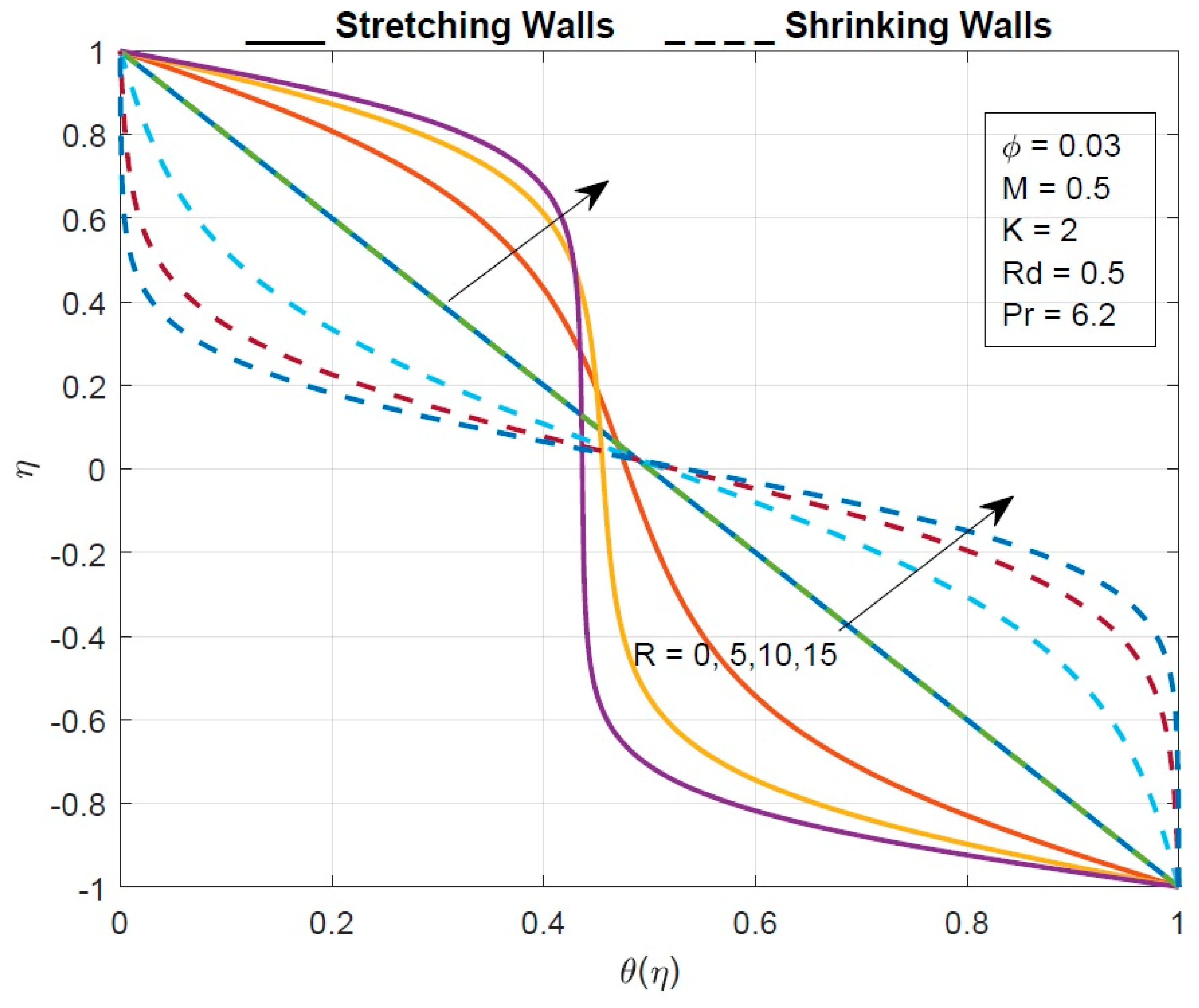
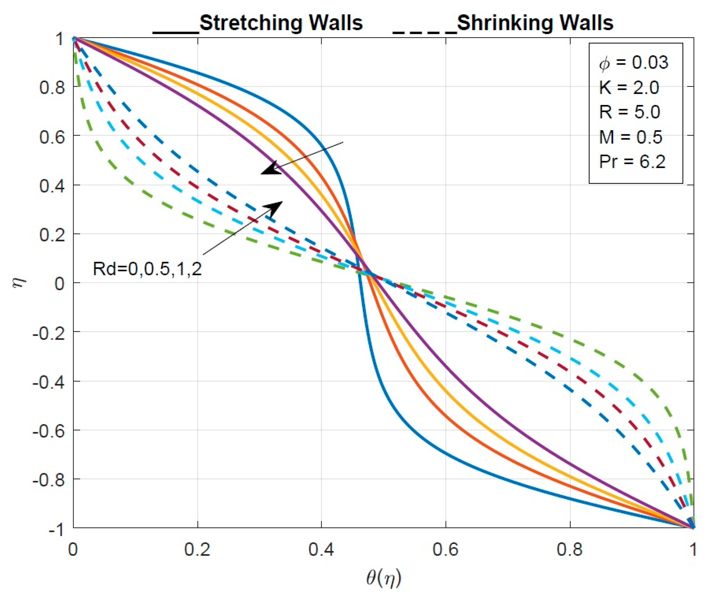
  • As the radiation parameter increases, the temperature profile decreases from the lower wall to the middle and increases from the centre to the upper wall of the tube.
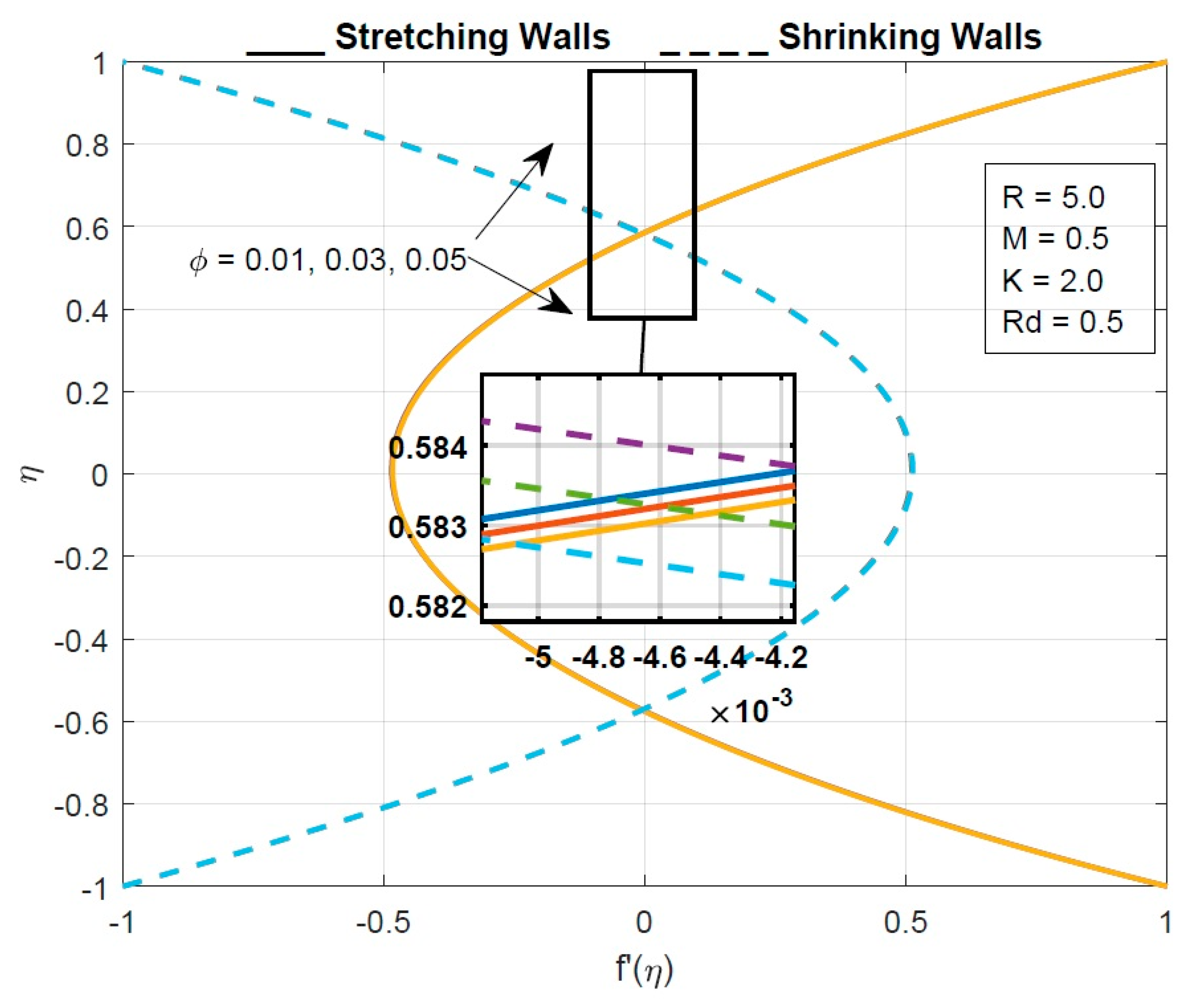
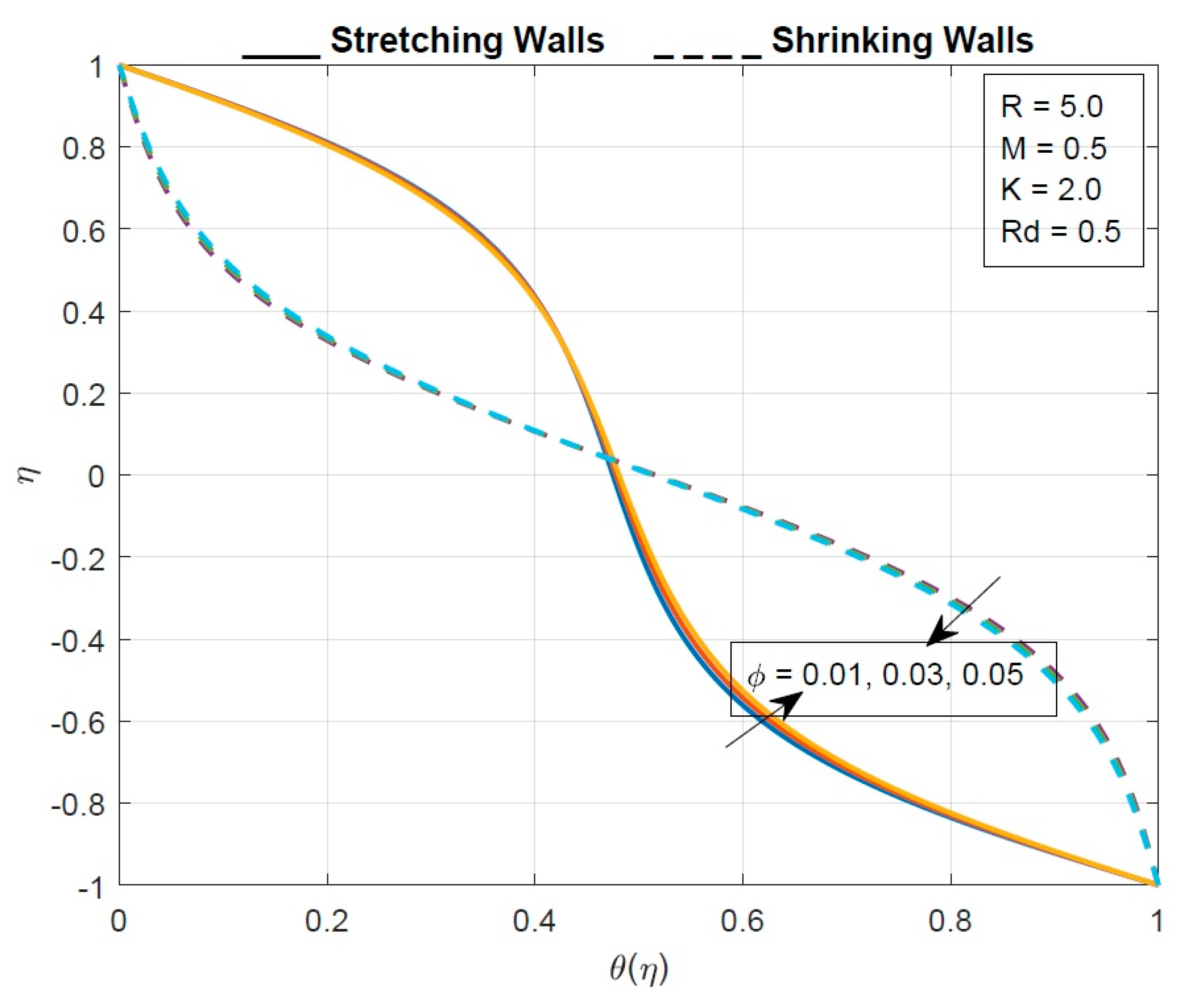
  • The velocity profile declines as a solid volume fraction ϕ enhances for the stretching walls and increases for the shrinking walls.
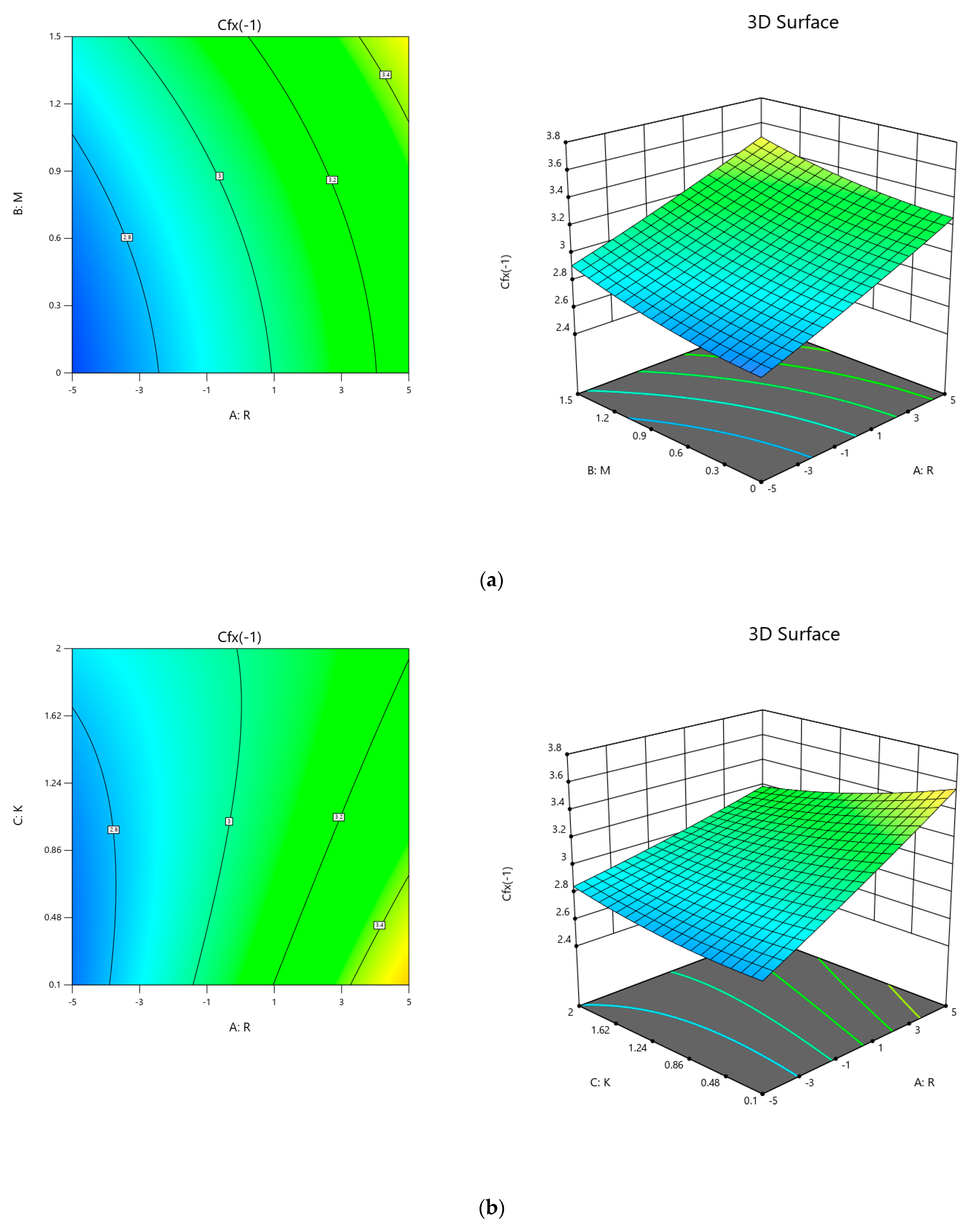
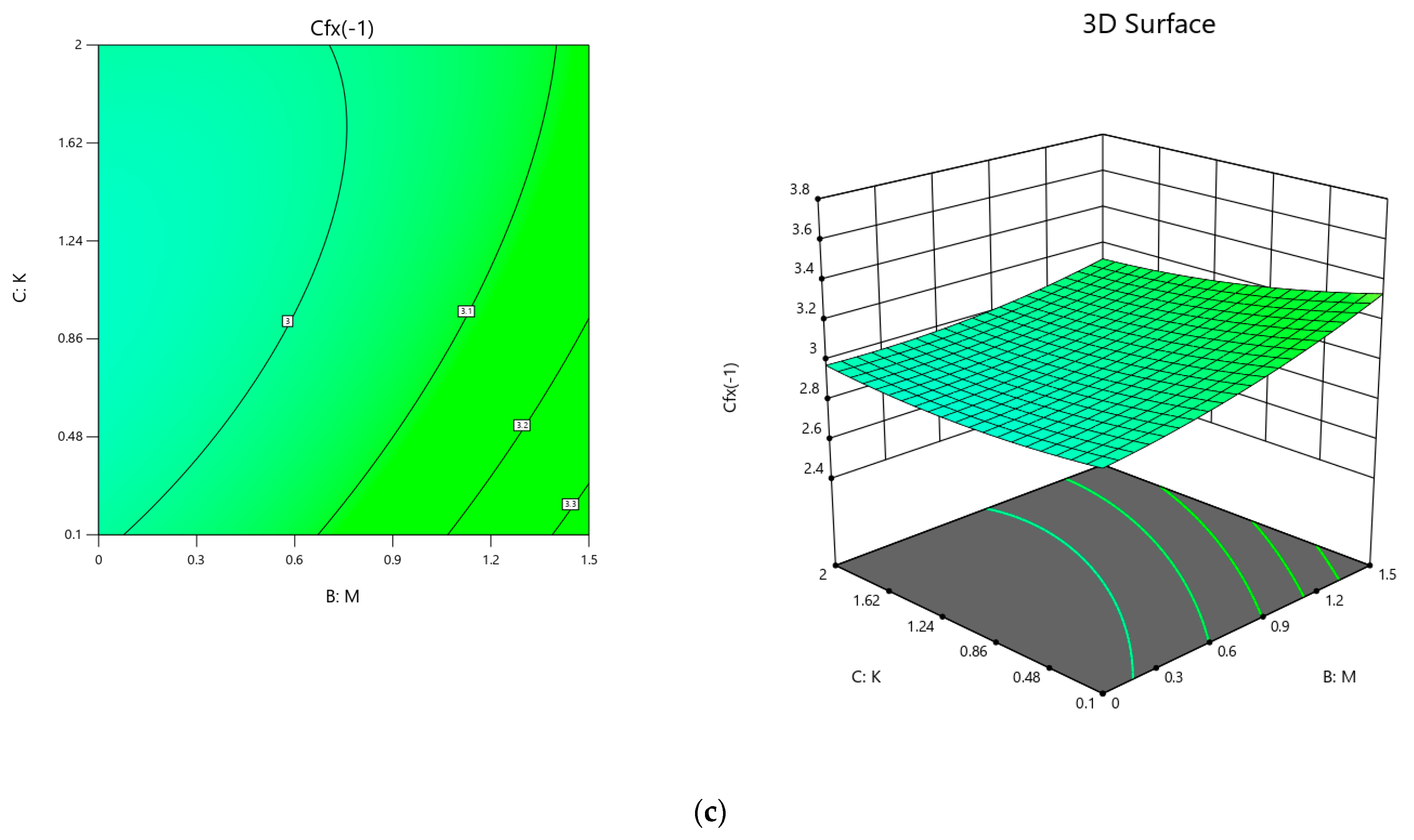
  • The skin friction coefficient increases as the magnetic and Reynolds number are increased.
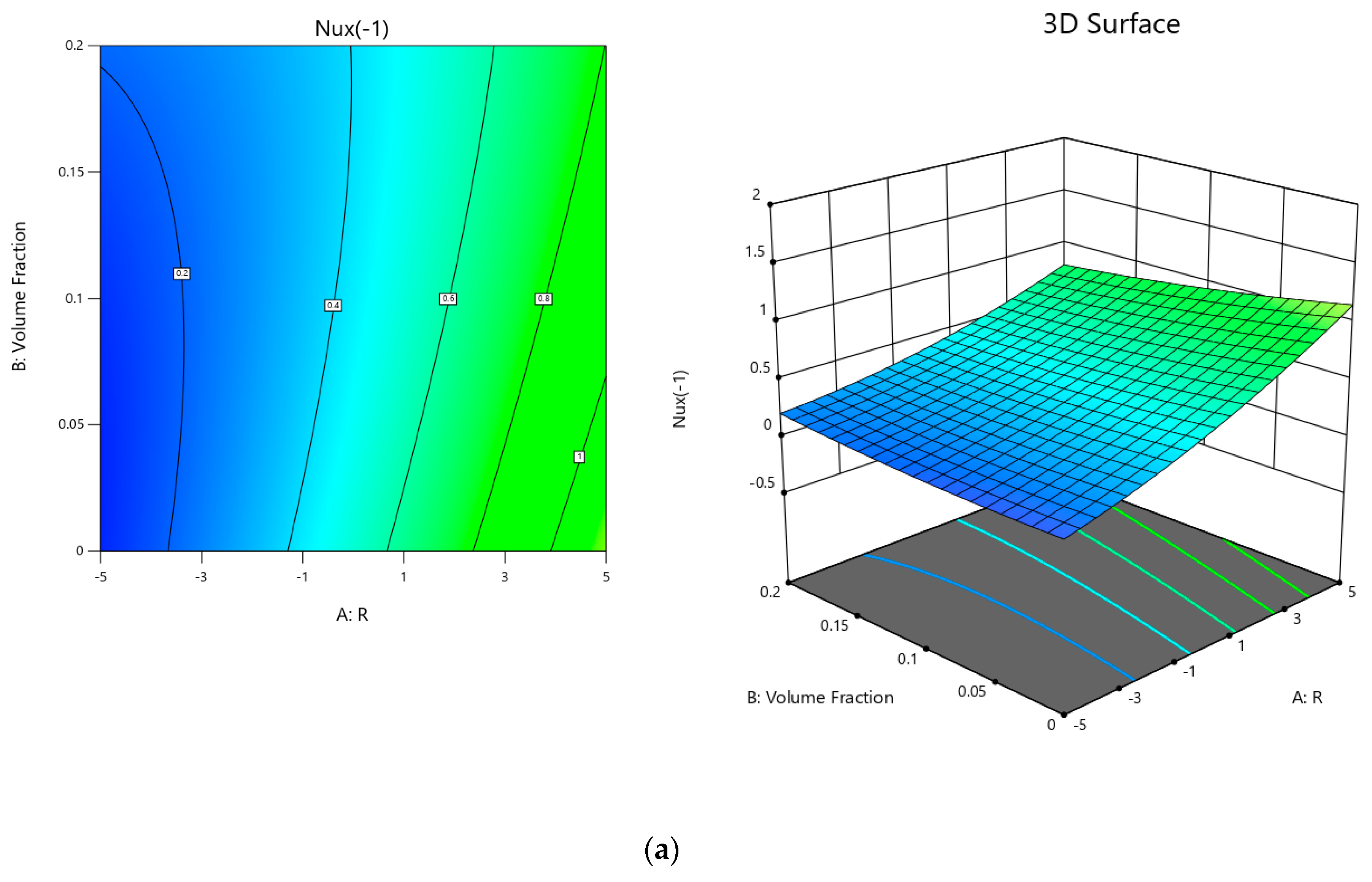
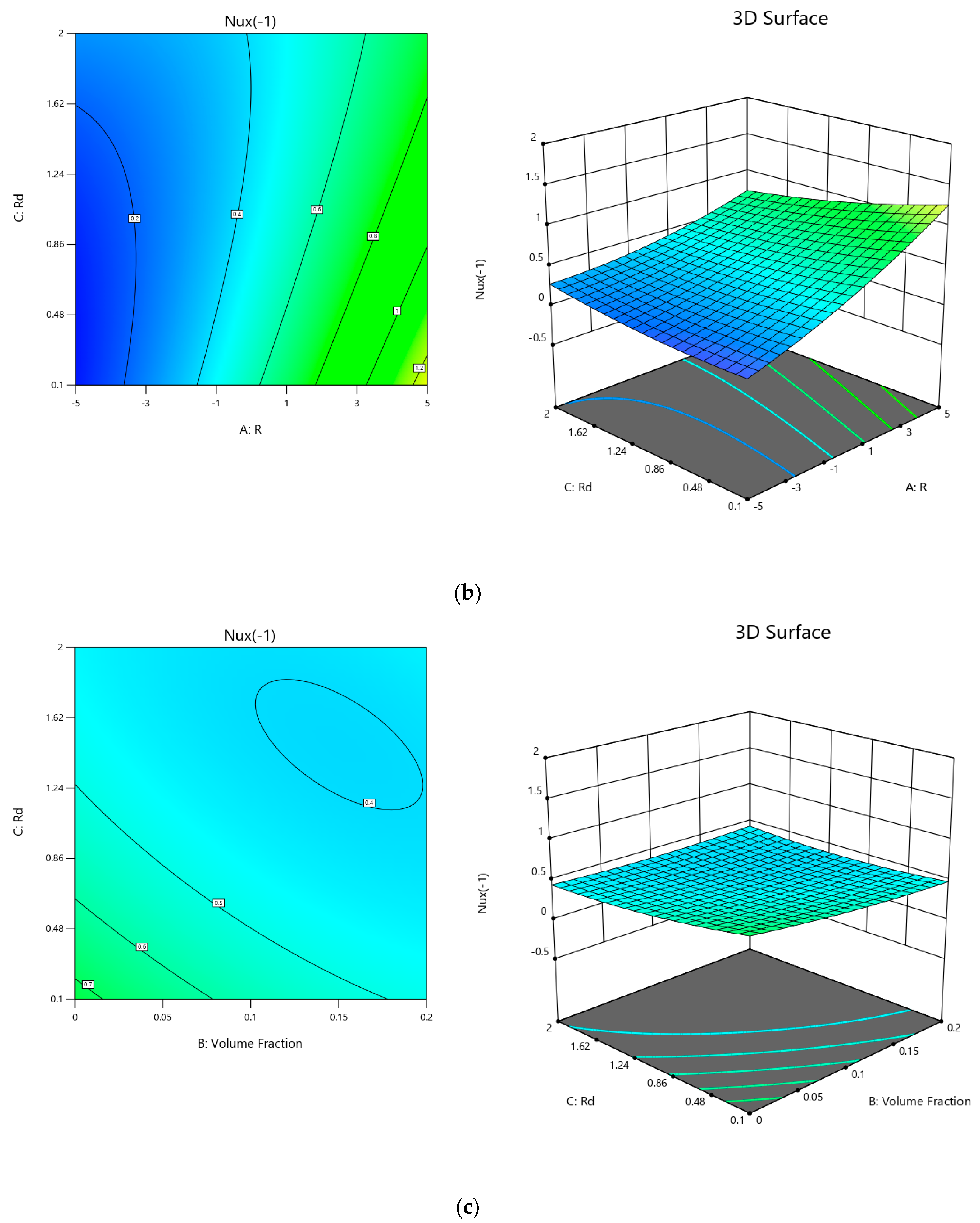
  • The Nusselt number is increased when the solid volume fraction is lower.
  • The sensitivity of C f x to the Reynolds number and magnetic parameter is positive and negative for the micropolar parameter.
  • N u x is optimized by taking higher values of the Reynolds number and lower values of the radiation parameter.

Author Contributions

Conceptualization, J.R. and T.M.; Methodology, R.A.A. and S.A.M.A.; Software, J.R., T.M., M.R.G. and A.M.H.; Validation, R.A.A. and M.R.G.; Formal analysis, S.A.M.A.; Investigation, M.R.G.; Resources, J.R. and A.M.H.; Data curation, T.M., S.A.M.A. and A.M.H.; Writing—original draft, J.R. and T.M.; Writing—review & editing, R.A.A. All authors have read and agreed to the published version of the manuscript.

Funding

Princess Nourah bint Abdulrahman University Researchers Supporting Project number (PNURSP2023R61), Princess Nourah bint Abdulrahman University, Riyadh, Saudi Arabia.

Data Availability Statement

Not applicable.

Acknowledgments

The authors express their gratitude to Princess Nourah bint Abdulrahman University Researchers Supporting Project number (PNURSP2023R61), Princess Nourah bint Abdulrahman University, Riyadh, Saudi Arabia.

Conflicts of Interest

The authors declare no conflict of interest.

References

  1. Eringen, A.C. Theory of micropolar fluids. J. Math. Mech. 1966, 16, 1–18. [Google Scholar] [CrossRef]
  2. Eringen, A.C. Theory of micropolar elasticity. In Microcontinuum Field Theories; Springer: New York, NY, USA, 1999; pp. 101–248. [Google Scholar]
  3. Mohammadein, A.A.; Gorla, R.S.R. Effects of transverse magnetic field on mixed convection in a micropolar fluid on a horizontal plate with vectored mass transfer. Acta Mech. 1996, 118, 1–12. [Google Scholar] [CrossRef]
  4. Peddieson, J. Boundary Layer Theory for a Micropolar Fluid. 1970. Available online: web (accessed on 1 January 2023).
  5. Gupta, P.S.; Gupta, A.S. Heat and mass transfer on a stretching sheet with suction or blowing. Can. J. Chem. Eng. 1977, 55, 744–746. [Google Scholar] [CrossRef]
  6. Chakrabarti, A.; Gupta, A.S. Hydromagnetic flow and heat transfer over a stretching sheet. Q. Appl. Math. 1979, 37, 73–78. [Google Scholar] [CrossRef]
  7. Incropera, F.P.; Bergman, T.L.; Lavine, A.S.; DeWitt, D.P. Fundamentals of Heat and Mass Transfer; Springer: New York, NY, USA, 2011. [Google Scholar]
  8. Cengel, Y.A.; Boles, M.A. Thermodynamics: An Engineering Approach, 8th ed.; McGraw-Hill: New York, NY, USA, 2015. [Google Scholar]
  9. Cengel, Y.A. Heat Transfer: A Practical Approach, 2nd ed.; McGraw-Hill: New York, NY, USA, 2002. [Google Scholar]
  10. Zhao, N.; Li, S.; Yang, J. A review on nanofluids: Data-driven modeling of thermalphysical properties and the application in automotive radiator. Renew Sustain. Energy Rev. 2016, 66, 596–616. [Google Scholar] [CrossRef]
  11. Krishna, V.M.; Kumar, M.S. Numerical analysis of forced convective heat transfer of nanofluids in microchannel for cooling electronic equipment. Mater. Today Proc. 2019, 17, 295–302. [Google Scholar] [CrossRef]
  12. Okonkwo, E.C.; Okwose, C.F.; Abid, M.; Ratlamwala, T.A.H. Second-law analysis and exergoeconomics optimization of a solar tower—Driven combined-cycle power plant using supercritical CO2. J. Energy Eng. ASCE 2018, 144, 04018021. [Google Scholar] [CrossRef]
  13. Okonkwo, E.C.; Abid, M.; Ratlamwala, T.A.H. Numerical analysis of heat transfer enhancement in a parabolic trough collector based on geometry modifications and working fluid usage. J. Sol. Energy Eng. 2018, 140, 0510091. [Google Scholar] [CrossRef]
  14. Meseguer, J.; Pérez-Grande, I.; Sanz-Andrés, A. Spacecraft Thermal Control, 1st ed.; Elsevier: London, UK, 2012. [Google Scholar]
  15. Sajid, M.U.; Ali, H.M. Thermal conductivity of hybrid nanofluids: A critical review. Int. J. Heat Mass Transf. 2018, 126, 211–234. [Google Scholar] [CrossRef]
  16. Das, S.K.; Choi, S.U.S.; Patel, H.E. Heat transfer in nanofluids—A review heat transfer in nanofluids. Heat Transf. Eng. 2007, 27, 37–41. [Google Scholar]
  17. Choi, S.U.; Eastman, J.A. Enhancing Thermal Conductivity of Fluids with Nanoparticles; No. ANL/MSD/CP-84938; CONF-951135-29; Argonne National Lab.: Lemont, IL, USA, 1995. [Google Scholar]
  18. Liu, L.H.; Métivier, R.; Wang, S.; Wang, H. Advanced nanohybrid materials: Surface modification and applications. J. Nanomater. 2012, 2012, 536405. [Google Scholar] [CrossRef]
  19. Rashid, I.; Haq, R.U.; Al-Mdallal, Q.M. Aligned magnetic field effects on water based metallic nanoparticles over a stretching sheet with PST and thermal radiation effects. Phys. E Low-Dimens. Syst. Nanostruct. 2017, 89, 33–42. [Google Scholar] [CrossRef]
  20. ul Haq, R.; Aman, S. Water functionalized CuO nanoparticles filled in a partially heated trapezoidal cavity with inner heated obstacle: FEM approach. Int. J. Heat Mass Transf. 2019, 128, 401–417. [Google Scholar] [CrossRef]
  21. Hayat, T.; Imtiaz, M.; Alsaedi, A. Melting heat transfer in the MHD flow of Cu–water nanofluid with viscous dissipation and Joule heating. Adv. Powder Technol. 2016, 27, 1301–1308. [Google Scholar] [CrossRef]
  22. Sandeep, N.; Sharma, R.P.; Ferdows, M. Enhanced heat transfer in unsteady magnetohydrodynamic nanofluid flow embedded with aluminum alloy nanoparticles. J. Mol. Liq. 2017, 234, 437–443. [Google Scholar] [CrossRef]
  23. Shah, F.; Khan, M.I.; Hayat, T.; Khan, M.I.; Alsaedi, A.; Khan, W.A. Theoretical and mathematical analysis of entropy generation in fluid flow subject to aluminum and ethylene glycol nanoparticles. Comput. Methods Programs Biomed. 2019, 182, 105057. [Google Scholar] [CrossRef] [PubMed]
  24. Misra, J.C.; Shit, G.C.; Rath, H.J. Flow and heat transfer of a MHD viscoelastic fluid in a channel with stretching walls: Some applications to haemodynamics. Comput. Fluids 2008, 37, 1–11. [Google Scholar] [CrossRef]
  25. Ashraf, M.; Jameel, N.; Ali, K. MHD non-Newtonian micropolar fluid flow and heat transfer in channel with stretching walls. Appl. Math. Mech. 2013, 34, 1263–1276. [Google Scholar] [CrossRef]
  26. Raza, J.; Rohni, A.M.; Omar, Z. MHD flow and heat transfer of Cu–water nanofluid in a semi porous channel with stretching walls. Int. J. Heat Mass Transf. 2016, 103, 336–340. [Google Scholar] [CrossRef]
  27. Reza, J.; Mebarek-Oudina, F.; Makinde, O.D. MHD slip flow of Cu-Kerosene nanofluid in a channel with stretching walls using 3-stage Lobatto IIIA formula. In Defect and Diffusion Forum; Trans Tech Publications Ltd.: Wollerau, Switzerland, 2018; Volume 387, pp. 51–62. [Google Scholar]
  28. Raza, J.; Rohni, A.M.; Omar, Z. Numerical investigation of copper-water (Cu-water) nanofluid with different shapes of nanoparticles in a channel with stretching wall: Slip effects. Math. Comput. Appl. 2016, 21, 43. [Google Scholar] [CrossRef]
  29. Lund, L.A.; Omar, Z.; Raza, J.; Khan, I. Magnetohydrodynamic flow of Cu–Fe 3 O 4/H 2 O hybrid nanofluid with effect of viscous dissipation: Dual similarity solutions. J. Therm. Anal. Calorim. 2021, 143, 915–927. [Google Scholar] [CrossRef]
  30. Chan, S.Q.; Aman, F.; Mansur, S. Sensitivity analysis on thermal conductivity characteristics of a water-based bionanofluid flow past a wedge surface. Math. Probl. Eng. 2018, 2018, 9410167. [Google Scholar] [CrossRef]
  31. Vahedi, S.M.; Pordanjani, A.H.; Raisi, A.; Chamkha, A.J. Sensitivity analysis and optimization of MHD forced convection of a Cu-water nanofluid flow past a wedge. Eur. Phys. J. Plus 2019, 134, 124. [Google Scholar] [CrossRef]
  32. Khan, N.S.; Kumam, P.; Thounthong, P. Second law analysis with effects of Arrhenius activation energy and binary chemical reaction on nanofluid flow. Sci. Rep. 2020, 10, 19792. [Google Scholar] [CrossRef]
  33. Thriveni, K.; Mahanthesh, B. Significance of variable fluid properties on hybrid nanoliquid flow in a micro-annulus with quadratic convection and quadratic thermal radiation: Response surface methodology. Int. Commun. Heat Mass Transf. 2021, 124, 105264. [Google Scholar] [CrossRef]
Figure 1. Physical sketch of the problem.
Mathematics 11 00939 g001
Figure 2. Code verification.
Mathematics 11 00939 g002
Figure 3. The effect of the micropolar parameter on the velocity profile.
Mathematics 11 00939 g003
Figure 4. The effect of the micropolar parameter on the micro-rotation.
Mathematics 11 00939 g004
Figure 5. The effect of the micropolar parameter on the temperature profile.
Mathematics 11 00939 g005
Figure 6. The effect of the solid volume fraction on the velocity profile.
Mathematics 11 00939 g006
Figure 7. The effect of the solid volume fraction on the micro-rotation profile.
Mathematics 11 00939 g007
Figure 8. The effect of the solid volume fraction on the temperature profile.
Mathematics 11 00939 g008
Figure 9. The effect of the Reynolds number on the velocity profile.
Mathematics 11 00939 g009
Figure 10. The effect of the Reynolds number on the micro-rotation profile.
Mathematics 11 00939 g010
Figure 11. The effect of the Reynolds number on the temperature profile.
Mathematics 11 00939 g011
Figure 12. The effect of the radiation parameter on the temperature profile.
Mathematics 11 00939 g012
Figure 13. Residual plot for (a) C f x (b).
Mathematics 11 00939 g013aMathematics 11 00939 g013b
Figure 14. Three-dimensional surfaces and contour plots for all continuous parameters of M, R, and K on Cfx.
Mathematics 11 00939 g014aMathematics 11 00939 g014b
Figure 15. Three-dimensional surfaces and contour plots for all continuous parameters of R, Phi, and Rd on Nux.
Mathematics 11 00939 g015aMathematics 11 00939 g015b
Table 1. Thermophysical properties of the blood and copper nanoparticles (see [27]).
PropertiesBloodCopper
Density   ( Kg m 3 ) 11508933
Thermal   conductivity   ( W mK ) 0.53401
Specific   Heat   ( JKg 1 K 1 ) 3617385
Table 2. Parameters with their levels for C f x ( 1 ) .
ParametersSymbolsLevel
−101
R A−525
M B011.5
K C0.112
Table 3. Parameters with their levels N u x ( 1 ) .
ParametersSymbolsLevel
−101
R A−525
φ B00.050.2
R d C0.112
Table 4. Experimental design and responses.
RunsCoded Values
ABC Response   C f x ( 1 ) Response   N u x ( 1 )
1−1−1−12.5699776540.039218876
21−1−13.44120491.706219612
3−11−12.9313692250.182650354
411−13.7977084280.975161305
5−1−112.8086659940.256515544
61−113.1735242210.828662877
7−1112.9546898810.315102036
81113.3159636270.717271607
9−1002.8325517270.185583893
101003.3470065340.981815599
110−103.0920575920.701100814
120103.3028405440.617231054
1300−13.3404859460.860674809
140013.1243840460.614658362
150003.1873626370.679561304
160003.1873626370.679561304
170003.1873626370.679561304
180003.1873626370.679561304
190003.1873626370.679561304
200003.1873626370.679561304
Table 5. ANOVA for C f x ( 1 ) .
SourceDFAdjusted Sum of SquareAdjusted Mean SquareF-Valuep-ValueRemarks
Model91.274990.141666211.260.000Significant
Linear31.051110.350369522.480.000Significant
R10.877030.8770271307.850.000Significant
M10.146950.146950219.140.000Significant
K10.032010.03201047.730.000Significant
Square30.034350.01145117.080.000Significant
R.R10.000550.0005460.810.388Not Significant
M.M10.004740.0047387.070.024Significant
K.K10.005090.0050937.590.020Significant
2-Way Interaction30.152760.05091975.930.000Significant
R.M10.000360.0003620.540.480Not Significant
R.K10.127390.127394189.970.000Significant
M.K10.022200.02220433.110.000Significant
Error100.006710.000671
Lack-of-Fit50.006710.001341**
Pure Error50.000000.000000
Total191.28170
R 2 = 99.48% Adjusted   R 2 = 99.01%
Table 6. ANOVA for N u x ( 1 ) .
SourceDFAdj SSAdj MSF-Valuep-ValueRemarks
Model92.394520.2660626.110.000Significant
Linear31.761270.5870957.620.000Significant
R11.659701.65970162.900.000Significant
Phi10.039050.039053.830.079Not Significant
Rd10.067700.067706.640.028Significant
Square30.099990.033333.270.067Not Significant
R.R10.019700.019701.930.194Not Significant
Phi.Phi10.001910.001910.190.674Not Significant
Rd.Rd10.009820.009820.960.349Not Significant
2-Way Interaction30.412880.1376313.510.001Significant
R.Phi10.112030.1120311.000.008Not Significant
R.Rd10.262920.2629225.810.000Significant
Phi.Rd10.028550.028552.800.125Not Significant
Error100.101880.01019
Lack-of-Fit50.101880.02038**
Pure Error50.000000.00000
Total192.49640
R 2 = 95.92% Adjusted   R 2 = 92.25%
Table 7. Sensitivity analysis of the response C f x .
ABCSensitivity to ASensitivity to BSensitivity to C
0−1−10.114310.0171−0.1283
0−100.08816−0.056−0.0325
0−110.06201−0.12910.0633
00−10.114310.1857−0.2014
0000.088160.1126−0.1056
0010.062010.0395−0.0098
01−10.114310.3543−0.2745
0100.088160.2812−0.1787
0110.062010.2081−0.0829
Table 8. Sensitivity analysis of the response N u x .
ABCSensitivity to ASensitivity to BSensitivity to C
−10−10.181690−0.25041
−1000.14410−0.25041
−1010.106510−0.25041
00−10.181690−0.288
0000.14410−0.288
0010.106510−0.288
10−10.181690−0.32559
1000.14410−0.32559
1010.106510−0.32559
Disclaimer/Publisher’s Note: The statements, opinions and data contained in all publications are solely those of the individual author(s) and contributor(s) and not of MDPI and/or the editor(s). MDPI and/or the editor(s) disclaim responsibility for any injury to people or property resulting from any ideas, methods, instructions or products referred to in the content.

