1. Introduction
Recently, elements of digital transformation have become increasingly visible and in demand in various areas of human activity, including healthcare.
The digital transformation of healthcare is a continuous process aimed at completely restructuring the mechanisms of work of industry authorities, medical organizations and their interaction with patients. The introduction of advanced digital technologies ensures high standards of medical care and the transition to the “4P medicine” model (preventive, personalized, participatory, predictive medicine) [
1].
The introduction of digital technologies in healthcare should ensure a decrease in the level of morbidity and mortality of the population and an increase in life expectancy, including active life expectancy. The use of health monitoring technologies should allow not only for the detection of pathologies at an early stage, but also to prevent the development of diseases.
The development of technologies for analyzing large volumes of medical data, including the use of artificial intelligence, will make it possible to obtain new knowledge in the field of medicine and biology, as well as to develop new methods for diagnosing and treating diseases.
The transformation of healthcare under the influence of digital technologies is taking place everywhere, including such areas as:
Transition from standardized clinical protocols to a personalized approach to patient care due to the accumulation of a large amount of medical data, as well as the widespread use of individual biomonitoring devices;
Disease prevention through early diagnosis and regular health monitoring using wearable devices;
Patient focus and active involvement of the patient in the treatment process.
At the same time, the demand for applied and computational mathematics’ tools for digital environments becomes obvious in the case of solving problems of disease prevention through early diagnosis, including cancer [
2,
3,
4,
5].
Oncological diseases (ODs) are among the most dangerous ones because they can lead to serious consequences for patients, especially in the case of late diagnosis. Such consequences include significant pain and a difficult psychological state. The treatment of oncological diseases is usually lengthy and involves significant financial costs both for the patients and their families and for the state.
An OD is an immune disease that first causes the division and growth of abnormal cells in a single organ of the patient, and then can quickly spread to the entire body.
Obviously, early diagnosis of an OD should allow the oncologist to choose an adequate and effective treatment regimen for the patient in a timely manner. However, the task of early diagnosis of an OD is very difficult: unfortunately, the typical symptoms of ODs appear only in the later stages when the disease is difficult to treat, so the treatment may ultimately turn out to be unsuccessful.
One of the approaches to the early diagnosis of an OD is based on the analysis of test results, in particular, gene tests (GTs) [
4,
6] and protein tests (PTs) [
4,
7,
8]. GTs reveal hereditary information, they are static, difficult to interpret, and are usually used to detect congenital genetic diseases [
4]. Such tests do not detect diseases that occur when there are problems with the immune system and metabolism. In addition, GTs are expensive. PTs, unlike GTs, are dynamic and they allow (if carried out in a timely manner) for identifying the occurrence of an OD and track its development [
4]. Additionally, PTs are non-invasive, painless for patients and affordable.
The diagnosis of ODs based on blood protein markers has been increasingly used in the last few years [
4,
9,
10]. Presumably, PT-based diagnostic technologies will allow for predicting the risks of developing oncological diseases 1–3 years in advance, which will make it possible to take advanced preventive measures against the emergence and development of an OD.
There are many different types of protein markers in the blood, and the values of the markers are different for different types of ODs [
4]. It is obvious that the use of only one type of marker or some limited group of markers reduces the accuracy of diagnosing ODs, even if this marker (or group of markers) is recognized as the standard for diagnosis. One of the reasons leading to the refusal to use the full range of PTs results is the limited ability of specialists to interpret the data. It is easier to operate with information about the values of 1–2 protein markers than with data on the values of several dozen of the same markers (especially if specialists use a unified table with a priori given limits of the norm and abnormality, followed by a decision based on their knowledge and intuition). It can be reasonably assumed that the use of the full range of PTs results should improve the accuracy of diagnosing various ODs.
It is obvious that the involvement of modern technologies of data mining and machine learning will make it possible to reveal the knowledge about the relationship between the values of blood protein markers in various types of ODs hidden in the PT results.
Currently, data mining and machine learning technologies are actively used to solve various problems of medical diagnostics, including solving the problems of diagnosing ODs [
10,
11,
12,
13,
14,
15,
16,
17,
18,
19]. In this case, classifiers are developed based on appropriate datasets. The k-Nearest Neighbors (kNN) algorithm [
10], SVM (Support Vector Machine) algorithm [
11], Decision Tree (DT) algorithm [
12], Random Forest (RF) algorithm [
15], their hybrids and deep learning algorithms [
17,
18,
19] are most broadly used in creating such classifiers.
The main problem in the development of tools for solving problems of medical diagnostics is the imbalance of classes in the dataset [
10,
20]: usually, normal data patterns characterizing cases when the disease is absent constitute the majority class, while data patterns of interest and characterizing cases when certain diseases are present constitute the corresponding minority classes. In this case, for example, instead of developing a binary classifier based on an imbalanced dataset, it becomes necessary to develop a multiclass classifier based on an imbalanced dataset, which is a non-trivial task, since it is necessary to teach the classifier to separate data from different classes that are imbalanced. Obviously, a binary classifier can be obtained even in the case of class imbalance (for example, in a ratio of 10:1), and the accuracy of it will be 90% (which is not bad in the case of balanced classes), but such accuracy should be considered bad if the classifier made errors on all objects from the minority class.
Data scientists have proposed various approaches to solve the problem of class imbalance:
Approaches using various class balancing algorithms that implement oversampling technologies (for example, SMOTE algorithm (Synthetic Minority Oversampling Technique) [
21,
22,
23], ADASYN algorithm (Adaptive Synthetic Sampling Approach) [
24]), undersampling technologies (for example, Tomek Links algorithm) [
23,
25] and their combinations;
Approaches that apply algorithms that account for the sensitivity to the cost of wrong decisions (cost-sensitive algorithms) [
10];
Approaches that implement the transfer of data into a space of a new dimension (with a decrease [
26,
27,
28,
29,
30,
31,
32] or increase [
11,
33,
34] in dimension), in which data classes will be separated from each other better than in the original space;
Approaches that implement the so-called one-class classification [
34,
35,
36,
37].
It should be noted that the transition to the space of a new dimension can be implemented in various ways, for example, using:
Dimension reduction algorithms (linear [
26,
27] and non-linear [
28,
29,
30,
31,
32]) that allow one to move to a space of lower dimension;
Kernel functions (as it is done in the SVM-algorithm, which allows the transition to a space of higher dimension) [
11,
33,
34,
36];
Algorithms for engineering (generation) of new features for data patterns, which make it possible to move to a space of higher dimension [
38].
All of these approaches have their advantages and disadvantages, and there is no universal methodology for choosing the approach that is appropriate to apply to the dataset used in the development of the data classifier.
In each case, it is necessary to perform a comprehensive analysis in order to:
Avoid loss of information during undersampling or reducing the dimension of the data space;
Exclude the introduction of false or redundant information during oversampling or increasing the dimension of the data space.
One of the obvious tools that can be used in assessing the quality of the developed classifier is detailed analysis of various classification quality metrics on the test sample, including metrics that allow for accounting for the specifics of the dataset, namely, its imbalance (for example, it is appropriate to use metrics such as Balanced accuracy and ). In addition, it is advisable to use cross-validation, including k-fold cross-validation, which makes it possible to empirically evaluate the generalizing ability of the developed classifier.
A large number of papers have been devoted to the problem of analyzing medical datasets containing information about blood protein markers and making decisions on the diagnosis of ODs. In particular, in the pilot study [
4], the task was to identify and surgically localize eight types of resectable ODs (ovary, liver, stomach, pancreas, esophagus, colorectum, lung and breast) based on a multi-analysis blood test using the CancerSEEK test [
4,
5] based on a machine learning algorithm called the logistic regression algorithm. The dataset used in the study is publicly available and located in the Catalog of Somatic Mutations in Cancer (COSMIC) repository [
39] as NIHMS982921-supplement-Tables_S1_to_S11.xlsx, and it is constantly updated with new data. The original dataset is available in the Supplementary Material for the paper as aar3247_cohen_sm_tables-s1-s11.xlsx [
4]. The eight types of ODs considered in the dataset were chosen by the authors because they are the most common among the population of Western countries, and also because blood-based tests are not used in clinical practice for their early detection.
The authors of the pilot study [
4] proposed to assess the levels of circulating proteins and mutations in cell-free DNA and use the obtained data in the LC (logistic classifier)-based CancerSEEK test. The study used 1005 data patterns received from patients with non-metastatic clinically identified ovarian, liver, stomach, pancreas, esophagus, colon, lung or breast ODs. The CancerSEEK test was based on screening results, such as the levels of protein biomarkers and ctDNA (Circulating tumor DNA). The authors proposed to take into account each person’s gender, the levels of eight proteins and the presence of mutations in 1933 different genomic positions, each of which can mutate in several ways.
It was assumed that the presence of a mutation in the analyzed gene or an increase in the level of any of the eight proteins makes it possible to classify the patient’s pattern as positive, i.e., a pattern with an identified OD. The authors used logarithmic ratios to evaluate the mutations and included them in a logistic regression algorithm (and, accordingly, in the LC), which took into account both the mutation data and the protein biomarker levels to evaluate the results of the CancerSEEK test. At the same time, the average values of sensitivity and specificity were determined from the results of 10 iterations using 10-fold cross validation.
The results of the experiments in [
4] showed that the average value of the
Sensitivity metric for eight types of ODs is about 70%, the highest value of the sensitivity metric is achieved for the ovary class (98%), slightly less for the liver class (close to 98%), and the lowest value of the sensitivity metric is achieved for the breast class (33%). In general, the values of the
Sensitivity metric ranged from 69 to 98% in the detection of five types of ODs (esophagus, pancreas, stomach, liver and ovaries, listed in ascending order of values of the
Sensitivity metric). The value of the metric specificity was above 99%: only 7 of the 812 patterns without known cancers scored positive. At the same time, as the authors write, there is no certainty that several false-positive patterns of patients identified in the normal class do not actually have an undiscovered OD. However, the classification of these patterns as false positives can be considered the most conservative approach to the classification and interpretation of medical data.
The average sensitivity of the CancerSEEK test was 73% for stage II cancer, which is the most common, 78% for stage III cancer, and less than 43% for stage I cancer. The highest and the lowest sensitivity for stage I cancer (the earliest stage) was recorded for liver cancer (100%) and esophageal cancer (20%), respectively.
A liquid biopsy involves deriving mutant DNA templates from dying cancer cells. Later on, these templates serve as specific neoplasia markers. The authors of the pilot study [
4] found that the mutation in blood plasma was identical to the mutation found in the primary tumor of the same person in 90% of analyzed cases diagnosed with ODs. This correspondence between the plasma and primary tumor was evident for all eight types of cancer and ranged from 100% for ovarian and pancreatic cancer to 82% for gastric cancer. One disadvantage of liquid biopsies is the inability to determine the type of cancer in patients with positive tests, leading to clinical problems for follow-up.
The authors of the pilot study [
4] point out that the vast majority of information about the localization of ODs was obtained from protein markers, since mutations in the driver gene are usually not tissue-specific. They propose the LC that implements the CancerSEEK test for the presence of eight common types of ODs. During the development of the LC, the authors used a training set that combined information about the levels of the gene and protein biomarkers. In doing so, they were able to increase the sensitivity of the CancerSEEK test without a significant decrease in specificity. The authors note that the effectiveness of combining completely different agents with different mechanisms of action is widely recognized in therapy, but not usually used in diagnostics. They also believe that other cancer biomarkers, such as metabolites, mRNA transcripts, microRNAs or methylated DNA sequences, can be similarly combined to increase the sensitivity and localization of a cancer focus.
The followers of the authors of the pilot study continued to offer their own versions of classifiers that implement the diagnosis of ODs based on datasets on values of blood protein markers without taking gene markers into account.
For example, in [
10], the authors proposed to use a cost-sensitive kNN algorithm based on a three-class imbalanced dataset containing patterns characterized by 39 blood protein markers and belonging to one of three classes: normal, ovary and liver. In order to include the hidden information in the data analysis and improve the quality of the classification, the authors used two entropy metrics: approximate entropy AE and sample entropy SE. At the time that the study was conducted, the analyzed dataset contained 897 patterns from three classes in the ratio Normal:Ovary:Liver = 799:54:44. The overall accuracy of the classifier was equal to 0.952, and the values of such metrics as
Precision,
Recall,
and
AUC were equal to 0.807, 0.833, 0.819 and 0.920, respectively.
It should be noted that the authors of this work abandoned the attempt to develop a classifier for nine classes (eight classes corresponding to patterns of various types of ODs, and one class corresponding to patterns for which no ODs were diagnosed) due to poor separability of the classes.
The goal of this study is to develop the high-precision data classifiers on ODs using modern tools for data mining and machine learning technologies. It is supposed to develop kNN [
10,
34] and SVM [
11,
33,
34,
36] classifiers using oversampling algorithms SMOTE [
21], Borderline SMOTE-1 [
22], Borderline SMOTE-2 [
22] and ADASYN [
24], which allow for restoring the balance of classes in the original and extended datasets, formed on the base of the original dataset with the application of various techniques for extracting new features. In particular, it is planned to consider:
The UMAP (Uniform Manifold Approximation and Projection) algorithm [
29,
30,
31,
32], which implements non-linear data dimensionality reduction by embedding data into a space of lower dimensionality to generate new features based on pattern features;
Formulas for calculating entropies [
40,
41,
42,
43,
44,
45], Hjorth parameters [
46,
47] and fractal dimensions [
48,
49,
50,
51,
52] in order to generate new features based on the pattern features.
This study presents the first attempt to generate datasets that involve different tools with the subsequent selection of the best of them to form new features by extracting information hidden in the features of the original dataset. The generation of new features was carried out using the UMAP algorithm, as well as various formulas for calculating entropies, Hjorth parameters and fractal dimensions. Various combinations of new features were selected based on correlation and the perceived ability to distinguish between patterns of different classes were added to the features of the original dataset or combined to form a new dataset. As a result, it becomes possible to work simultaneously with different datasets that describe the subject area. This approach to the generation of datasets is used for the first time in the field of medical diagnostics, including the field of diagnostics of oncological diseases based on blood protein markers. Subsequently, these datasets are balanced using oversampling algorithms and are used in the development of classifiers based on the kNN and SVM algorithms with subsequent selection of the best classifiers based on classification quality metrics.
The rest of the paper is organized as follows.
Section 2 briefly describes the aspects of developing the kNN and SVM classifiers. It also discusses the applied quality metrics of multiclass classification, as well as the problem of class imbalance in datasets. In addition, this section provides a summary of the principles of operation of the UMAP algorithm, as well as background information on the investigated nonlinear data extraction tools that are difficult to obtain from traditional statistics, in particular, on entropy characteristics and fractal dimensions.
Section 3 presents a description of the novel approach to the formation of the datasets used in the development of the classifiers.
Section 4 is devoted to the analysis of the original dataset based on the UMAP algorithm with data visualization, aspects of the generation of new features based on entropy characteristics and fractal dimensions of the data patterns, choosing the best of them. It also discusses all of the steps of the creation of new datasets used for the development of the kNN and SVM classifiers and the results of the development of such classifiers, accompanied by tables and figures.
Section 5 presents a discussion of the proposed results. Finally,
Section 6 contains conclusions and goals regarding future work.
2. Materials and Methods
2.1. Aspects of Development of Classifiers
The development of classifiers can be performed using various machine learning algorithms, for example, kNN [
10,
34,
53,
54,
55,
56], SVM [
10,
33,
34,
36,
57,
58], LR (Logistic Regression) [
4,
59], DT [
12,
13,
14], RF [
15,
60,
61] and neural networks [
17,
18,
19], as well as cascade algorithms and ensembles based on them. We can use the default values of the classifier parameters, or fine-tune them using population optimization algorithms [
62,
63]. The quality of classification using such classifiers will depend both on the quality of datasets on the basis of which the classifiers are developed, and on the specifics of the mathematical apparatus embedded in the algorithms corresponding to the classifiers. Currently, there is no universal machine learning algorithm that could ensure that a classifier developed on its basis will provide high quality of classification for any arbitrary training dataset. The same can be said about cascade classifiers and ensembles of classifiers. Obviously, it is desirable to minimize the time for developing a classifier that provides high-quality data classification.
Two machine learning algorithms (kNN and SVM) are considered in this study, although all the ideas formulated below can be used in the development of classifiers based on any machine learning algorithm because they affect only the stage of preparation of datasets used in the development of classifiers.
The choice of the kNN algorithm is due to the simplicity of its implementation and, as a result, low time costs for the development of the kNN classifier.
The choice of the SVM algorithm is due to the availability of tools for working with various kernel functions that provide a transition to a higher-dimensional space, and the possibility of generating classification rules in an explicit form by identifying the so-called support vectors located along the class boundary. However, the time spent on the development of the SVM classifier becomes significantly larger compared to the time spent on the development of the kNN classifier.
It is precisely because of the large time costs for the development of the RF classifier that the proposed study does not consider the RF algorithm, although when it is used, it is usually possible to obtain classifiers that provide a very high quality of data classification.
Let
be a dataset used in the development of classifiers, where
;
;
;
is the number of patterns in the dataset;
is the number of classes;
is the set of signs of patterns; and
is the set of pattern class labels [
34].
Let classifiers be trained on patterns and testing be carried out on patterns. The quality of the classifiers is assessed using the k-fold cross-validation procedure.
2.1.1. kNN Classifier Development
The number of nearest neighbors k for the pattern and the method of voting for k nearest neighbors on the question of the class membership of the pattern are specified during the development of the binary kNN classifier. The values of the parameters should provide the minimum classification error.
The membership class
of a pattern
is determined by the membership class of most of the patterns from among the
k nearest neighbors of the pattern
. Various metrics, such as Euclidean, cosine, Manhattan, etc. can be used to calculate the distance between patterns in the kNN algorithm. Usually, the distance is calculated using the Euclidean distance metric as [
34,
53,
54]:
where
is the number of features of patterns
(
) and
;
is the
-th coordinate of
-th pattern
; and
is the
-th coordinate of pattern
.
Various voting methods can be used to determine the membership class of a pattern during the development of the kNN classifier, for example, simple unweighted voting and weighted voting [
34,
53,
54].
Simple unweighted voting works in such a way that the distance from the pattern
to each of the
k nearest neighbors
(
) does not matter: each of the
k nearest neighbors
(
) of the pattern votes for its assignment to its class, and all
k nearest neighbors
(
) have equal rights in class definition for pattern
. The pattern
will be assigned to the class that receives the most votes:
Weighted voting works in such a way that the distance from the pattern
to each of the
k nearest neighbors
(
) is taken into account: the smaller the distance
, the more significant the contribution to the estimation of the pattern
belonging to a certain class is made by the vote of the nearest neighbor
(
). The total contribution of the votes of the nearest neighbors
(
) for the pattern
belonging to the class with the label
can be calculated as:
where
, if
and
, if
.
The class that received the highest value according to Formula (3) is assigned to the pattern .
The problem of finding the optimal values of the parameters of the kNN classifier, for example, the number of neighbors and the voting method, can be solved using grid search algorithms or evolutionary optimization algorithms, such as the genetic algorithm, differential evolution algorithm, PSO algorithm, bee algorithm, ant colony algorithm, fish school algorithm, etc.
2.1.2. SVM Classifier Development
The SVM algorithm implements binary classification [
34,
57,
58]. In the case of multiclass classification, i.e., for
, strategies such as OvO (One-vs-One) or OvR (One-vs-Rest) are used, which allow for the use of binary classification solutions to form solutions for multiclass classification [
64].
The One-vs-One strategy breaks the multiclass classification into one binary classification problem for each pair of classes. The One-vs-Rest strategy breaks the multiclass classification into one binary classification problem for each class.
In the case of binary classification, the basic SVM algorithm operates on patterns with class labels .
The development of the SVM classifier can be performed using kernel functions such as linear, polynomial, radial basis and sigmoid kernel functions. Particularly, the linear kernel function has the form , and the radial basic kernel function, which is used in this study, has the form , where is the scalar product for and and () is the kernel function parameter.
The value of the regularization parameter
(
) [
57], the type of the kernel function
and the values of the parameters of the kernel function (for example, the value of parameter
for the radial basis kernel function) are determined during the development of the binary SVM classifier. The values of the parameters should provide the minimum classification error.
The development of the binary SVM classifier involves solving the problem of construction of a hyperplane separating the classes. According to the Kuhn–Tucker theorem, this problem can be reduced to a quadratic programming problem containing only dual variables
(
) [
34,
57,
58]:
The support vectors are determined as a result of the training of the binary SVM classifier. These are feature vectors of learning patterns
, for which the values of the corresponding dual variables
are not equal to zero (
) [
57]. The support vectors carry all the information about class separation since they are located near the hyperplane separating them.
The classification decision rule that assigns a membership class to a pattern with the label “−1” or “+1” is defined as [
34,
57,
58]:
where
;
.
The problem of finding the optimal values of the SVM classifier parameters, for example, the regularization parameter (), the type of the kernel function and the values of the parameters of the kernel function, can be solved using grid search algorithms or evolutionary optimization algorithms.
2.2. Quality Metrics of Multiclass Classification
The assessment of the quality of a multiclass classification can be performed using metrics such as
Accuracy,
,
MacroRecall and
[
65].
The
accuracy metric for multiclass classification can be calculated as:
where
is the total number of true positive elements in the multiclass classification problem;
is the total number of true negative elements in the multiclass classification problem;
is the total number of false positive elements in the multiclass classification problem; and
is the total number of false negative elements in the multiclass classification problem.
The
metric for multiclass classification can be calculated as:
where
is the class label index;
is the number of true positive elements for the
-th class label;
is the number of false positive elements for the
-th class label; and
is the total number of classes in the multiclass classification problem.
The
metric for multiclass classification can be calculated as:
where
is the class label index;
is the number of true positive elements for the
-th class label;
is the number of false negative elements for the
-th class label; and
is the total number of classes in the multiclass classification problem.
The
metric for multiclass classification can be calculated as:
Such metrics as (7)–(9) are useful and effective when developing classifiers using imbalanced datasets.
The is used as a maximized classification quality metric. Based on and , this metric makes it possible to simultaneously account for information on precision and recall of the solutions generated by the classifiers.
2.3. Solving the Class Imbalance Problem
In most machine learning algorithms, it is assumed that the goal of learning is to maximize the proportion of correct decisions in relation to all decisions made, and both the population and training dataset obey the same distribution. In this case, the datasets used to develop classifiers should be class-balanced, and the cost of a classification error for all patterns should be the same.
However, in many practical problems, one has to work with datasets that are poorly balanced. Learning on imbalanced datasets (imbalance problem) [
66,
67] can lead to a significant decrease in the quality of the classification solutions obtained using classifiers developed on their basis, since such datasets do not provide the required data distribution characteristics used in training.
For example, in the case of binary classification, the imbalance of the dataset is that more of the patterns in the dataset belong to one class, which is commonly called “majority”, and a much smaller set of patterns belongs to another class, which is commonly called “minority”.
The cost of misclassifying minority class patterns is often many times more expensive than misclassifying majority class patterns, because minority class objects in real datasets represent rare but most important instances.
For example, in the context of developing classifiers based on a dataset for ODs, the class of normal patterns is the majority, while the classes describing eight types of ODs are minor. Obviously, the correct classification of patterns of minority classes both for the problem under consideration and in general is of significant interest.
There are various approaches to solving the problem of class imbalance based on the application of:
Class balancing algorithms that implement oversampling, undersampling and their combinations [
21,
22,
23,
24,
25];
Algorithms accounting for the sensitivity to the cost of wrong decisions [
10];
Algorithms for transferring data into a space of a new dimension (with a decrease or increase in dimension) in order to improve the separability of data [
11,
26,
27,
28,
29,
30,
31,
32,
33,
34];
One-class classification algorithms [
34,
35,
36,
37].
In this study, the imbalance problem is proposed to be solved using such oversampling algorithms as SMOTE [
21], Borderline-SMOTE-1 [
22], Borderline-SMOTE-2 [
22] and ADASYN [
24], followed by choosing the best of them in the sense of providing a higher quality of data classification.
The use of oversampling algorithms is due to the fear of losing critical data patterns in the case of using undersampling algorithms in the context of the problem of developing classifiers for diagnosing oncological diseases.
The SMOTE (synthetic minority oversampling technique) algorithm [
21] randomly selects a minority class pattern named
a and randomly chooses a pattern named
b from the
k nearest neighbors of pattern
a. The synthetic pattern will be located randomly in the line segment between the original pattern
a and its neighbor
b. The same process will be repeated until the desired number of synthetic patterns is reached.
The Borderline-SMOTE-1 algorithm [
22] considers only the minority class patterns that have a number of minority class neighbors in the range [
g/2,
g], where
g is defined by the researcher. These are the borderline patterns and they can be easily misclassified, i.e., they are “in danger”. After detecting such original patterns, a basic SMOTE algorithm is applied to create synthetic patterns.
The Borderline-SMOTE-2 algorithm [
22] is similar to the Borderline-SMOTE-1 algorithm, but it also considers the neighbors of the majority class.
The ADASYN algorithm [
24] is similar to the SMOTE algorithm, since it generates synthetic patterns in the line segments between two minority class original patterns. It uses a weighted distribution for different minority class patterns that takes into account their level of difficulty: the minority class patterns that have fewer minority class neighbors are harder to learn than those which have more neighbors of the same class. The ADASYN algorithm generates more synthetic patterns for the minority class original patterns that are harder to learn and generates less for the minority class original patterns that are easier to learn.
2.4. UMAP Algorithm
The UMAP algorithm performs nonlinear dimensionality reduction preserving both local and global structures of high dimensional data in the best possible way [
29,
32] compared to other similar algorithms, for example, compared to the t-SNE algorithm [
28].
The UMAP algorithm builds a fuzzy weighted undirected graph in the first step and optimizes loss function in the second step [
29].
The UMAP algorithm works with a dataset , which contains objects (patterns). Every object is represented by -dimensional vector: . The UMAP algorithm embeds objects from the -dimensional space into the -dimensional space ().
In the first step, the UMAP algorithm searches for the
nearest neighbors
for every object
, where
;
, as described in [
68]. Then it computes the scalar distance value
between
and
using a distance metric. In the case of working with a Euclidean distance metric, the scalar
can be calculated as (1), where pattern
is replaced by
and
is replaced by
. As a result, for each object
, the UMAP algorithm determines a set
, which contains the distances between
and each of its
nearest neighbors.
After that, a fuzzy simplicial set, represented as a vector
, is constructed for each object. First, the UMAP algorithm searches for
, such that
for every
. After that, a binary search is implemented in order to find
satisfying the following condition:
Then the
j-th component of vector
is represented by a fuzzy value, which shows how similar
i-th and
j-th objects from the
set are. Therefore, if the two objects,
and
, are not neighbors, then the
j-th component
of vector
is set to 0. If the two objects,
and
, are neighbors, then the
j-th component
of vector
is computed as:
It is necessary to say that .
The UMAP algorithm defines a vector for each object . This vector encodes fuzzy similarities between the i-th object and every j-th object belonging to the original high dimensional dataset .
As a result, the UMAP algorithm builds a weighted adjacency matrix , where each i-th row is represented by fuzzy vector ().
The weighted adjacency matrix represents a fuzzy weighted oriented graph, which codes pairwise similarities of objects from . Matrix is not symmetric.
In the second step, the asymmetric matrix
is symmetrized using probabilistic t-conorm:
where
and
are the numbers of rows and columns in the
matrix, respectively (
).
Thus, the transformed matrix will already be symmetric.
The initial low dimensional representations of objects from the set
described by
-dimensional vectors in the
are calculated using spectral embedding [
32] (
). As a result, the matrix
is obtained.
Then the UMAP algorithm starts the optimization process using the weighted fuzzy cross-entropy with reduced repulsion as the loss function [
69]:
where
is the symmetric adjacency matrix containing fuzzy values encoding pairwise similarities of high dimensional objects from the dataset
;
is the representation of
objects in the low dimensional space
;
is a scalar value defining the fuzzy similarity of
i-th and
j-th high dimensional objects from the original dataset
; and
is a scalar value defining the fuzzy similarity of
i-th and
j-th objects in low dimensional space
.
The UMAP algorithm determines the pairwise similarity
of the
i-th and
j-th objects represented by the
i-th and
j-th rows of the
matrix in the low dimensional space
as:
where
is the scalar value between the
i-th and
j-th objects, described by vectors
and
corresponding to the rows in the matrix
.
The scalar value
can be computed using a Euclidean distance metric (1), assuming vectors
and
in (1) are replaced by vectors
and
, respectively, and
is replaced with
;
and
are the coefficients that are chosen by non-linear least squares fitting of (14) against the curve:
where
is the distance value between the
i-th and
j-th objects
and
represented by rows in the matrix
; and
is the parameter of the UMAP algorithm (
), which affects the density of the clusters formed during the loss function (13) optimization process in the low dimensional space
.
The UMAP algorithm performs the optimization of the loss function (13) using the stochastic gradient descent (SGD) algorithm [
29]. The locations of objects, which are described by rows of the matrix
, are specified during each iteration of the SGD algorithm in order to minimize the loss function (13). Other functions given, particularly in [
34], can also be used as a loss function.
2.5. Entropies, Hjorth Parameters and Fractal Dimensions
A number of works have shown that the use of nonlinear approaches can help extract some information from the data that is difficult to obtain from traditional statistics. In particular, entropy analysis and fractal analysis are non-linear approaches and provide researchers with new opportunities to extract and explore the knowledge hidden in the data. Entropy and fractal dimension are two diametrically opposed but complementary concepts.
Entropy is a measure of chaos. The value of entropy gives an idea of how far the studied object (pattern) is from an ordered, structured state and how close it is to a completely chaotic, structureless, homogeneous form.
Fractal dimension is a metric for characterizing a fractal pattern (which is often a highly organized structure) by quantifying its complexity as the ratio of change in detail to change in scale.
In this study, we use five entropy characteristics and three fractal dimensions, as well as two Hjorth parameters, such as mobility and complexity, to evaluate the patterns of a dataset on ODs in order to identify such indicators that will allow for improving the separation of data from different classes from each other. The identified best indicators can later claim the role of a tool for generating new features used to expand the original dataset.
The indicators considered in the proposed study are listed below.
Permutation entropy (PE) [
40] is a tool that provides a quantification measure of the complexity of the studied object by capturing the order relations between the values and extracting a probability distribution of the ordinal elements.
Spectral entropy (SPE) [
41] is a tool that is based on Shannon’s entropy. It measures the irregularity or complexity of the studied object in the frequency domain. After performing a Fourier transform, the studied object is transformed into a power spectrum, and its information entropy presents the power spectral entropy of the studied object.
Singular value decomposition entropy (SVDE) [
42] is a tool that characterizes information content or regularity of the studied object depending on the number of vectors attributed to the process.
Approximate entropy (AE) [
43,
44,
45] is a tool used to quantify the amount of regularity and the unpredictability of fluctuations of the studied object.
Sample entropy (SE) [
45] is a modification of approximate entropy. It is used for assessing the complexity of the studied object.
Hjorth mobility (HM) [
46,
47] is a tool that describes the average frequency for the studied object and provides information about its so-called speed.
Hjorth complexity (HC) [
46,
47] is a tool that describes the variability of the studied object and refers to the similarity of the studied object to a sinusoidal wave.
Petrosian fractal dimension (PFD) [
49] is a tool that allows for estimating the fractal dimension of a finite sequence describing the studied object by means of converting the data to a binary sequence before estimating.
Katz fractal dimension (KFD) [
50,
51] is a tool which makes exponential transformation of fractal dimension values of the studied object with relative insensitivity to noise.
Higuchi fractal dimension (HFD) [
52] is a tool which uses an algorithmic approximate value for the box-counting dimension of the graph of a real-valued function for the studied object.
It is necessary to say that HFD yields a more accurate estimation of the fractal dimension values of the studied object than KFD when tested on synthetic data, but it is more sensitive to noise.
The list of indicators similar to those considered above can be expanded.
Typically, these indicators are used to analyze signals, for example, represented by time series. However, there are also works in which these indicators are used to generate new features of objects based on already known features. For example, the work [
10] explores the possibility of using entropies AE and SE to generate new features in the problem of diagnosing ODs based on blood protein markers. Obviously, it is possible to use other indicators in order to extract new features of objects based on already known ones using them.
A more detailed description of the indicators chosen during the experiments will be given in
Section 4.
3. A Novel Approach to the Generation of Datasets and the Development of Classifiers
The algorithm for developing the best classifier can be described by the following sequence of steps.
Step 1. Scale each feature of the original dataset to the range [0, 1].
Step 2. Check the features of the dataset for correlation and remove features with high correlation (taking into account their correlation with the target feature that determines class labels for patterns).
Step 3. Calculate the values of potential new features based on the not-scaled dataset, from which the correlated features found in Step 1 are excluded, using five formulas for entropy, two formulas for Hjorth parameters and three formulas for fractal dimension, and choose those that are the best at separating patterns of different classes (based on the average values of entropy and fractal dimensions and average standard deviations). Check the potential new features for correlation and remove features with high correlation (taking into account their correlation with the target feature that determines class labels for patterns).
Step 4. Scale each new feature to the range [0, 1].
Step 5. Set the range [2, H], which will be used in the cycle (during the steps 6–10), where each number h from the range [2, H] is the dimension in the low-dimensional space (the number of features); ; is the dimension of the original space (the number of features in the original dataset C1).
Step 6. Implement the UMAP algorithm with the number h from the range [2, H]. Scale each feature to the range [0, 1]
Step 7. Construct 12 datasets (if ) or 8 datasets (if ):
1. C1 is the original dataset (with 39 features) (formed only for ).
2. C2 is a dataset based on the UMAP algorithm (from 2 to H features as a result of embedding in a space of lower dimension).
3. C3 is a dataset based on the original dataset and the UMAP algorithm (from 2 to H features).
4. C4 is a dataset based on the UMAP algorithm (from 2 to H features) and one entropy.
5. C5 is a dataset based on the UMAP algorithm (from 2 to H features) and two fractal dimensions.
6. C6 is a dataset based on the UMAP algorithm (from 2 to H features), one entropy and two fractal dimensions.
7. C7 is a dataset based on the original dataset, the UMAP algorithm (from 2 to H features) and one entropy.
8. C8 is a dataset based on the original dataset and one entropy (formed only for ).
9. C9 is a dataset based on the original dataset and two fractal dimensions (formed only for ).
10. C10 is a dataset based on the original dataset, one entropy and two fractal dimensions (formed only for ).
11. C11 is a dataset based on the original dataset, the UMAP algorithm (from 2 to H features) and two fractal dimensions.
12. C12 is a dataset based on the original dataset, the UMAP algorithm (from 2 to H features), one entropy and two fractal dimensions.
Step 8. Rebalance classes for all datasets.
Step 9. Develop classifiers based on the kNN and SVM algorithms. Assess classification quality using cross-validation based on . Select the best classifiers based on the kNN and SVM algorithms.
Step 10. Increase the number of dimensions in the low-dimensional space by 1.
Step 11. If , go back to step 6. If , go to step 12.
Step 12. Select the best classifiers based on the results of the algorithm implementation. Complete implementation of the algorithm.
The number of datasets that were used to develop the classifiers was determined as follows.
A total of 12 datasets were used for = 2. Dataset C1 is the same as the original dataset. Dataset C2 contains features based on the UMAP algorithm. Other datasets were acquired by:
Adding all possible combinations of three groups of features based on the UMAP algorithm, one entropy and two fractal dimensions (as 1 of 3, 2 of 3, 3 of 3) to the features of the original dataset;
Adding all possible combinations of two feature groups based on one entropy and two fractal dimensions (as 1 of 2, 2 of 2) to the features based on the UMAP algorithm.
Eight datasets were used for , because datasets C1, C8, C9 and C10 do not contain features based on the UMAP algorithm. Namely, the number of generated features depends on whether the UMAP algorithm is used. Thus, it is sufficient to generate the sets C1, C8, C9 and C10 once for = 2 because their composition does not depend on .
The generation of datasets based on only one entropy and/or two fractal dimensions was not performed due to a significant reduction (convolution) of the initial information in this case.
The choice of the scaling method that implements the transformation of each feature into the range [0, 1] is due to working with the UMAP algorithm, which essentially searches for the coordinates of patterns in a low-dimensional space. In this regard, we decided to scale the values for each coordinate of the patterns in the range [0, 1].
This algorithm uses only one entropy (AE) and only two fractal dimensions (KFD and HFD) because the expediency of using only these out of the 10 indicators specified in
Section 2.5 was confirmed experimentally when working with the original dataset based on blood protein markers.
Figure 1 shows a diagram that represents the process of generating the datasets used in the development of classifiers. The upper part of the figure lists the datasets that are generated only once because they are formed without involving the UMAP algorithm.
Figure 2 shows the enlarged block diagram of the classifier development.
4. Experimental Studies
During the experiments, the dataset containing information on 39 serum protein markers for 1817 patterns was used. This dataset includes such classes of ODs as breast, colorectum, esophagus, liver, lung, ovary, pancreas and stomach, as well as the normal class (Norm) corresponding to cases where an OD was not diagnosed. Each protein marker is associated with some feature in the dataset. This dataset is multiclass because it contains information on patterns from nine classes. Accordingly, the classification problem is multiclass and involves the development of a multiclass classifier. This dataset was taken from COSMIC repository [
39].
The list of serum protein markers is as follows: AFP (pg/mL), Angiopoietin-2 (pg/mL), AXL (pg/mL), CA-125 (U/mL), CA 15-3 (U/mL), CA19-9 (U/mL), CD44 (ng/mL), CEA (pg/mL), CYFRA 21-1 (pg/mL), DKK1 (ng/mL), Endoglin (pg/mL), FGF2 (pg/mL), Follistatin (pg/mL), Galectin-3 (ng/mL), G-CSF (pg/mL), GDF15 (ng/mL), HE4 (pg/mL), HGF (pg/mL), IL-6 (pg/mL), IL-8 (pg/mL), Kallikrein-6 (pg/mL), Leptin (pg/mL), Mesothelin (ng/mL), Midkine (pg/mL), Myeloperoxidase (ng/mL), NSE (ng/mL), OPG (ng/mL), OPN (pg/mL), PAR (pg/mL), Prolactin (pg/mL), sEGFR (pg/mL), sFas (pg/mL), SHBG (nM), sHER2/sEGFR2/sErbB2 (pg/mL), sPECAM-1 (pg/mL), TGFa (pg/mL), Thrombospondin-2 (pg/mL), TIMP-1 (pg/mL) and TIMP-2 (pg/mL).
All the experiments were conducted using software written in Python 3.10 in the interactive cloud environment Google Colab. The choice of the Python 3.10 programming language can be justified by a large number of various available libraries, including libraries that implement machine learning algorithms.
4.1. Data Analysis Based on the UMAP Algorithm
A preliminary visual analysis of the dataset was performed using the non-linear dimensionality reduction algorithm UMAP. Information on the software implementation of the UMAP algorithm used is available in [
70].
With the help of the UMAP algorithm, a 39-dimensional nine-class dataset was embedded into a two-dimensional space (
Figure 3). Analysis of the visualization results indicates a complex organization of nine classes in the dataset and their poor separability in general. However, one can try to find such classes in this nine-class dataset that can be well separated from each other.
For example, if only three classes are left in the dataset, such as normal, liver and ovary, then the results of the visualization of the three-class dataset (
Figure 4) allow us to conclude that it is expedient to carry out research on the development of a classifier capable of separating patterns of these three classes with high values of classification quality metrics. It should be noted that a three-class dataset with the same list of classes (normal, liver and ovary) was considered by the authors in [
10].
At the time when this article was written, the ratio of classes in the dataset was Normal:Liver:Ovary = 812:44:54 (which differed slightly from the ratio in the work [
10]: Normal:Liver:Ovary = 799:44:54).
It can be assumed that the insufficient separability of patterns of different classes, both in the nine-class dataset and in sets with a smaller number of classes (including in the three-class dataset), is due to the presence of different ODs stages in the patterns presented in the dataset (for example, in the early stages of an OD, separability may be worse). Clearly, further research is needed to answer this question. Insufficiently good separability of patterns of different classes may be due to the insufficiency of the number of features. This problem can be solved by enriching the dataset with new information, either by involving new features in the analysis, for example, based on gene biomarkers, or by generating new features based on existing data, i.e., by extracting knowledge hidden in existing data. In this study, the second approach to enriching the dataset with new information was implemented: an attempt was made to generate new features based on the UMAP algorithm, entropy characteristics and fractal dimensions of the existing data patterns, followed by the selection of new features that satisfy certain a priori selected criteria.
Scaling to the range [0, 1] for each feature was applied to the nine-class and three-class datasets before visualization.
It should be noted that the UMAP algorithm is usually used to embed multidimensional objects in two- or three-dimensional space for visualization, but the results of its application can also be used in the development of data classifiers.
Since the visualization of a reduced three-class dataset on ODs in a two-dimensional space indicates the presence of patterns for which a two-dimensional embedding does not allow for distinguishing some objects in their a priori known classes (
Figure 2), then it is advised to study various options for embedding, that is, nesting in spaces, whose dimension is equal to the number
, where
,
is the maximum dimension of the embedded space. For example,
can be equal to
, where
is the dimension of the original feature space (in this example
= 39). It is also necessary to develop a data classifier for
= 39.
As a result, a group of classifiers will be obtained, developed on the basis of datasets “embedded” in the space of a smaller dimension with the number of features (), as well as a dataset located in the original feature space (i.e., for = 39). It will be possible to choose the best classifier from this group in terms of maximizing the classification quality metric (for example, in the case of working with class-imbalanced datasets). Moving to a lower dimensional space may potentially make it possible to improve the separability of classes from each other, even without making any additional effort, such as balancing classes or taking the sensitivity to the cost of wrong decisions into account.
The scaling of each feature to the range [0, 1] was performed twice during the implementation of the UMAP algorithm: before applying the UMAP algorithm and during preparations of the dataset obtained using the UMAP algorithm for developing a classifier. The resulting dataset can be used on its own or to form an augmented dataset. We can add new features obtained using the UMAP algorithm or extracted in some other way (e.g., by computing entropy characteristics and fractal dimensions of the original dataset) to the features of the original 39-feature dataset. The data obtained by reducing the dimensionality of the original dataset can be considered as new features.
4.2. Generation of New Features Based on Entropies, Hjorth Parameters and Fractal Dimensions of Data Patterns
The original three-class dataset was examined for feature correlation before developing classifiers based on variously formed datasets. The examination showed the absence of a strong correlation with the values of the correlation index of at least 0.7 between the features. The maximum value of the correlation index, equal to 0.604, was found only for one pair of traits with numbers 34 and 35 (sHER2/sEGFR2/sErbB2 (pg/mL) and sPECAM-1 (pg/mL)). The values of the correlation index for other pairs of features turned out to be less than 0.6. As a result, the expediency of using all the features in the further analysis and development of classifiers was proved.
In order to improve the quality of data classification, it was decided to generate new features based on metrics such as entropy characteristics and fractal dimensions of data patterns, selecting among them those that do not correlate with each other or the features of a three-class dataset.
Three-class not scaled to range [0, 1] for each feature dataset was used to generate new features based on the entropy characteristics, Hjorth parameters and fractal dimensions of data patterns. Formulas that were used in the generation of new features for each pattern involved 10 metrics. There were five formulas for entropy, such as permutation entropy (PE), spectral entropy (SPE), singular value decomposition entropy (SVDE), approximate entropy (AE) and sample entropy (SE); two formulas for Hjorth parameters, such as Hjorth mobility and complexity (HM and HC); and three formulas for calculating such fractal dimensions as Petrosian fractal dimension (PFD), Katz fractal dimension (KFD) and Higuchi fractal dimension (HFD).
The results of the calculations of the entropy values, Hjorth parameters and fractal dimensions were grouped into three classes. For each of the three classes, the mean value and the mean standard deviation were calculated for each potential new generated feature.
Comparative analysis of the mean values and mean standard deviations of the aforementioned metrics for each of the three classes for each potential new generated feature (
Table 1 and
Table 2) made it possible to draw the following conclusions. The largest differences between the classes are shown by the entropies AE and SE (
Table 1), as well as the fractal dimensions KFD and HFD (
Table 1). These metrics were chosen for further consideration. Meanwhile, the mean standard deviations for all the metrics above turned out to be small (and only for the KFD metric they are slightly larger than for other metrics).
The selected metrics were tested for correlation with each other. The tests showed a correlation between the metrics AE and SE (with the value of the correlation metric equal to 0.931). The metric SE was excluded from further consideration, among other things, because it has a lower correlation with the target feature that determines the labels of pattern classes (the values of the correlation metric for the metrics AE and SE are 0.360 and 0.320, respectively, which corresponds to a moderate direct linear dependence on the Chaddock scale). It should be noted that the experiments confirmed the advantage, albeit insignificant, of the metric AE as a tool for generating the values of a new feature included in the dataset (in terms of ensuring a higher quality of data classification). The correlation between the chosen fractal dimensions KFD and HFD is small: it is only 0.141.
Thus, it is advisable to use one feature based on the approximation entropy AE, as well as two features based on fractal dimensions KFD and HFD.
Below, we briefly describe the algorithms that allow for calculating approximation entropy AE, the Katz fractal dimension KFD and the Higuchi fractal dimension HFD.
The algorithm for determining the approximation entropy AE can be described as follows [
45].
Suppose we have a sequence of numbers of length , a non-negative integer () and a positive real number .
First, the algorithm defines the blocks
and
, and calculates the distance between
and
as
. Then it calculates the value
, where
. The numerator of
defines the number of blocks of consecutive values of length
, which are similar to a given block. As a result, the algorithm calculates the value
as
and approximation entropy
as
where
.
Approximation entropy defines the logarithmic frequency with which blocks of length that are close together stay together for the next position.
is the statistical assessment of the parameter
:
In the proposed research, we used = 2 and = 0.25 (these are values that are usually applied).
In the context of the problem under consideration, we use the description of a certain pattern (; is the number of patterns in the dataset ) based on blood protein markers corresponding to features as a certain sequence of numbers of length .
The algorithm for determining the Katz fractal dimension KFD can be described as follows [
51].
Suppose we have a sequence of points of length .
First, the algorithm defines the length
of the waveform as
and the maximum distance
between the initial point
to the other points as
Then the algorithm calculates the Katz fractal dimension KFD as
In the context of the problem being solved, we consider a sequence of points , where is the -th number of the feature in the dataset (; is the number of features), as a sequence of points of length ; and is the value of the -th feature of the -th pattern (; is the number of patterns in the dataset based on blood protein markers;).
The algorithm for determining the Higuchi fractal dimension HFD can be described as follows [
52].
Suppose we have a sequence of numbers of length .
First, the algorithm defines new sequences
, defined as:
where
is the Gauss’ notation, which denotes the integer part of
;
is the integer defining the initial moment; and
is the integer defining the interval moment.
As a result, the algorithm defines sets of new sequences.
Then the algorithm calculates the length
of curve
as
and the length
as
Then the algorithm calculates the Higuchi fractal dimension HFD as the slope of the best-fitting linear function through the data points:
In the context of the problem under consideration, we use the description of a certain pattern (; is the number of patterns in the dataset ) based on blood protein markers, corresponding to features, as a certain sequence of numbers of length .
In the proposed research, we used values for and .
4.3. Generation of Datasets Used in the Development of Classifiers
The development of the classifiers was carried out based on the following datasets generated based on new features from
Section 4.1 and
Section 4.2:
C1 is the original dataset (it contains 39 features);
C2 is a dataset based on the UMAP algorithm (it contains from 2 to H features as a result of embedding in a space of lower dimension);
C3 is a dataset based on the original dataset and the UMAP algorithm (it generates from 2 to H features);
C4 is a dataset based on the UMAP algorithm (it generates from 2 to H features) and one entropy;
C5 is a dataset based on the UMAP algorithm (it generates from 2 to H features) and two fractal dimensions;
C6 is a dataset based on the UMAP algorithm (it generates from 2 to H features), one entropy and two fractal dimensions;
C7 is a dataset based on the original dataset, the UMAP algorithm (it generates from 2 to H features) and one entropy;
C8 is a dataset based on the original dataset and one entropy;
C9 is a dataset based on the original dataset and two fractal dimensions;
C10 is a dataset based on the original dataset, one entropy and two fractal dimensions;
C11 is a dataset based on the original dataset, the UMAP algorithm (it generates from 2 to H features) and two fractal dimensions;
C12 is a dataset based on the original dataset, the UMAP algorithm (it generates from 2 to H features), one entropy and two fractal dimensions.
The content of the datasets (namely, the number and selection of features) C1, C8, C9 and C10 does not depend on the dimension h of the space into which the 39-dimensional feature space of the original dataset is embedded when applying the UMAP algorithm. Therefore, classifiers based on these datasets should be developed once. Balancing algorithms, such as SMOTE and its modifications that implement the synthesis of new patterns at the classes’ boundary (Borderline SMOTE-1, Borderline SMOTE-2 and ADASYN), are applied once, as well. After this is completed, new classifiers are developed.
The number and selection of features in the remaining datasets C2, C3, C4, C5, C6, C7, C11 and C12 depends on the dimension h of the space into which the UMAP algorithm embeds the 39-dimensional feature space of the original dataset. Therefore, new classifiers should be developed based on the datasets C2, C3, C4, C5, C6, C7, C11 and C12 for each h, both in the case of refusal to use class balancing algorithms, and in the case of their application.
If the dataset is supposed to use a feature based on the entropies, then two variants of the classifier are developed in order to assess the advantages of using the approximation entropy AE and the sample entropy SE in relation to each other, followed by choosing the best entropy for the role of the entropy used for generation of new feature values.
If the UMAP algorithm is not used in the formation of the dataset, i.e., the dataset does not depend on the dimension h of the space into which the 39-dimensional feature space of the original dataset is embedded, then we will identify the names of the classifiers with the names of the datasets corresponding to them. In this case, we will discuss classifiers C1, C8, C9 and C10. If the UMAP algorithm is used when forming a dataset, i.e., the dataset depends on the dimension of the space h into which the 39-dimensional feature space of the original dataset is embedded using the UMAP algorithm, then we will add an indication of the space dimension to the name of the corresponding dataset. For example, we will talk about the C3 classifier (for h = 5), if, during its development, a dataset was used that was formed based on the results of applying the UMAP algorithm for h = 5.
4.4. Aspects of k-Fold Cross-Validation
The classifiers were developed using the kNN and SVM algorithms, the software implementations of which were taken from the scikit-learn library of the Python language.
It should be noted that it is possible to use other machine learning algorithms, for example, the RF algorithm, but this can lead to significant time costs for the development of classifiers due to the specifics of the algorithm itself.
First of all, we developed classifiers for different values of the dimension h of the space in which the UMAP algorithm embedded the original 39-dimensional space. The classifiers were developed using the kNN and SVM algorithms based on 12 datasets. No balancing algorithms had been applied to the datasets prior to that.
Then we developed classifiers using datasets that were balanced by classes based on four algorithms: SMOTE, Borderline SMOTE-1, Borderline SMOTE-2 and ADASYN. In this case, we used the kNN and SVM algorithms once again.
Before balancing, the ratio of classes in each of the 12 datasets was Normal:Ovary:Liver = 812:54:44.
The classes were balanced with the values of the parameters of the balancing algorithms set by default in the Python program libraries.
After balancing the classes using the SMOTE algorithm, the ratio of classes in each of the 12 datasets became Normal:Ovary:Liver = 812:812:812.
After balancing the classes using the Borderline SMOTE-1 algorithm, the ratio of classes in each of the 12 datasets became Normal:Ovary:Liver = 812:812:812.
After balancing the classes using the Borderline SMOTE-2 algorithm, the ratio of classes in each of the 12 datasets became Normal:Ovary:Liver = 812:812:811.
After balancing the classes using the ADASYN algorithm, the ratio of classes in each of the 12 datasets became Normal:Ovary:Liver = 812:807:806.
In order to assess the quality of each classifier, the k-fold cross-validation procedure, which is an effective approach for estimating the performance of a classifier, was applied.
was used as the main metric of classification quality in order to reduce the negative impact on the quality of classification of the existing class imbalance in the original C1 dataset.
A grid search was implemented for the optimal values of the parameters of the kNN and SVM classifiers using the classical approach to the implementation of the k-fold cross-validation procedure. In this case, the k classifiers are trained and evaluated on the k holdout test sets. As a result, the mean performance of the k classifiers is evaluated.
We proposed to perform 10-fold cross-validation (that is
k = 10) during implementation of the grid search for the optimal values of the parameters of the best classifier. We used a stratified sampling strategy [
71,
72]. The results of the cross-validation were used to calculate the mean value of
and the corresponding standard deviation. For the best classifier, similar values were calculated for such metrics as
Accuracy,
and
MacroRecall. In addition, hyperparameter values were determined for the best classifier.
A grid search was implemented while working with the kNN algorithm. The following parameters were used in the grid search: n_neighbors, which corresponds to the number of nearest neighbors, and weights, which corresponds to weight coefficients assigned to the neighbors. The value of the number of neighbors n_neighbors varied from 5 to 15 with a step of one. The weights parameter could take one of two values: ‘uniform’ and ‘distance’. In the first case, all neighbors of some object had equal weights. In the second case, the neighbor’s weight depended on the distance to the object: the smaller the distance, the greater the weight. As for the rest of the parameters, we used the default values set in the software implementation of the kNN algorithm in the Python scikit-learn library. As a result, 10 * (11 * 2) = 220 model evaluations were obtained with a single pass through the grid.
Working with the SVM algorithm involved the implementation of a grid search, as well. In this case, it was implemented for the values of such parameters as: gamma, which is a parameter of the radial basis function of the kernel, and C, which is a regularization parameter. The value of the gamma parameter varied from 0.4 to 2 with a step of 0.1. The value of parameter C also changed from 0.4 to 2 with a step of 0.1.
We used the default values set in the software implementation of the SVM algorithm in the Python scikit-learn library as the values of the rest parameters. As a result, 10 * (17 * 17) = 2890 model evaluations were obtained with a single pass through the grid.
4.5. Development of the Classifiers
We conducted research in order to determine the feasibility of using the approximation entropy or sample entropy when forming the values of new features for each of the kNN and SVM algorithms used in the development of the classifiers. The feasibility assessment was performed for both datasets that were not subjected to class balancing, and for datasets that were subjected to class balancing using four algorithms: SMOTE, Borderline SMOTE-1, Borderline SMOTE-2 and ADASYN.
The preference for one or another entropy was given based on its provision of the maximum mean value of at the test sets on a group of the kNN or SVM classifiers developed on the basis of the studied datasets (without class balancing or with balancing using one of the four algorithms). The best class balancing algorithm was chosen for each of the kNN and SVM algorithms used in the development of the classifiers.
The results of our research for the kNN and SVM algorithms used in the development of the classifiers are shown in
Table 3 and
Table 4, respectively. The development of the classifiers was carried out for
h = 2, …, 38. The maximum mean values of
in columns AE and SE for each type of classifier are highlighted in bold, and the coinciding values are italicized.
The experimental results did not reveal a clear advantage of the approximation entropy over the sample entropy. Preference was given to the approximation entropy because of its higher correlation with the target feature. However, it is possible that, in the case of working with the SVM algorithm, preference should be given to the sample entropy SE due to the fact that the time spent on calculating the sample entropy SE is less than calculating the approximate entropy AE.
Based on the results of the analysis of
Table 3 and
Table 4, a class balancing algorithm was also identified, which allowed for obtaining larger maximum mean values of the
. This is the Borderline SMOTE-1 algorithm for the kNN classifier development (
Table 3), and the SMOTE algorithm for the SVM classifier development (
Table 4). These algorithms will be considered in subsequent detailed studies when developing the corresponding classifiers.
4.6. Development of kNN Classifiers
Euclidean distance metric was used during development of the kNN classifiers. The weights of neighbors for each analyzed object could be equal or dependent on the distance to this object. The Borderline SMOTE-1 algorithm was used to implement class balancing.
4.6.1. Experiment without Class Balancing
Figure 5 presents the results of the experiment in choosing the best kNN classifier in the case of working with the approximation entropy AE when forming some of the datasets used in the development of the classifiers. The balancing of classes in datasets was not performed here.
The red color indicates the line corresponding to the mean value of the
obtained for the best C1 classifier developed on the basis of the original dataset, i.e., the dataset with 39 features. The light red shading shows the spread for the
mean value calculated from its standard deviation. The blue color indicates the line corresponding to the mean values of the
obtained for the best classifiers developed on the basis of the modified datasets. The light blue shading shows the spread for the
means calculated from their standard deviation. In addition, the following information is presented in
Figure 5 next to the names of the classifiers developed on the basis of datasets: the number of features that depend on the dimension
h of the space into which the original 39-dimensional space is embedded, the dimensions
h of the space allowing for building the best classifiers, the final dimension
q of the space corresponding to the dataset used for development of classifier, and the best values of classifiers parameters are indicated. The same designations are used in
Figure 6,
Figure 7 and
Figure 8.
As can be seen from
Figure 5, all the classifiers developed on the basis of the modified datasets outperformed C1 classifier developed on the basis of the original dataset in terms of the mean value of the
.
Classifier C6 (with h = 24) turned out to be the best: it has a mean value of equal to 0.842 (with a standard deviation of 0.080), while classifier C1 has mean value of equal to 0.756 (while the standard deviation is 0.101).
The dataset used in the development of classifier C6 (with h = 24) was obtained from the original one as a result of applying the UMAP algorithm to it with h = 24. This dataset contains 27 features in total, including one feature based on approximation entropy AE and two features based on fractal dimensions KFD and HFD.
Classifiers C2 (with h = 36), C4 (with h = 11) and C5 (with h = 19) also turned out to be relatively good in terms of the mean value of the .
The worst classifier in this experiment is classifier C9 (independent of h) developed on the basis of the dataset obtained by adding two features based on fractal dimensions KFD and HFD to the original dataset.
Table 5 shows the main characteristics of classifier C1, as well as the best classifier, namely, classifier C6 (with
h = 24), without class balancing.
In the experiment under consideration, the use of the modified dataset C6 (with h = 24) obtained from the original dataset C1 allowed for increasing the value of the for classifier C6 (with h = 24) by 0.086 compared to classifier C1 (the standard deviation for metric of classifier C6 (with h = 24) turned out to be less than that of classifier C1). The training time of classifier C6 (with h = 24) increased about two times. The quality metrics calculation time during the testing did not change much.
It should be noted that classifier C6 (with
h = 24), as well as classifiers C2 (with
h = 36), C4 (with
h = 11) and C5 (with
h = 19), outperformed the classifier developed in [
10] using the principles of cost-sensitive algorithms based on the mean values of the main quality metrics. At the same time, one can notice slight discrepancies in the number of patterns of the normal class in the proposed study and in [
10]: in our dataset there are 13 more such patterns, but this could only negatively affect our results (compared to the results in [
10]), which, however, did not happen.
The
F1 of the best classifier in [
10] was equal to 0.819, and the values of such metrics as
Accuracy,
Recall and
Precision were equal to 0.952, 0.807 and 0.833, respectively. Unfortunately, the rules for choosing the best classifier in our study and in [
10] may be somewhat different (for example, we do not know if standard deviation estimates were calculated in that study), but we assume that our best classifiers (with the best (maximum) values of quality metrics) clearly outperform the best classifier in [
10]. To confirm these conclusions, we will provide additional information on classifiers C2 (with
h = 36), C4 (with
h = 11) and C5 (with
h = 19) (because for classifier C6 (with
h = 24), such information is given in
Table 5).
Classifier C2 (with h = 36) has a mean value of equal to 0.841 (with a standard deviation of 0.093) and mean values of such metrics as Accuracy, Recall and Precision equal to 0.965 (with a standard deviation of 0.015), 0.812 (with a standard deviation of 0.088) and 0.917 (with a standard deviation of 0.065), respectively.
Classifier C4 (with h = 11) has a mean value of equal to 0.839 (with a standard deviation of 0.094) and mean values of such metrics as Accuracy, Recall and Precision are equal to 0.963 (with a standard deviation of 0.016), 0.818 (with a standard deviation of 0.094) and 0.900 (with a standard deviation of 0.098), respectively.
Classifier C5 (with h = 19) has a mean value of equal to 0.839 (with a standard deviation of 0.083) and mean values of such metrics as Accuracy, Recall and Precision are equal to 0.964 (with a standard deviation of 0.017), 0.800 (with a standard deviation of 0.095) and 0.930 (with a standard deviation of 0.058), respectively.
Thus, we can conclude that even a simple addition of new features can increase the separability of patterns of one class from patterns of another class.
Analysis of the values of the classification quality metrics (
Table 5), in particular, the values of the
MacroRecall metric, allowed us to conclude that the quality of the classification is not high enough and that it is necessary to take additional actions to improve the quality of the classification. In order to perform such actions, we can use class balancing or cost-sensitive algorithms. In this study, we implemented algorithms for balancing classes in datasets.
4.6.2. Class Balancing Experiment
Figure 6 presents the results of the experiment for choosing the best kNN classifier in the case of working with the approximation entropy AE in the formation of some of the 12 datasets used in the development of the classifiers. In this case, the balancing of classes in datasets was performed using the Borderline SMOTE-1 algorithm.
The red color indicates the line corresponding to the mean value of the obtained for the best classifier C1 developed on the basis of the original dataset, i.e., the dataset with 39 features. The light red shading shows the spread for the mean value, calculated from its standard deviation. The blue color indicates the line corresponding to the mean values of the obtained for the best classifier C1 developed on the basis of the balanced original dataset. The light blue shading shows the spread for the means, calculated from their standard deviation. The green color indicates the line corresponding to the mean values of obtained for the best classifiers developed on the basis of the modified balanced datasets. The light green shading shows the spread for the means, calculated from their standard deviation.
Figure 6 shows that all the classifiers developed on the basis of the balanced datasets provide a higher mean value of the
than the classifier C1 developed on the basis of the original dataset. At the same time, some classifiers have lower values of the
than the classifier C1 developed on the basis of the balanced original dataset. In addition,
Figure 6 shows a decrease in the standard deviations for the
for the classifiers developed on the basis of balanced datasets compared to the standard deviations for the
for the classifiers developed on the basis of imbalanced datasets (
Figure 5).
Classifier 8 (independent of h) turned out to be the best: it has a mean value of equal to 0.878 (with a standard deviation of 0.050), while classifier C1 has a mean value of equal to 0.847 (while the standard deviation is 0.079).
The dataset used in the development of classifier C8 (independent of h) was obtained from the original one by adding one feature based on approximation entropy AE. This dataset contains 40 features in total.
The classifiers C7 (with h = 4), C10 (independent of h), C11 (with h = 18) and C12 (with h = 19) also turned out to be relatively good in terms of the mean value of the .
The worst classifiers in this experiment were classifier C4 (with h = 11) and C6 (with h = 12). The first classifier was developed on the basis of a dataset obtained from the original one as a result of applying the UMAP algorithm to it with h = 11 by adding one feature based on approximation entropy AE. The second classifier was developed on the basis of a dataset obtained from the original one as a result of applying the UMAP algorithm to it with h = 12 by adding one feature based on approximation entropy AE and two features based on fractal dimensions KFD and HFD.
From
Figure 5 and
Figure 6, one can notice a decrease in the standard deviation of classifiers in the case of using the Borderline SMOTE-1 algorithm to balance classes in datasets.
Table 6 shows the main characteristics of classifier C1, as well as the best classifier, namely classifier C8 (independent of
h), with class balancing.
It should be noted that classifier C8 (independent of
h), as well as classifiers C7 (with
h = 4), C10 (independent of
h), C11 (with
h = 18) and C12 (with
h = 19) outperformed the classifier developed in [
10] using the principles of cost-sensitive algorithms based on the mean values of the main quality metrics.
To confirm these conclusions, we will provide additional information on classifiers C7 (with
h = 4), C10 (independent of
h), C11 (with
h = 18) and C12 (with
h = 19) (because for classifier C8 (independent of
h), such information is given in
Table 6).
Classifier C7 (with h = 4) has mean value of equal to 0.871 (with a standard deviation of 0.065), and mean values of such metrics as Accuracy, Recall and Precision are equal to 0.969 (with a standard deviation of 0.014), 0.864 (with a standard deviation of 0.077) and 0.902 (with a standard deviation of 0.067), respectively.
Classifier C10 (independent of h) has mean value of equal to 0.867 (with a standard deviation of 0.070), and mean values of such metrics as Accuracy, Recall and Precision are equal to 0.966 (with a standard deviation of 0.016), 0.870 (with a standard deviation of 0.081) and 0.888 (with a standard deviation of 0.074), respectively.
Classifier C11 (with h = 18) has mean value of equal to 0.864 (with a standard deviation of 0.057), and mean values of such metrics as Accuracy, Recall and Precision are equal to 0.966 (with a standard deviation of 0.015), 0.866 (with a standard deviation of 0.064) and 0.883 (with a standard deviation of 0.067), respectively.
Classifier C12 (with h = 19) has mean value of equal to 0.865 (with a standard deviation of 0.066), and mean values of such metrics as Accuracy, Recall and Precision are equal to 0.968 (with a standard deviation of 0.014), 0.864 (with a standard deviation of 0.074) and 0.890 (with a standard deviation of 0.064), respectively.
In the experiment under consideration, using the best classifier C8 (independent of h) made it possible to increase the mean value of by 0.031 compared to the C1 classifier (with the standard deviation for of classifier C8 (independent of h) being less than that of classifier C1). The training time of classifier C8 increased about 2.3 times. The quality metrics calculation time during the testing even decreased slightly.
Analysis of the values of classification quality metrics (
Table 6), particularly the values of the
MacroRecall metric, allows us to conclude that the classification quality by important metrics has increased. It should be noted that the training time in the case of applying class balancing to the dataset has increased, for example, about two times for classifier C1.
4.7. Development of SVM Classifiers
We used the radial basis kernel function during the development of the SVM classifiers. Experiments with the linear function of the kernel were also carried out, but turned out to be less successful, therefore they are not presented in this study. The SMOTE algorithm was used to implement class balancing.
4.7.1. Experiment without Class Balancing
Figure 7 presents the results of the experiment for choosing the best SVM classifier in the case of working with the approximation entropy AE when forming some of 12 datasets used in the development of the classifiers. The balancing of classes in the datasets was not performed here.
Figure 7 uses the same notations as
Figure 5.
As can be seen from
Figure 7, only classifier C8 (independent of
h), classifier C9 (independent of
h) and classifier C10 (independent of
h) developed on the basis of the modified datasets were able to outperform classifier C1 (which has mean value of
equal to 0.877 with the standard deviation equal to 0.078), developed on the basis of the original dataset by the mean value of the
. At the same time, classifier C8 (independent of
h) outperformed classifier C9 (independent of
h) and classifier C10 (independent of
h), if we compare them by the mean values of the
: for example, classifier C8 (independent of
h) has a mean value of
equal to 0.885 (with the standard deviation equal to 0.079); classifier C9 (independent of
h) has a mean value of
equal to 0.878 (with the standard deviation of 0.078); and classifier C10 (independent of
h) has a mean
of 0.880 (with a standard deviation of 0.074). The rest of the classifiers turned out to be less successful than classifier C1.
Note that classifier C8 (independent of h), classifier C9 (independent of h) and classifier C10 (independent of h) are developed on the basis of datasets containing 40 (39 + 1), 41 (39 + 2) and 42 (39 + 1 + 2) features, respectively.
It is obvious that preference should be given to the classifier developed using the dataset with fewer features: this is classifier C8 (independent of h). In addition, it has the highest mean value of .
The dataset used in the development of classifier C8 (independent of h) was obtained from the original one by adding a new feature formed on the basis of the approximation entropy AE.
Table 7 shows the main characteristics of classifier C1, as well as the best classifier, namely classifier C8, without class balancing.
In the experiment under consideration, the use of the best classifier C8 (independent of h) made it possible to increase the mean value of the by 0.008 compared to the C1 classifier (with approximately the same standard deviations). The training time of classifier C8 increased slightly, which was expected (because the number of features increased by only 1). The same can be said about the quality metrics calculation time during the testing.
Analysis of the values of the classification quality metrics (
Table 7), particularly the values of the
MacroRecall metric, allows us to conclude that the quality of the classification is not high enough and that it is necessary to take additional action to improve the quality of the classification.
4.7.2. Class Balancing Experiment
Figure 8 presents the results of the experiment for choosing the best SVM classifier in the case of working with the approximation entropy AE when forming some of the 12 datasets used in the development of classifiers. In this case, the balancing of classes in datasets was performed using the SMOTE algorithm.
As can be seen from
Figure 8, only classifier C3 (with
h = 2), classifier C7 (with
h = 28) and classifier C8 (independent of
h) developed on the basis of the modified datasets were able to outperform classifier C1 (which has mean value of
equal to 0.910 with the standard deviation equal to 0.064) developed on the basis of the original dataset by the mean value of the
. At the same time, classifier C7 (with
h = 28) outperformed classifier C3 (with
h = 2) and classifier C8 (independent of
h), if we compare them by the mean values of
: for example, classifier C7 (with
h = 28) has a mean value of
equal to 0.914 (with the standard deviation equal to 0.050); classifier C3 (with
h = 2) has a mean value of
equal to 0.912 (while the standard deviation is 0.058); and classifier C8 (independent of
h) has a mean
of 0.913 (with a standard deviation of 0.061). It should be noted that classifiers C9 (independent of
h), C10 (independent of
h), C11 (with
h = 3) and C12 (with
h = 2) outperformed classifier C1 developed on the basis of the original dataset that was not subjected to class balancing (
Section 4.7.1) by the mean value of
. The rest of the classifiers turned out to be inefficient compared to classifier C1 developed on the basis of the original dataset that was not subjected to class balancing (
Section 4.7.1) and classifier C1 developed on the basis of the original dataset that was subjected to class balancing (
Section 4.7.2).
Note that classifier C3 (with h = 2), classifier C7 (with h = 28) and classifier C8 (independent of h) were developed on the basis of the datasets containing 41 (39 + 2), 68 (39 + 28 + 1) and 40 (39 + 1) features, respectively.
It is obvious that preference should be given to the classifier which has the highest mean value of : this is classifier C7 (with h = 28). However, it was developed using the dataset with the greatest number of features among the three datasets discussed above.
The dataset used in the development of classifier C7 (with h = 28) was obtained from the original one (with 39 features) by adding one new feature formed on the basis of the approximation entropy AE and 28 features obtained using the UMAP algorithm.
Alternatively, we can use classifier C3 (with h = 2) and classifier C8 (independent of h), which are less accurate by the mean value of , but developed from datasets with fewer features.
It should be noted that the best classifiers, particularly classifier C3 (with
h = 2), classifier C7 (with
h = 28) and classifier C8 (independent of
h), outperformed all the best classifiers proposed in
Section 4.6.1,
Section 4.6.2 and
Section 4.7.1 in terms of the main quality metrics.
From
Figure 7 and
Figure 8, one can notice a decrease in the standard deviation of classifiers in the case of using the SMOTE algorithm to balance classes in datasets.
Table 8 shows the main characteristics of classifier C1, as well as the best classifier, namely, classifier C7 (with
h = 28) with class balancing.
In the experiment under consideration, the use of the best classifier C7 (with h = 28) made it possible to increase the mean value of the by 0.004 compared to the C1 classifier (with approximately the same standard deviations). It should be noted that the training time and quality metrics calculation time during the testing in the case of applying class balancing to the dataset has decreased approximately 1.8 and 1.6 times, respectively, for classifier C7 (with h = 28), despite the increase in the number of features.
Analysis of the values of the classification quality metrics (
Table 8), particularly the values of the
MacroRecall metric, allows us to conclude that the classification quality in terms of the main metrics has increased.
5. Discussion
The results of the experiments with two machine learning algorithms such as kNN and SVM showed the feasibility of modifying the original dataset by adding new features based on the approximation entropy AE and fractal dimensions KFD and HFD, and also based on the UMAP algorithm, and sometimes by replacing the original dataset with the results of applying the UMAP algorithm to it with the addition of new features based on the approximation entropy AE and fractal dimensions KFD and HFD.
At the same time, due to the high imbalance of classes in the original dataset, it is advisable to use class balancing algorithms and cost-sensitive algorithms. In the proposed study, four class balancing algorithms were implemented (SMOTE, Borderline SMOTE-1, Borderline SMOTE-2 and ADASYN). The Borderline SMOTE-1 algorithm for the kNN classifier and the SMOTE algorithm for the SVM classifier were recognized as the best. However, balancing classes using appropriate algorithms is associated with significant time costs, so the goal of further research is to develop classifiers using cost-sensitive algorithms.
In the context of working with the kNN algorithm using the Borderline SMOTE-1 algorithm for class balancing, classifier C8 (independent of h) turned out to be the best.
The dataset used in the development of classifier C8 (independent of h) was obtained from the original one by adding one feature based on approximation entropy AE. Thus, the development of the kNN classifier was performed in 40-dimensional space (while the original space was 39-dimensional).
In the context of working with the SVM algorithm using the SMOTE algorithm for class balancing, classifier C7 (with h = 28) turned out to be the best.
The dataset used in the development of classifier C7 (with h = 28) was obtained from the original one by adding new features obtained using the UMAP algorithm to the original dataset with the dimension of the new space h = 28 and one feature based on the approximation entropy AE. Thus, the development of the SVM classifier C7 (with h = 28) was performed in 68-dimensional space (while the original space was 39-dimensional).
All 12 kNN classifiers developed on the basis of class-balanced datasets using the Borderline SMOTE-1 algorithm outperformed the base classifier C1 developed on the basis of the original dataset, in which features were compared to blood protein markers (
Figure 4).
Eight out of 12 SVM classifiers developed on the basis of class-balanced datasets using the SMOTE algorithm outperformed the basic C1 classifier developed on the basis of the original dataset, in which features were compared to blood protein markers. These are classifiers C1, C3 (with
h = 2), C7 (with
h = 28), C8, C9, C10, C11 (with
h = 3) and C12 (with
h = 2). Four out of 12 SVM classifiers developed on the basis of class-balanced datasets using the SMOTE algorithm turned out to be even worse than the basic C1 classifier developed on the basis of the original dataset. Such classifiers are C2 (with
h = 36), C4 (with
h = 11), C5 (with
h = 36) and C6 (with
h = 36) (
Figure 6).
The classifiers recognized as the best in
Section 4.6.1 and
Section 4.7.1 outperformed the classifier proposed in [
10] in terms of the main quality metrics. However, it was decided to use balancing algorithms in order to restore the balance of classes. The classifiers recognized as the best in
Section 4.6.2 and
Section 4.7.2 outperformed the classifier proposed in [
10], as well as the classifiers developed in
Section 4.6.1 and
Section 4.7.1, in terms of the main quality metrics. In general, it should be noted that the proposed approach to the formation of datasets by generating new features using different tools with their subsequent combination and use as a new dataset or as an addition to the original dataset turned out to be effective.
The best kNN classifier, C8, was developed based on the original dataset augmented with a feature based on entropy approximation AE. The best SVM classifier, C7, was developed based on the original dataset augmented with features based on the UMAP algorithm and entropy approximation AE. The average values of metric used to assess the quality of classifiers during cross-validation increased by 16.138% and 4.219%, respectively, compared to the average values of this metric in the case when an unbalanced original dataset was used in the development of classifiers of the same name. The average values of metric increased by 3.660% and 0.440%, respectively, compared to the average values of this metric in the case when a balanced original dataset was used in the development of the classifiers of the same name.
One can assume that applying the population-based optimization algorithms to search for optimal parameter values of the UMAP algorithm and optimal parameter values of classifiers [
58,
62,
63], working with different formulas for calculating the loss function in the UMAP algorithm [
32], entropy and fractal dimension, as well as ideas of hybrid classifiers [
34] can ultimately improve the quality of data classification.


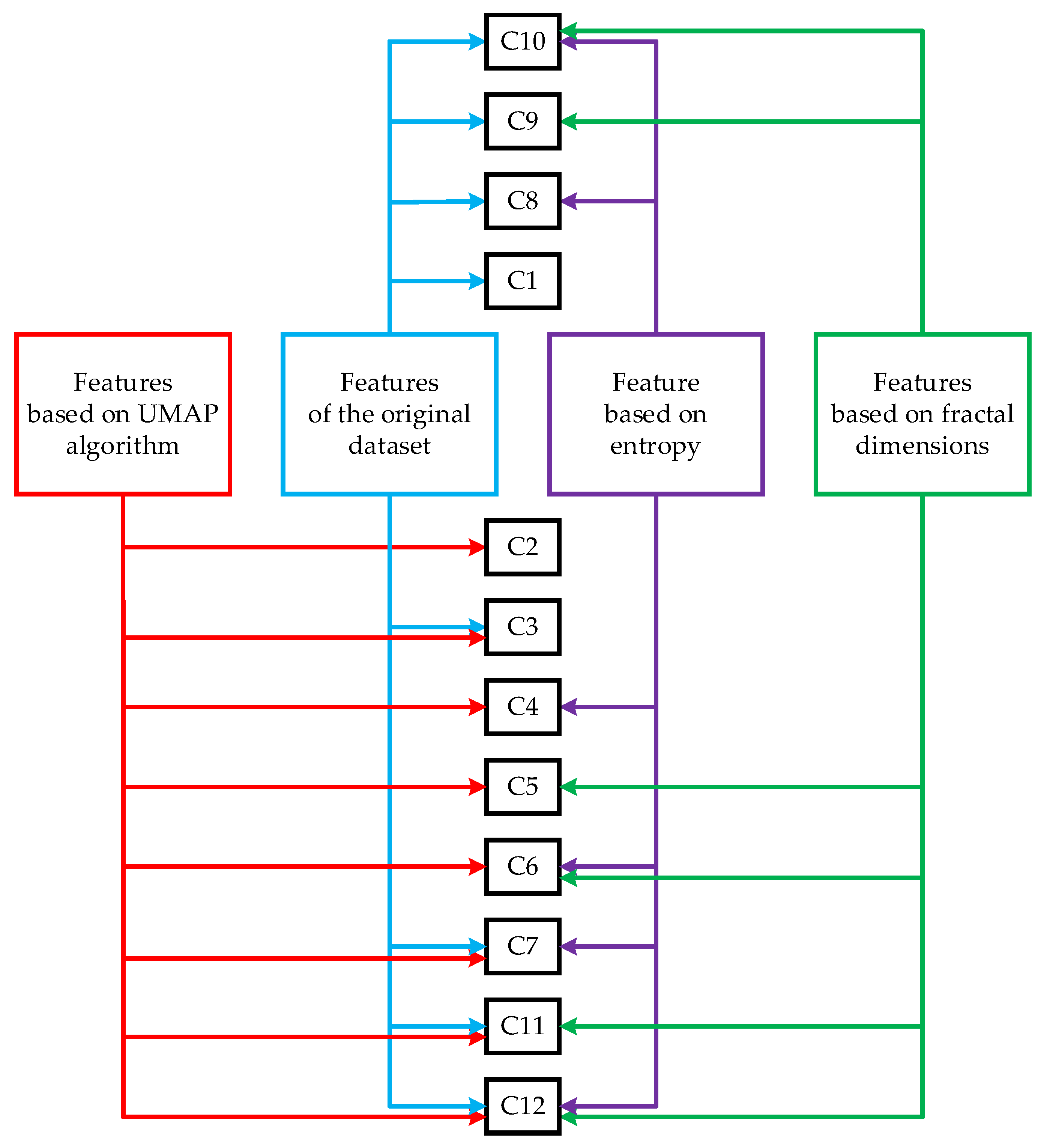
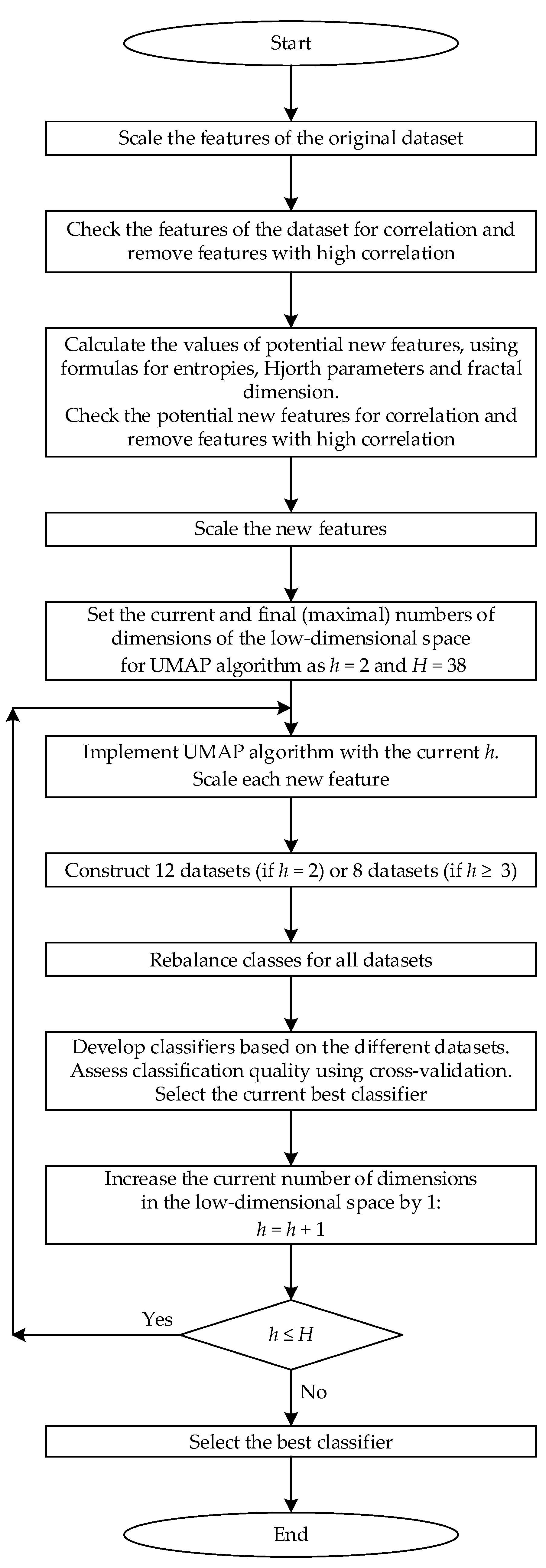
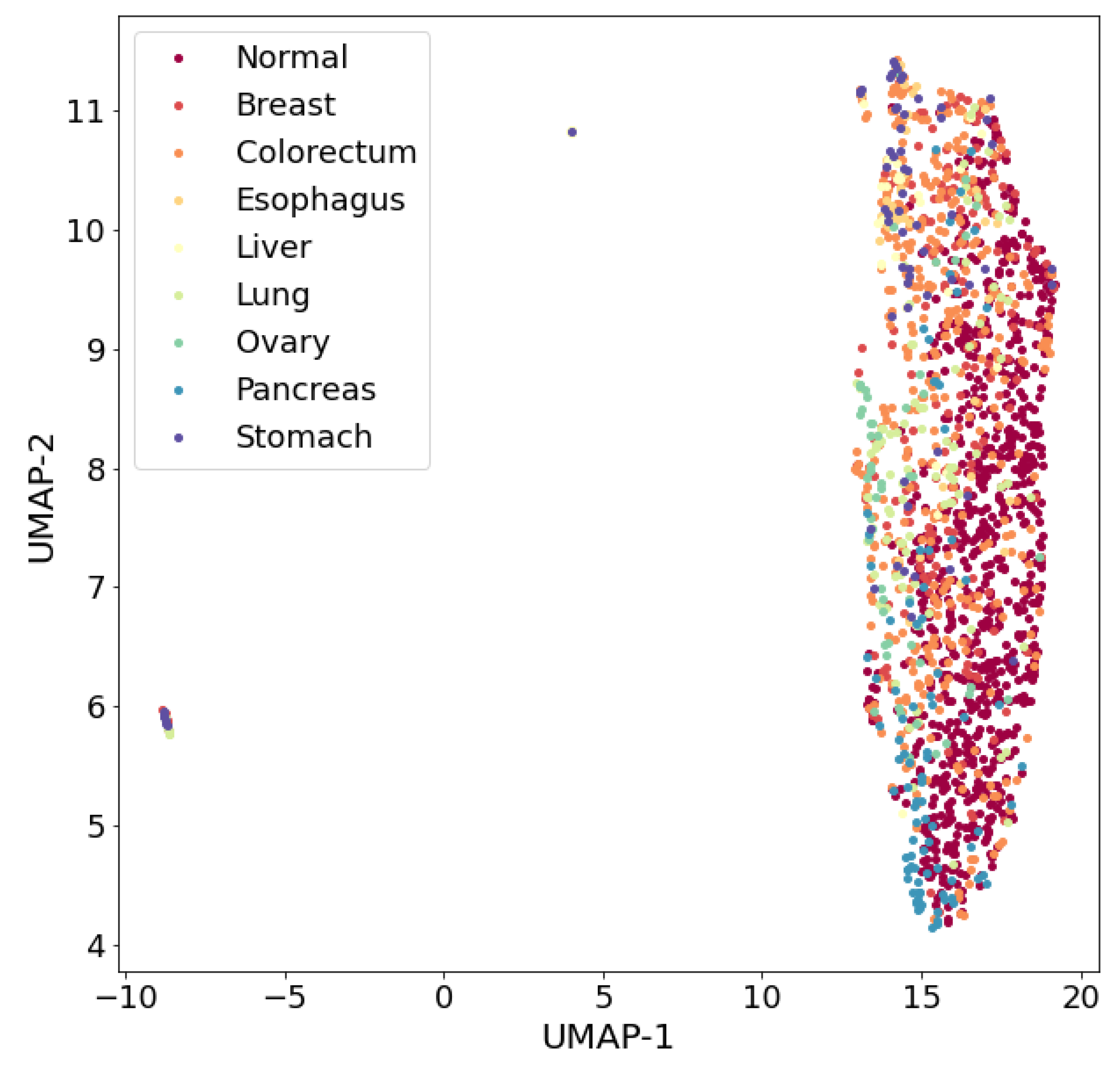
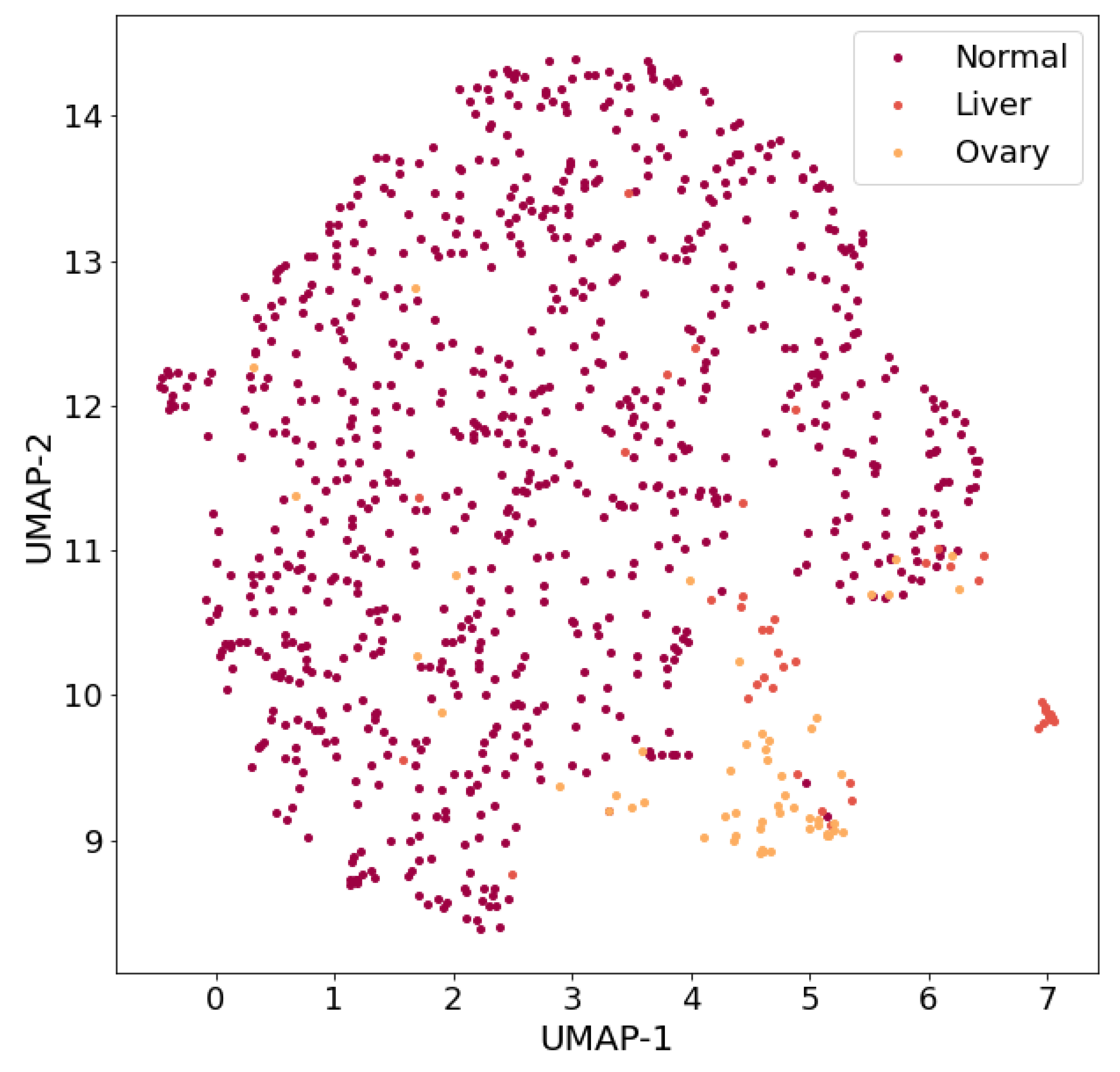
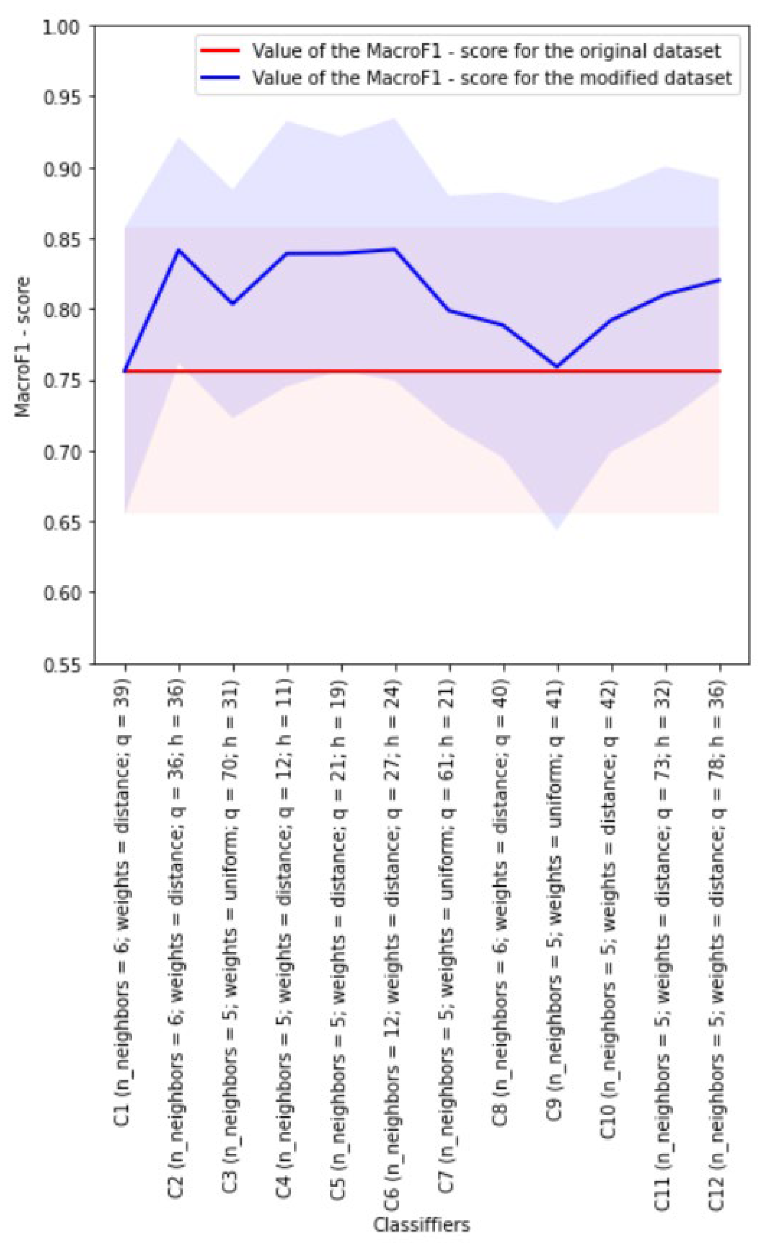
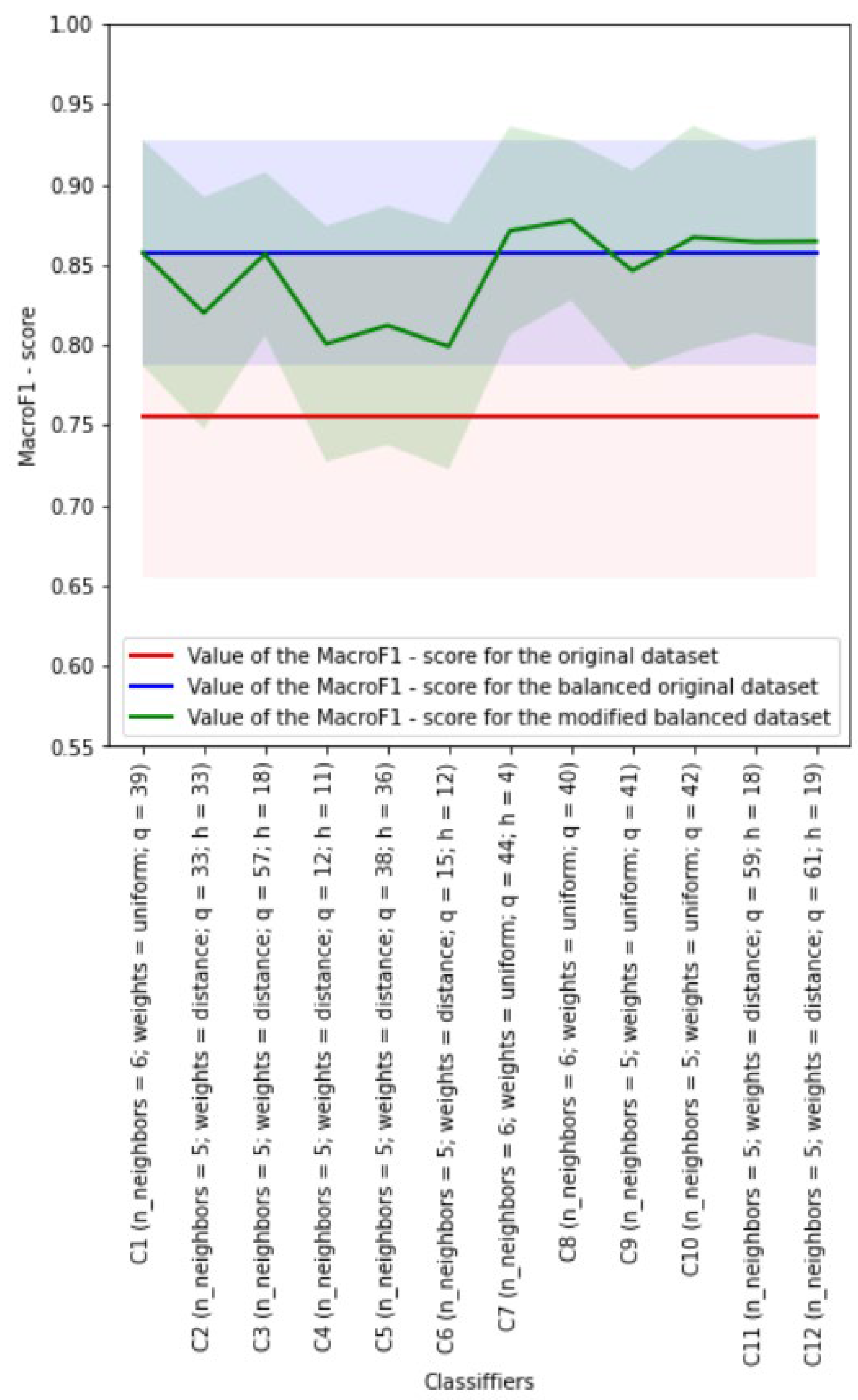
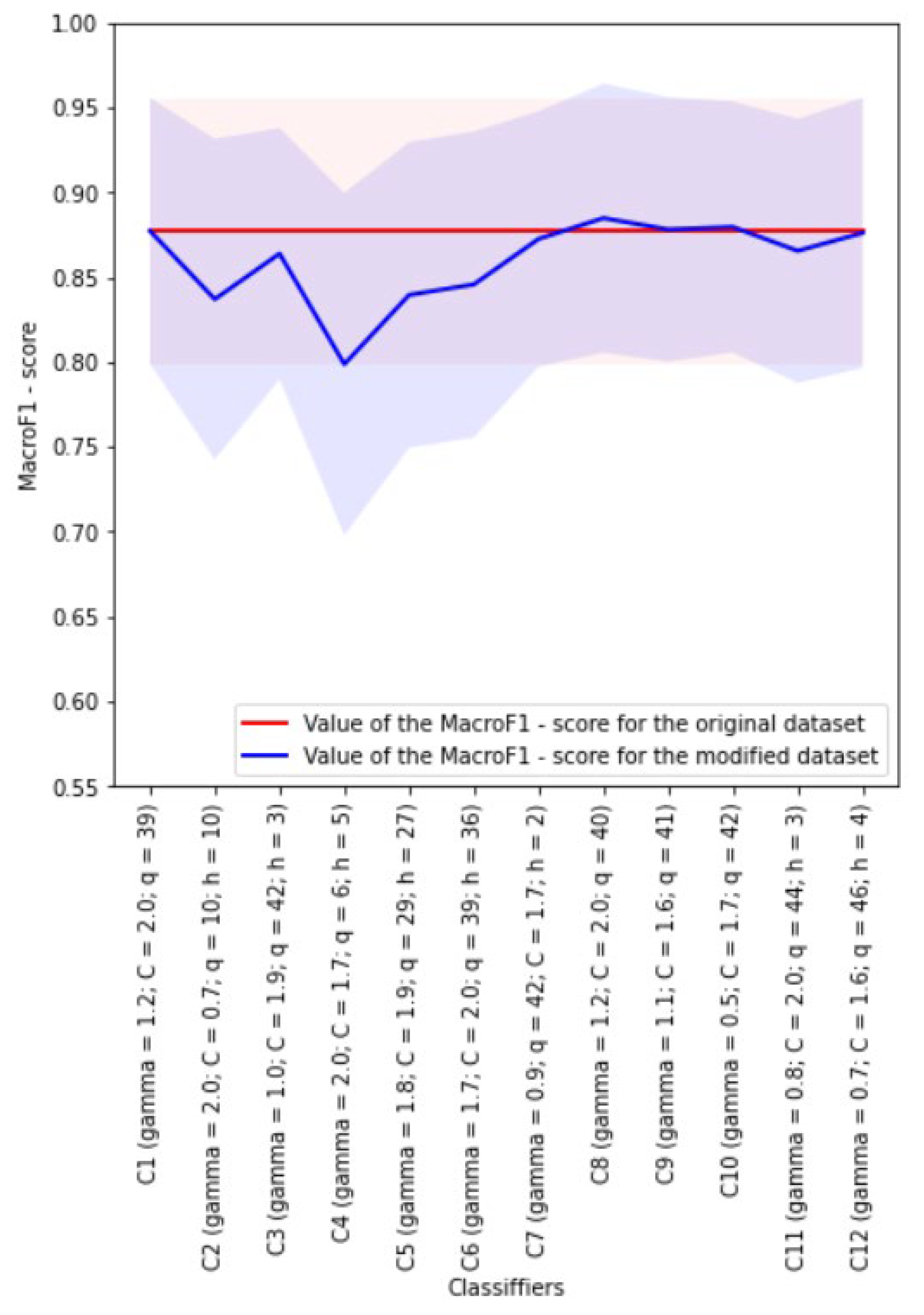
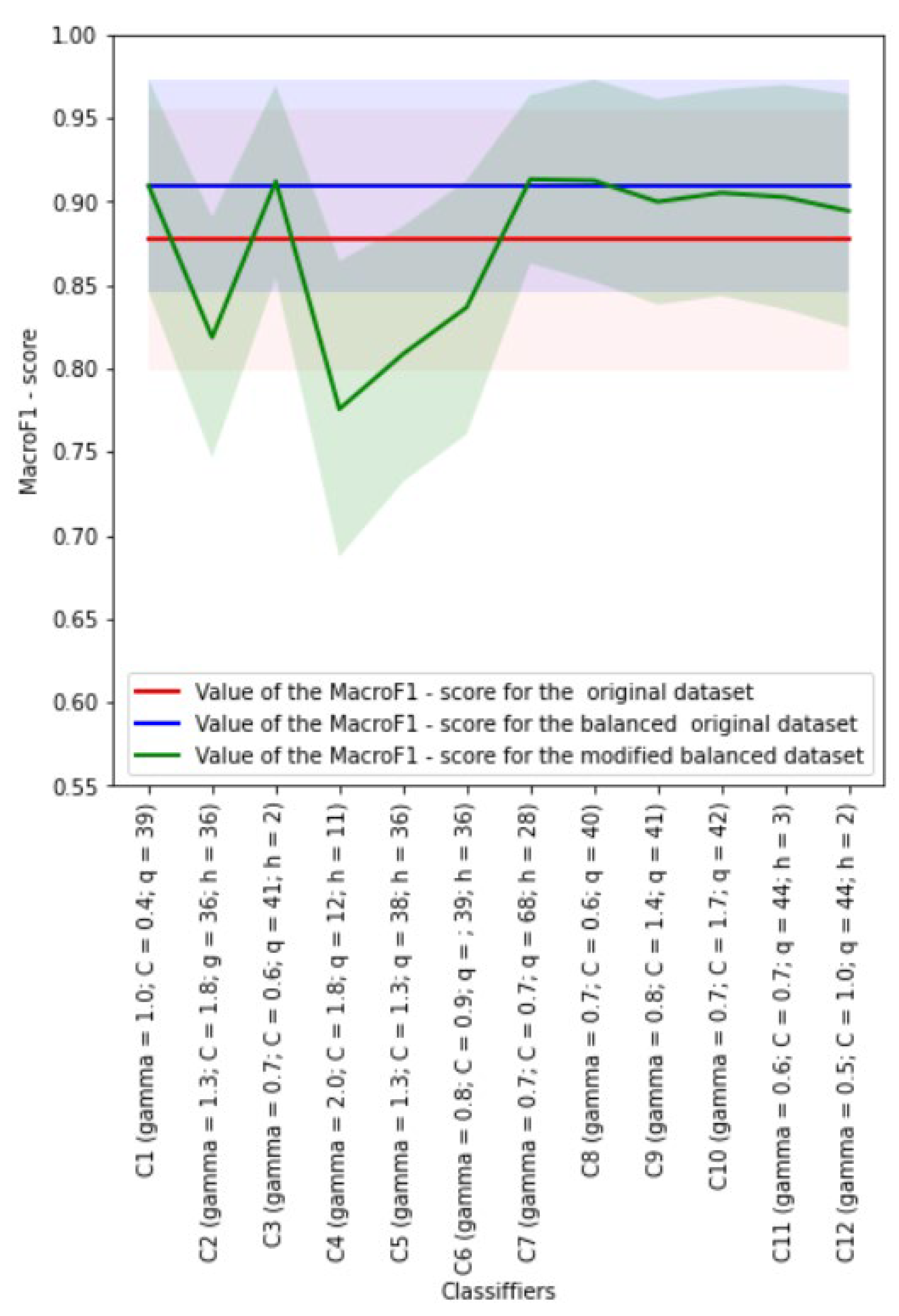