Article

A Robust Sphere Detection in a Realsense Point Cloud by USING Z-Score and RANSAC

by
Luis-Rogelio Roman-Rivera
*,†,
Jesus Carlos Pedraza-Ortega
,
Marco Antonio Aceves-Fernandez
,
Juan Manuel Ramos-Arreguín
,
Efrén Gorrostieta-Hurtado
and
Saúl Tovar-Arriaga
Facultad de Ingeniería, Universidad Autónoma de Querétaro, Cerro de las Campanas S/N, Querétaro 76010, Mexico
*
Author to whom correspondence should be addressed.
These authors contributed equally to this work.
Mathematics 2023, 11(4), 1023; https://doi.org/10.3390/math11041023
Submission received: 22 December 2022 / Revised: 11 February 2023 / Accepted: 15 February 2023 / Published: 17 February 2023
(This article belongs to the Special Issue Advances in Computer Vision and Machine Learning)

Abstract

:
Three-dimensional vision cameras, such as RGB-D, use 3D point cloud to represent scenes. File formats as XYZ and PLY are commonly used to store 3D point information as raw data, this information does not contain further details, such as metadata or segmentation, for the different objects in the scene. Moreover, objects in the scene can be recognized in a posterior process and can be used for other purposes, such as camera calibration or scene segmentation. We are proposing a method to recognize a basketball in the scene using its known dimensions to fit a sphere formula. In the proposed cost function we search for three different points in the scene using RANSAC (Random Sample Consensus). Furthermore, taking into account the fixed basketball size, our method differentiates the sphere geometry from other objects in the scene, making our method robust in complex scenes. In a posterior step, the sphere center is fitted using z-score values eliminating outliers from the sphere. Results show our methodology converges in finding the basketball in the scene and the center precision improves using z-score, the proposed method obtains a significant improvement by reducing outliers in scenes with noise from 1.75 to 8.3 times when using RANSAC alone. Experiments show our method has advantages when comparing with novel deep learning method.

1. Introduction

RGB-D cameras have become a common sensor in the area of computer vision [1,2], and the popularity started with the Microsoft Kinect output on their Xbox video game console, when the camera could be used on a personal computer, scientists started taking advantage of it for research [3]. This type of camera produces, as data output, a color image and an depth image, both images describing the scene that is captured on camera. Currently, there are different brands and models of RGB-D cameras, and it is common for different cameras to offer different characteristics and limitations [4]. Recently, this type of camera has been embedded in mobile devices as in [5] popularizing the technology and use of 3D point clouds. Some formats for saving 3D point clouds are the XYZ format and the PLY format, where spatial information is included describing each point in three dimensions and sometimes metadata, such as color, can be included. These files can vary in size and density of points and these depend mostly on the camera that is being used to generate such files, thousands of points can be found in a scene captured in a single shot, and, generally, the complexity of the processing of this information is increased proportionally with the quality of the camera and of the information it produces, the greater the detail, the greater point density. Novel methods can be found that use this type of information to solve problems in different fields, for example, in 3D reconstruction [6,7], simultaneous localization and mapping (SLAM) as in [8,9], navigation [10], object detection [11], mapping urban buildings [12], recovering building geometries [13,14], indoor scene reconstruction [7,15], computer vision as face recognition [16], segmentation with background removal [17], recognition tasks in robotics using scene modeling [18], navigation in agriculture [19], pedestrian detection [11], augmented reality (AR) [20], computer-assisted surgery [21], 3D navigation for pedestrians and robots [22], ADAS (advanced driving assistance systems) [23], uncrewed aerial vehicles (UAVs) navigation [24], autonomous driving [25], body tracking [26], and RGB-D Multi-Camera Pose Estimation for 3D Reconstruction [27]. There are different sets of data or databases that are compiled and organized to facilitate the research paper using information from different scenarios represented in 3D point clouds [28]. All of the mentioned applications use precise calibration parameters. In order to match the layers of color and depth, it is necessary to obtain the orientation and relative position between both layers of information (color and depth).
Object detection in 3D point clouds is commonly used to initiate subsequent processes, such as calibration of cameras [29], point cloud registration [30], clustering of objects, and 3D point cloud compression, spheres, cones, and cylinders are used as geometric objects due to the simplicity of being represented and/or modeled mathematically [31,32]. Random Sample Consensus (RANSAC) is a stochastic method, which uses samples producing specific parameters to be adjusted in a cost function and then lists the best proposals or candidates for solution [33], RANSAC has shown promising results locating geometric primitives in point clouds in three dimensions [34], as such can be adapted in the search for specific parameters and can speed up the time due to its stochastic nature.
Sphere detection is used in camera calibration [31], many approaches convert 3D data to 2D images as in [32], then use circle and ellipse detection to find circumferences in the 2D data and later translate coordinates from 2D to 3D to locate the sphere object in the 3D data. Furthermore, there are classical options as Hough Voting still being used [35,36], and deep learning approaches as in [37,38] to locate objects with a circular shape, novel approaches using deep learning allow to locate objects in complex scenes. Some previous methods use RANSAC to find and fit the sphere, nevertheless unlike the method proposed in [32] a background subtraction is required to limit the search space. In the work of [34], to locate a sphere normal vectors are required and tolerances on the angles of the normals are used as a second acceptance criteria for the sphere to be accepted as a RANSAC candidate, in our proposal only tolerance is used on the distance as a criteria for acceptance as a RANSAC candidate.
A method to locate spheres with a known size directly in 3D point clouds is proposed, our experiments show advantages when using 3D data directly against converting the 3D point cloud to a 2D image and then use 2D methods. Some areas of application of the proposed method are RGB-D camera calibration, RGB-D Multi-Camera Pose Estimation, 3D registration, 3D navigation.
Our strategy shows the following features:
  • Three-dimensional data are used directly by our method.
  • Sphere size is used as a pattern to be searched.
  • The proposed method allows to find the sphere in complex scenes with multiple objects and textures.
  • No additional conversions are needed to detect the sphere.
  • It is robust to outliers.

2. Materials and Methods

2.1. Computer Equipment, Programming Language
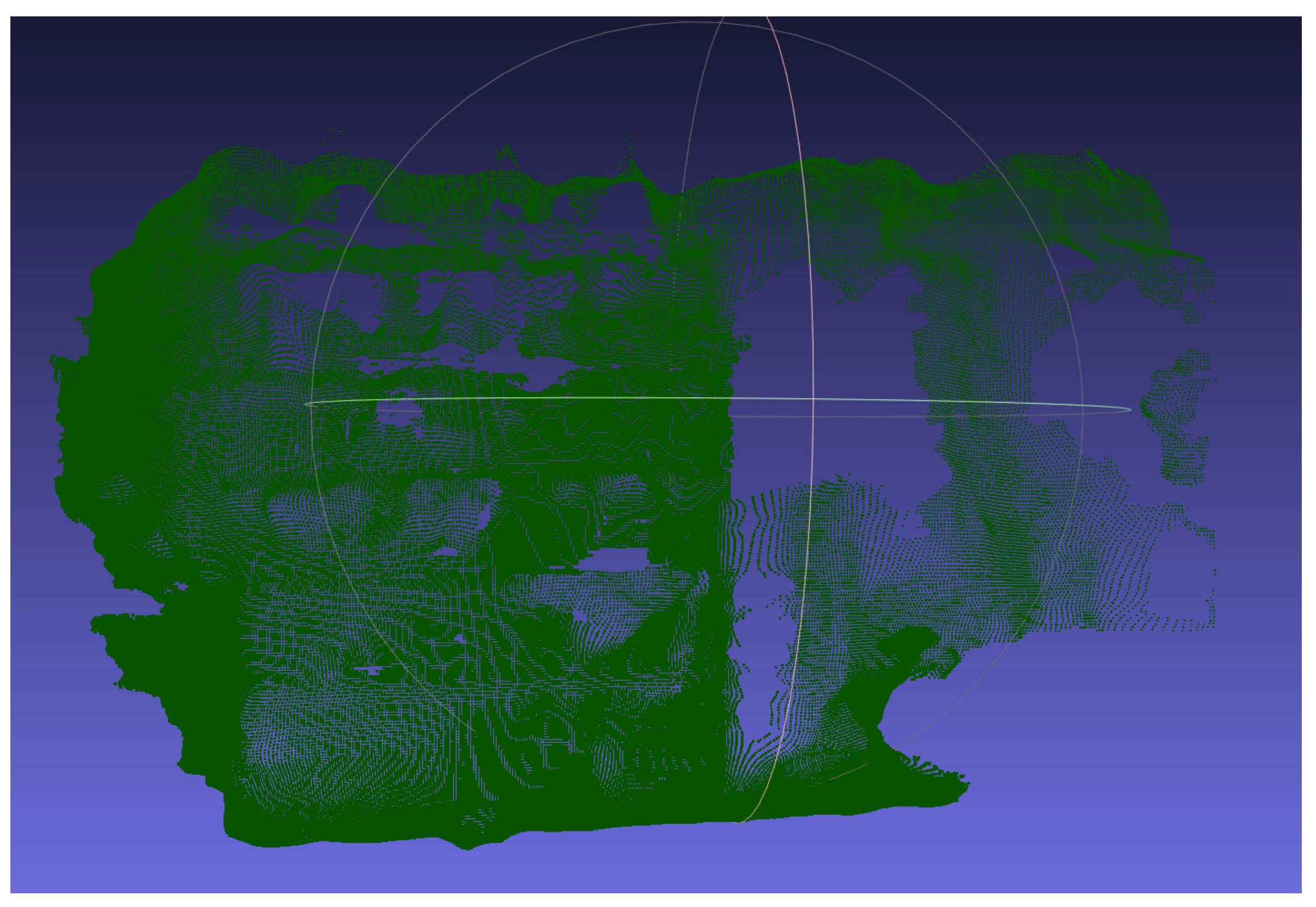
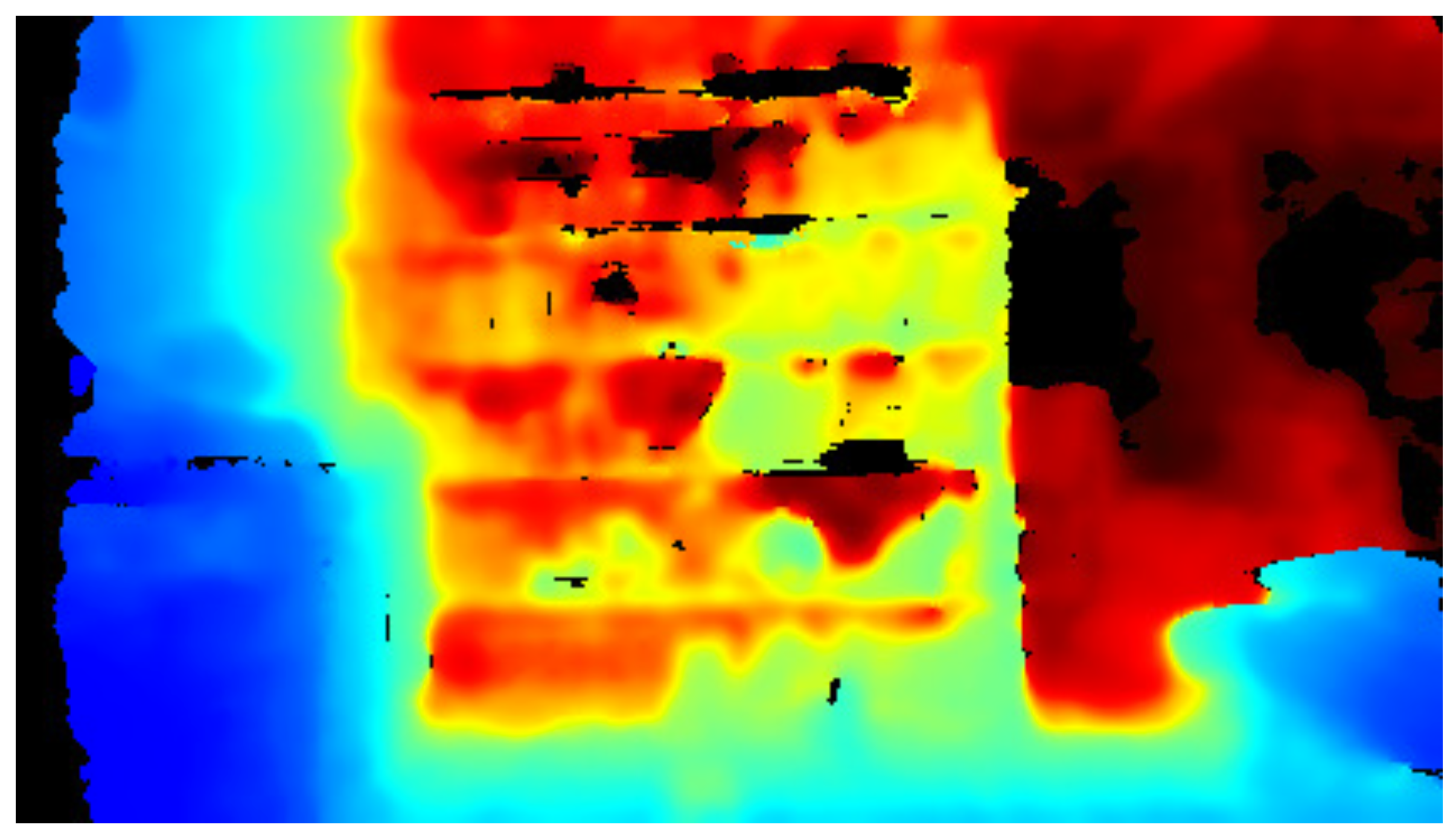
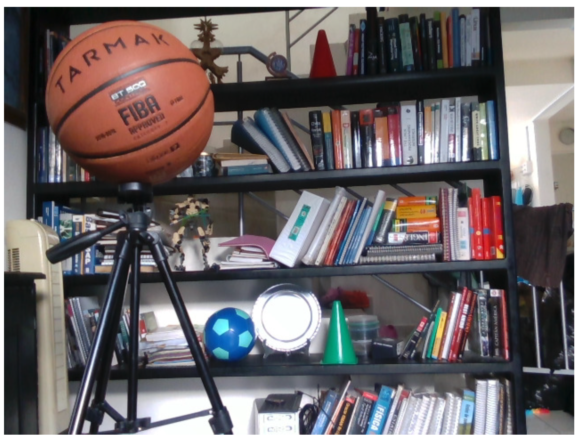
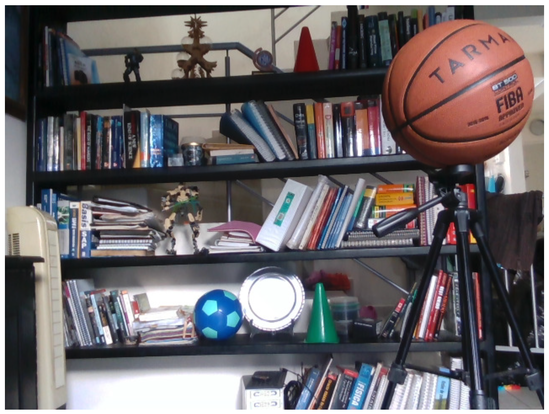
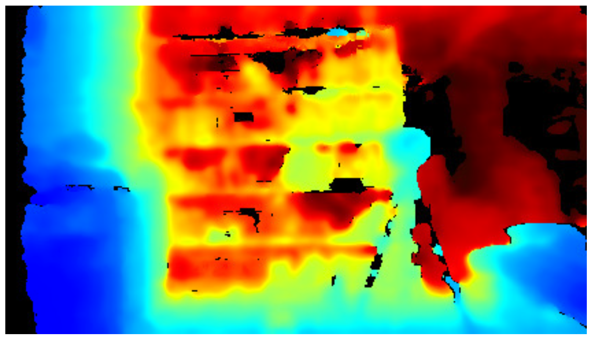
In this work, a personal computer with the following features, AMD Ryzen 5600x Processor with 6 cores, 12 processing threads, 3.7 GHz, 32 MB Cache L3, 3 MB Cache L2, 32 GB RAM, NVIDIA graphics card GeForce RTX 3060 TI with 8GB GDDR6 Memory, 4864 CUDA kernels, Ubuntu 20.04.2 LTS OS, Containers Docker 19.03.8, CUDA driver version 11.2. Python 3.9 as a programming language. Additionally, a MacBook air (Retina 13-inch, 2020) laptop was used with 1.1 GHz Quad-Core Intel Core i5 CPU, 8 GB RAM and integrated graphics card Intel Iris Plus Graphics 1536 MB, operating system Mac OS Big Sur 10.13 Beta and Python 2.9. All experiments will be run by exchanging the environment between the personal computer and the laptop, it was used Meshlab to visualize PLY files.
During all experiments, we use an Intel Realsense D435 with the specifications in Table 1.

2.2. RGB-D Camera

A camera was used during the capture of the scenes. RGB-D Intel RealsenseTM D435 with the following characteristics Table 1. The depth images produced by the camera in experiments contain 101,760 points in 3D for each capture of a scene. The scene in the depth image is represented in integers and has to be converted by a value of 0.001 that is configured from the factory in the RGB-D camera as depth unit. Integer values within the depth image were converted to meters using Equation (1).
Z ( I i j ) i j = I i j × 0.001
Additionally, a projection is made from 2D coordinates to coordinates in 3D by the following Equation (2)
X ( I i j ) i j = ( i c x ) / f x × 0.001 Y ( I i j ) i j = ( i c y ) / f y × 0.001
Here, c x is the center of the sphere in the x-axes, c y is the center of the sphere in y-axes and f x is the focal length in x-axes and f y is the focal length in the y-axes, the 3D point cloud is represented with coordinates (x, y, z) and the dimensions are represented in meters with floating point numbers. The maximum and minimum value of depth depends directly of the scene captured and the characteristics of the RGB-D camera. Information contained in a ply file is shown in Figure 1 which is displayed through the Meshlab program, it is observed that all points in 3D are displayed in green and there is no clear distinction of the objects present in the scene, the structure of a bookcase is predominantly observed. In Figure 2, we can see more clearly the different layers of depth due to the representation in colors from blue to red with increasing distance from the RGB-D camera.
The shot of a scene by the camera is displayed RGB-D (Figure 1 and Figure 2). An attempt is made to capture objects at different distances in each experiment.

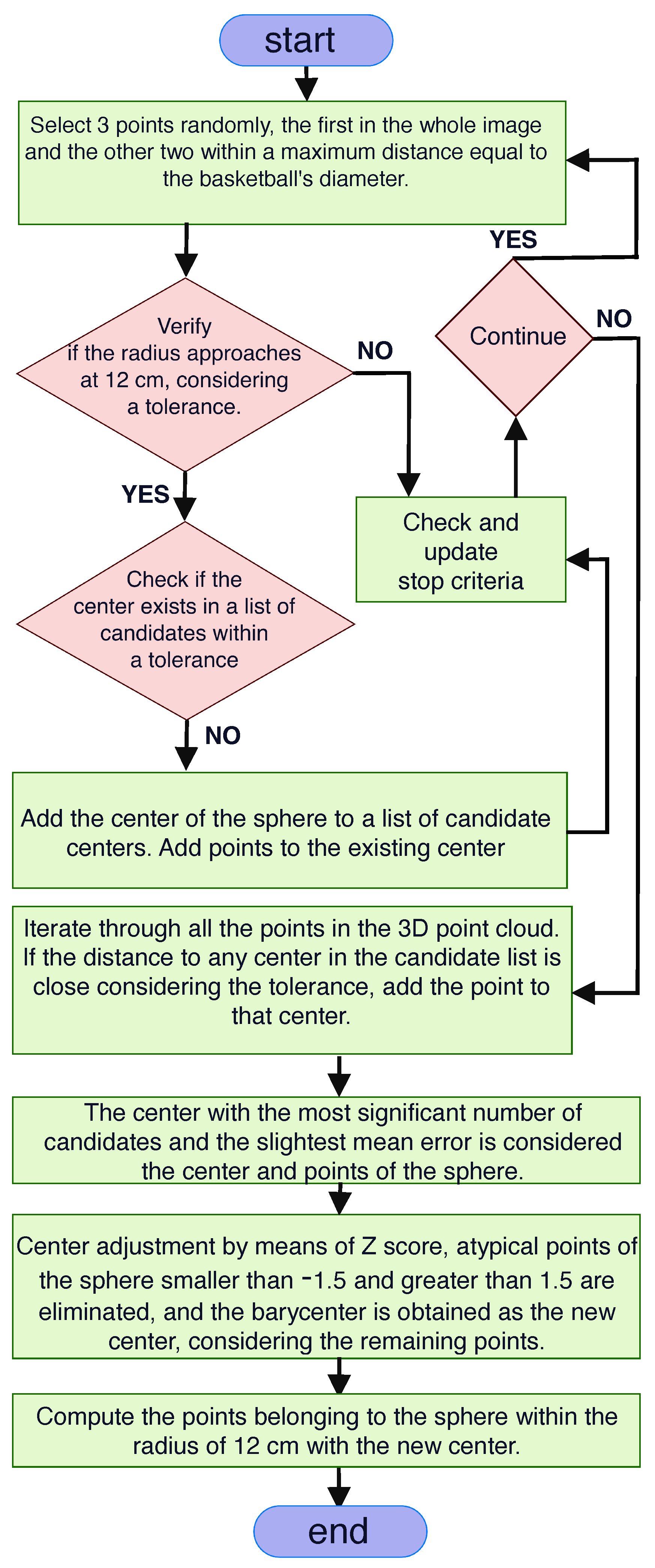
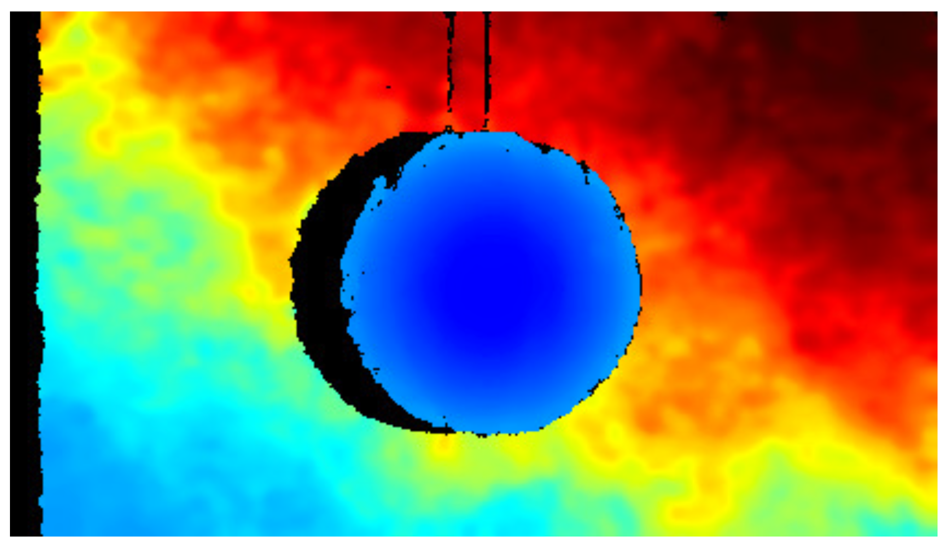
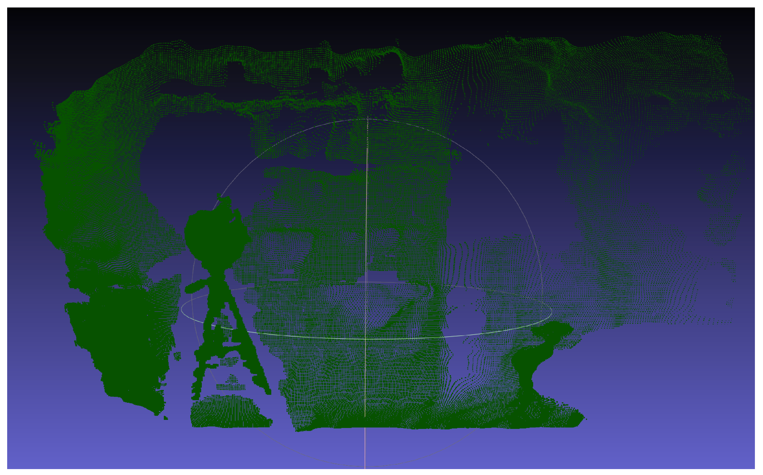
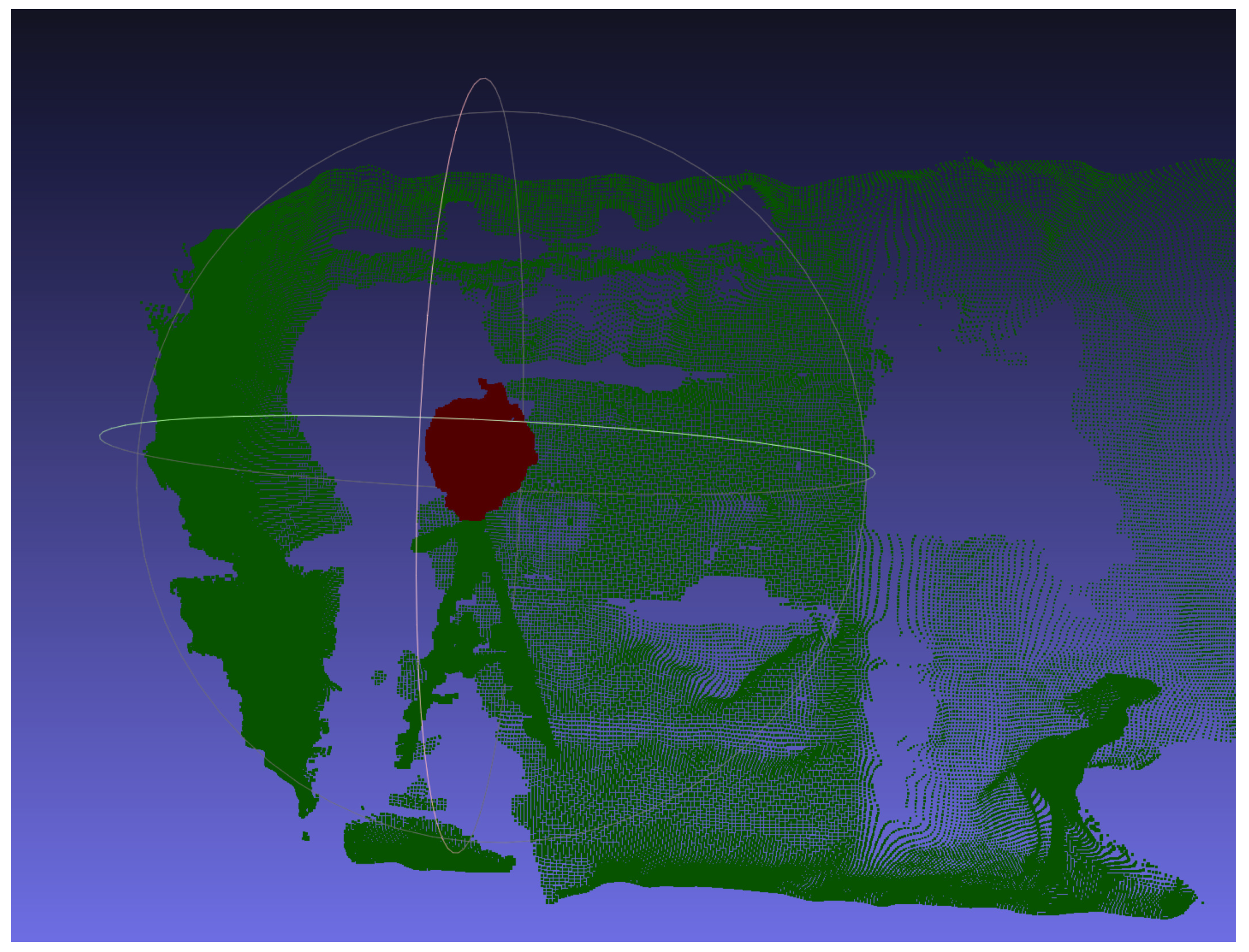
2.3. Model to Represent the Sphere with a Known Size
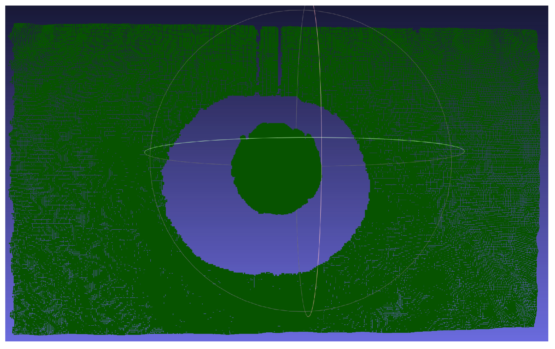
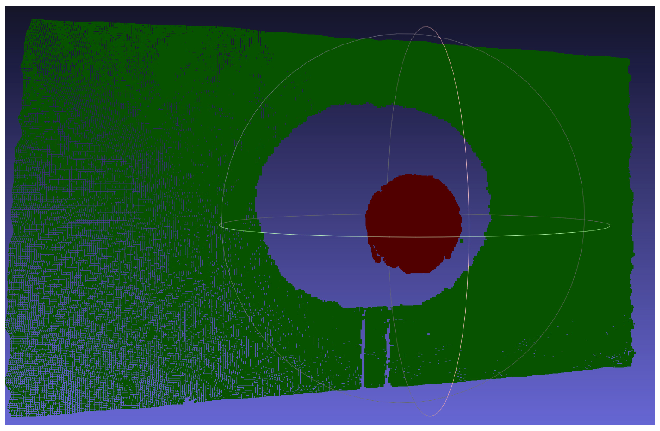
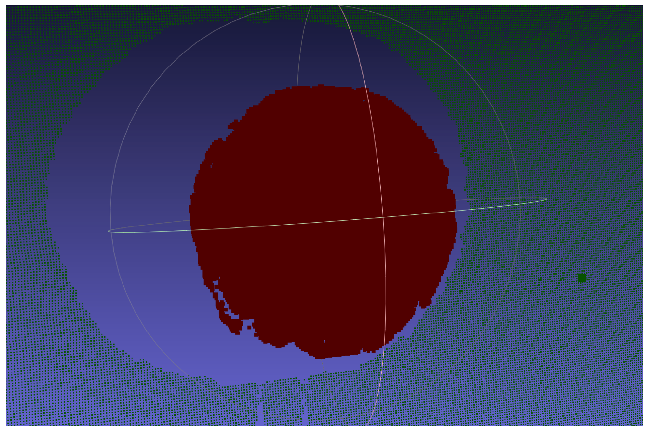
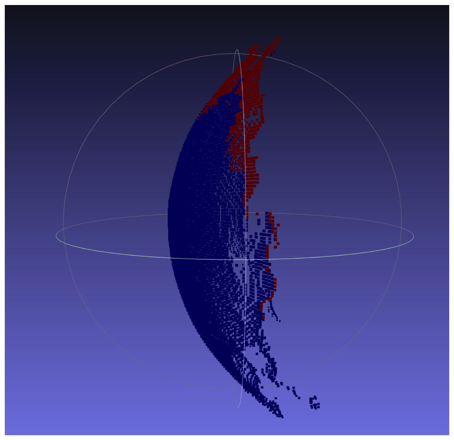
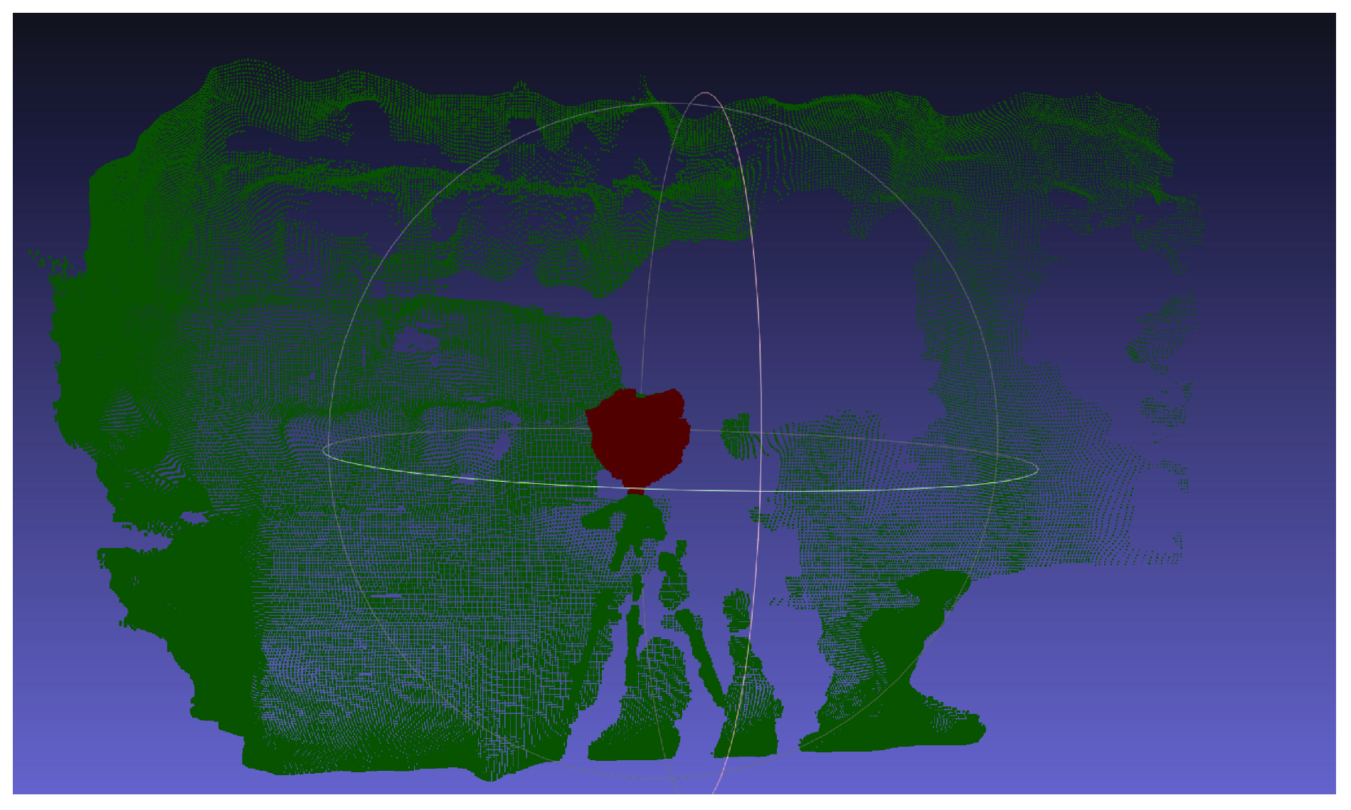
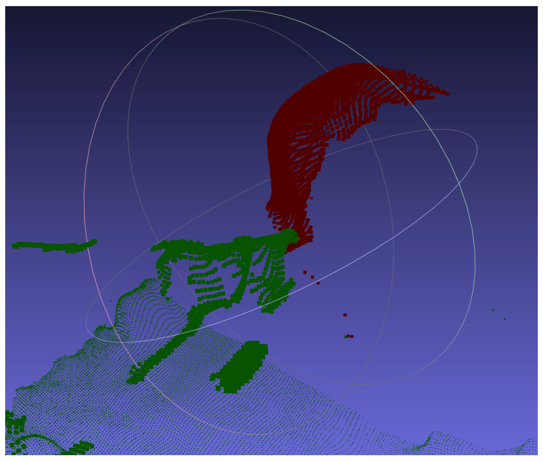
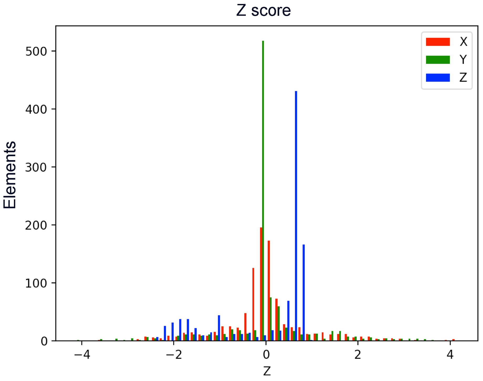
An equation is used to model a sphere where on its surface we find three different points x i , y i , z i with a common center or with coordinates a , b , c :
O = ( a , b , c )
r 2 = ( x i a ) 2 + ( y i b ) 2 + ( z i c ) 2
here, r is the radius of the sphere. Expanding right side of Equation (4) for at least 2 different points:
r 2 = x 1 2 2 x 1 a + a 2 + y 1 2 2 y 1 b + b 2 + z 1 2 2 z 1 c + c 2 r 2 = x 2 2 2 x 2 a + a 2 + y 2 2 2 y 2 b + b 2 + z 2 2 2 z 2 c + c 2
Simplifying for two different points:
r 2 = x 1 2 2 x 1 a + a 2 + y 1 2 2 y 1 b + b 2 + z 1 2 2 z 1 c + c 2 r 2 = x 2 2 2 x 2 a + a 2 + y 2 2 2 y 2 b + b 2 + z 2 2 2 z 2 c + c 2
Then:
x 1 2 2 x 1 a + y 1 2 2 y 1 b + z 1 2 2 z 1 c = x 2 2 2 x 2 a + y 2 2 2 y 2 b + z 2 2 2 z 2 c x 1 2 x 2 2 2 x 1 a + 2 x 2 a + y 1 2 y 2 2 2 y 1 b + 2 y 2 b + z 1 2 z 2 2 2 z 1 c + 2 z 2 c = 0 x 1 2 x 2 2 + 2 a ( x 2 x 1 ) + y 1 2 y 2 2 + 2 b ( y 2 y 1 ) + z 1 2 z 2 2 + 2 c ( z 2 z 1 ) = 0
Expanding the Equation (4) for three different points:
r 2 = ( x 1 a ) 2 + ( y 1 b ) 2 + ( z 1 c ) 2 r 2 = ( x 2 a ) 2 + ( y 2 b ) 2 + ( z 2 c ) 2 r 2 = ( x 3 a ) 2 + ( y 3 b ) 2 + ( z 3 c ) 2
then in Equation (8) each equation equals r so match in the following order:
( x 1 x c ) 2 + ( y 1 y c ) 2 + ( z 1 z c ) 2 = ( x 2 x c ) 2 + ( y 2 y c ) 2 + ( z 2 z c ) 2 ( x 3 x c ) 2 + ( y 3 y c ) 2 + ( z 3 z c ) 2 = ( x 1 x c ) 2 + ( y 1 y c ) 2 + ( z 1 z c ) 2 ( x 3 x c ) 2 + ( y 3 y c ) 2 + ( z 3 z c ) 2 = ( x 2 x c ) 2 + ( y 2 y c ) 2 + ( z 2 z c ) 2
The 3D Point Coordinates 1 = 3D Point Coordinates 2, 3D Point Coordinates 3 = 3D Point Coordinates 1, 3D Point coordinates 3 = 3D Point Coordinates 2, and using Equation (7) developing the system of Equation (9) we obtain:
2 a ( x 2 x 1 ) + 2 b ( y 2 y 1 ) + 2 c ( z 2 z 1 ) + x 1 2 x 2 2 + y 1 2 y 2 2 + z 1 2 z 2 2 = 0 2 a ( x 3 x 1 ) + 2 b ( y 3 y 1 ) + 2 c ( z 3 z 1 ) + x 1 2 x 3 2 + y 1 2 y 3 2 + z 1 2 z 3 2 = 0 2 a ( x 3 x 2 ) + 2 b ( y 3 y 2 ) + 2 c ( z 3 z 2 ) + x 2 2 x 3 2 + y 2 2 y 3 2 + z 2 2 z 3 2 = 0
simplifying Equation (10) and rearranging in the form Ax = b we obtain:
2 x 2 x 1 2 y 2 y 1 2 z 2 z 1 2 x 3 x 1 2 y 3 y 1 2 z 3 z 1 2 x 3 x 2 2 y 3 y 2 2 z 3 z 2 a b c = x 2 2 x 1 2 + y 2 2 y 1 2 + z 2 2 z 1 2 x 3 2 x 1 2 + y 3 2 y 1 2 + z 3 2 z 1 2 x 3 2 x 2 2 + y 3 2 y 2 2 + z 3 2 z 2 2
Then:
x 2 x 1 y 2 y 1 z 2 z 1 x 3 x 1 y 3 y 1 z 3 z 1 x 3 x 2 y 3 y 2 z 3 z 2 a b c = 1 / 2 x 2 2 x 1 2 + y 2 2 y 1 2 + z 2 2 z 1 2 x 3 2 x 1 2 + y 3 2 y 1 2 + z 3 2 z 1 2 x 3 2 x 2 2 + y 3 2 y 2 2 + z 3 2 z 2 2
the Equation (12) can be solved to calculate the radius by three different points on the surface of the sphere.

2.4. Z-Score

To remove outliers in the set of points that are considered as part of the sphere the punctuation is used Z [40], to remove values below a defined threshold from −1.5 and above 1.5.
z = ( X i X ¯ ) / σ
where X i is the measured value, X ¯ is the average of the values and σ is the standard deviation.

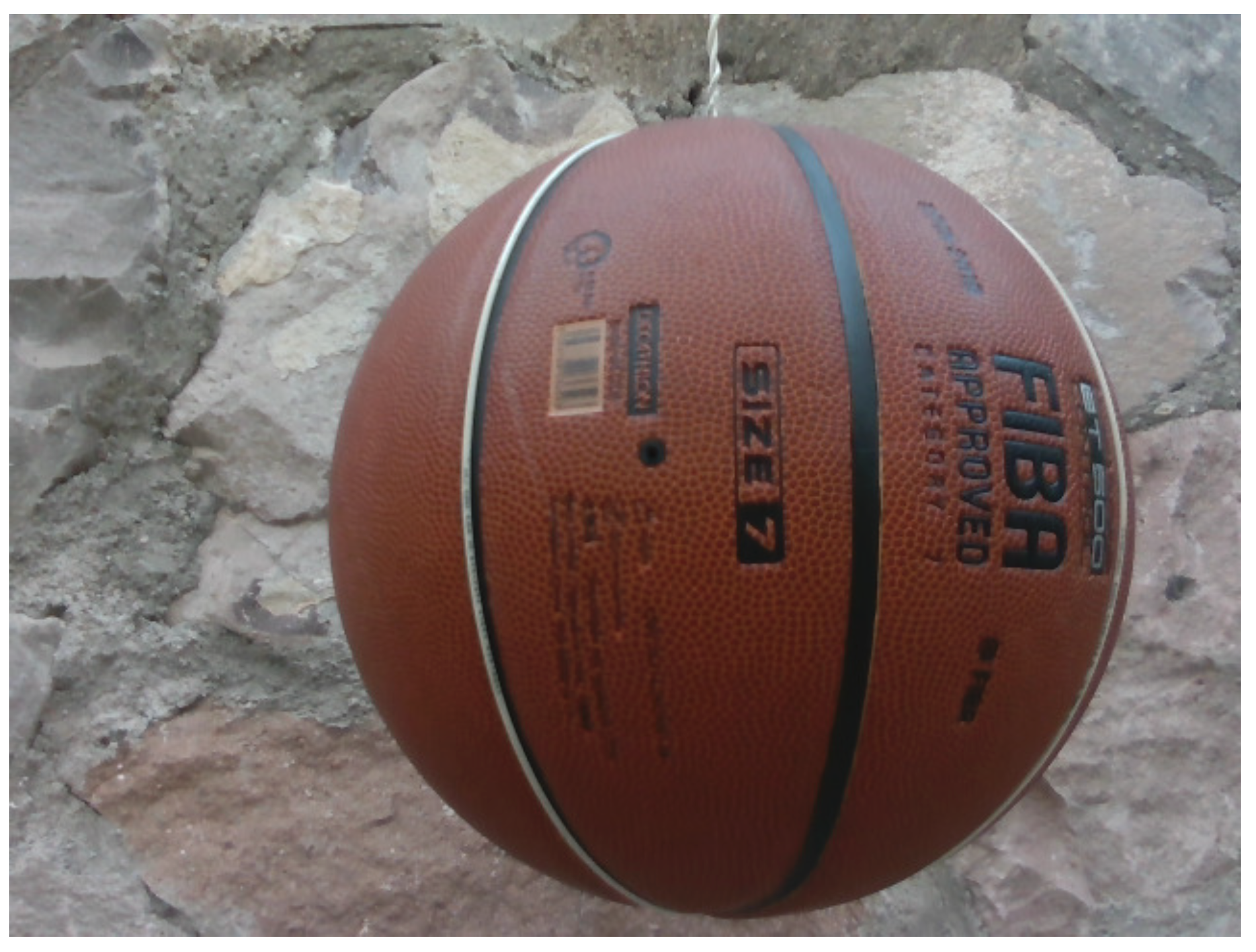
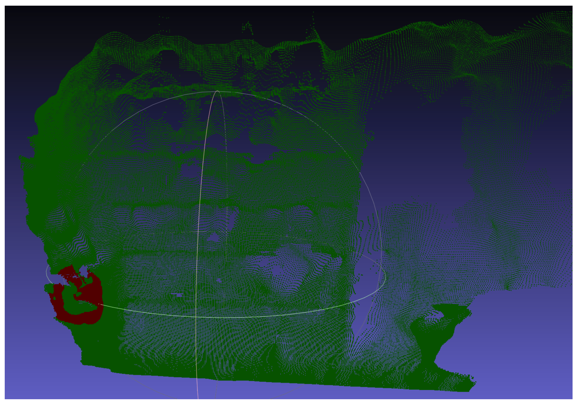
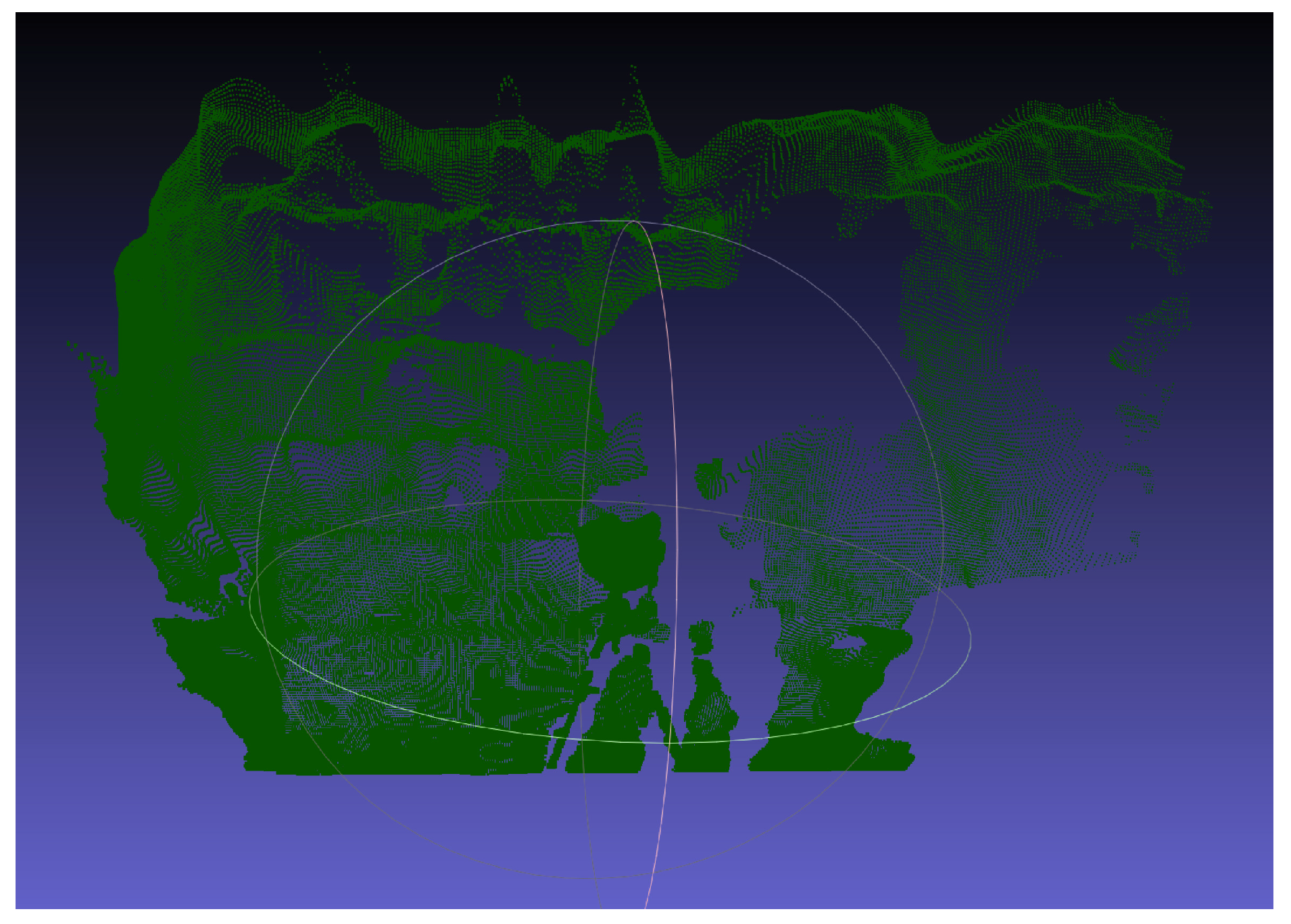
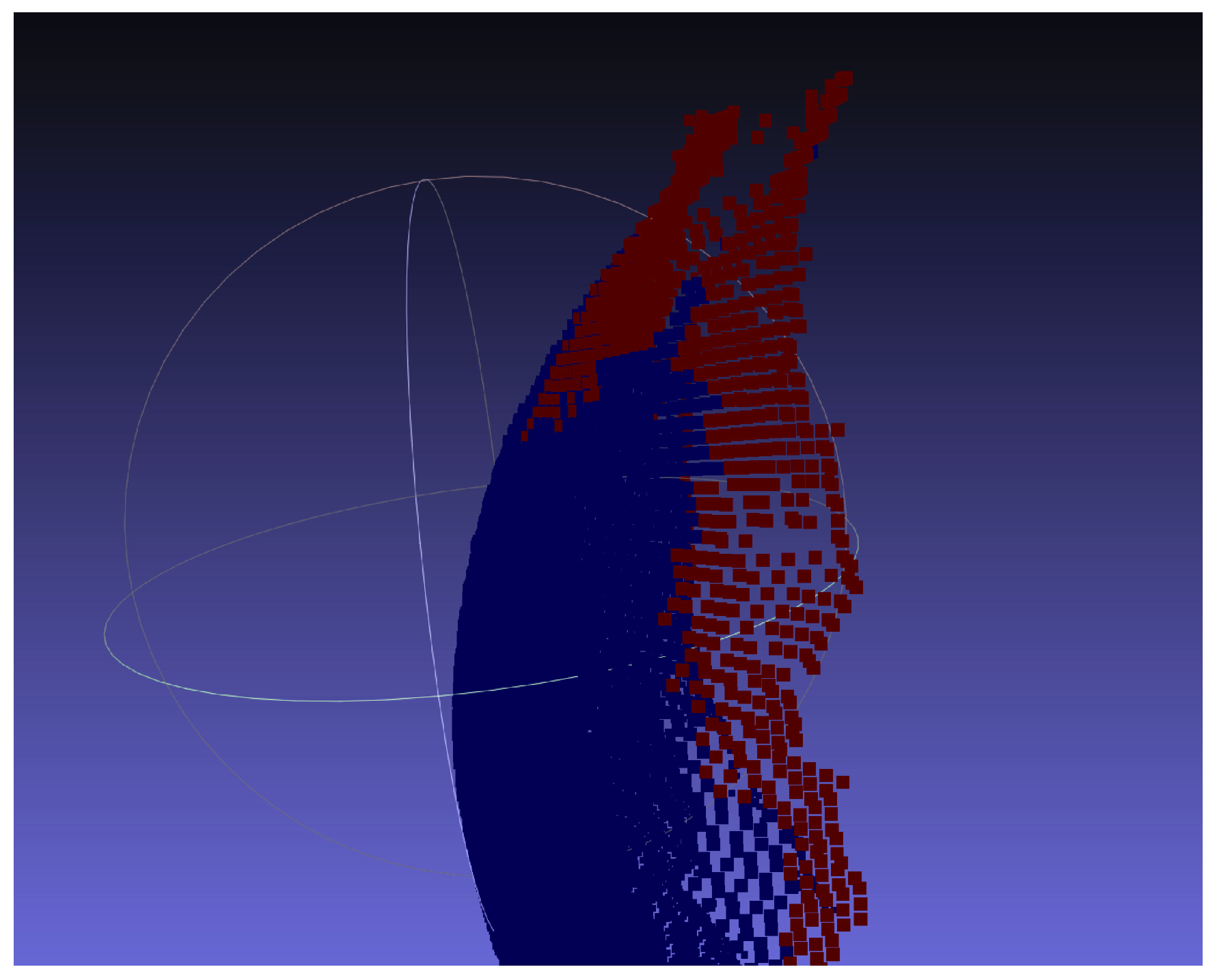
2.5. Basketball and RANSAC Method

In the algorithm shown in the flowchart (Figure 3), as a first step, three points are selected randomly from the 3D point cloud, we obtain the center with Equation (11) and later the radius with Equation (4), as step two, check that the radius is within a tolerance of ϵ = 1 cm close to the radius of the ball of basketball with a radius of 12 cm. If it is within tolerance checks that the center exists in a list of candidate centers. If it exists, the points are added to the center of the list. If the center does not exist, a new center is added. along with its points on the surface of the sphere to the list. If a radius is not found within tolerance, check and update the stop condition which can be a limit of iterations, in the experiment a thousand iterations were used as a limit. If the stop condition is still not reached, three new candidates randomly and it starts over in the first step. If the stop condition is reached, iterates through all the points in the point cloud in 3D and check distances to registered centers, if centers are found within tolerance, each point evaluated is added to the list of whose center it corresponds.
Once the classification of the points to their centers is finished corresponding, the list is sorted and the center is selected with the greatest number of points and the least error with respect to the tolerance in the measure of the radius of the sphere. Subsequently, an adjustment of the center of the sphere is made, for this, it is used z-score or Z score, to eliminate outliers, eliminate data with Z-score less than −1.5 and greater tan 1.5, with the remaining values a barycenter is calculated and it is taken as the new center of the sphere, through which they are considered sphere points those points within the defined radius.

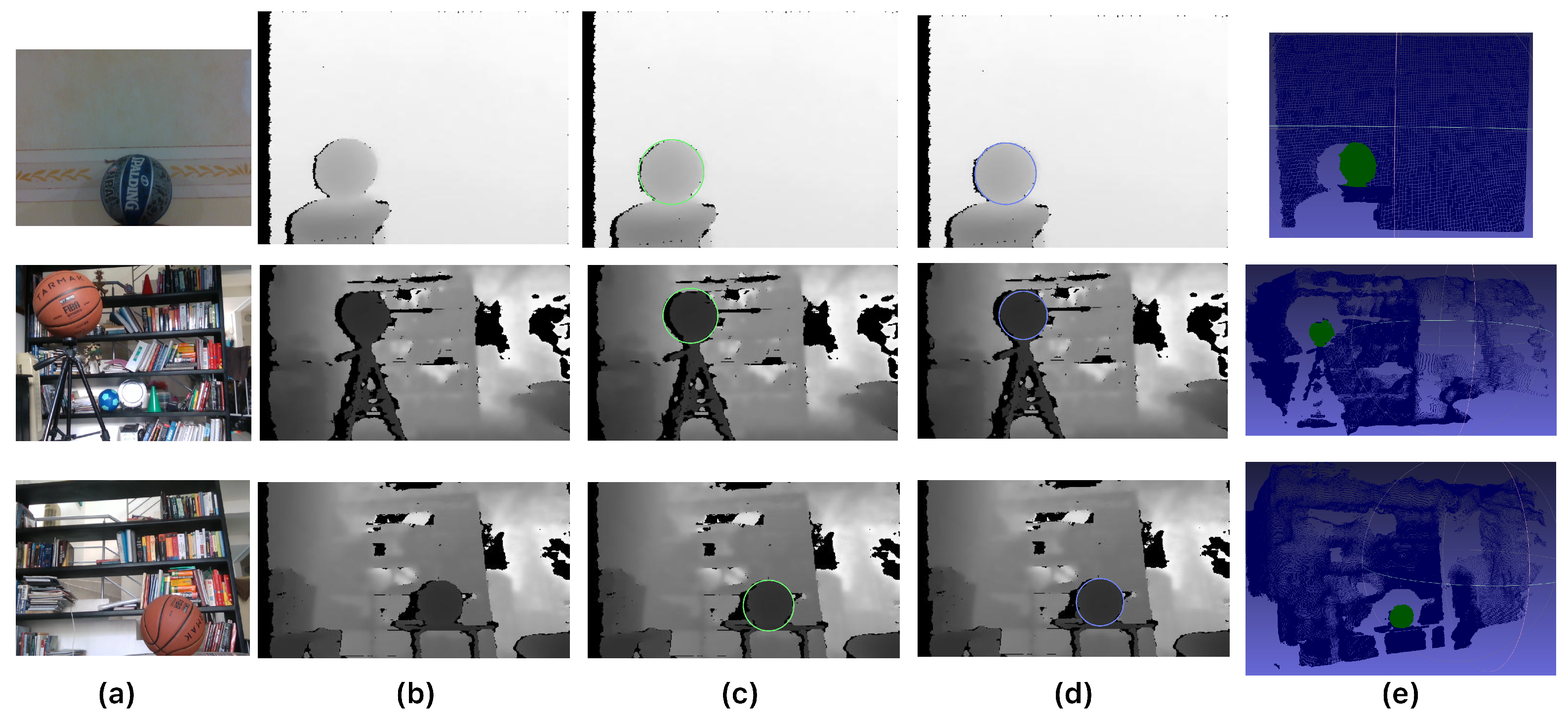
3. Experiments and Results

A standard size 7 basketball is used, with a circumference of approximately 35 cm and a radius of 12 cm as show in Figure 4. With a fixed radius, a tolerance of 1 cm and the RANSAC method can be integrated to adjust the system of Equations (11) by sampling three points in the 3D point cloud.
A scene with a relatively flat wall is selected to the bottom and a basketball is placed 25 cm from the realsense D435 camera, the image is captured in color or RGB (Red Green Blue, color image) as shown (Figure 4).
The depth of the same scene is captured by the realsense D435 camera, which is converted to a file PLY using Equations (1) and (2), the scene can be displayed in shades of color from blue to red as shown (Figure 5), and subsequently the PLY file is visualized with Meshlab (Figure 6).
The correct detection of the basketball is shown (Figure 7 and Figure 8) as a spherical geometry in a first experiment with good conditions in the scene where the soccer ball basketball is distinguished from the rest of the scene and is not occluded by other objects. The 3D points that belong to the surface of the ball are colored red and are distinguished from the other points in the scene.
The tolerance ϵ defines the number of outliers at locations near the surface of the sphere. In this example, a thousand iterations were used to search for on the entire image per iteration, in each experiment different candidate solution proposals are generated as the center of the sphere that is sought, different solutions, because there are different points that satisfy the proposed mathematical model Equation (11) within tolerance established, however the candidate with the highest number of points and whose radius approaches with less error to the known measure of 12 cm, is the selected solution using the RANSAC method. In this first experiment, the different candidates that are generated belong to the same object, so the center is very similar in all proposals, however, the method converges to the winning center.
The adjustment of the points of the sphere is carried out by means of the Z-score Equation (13), of the points that turn out to belong to the sphere with the winning center, minor points are removed to −1.5 and greater than 1.5, which are considered as values outliers, these values were selected by means of a heuristic based on a lower RMSE type error (Root mean square error). A new center is calculated by a centroid with the remaining points. seen in color red the points discriminated as outliers (Figure 9) using the Z-score and the dots in blue as the values within the sphere of radius 12 cm from the new center.
In a second experiment, an image is generated with the Realsense D435 camera of a scene with greater complexity to the first experiment, in whose middle part, in the middle part of the scene there is a bookcase with various objects, showing a brown basketball on a tripod, which is sought by the proposed method. The scene of the second experiment is shown (Figure 10).
A depth image of the scene is generated (Figure 10), which is converted to a PLY file using Equations (1) and (2), the PLY file is visualized with Meshlab (Figure 11).
The correct detection of the basketball is shown (Figure 12) as a spherical geometry. In this image there are outliers in places close to the surface of the sphere as it can be parts of the scene that correspond to the tripod where the ball rests. In this example we used 10,000 iterations searching the entire image, in each experiment different candidate solution proposals as the center of the sphere that is sought, different solutions are found because there are points that satisfy the proposed mathematical model Equation (11) within the established tolerance, however in this experiment the candidate with the largest number of points and whose radius approaches with a smaller error the measure known 12 cm is the solution selected by the RANSAC method.
It is observed that false positives can be obtained if the tolerance is higher and if the scene is sampled without enough frequency or considering a space away from the dimensions of the actual diameter of the ball 24 cm, as in (Figure 13) where the incorrect detection of certain points that satisfy the model mathematical to represent the sphere are showed, but that nevertheless they do not belong to the geometry being sought.
A scene is captured by increasing the distance of the ball basketball towards the camera in a third experiment considering multiple levels of depth as seen in the color image (Figure 14).
A difference in depth is observed with respect to the second experiment (Figure 15).
The proposed method correctly detects the geometry searched in the scene (Figure 16) and the result (Figure 17), it is important to note that the number of solution candidates increases in scenes with greater complexity and variety of objects, however, RANSAC successfully discards false positives allowing to find the correct object.
It is observed in a close-up that the difference between the ball with the table is defined correctly (Figure 18).
Outliers are removed for center adjustment using the Z score from Equation (13) where for all points that are obtained until the selection of the best circle using RANSAC, its corresponding Z value is obtained as shown (Figure 19).
The Figure 20 shows the classification of outliers in red color after being evaluated by means of z-score.
Root Mean Square Error (RMSE) value is displayed of experiment one in meters (Table 2), which is used to select the threshold Z less than −1.5 and greater than 1.5, observes that by means of this threshold, an RMSE is obtained smaller in the comparison of the distances from the new center which was obtained by calculating the barycenter against the center distance obtained in a previous step only with RANSAC.
In order to compare with a state of the art method based in neural networks [38], we create a set of 200 2D images re-projecting 3D point cloud scenes to 2D images, these images containing two main types of scenes, the first one with a clean area and a flat wall in the background and the second type with a scene containing multiple objects and depths in the scene as shown in Figure 21. All images were masked manually to obtain cIOU values as in [41].
Mean Average Precision (mAP) [42] is used in Table 3 as a metric. To obtain cIOU values from the proposed method, the sphere center was re-projected to 2D and with the sphere radio the sphere center was reprojected to the left at same depth to compute a circle in the 2D re-projection.

4. Conclusions and Future Work

The proposed method uses the classic RANSAC algorithm and a mathematical model to obtain the radius and center of the sphere from three points that are on the surface of the sphere directly in a 3D point cloud, the defined size of the basketball is used as the objective value of our model and through a tolerance different solutions are sought randomly in. As shown in experiments, the proposed methodology converges and finds the correct object in the scene even when the complexity and variety of objects on stage are considerable. In the present work, the first sample is taken randomly from the totality of the depth images, and the remaining two samples are taken at a maximum distance of the diameter of the basketball, expediting the convergence of the method and reducing the search space.
Experiments showed advantages when using data in 3 dimensions against other methods that search for circumferences in a two-dimensional space.
The number of iterations used in the proposed method is directly related to the size and complexity of the depth image being processed. During our experiments, we observed that when processing less complex scenes, with easily distinguishable backgrounds and few objects, the number of iterations could be decreased.
In our experiments it is shown that using Z-Score the improvement is obtained by reducing outliers from 1.75 to 8.3 times when using RANSAC only in scenes with different complexity and noise characteristics.
The method provides opportunities for future work as the parallelization of the algorithm in the sampling stage, implementing heuristics to adjust tolerances versus noise and distance in the depth data, automatically adjust the number of iterations by analyzing the complexity of the scene and the number of points to process.

Author Contributions

Methodology, L.-R.R.-R. and J.C.P.-O.; software, S.T.-A.; validation, J.M.R.-A.; formal analysis, M.A.A.-F.; investigation, L.-R.R.-R. and S.T-A.; writing—original draft preparation, L.-R.R.-R. and J.C.P.-O.; writing—review and editing, E.G.-H. and M.A.A.-F.; supervision, J.C.P.-O.; project administration, J.M.R.-A. and L.-R.R.-R. All authors have read and agreed to the published version of the manuscript.

Funding

This research received no external funding.

Institutional Review Board Statement

Not applicable.

Informed Consent Statement

Not applicable.

Data Availability Statement

Not applicable.

Conflicts of Interest

The authors declare they have no conflicts of interest.

References

  1. Zhong, J.; Li, M.; Liao, X.; Qin, J. A Real-Time Infrared Stereo Matching Algorithm for RGB-D Cameras’ Indoor 3D Perception. ISPRS Int. J. Geo-Inf. 2020, 9, 472. [Google Scholar] [CrossRef]
  2. Na, M.H.; Cho, W.H.; Kim, S.K.; Na, I.S. Automatic Weight Prediction System for Korean Cattle Using Bayesian Ridge Algorithm on RGB-D Image. Electronics 2022, 11, 1663. [Google Scholar] [CrossRef]
  3. Slavcheva, M.; Baust, M.; Cremers, D.; Ilic, S. Killingfusion: Non-Rigid 3d reconstruction without correspondences. In Proceedings of the IEEE Conference on Computer Vision and Pattern Recognition, Honolulu, HI, USA, 21–26 July 2017; pp. 1386–1395. [Google Scholar]
  4. Tychola, K.A.; Tsimperidis, I.; Papakostas, G.A. On 3D Reconstruction Using RGB-D Cameras. Digital 2022, 2, 401–421. [Google Scholar] [CrossRef]
  5. LeCompte, M.C.; Chung, S.A.; McKee, M.M.; Marshall, T.G.; Frizzell, B.; Parker, M.; Blackstock, A.W.; Farris, M.K. Simple and rapid creation of customized 3-dimensional printed bolus using iPhone X true depth camera. Pract. Radiat. Oncol. 2019, 9, e417–e421. [Google Scholar] [CrossRef] [PubMed]
  6. Dou, M.; Khamis, S.; Degtyarev, Y.; Davidson, P.; Fanello, S.R.; Kowdle, A.; Escolano, S.O.; Rhemann, C.; Kim, D.; Taylor, J.; et al. Fusion4d: Real-time performance capture of challenging scenes. ACM Trans. Graph. (ToG) 2016, 35, 1–13. [Google Scholar] [CrossRef] [Green Version]
  7. Li, J.; Gao, W.; Wu, Y.; Liu, Y.; Shen, Y. High-quality indoor scene 3D reconstruction with RGB-D cameras: A brief review. Comput. Vis. Media 2022, 8, 369–393. [Google Scholar] [CrossRef]
  8. Wasenmüller, O.; Meyer, M.; Stricker, D. CoRBS: Comprehensive RGB-D benchmark for SLAM using Kinect v2. In Proceedings of the 2016 IEEE Winter Conference on Applications of Computer Vision (WACV), Lake Placid, NY, USA, 7–10 March 2016; pp. 1–7. [Google Scholar]
  9. Rakotosaona, M.J.; La Barbera, V.; Guerrero, P.; Mitra, N.J.; Ovsjanikov, M. Pointcleannet: Learning to denoise and remove outliers from dense point clouds. In Computer Graphics Forum; Wiley Online Library: Hoboken, NJ, USA, 2020; Volume 39, pp. 185–203. [Google Scholar]
  10. Song, Y.; Xu, F.; Yao, Q.; Liu, J.; Yang, S. Navigation algorithm based on semantic segmentation in wheat fields using an RGB-D camera. Inf. Process. Agric. 2022. [Google Scholar] [CrossRef]
  11. Tan, F.; Xia, Z.; Ma, Y.; Feng, X. 3D Sensor Based Pedestrian Detection by Integrating Improved HHA Encoding and Two-Branch Feature Fusion. Remote Sens. 2022, 14, 645. [Google Scholar] [CrossRef]
  12. Klingensmith, M.; Dryanovski, I.; Srinivasa, S.S.; Xiao, J. Chisel: Real Time Large Scale 3D Reconstruction Onboard a Mobile Device using Spatially Hashed Signed Distance Fields. In Proceedings of the Robotics: Science and Systems, Rome, Italy, 13–17 July 2015; Citeseer: Princeton, NJ, USA, 2015; Volume 4. [Google Scholar]
  13. Sui, W.; Wang, L.; Fan, B.; Xiao, H.; Wu, H.; Pan, C. Layer-wise floorplan extraction for automatic urban building reconstruction. IEEE Trans. Vis. Comput. Graph. 2015, 22, 1261–1277. [Google Scholar] [CrossRef]
  14. Herban, S.; Costantino, D.; Alfio, V.S.; Pepe, M. Use of low-cost spherical cameras for the digitisation of cultural heritage structures into 3d point clouds. J. Imaging 2022, 8, 13. [Google Scholar] [CrossRef]
  15. Delasse, C.; Lafkiri, H.; Hajji, R.; Rached, I.; Landes, T. Indoor 3D Reconstruction of Buildings via Azure Kinect RGB-D Camera. Sensors 2022, 22, 9222. [Google Scholar] [CrossRef]
  16. Zheng, H.; Wang, W.; Wen, F.; Liu, P. A Complementary Fusion Strategy for RGB-D Face Recognition. In Proceedings of the MultiMedia Modeling: 28th International Conference, MMM 2022, Phu Quoc, Vietnam, 6–10 June 2022; Part I. pp. 339–351. [Google Scholar]
  17. Trujillo Jiménez, M.A.; Navarro, P.; Pazos, B.; Morales, L.; Ramallo, V.; Paschetta, C.; De Azevedo, S.; Ruderman, A.; Pérez, O.; Delrieux, C.; et al. Body2vec: 3D point cloud reconstruction for precise anthropometry with handheld devices. J. Imaging 2020, 6, 94. [Google Scholar] [CrossRef]
  18. Morell Gimenez, V.; Saval-Calvo, M.; Azorin-Lopez, J.; Garcia-Rodriguez, J.; Cazorla, M.; Orts-Escolano, S.; Fuster-Guillo, A. A comparative study of registration methods for RGB-D video of static scenes. Sensors 2014, 14, 8547–8576. [Google Scholar] [CrossRef]
  19. Tagarakis, A.C.; Kalaitzidis, D.; Filippou, E.; Benos, L.; Bochtis, D. 3d scenery construction of agricultural environments for robotics awareness. In Information and Communication Technologies for Agriculture—Theme III: Decision; Springer: Berlin/Heidelberg, Germany, 2022; pp. 125–142. [Google Scholar]
  20. Suzuki, R.; Karim, A.; Xia, T.; Hedayati, H.; Marquardt, N. Augmented reality and robotics: A survey and taxonomy for ar-enhanced human-robot interaction and robotic interfaces. In Proceedings of the 2022 CHI Conference on Human Factors in Computing Systems, New Orleans, LA, USA, 29 April–5 May 2022; pp. 1–33. [Google Scholar]
  21. Tanzer, M.; Laverdière, C.; Barimani, B.; Hart, A. Augmented reality in arthroplasty: An overview of clinical applications, benefits, and limitations. J. Am. Acad. Orthop. Surg. 2022, 30, e760–e768. [Google Scholar] [CrossRef]
  22. Wang, F.; Zhang, C.; Zhang, W.; Fang, C.; Xia, Y.; Liu, Y.; Dong, H. Object-Based Reliable Visual Navigation for Mobile Robot. Sensors 2022, 22, 2387. [Google Scholar] [CrossRef]
  23. Ortiz, F.M.; Sammarco, M.; Costa, L.H.M.; Detyniecki, M. Applications and Services Using Vehicular Exteroceptive Sensors: A Survey. IEEE Trans. Intell. Veh. 2022, 8, 949–969. [Google Scholar] [CrossRef]
  24. Antonopoulos, A.; Lagoudakis, M.G.; Partsinevelos, P. A ROS Multi-Tier UAV Localization Module Based on GNSS, Inertial and Visual-Depth Data. Drones 2022, 6, 135. [Google Scholar] [CrossRef]
  25. Yan, Y.; Mao, Y.; Li, B. Second: Sparsely embedded convolutional detection. Sensors 2018, 18, 3337. [Google Scholar] [CrossRef] [PubMed] [Green Version]
  26. de Gusmão Lafayette, T.B.; de Lima Kunst, V.H.; de Sousa Melo, P.V.; de Oliveira Guedes, P.; Teixeira, J.M.X.N.; de Vasconcelos, C.R.; Teichrieb, V.; da Gama, A.E.F. Validation of Angle Estimation Based on Body Tracking Data from RGB-D and RGB Cameras for Biomechanical Assessment. Sensors 2022, 23, 3. [Google Scholar] [CrossRef] [PubMed]
  27. de Medeiros Esper, I.; Smolkin, O.; Manko, M.; Popov, A.; From, P.J.; Mason, A. Evaluation of RGB-D Multi-Camera Pose Estimation for 3D Reconstruction. Appl. Sci. 2022, 12, 4134. [Google Scholar] [CrossRef]
  28. Firman, M. RGBD datasets: Past, present and future. In Proceedings of the IEEE Conference on Computer Vision and Pattern Recognition Workshops, Las Vegas, NV, USA, 26 June–1 July 2016; pp. 19–31. [Google Scholar]
  29. Zhang, C.; Zhang, Z. Calibration between depth and color sensors for commodity depth cameras. In Computer Vision and Machine Learning with RGB-D Sensors; Springer: Berlin/Heidelberg, Germany, 2014; pp. 47–64. [Google Scholar]
  30. Yang, J.; Li, H.; Campbell, D.; Jia, Y. Go-ICP: A globally optimal solution to 3D ICP point-set registration. IEEE Trans. Pattern Anal. Mach. Intell. 2015, 38, 2241–2254. [Google Scholar] [CrossRef] [PubMed] [Green Version]
  31. Liu, H.; Qu, D.; Xu, F.; Zou, F.; Song, J.; Jia, K. Approach for accurate calibration of RGB-D cameras using spheres. Opt. Express 2020, 28, 19058–19073. [Google Scholar] [CrossRef] [PubMed]
  32. Staranowicz, A.; Brown, G.R.; Morbidi, F.; Mariottini, G.L. Easy-to-use and accurate calibration of rgb-d cameras from spheres. In Proceedings of the Pacific-Rim Symposium on Image and Video Technology, Guanajuato, Mexico, 28 October–1 November 2013; pp. 265–278. [Google Scholar]
  33. Fischler, M.A.; Bolles, R.C. Random sample consensus: A paradigm for model fitting with applications to image analysis and automated cartography. Commun. ACM 1981, 24, 381–395. [Google Scholar] [CrossRef]
  34. Schnabel, R.; Wahl, R.; Klein, R. Efficient RANSAC for point-cloud shape detection. Proc. Comput. Graph. Forum 2007, 26, 214–226. [Google Scholar] [CrossRef]
  35. Ge, Z.; Shen, X.; Gao, Q.; Sun, H.; Tang, X.; Cai, Q. A Fast Point Cloud Recognition Algorithm Based on Keypoint Pair Feature. Sensors 2022, 22, 6289. [Google Scholar] [CrossRef]
  36. Song, W.; Li, D.; Sun, S.; Zhang, L.; Xin, Y.; Sung, Y.; Choi, R. 2D 3DHNet for 3D Object Classification in LiDAR Point Cloud. Remote Sens. 2022, 14, 3146. [Google Scholar] [CrossRef]
  37. Ercan, M.F.; Qiankun, A.L.; Sakai, S.S.; Miyazaki, T. Circle detection in images: A deep learning approach. In Proceedings of the Global Oceans 2020: Singapore—U.S. Gulf Coast, Virtual, 5–14 October 2020. [Google Scholar] [CrossRef]
  38. Nguyen, E.H.; Yang, H.; Deng, R.; Lu, Y.; Zhu, Z.; Roland, J.T.; Lu, L.; Landman, B.A.; Fogo, A.B.; Huo, Y. Circle Representation for Medical Object Detection. IEEE Trans. Med. Imaging 2022, 41, 746–754. [Google Scholar] [CrossRef]
  39. Keselman, L.; Iselin Woodfill, J.; Grunnet-Jepsen, A.; Bhowmik, A. Intel realsense stereoscopic depth cameras. In Proceedings of the IEEE Conference on Computer Vision and Pattern Recognition Workshops, Honolulu, HI, USA, 21–26 July 2017; pp. 1–10. [Google Scholar]
  40. Salgado, C.M.; Azevedo, C.; Proença, H.; Vieira, S.M. Noise versus outliers. In Secondary Analysis of Electronic Health Records; Springs: Berlin/Heidelberg, Germany, 2016; pp. 163–183. [Google Scholar]
  41. Yang, H.; Deng, R.; Lu, Y.; Zhu, Z.; Chen, Y.; Roland, J.T.; Lu, L.; Landman, B.A.; Fogo, A.B.; Huo, Y. CircleNet: Anchor-Free Glomerulus Detection with Circle Representation. In Medical Image Computing and Computer Assisted Intervention—MICCAI 2020; Springer International Publishing: Berlin/Heidelberg, Germany, 2020; pp. 35–44. [Google Scholar] [CrossRef]
  42. Everingham, M.; Gool, L.V.; Williams, C.K.I.; Winn, J.; Zisserman, A. The Pascal Visual Object Classes (VOC) Challenge. Int. J. Comput. Vis. 2009, 88, 303–338. [Google Scholar] [CrossRef] [Green Version]
Figure 1. The 3D point cloud of a complex scene in the composition of objects, a bookcase is shown at 2 m away from the RGB-D camera, on the bookshelf stand out multiple volumes in the same color.
Mathematics 11 01023 g001
Figure 2. Color image representing depth, color red is a greater distance from the camera, blue represents a shorter distance from the camera.
Mathematics 11 01023 g002
Figure 3. Flow chart of the proposed method.
Mathematics 11 01023 g003
Figure 4. Scene experiment 1.
Mathematics 11 01023 g004
Figure 5. Depth display in blue to red colors from experiment 1.
Mathematics 11 01023 g005
Figure 6. Visualization of experiment 1 in Meshlab.
Mathematics 11 01023 g006
Figure 7. Visualization of experiment 1 in Meshlab.
Mathematics 11 01023 g007
Figure 8. Visualization of experiment 1 in Meshlab.
Mathematics 11 01023 g008
Figure 9. Visualization of the sphere of experiment 1 already adjusted in Meshlab.
Mathematics 11 01023 g009
Figure 10. Scene experiment 2.
Mathematics 11 01023 g010
Figure 11. Experiment scene 1 3D point cloud, visualization of the PLY file with Meshlab software.
Mathematics 11 01023 g011
Figure 12. Scene of the second 3D point cloud experiment, the correct detection of the basketball is observed, to greater clarity the points belonging to the ball are colored in red.
Mathematics 11 01023 g012
Figure 13. Incorrect detection.
Mathematics 11 01023 g013
Figure 14. Color scene showing details of the third experiment considering a new position of the ball in scene.
Mathematics 11 01023 g014
Figure 15. Scene in jet color scale, from blue to red representing distances closest to the camera in blue and furthest from the camera in red.
Mathematics 11 01023 g015
Figure 16. The 3D point cloud is observed in the format PLY using Meshlab software, without detecting any object.
Mathematics 11 01023 g016
Figure 17. Basketball correctly detected in the second experiment.
Mathematics 11 01023 g017
Figure 18. Greater detail is shown in the difference of the dots detected as part of basketball in color red and the tripod in color green.
Mathematics 11 01023 g018
Figure 19. Z-score values of scene 1, before finding the barycenter.
Mathematics 11 01023 g019
Figure 20. Close-up of the sphere of experiment 1 already adjusted by removing outliers with the Z-score, Visualization in Meshlab.
Mathematics 11 01023 g020
Figure 21. (a) RGB scene, (b) 3D point cloud reprojection to 2D image, (c) CircleNet detection, (d) Our sphere detection reprojected to a circle in 2D image, and (e) our sphere detection directly in 3D point cloud.
Mathematics 11 01023 g021
Table 1. Intel Realsense D435 [39].
FeatureDescription
Operating range∼0.11–10 m
Connection InterfaceUSB Type C
Dimensions90 mm × 25 mm × 25 mm
Depth resolution1280 × 720
Table 2. RMSE centers detected with RANSAC adjusted with Z score.
Scene
and
Z Threshold
RMSE
RANSAC
RMSE
RANSAC Center
Adjusted Points
RMSE
Barycenter
Adjusted Points
E1 z 30.0073433680.0073433680.032156230
E1 z 20.0073433680.0073433680.020370757
E1 z 1.50.0073433680.0073433680.004612417
E2 z 1.50.3665348130.3571319660.041731429
E3 z 1.50.0331774350.0335393930.027763554
Table 3. Comparison with other methods.
MethodmAPmAP.50cIOUmAP.75cIOU
CircleNet-HG0.4910.8430.512
SphereDetection (ours)0.5120.8940.529
Disclaimer/Publisher’s Note: The statements, opinions and data contained in all publications are solely those of the individual author(s) and contributor(s) and not of MDPI and/or the editor(s). MDPI and/or the editor(s) disclaim responsibility for any injury to people or property resulting from any ideas, methods, instructions or products referred to in the content.

