1. Introduction
In order to achieve the desired compliant behavior for a robotic manipulator performing a task, a popular choice is implementing impedance control at either the task (Cartesian) space or directly at the joint level. Among these common tasks are wiping, deburring, polishing, and several others for human–robot interaction, in which safety becomes an important feature that must be handled in a careful manner [
1].
Usually, in the one-DoF (Degree of Freedom) mass-damper-spring case or in discrete systems that can be decoupled, a set of control criteria such as damping ratios or natural frequencies can be imposed according to particular (scalar) parameters. After the system is no longer decoupled, the tuning or selection of the parameters is not straightforward, and it becomes much more complicated in cases of unconstrained discrete systems or redundant serial kinematic chains, which are not directly solvable at the joint space level.
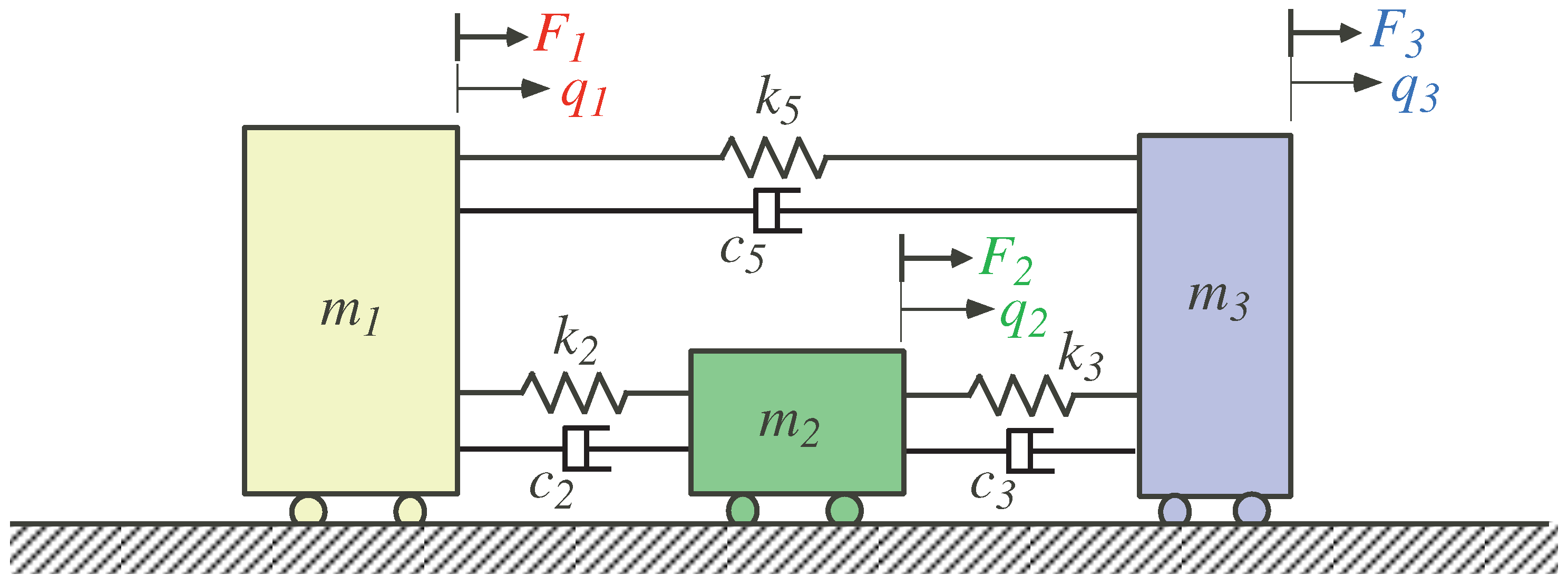
In this work, a new methodology is applied to perform a joint space analysis based on the theory of mechanical vibrations of discrete unconstrained systems. As per the expansion theorem, the solution of unconstrained systems such as the one shown in
Figure 1 can be obtained by separately solving for the rigid body and non-rigid body modes of motion; then, the linear combination of all these obtained modes form the complete response of the system. Analogous to the case of discrete systems, a closed-form solution to redundant robotic manipulators performing impedance control can be found that allows for modulating the dynamic response and selecting an appropriate set of stiffness and damping parameters according to the control criteria.
In general, in robotics there is a rule of thumb that tasks which are complex for any human being are likely straightforward for any robot, while tasks that are easy for humans end up being highly complex for any robot. Most recent advances in machine learning (ML) can successfully teach planar and general robots to perform complex tasks such as locomotion [
2,
3], and manipulation [
4,
5,
6]. Furthermore, there are ML frameworks that provide baseline algorithms [
7] which can be employed to solve general tasks. Other approaches focus these algorithms on performing industrial tasks using physical robots [
8,
9]. Meanwhile, other strategies have overcome the data hurdle by integrating ML with physical simulations [
10,
11] and employing sim-to-real techniques to transfer learned tasks from virtual to physical robots [
12].
Regarding the novel points of this work, we propose ML techniques to predict or compute the damping ratio values that correspond to the dominant oscillatory mode of motion of the multi-dimensional impedance control system of a redundant robotic manipulator. Recently, ML or deep learning techniques have been widely applied in the robotic control field, for example, in optimal impedance control for redundant manipulators (i.e., [
13]). However, in this case, the application of ML techniques for predicting the damping ratio is particularly novel. The proposed methodology differs from theory-based damping ratio calculation in that it does not require the application of mathematical equations or known physical principles in order to make estimates; instead, ML techniques use algorithms to estimate the damping ratio from historical data. A number of advantages of using ML techniques are listed below.
Improved accuracy; machine learning can analyze large amounts of historical data and learn complex patterns involving the damping ratio, thereby improving prediction accuracy.
Handling of redundant variables; machine learning is capable of handling redundant variables that can occur in a system controlled by redundant Cartesian impedance, making predictions more robust.
Ability to adapt to different conditions; machine learning algorithms can be adjusted to adapt to different operating conditions, which improves the generalization of the model.
Modal analysis data; data are obtained from modal analysis on the robot system instead of from arbitrary trial and error practices.
Continuous improvement; machine learning allows systems to improve over time, meaning that they can be updated with new data and their performance can be improved.
Use of different techniques; the use of different machine learning techniques such as XGBoost, support vector regression, random forest, LightGBM, and CatBoost allows different models to be compared and the best one applied to a given robot control system.
The rest of this article is structured as follows. In
Section 2, the current limitations on the computation of damping ratio values are described and the need for a new methodology is shown.
Section 3 states the most important basis for understanding the concept of Cartesian impedance control. In
Section 4, the dynamic response modulation of a general system with damping is described mathematically. The 3R planar robot experimental setup and data acquisition process are introduced in
Section 5. A full explanation of data preprocessing is detailed in
Section 6, along with the proposed prediction methodologies. The obtained results are presented in
Section 7. Lastly, the main conclusions are provided in
Section 8, along with possible future research directions.
2. Related Works
For general mechanical systems, the damping ratio and natural frequency are a common and appropriate set of control criteria for the dynamic response of the system. There are different methods for obtaining or computing these control criteria, among which are modelling, system identification, and automatic learning through previous data, among others that combine these principles [
14,
15]. In other applications, such as structural engineering, machine learning tools have been used to obtain equivalent damping ratios of reinforced concrete walls in seismic events [
16]. However, for redundant robotic systems performing impedance control with multidimensional mass, damping, and stiffness parameters, the computation and optimization of these control criteria, that is, the damping ratio, is not straightforward and cannot be directly treated as a decoupled system of equations, at least not from a sound fundamental point of view.
In most cases, the translational and rotational Cartesian impedance control parameters, particularly damping, are chosen in one of the following ways:. First, through trial and error on the robot setup by experimentally testing for stability regions [
17], computationally obtaining values based on previous suitable data [
18], imposing linear combinations involving the Cartesian stiffness, or arbitrarily assuming a set of
m or
n (depending on whether the equations are specified at the Cartesian or joint level, respectively) decoupled
-
-
(mass-damping-stiffness) equations (which in general is not the case) and choosing a Cartesian space damping matrix as
without considering either the effects of the off-diagonal elements of the inertia–mass matrix or performing a joint space analysis of the response using the configuration-dependant Jacobian matrix of the robot.
In order to choose or compute an appropriate set of impedance parameters, a joint space-based analysis for stiffness [
19,
20,
21] and damping makes sense, as what is physically needed to be applied is a set of joint torques at the motors of the robot within a certain desired or limited range.
For redundant robotic manipulators, where there are more joints than task coordinates
, after the Cartesian impedance system equations are mapped into the joint space those extra DoFs make the system impossible to solve analytically except by handling and solving for the rigid-body and non-rigid-body or zero-potential-energy and non-zero-potential-energy motions [
22] separately. When the system is solvable, the effect of each element of the stiffness and damping matrices can be observed and used to generate parameter studies that allow an appropriate or optimal set of values to be chosen that modulate the dynamic response according to the desired control criteria in the modal space.
3. Cartesian Impedance Control
Robotic impedance control grows out of the one-DoF second-order mechanical system with a mass, damper, spring, and external force
. When this type of system is applied to a robotic manipulator, this concept is extended to multiple DoF matrix equations with coupled non-diagonal mass, damping, and stiffness matrices with certain dynamic behavior governed by the aforementioned matrices [
23,
24]. At the Cartesian or task space level [
25], the impedance control of a robot becomes
with
being the vector of translational and rotational displacements,
the vector of external forces and moments, and the mass, damping, and stiffness matrices with subscript
C expressed in the Cartesian space. From the dynamic equation of motion of a robot provided by
where
is the vector of the
n joint angles,
M is the manipulator’s mass matrix,
G is the matrix containing the centrifugal and Coriolis terms, and
v is the gravity vector term, if we choose the motor torques
as
, the system in Equation (
2) becomes
where the external torques
and the mass, damping, and stiffness matrices establish the joint space impedance control system of equations. The respective Cartesian stiffness and damping matrices
and
can be mapped to the joint space using the manipulator Jacobian matrix
[
26,
27]
making Equations (
1) and (
3) equivalent to each other.
4. Dynamic Response Modulation of a
General System with Damping
The dynamic response of a multi-dimensional non-conservative mechanical system can be obtained in the modal space [
14], in which the multiple DoFs in Equation (
3) are decoupled such that each DoF can be independently analyzed to obtain and tune the damping ratios and natural frequencies of the response accordingly. In the case of a redundant robot performing impedance control-related tasks defined in the Cartesian space, the system in the joint space becomes positive semidefinite due to the additional (
) DoFs of the robot. This makes both the joint stiffness and damping matrices singular when they are mapped from the Cartesian space using Equations (
4) and (
5). The methodology presented here reduces the system to a positive definite system that can be solved analytically. If the robot is non-redundant, the system is positive definite and transformation to a reduced space is not necessary.
First, the stiffness and damping matrices
and
are mapped from the Cartesian to the joint space using Equations (
4) and (
5). Assuming that the external forces and changes in Jacobian are negligible, only the first term in Equation (
4) is used to map the stiffness matrix. After that, the redundancy or positive semi-definite property can be taken care of by removing the zero-potential-energy (ZP) mode of motion
using a constraint matrix
and obtaining a system in a reduced space defined as
When we remove the
r ZP mode(s) that belongs to the null space of the stiffness matrix (The ZP mode is analogous to the rigid body mode in theory of vibrations with no changes in the potential energy
of the system), Equation (
8) can be substituted into Equation (
3):
This reduced system in the
space is now positive definite and solvable for the
non-zero potential energy (NZP) modes of motion of the system by establishing the state vector
(t)=
in the state space representation:
where the
and
matrices have dimensions of
and
, respectively, and are given by
This linear system has a solution that is mainly governed by the
pairs of eigenvalues
of the
matrix, which are contained in the
matrix, which has a solution
where
and
are the right and left eigenvectors of the system. The corresponding damping ratios
in the modal space of the
matrix can be computed and systematically improved:
After the solution is obtained in the modal space, this NZP solution can be mapped back into the physical space using the constraint matrix in Equation (
8). Because the dynamic equation of impedance control of the robot can be solved analytically, the trend or behavior of the system can be obtained, as the elements of the damping matrix are iteratively changed or updated. A parameter study can be generated for all diagonal and off-diagonal elements of
, allowing the dynamic response of the system to be modulated through damping in a consistent and coherent manner.
As can be seen, this analysis in the joint space of the robot must be performed in order to modulate the dynamic response. This becomes an iterative process of determining the elements of the damping matrix that affect the most each mode of motion (vibration) as the robot moves and interacts with the environment. It is worth pointing out that, the methodology explained here can be applied in higher dimensions as well as in case of more redundant DoFs for robotic tasks; this becomes a matter of handling the redundancies by successively imposing constraint matrices () and reducing the system until it becomes positive definite.
Using machine learning tools and data collected applying the proposed methodology with modal analysis, a function that computes the optimum damping ratio can be obtained.
5. Experimental Setup and Data Collection
For a redundant robotic manipulator performing Cartesian impedance control, the analytical tool previously described is used to find an optimal damping matrix that generates the best or highest possible damping ratio of the dominant NZP (oscillatory) mode of motion having the least number of damping parameters tuned.
This work focuses on the case of a 3R planar robot, for which the set of optimal damping elements is obtained considering different paths and Cartesian stiffness matrices. Because there is no inertia reshaping, the configuration-dependent mass matrix is obtained directly at the joint space, and because for an intended task there is a Cartesian stiffness matrix associated with it, a damping matrix needs to be obtained. The were data collected for each point of a given path and then fed into the following algorithm:L.
It is worth pointing out that the damping matrix was chosen after performing the analysis described in the previous Section iteratively in order to establish a behavior and find the most suitable damping values. An experimental test consisted of finding the damping matrix elements for all the points or robot configurations in a given path. The duration of each experimental test for an intended path was 1993.74 s, with a sampling frequency of about 0.053 Hz. As a consequence, 105 samples (optimal damping values in a path) were obtained for each experiment. In other words, it takes 18.988 s to generate one sample.
Table 1 shows a description of the trials carried out for each path type in the workspace of the robot. For the circular paths, the radii values were between 0.2 and 1.15 m, for the square paths the sides lengths were between 0.3 and 1.626 m, and for the straight line paths the lengths were between 0.8 and 2 m.
To better understand the mechanics of a 3R planar robot,
Figure 2 illustrates. The motion of this robot is determined by its three revolute joints; their angular positions are described by
,
, and
. For this theoretical robot, the range of angular movement is considered to be infinite in all its joints, meaning that for any
,
.
In this way, the revolute joints do not impose any restriction on the robot’s workspace. On the other hand, the link lengths restrict the robot’s reach. This study considers m, m, and m, with corresponding link masses of kg, kg, and kg.
Because a redundant 3R planar robot is being considered, the number of joint space variables should be greater than the number of controlled task space variables. In
Figure 2,
are the three joint space variables and
,
, and
are the task space variables. No access to control
is assumed in order to impose redundancy on the model. This means that the size of the manipulator Jacobian is 2 × 3. Consequently, the mapping from the Cartesian to the joint space provides a positive semi-definite system with singular
and
matrices, which is not solvable unless the system is reduced to a positive definite one using the methodology previously described in this paper.
Local Optimum Damping Based on Modal Analysis
Before extending to a path, it is necessary to explain how to obtain the optimal damping values for a given point or joint configuration, after which generalizing it for paths is a matter of applying the algorithm to all the points that are part of the pre-established path.
Figure 3 describes the process of obtaining an optimum damping value for a configuration of a redundant 3R planar robot. For greater comprehension, we explain this by an example in which the end effector is located at
m,
m]
.
The input data are provided by the joint configuration vector
, which corresponds to the Cartesian
, the inertia mass matrix
, a desired stiffness matrix in the Cartesian space
, and the configuration-dependent Jacobian matrix of the robot
. All of these data except for the Cartesian stiffness matrix depend on the current robot configuration. The joint configuration vector is obtained by applying inverse kinematics to
,
= [
,
,
]
=
rad. Considering this configuration,
Then, mapping the Cartesian stiffness matrix to the joint space using Equation (
4) and assuming negligible changes in Jacobian, the joint stiffness matrix
is obtained:
As expected from theory, due to the redundancy this joint stiffness matrix is positive semi-definite. In order to remove the ZP mode, a state vector in the null space of
must be found and normalized with respect to
such that
. For this illustrative example, the normalized vector is
When the constraint matrix
is imposed to the system such that
, the redundancies are removed. This means that
and
are reduced to
and
through Equations (
8)–(
10):
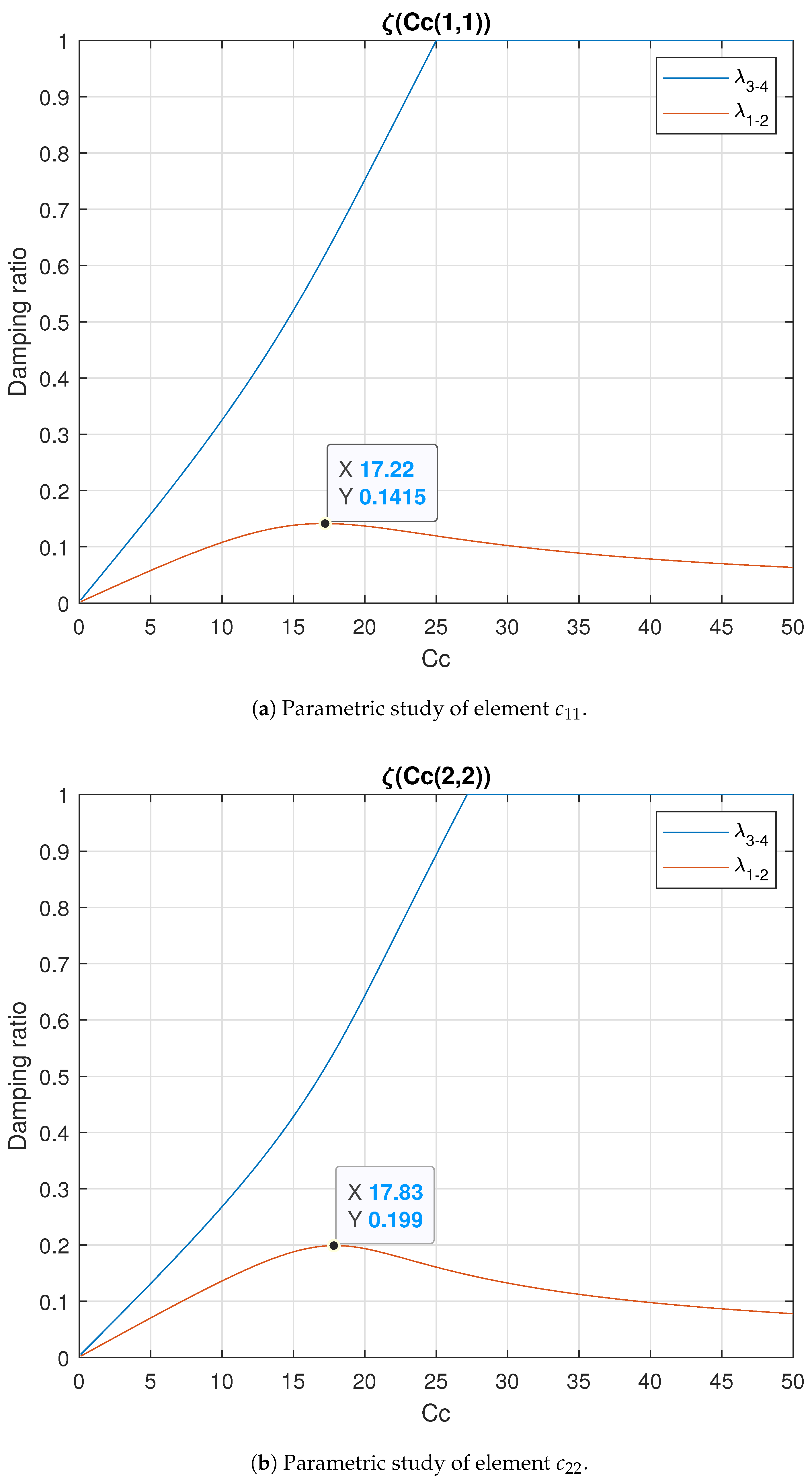
From this point on, a parametric study is carried out with the purpose of analyzing the influence of the damping matrix on the damping ratios of the system. The damping ratios affect the dynamic response of the robot under impedance control, and are very important. To accomplish this parameter study, one element from the main diagonal of the damping matrix is iteratively increased while the other one remains with a low value (0.1 ) in order to obtain the effect of the element in study over the damping ratios. Please note that it is important to maintain the positive definite property of the damping matrix. A step of 0.001 was used for the iterations, beginning with a = diag(0.1, 0.1) for the first iteration (j = 1) in both parametric studies. Note that for the first iterations, the results of both parameterizations are very alike, as the values are very low.
For both the and parametric studies, the iteration j = 40,000 is shown as an example in order to clarify the procedure.
For the first parametric study (
), we have
Mapping the Cartesian damping matrix onto the joint space with the help of Equation (
5), we have
Reducing C, we have
The next step is to obtain the system matrix (
) from the space state representation, as described in Equation (
12):
To obtain the damping ratios, the eigenvalues of the
matrix are needed, and can be obtained using the equations in (
14):
For the second parametric study (element
), the same procedure is followed:
For the complete parametric study at this robot configuration, 49,901 iterations have been considered; the whole analysis results are illustrated in
Figure 4.
From observation and experimentation, it became understood that the most critical mode is
, as it is not significantly influenced by any of the elements of the damping matrix. The element with the greatest influence on mode 1-2, comparing
Figure 4a,b, is
, and the higher damping ratio values for this mode were obtained with the variation of this element. Because the damping ratios for mode 1-2 have a unique maximum, the optimum values for the elements of the damping matrix can be chosen.
Thus, for this configuration, the optimum damping matrix is
Leading to the following damping ratios:
This analysis for one robot configuration corresponding to a point in the intended path is then extended for each configuration along the path.
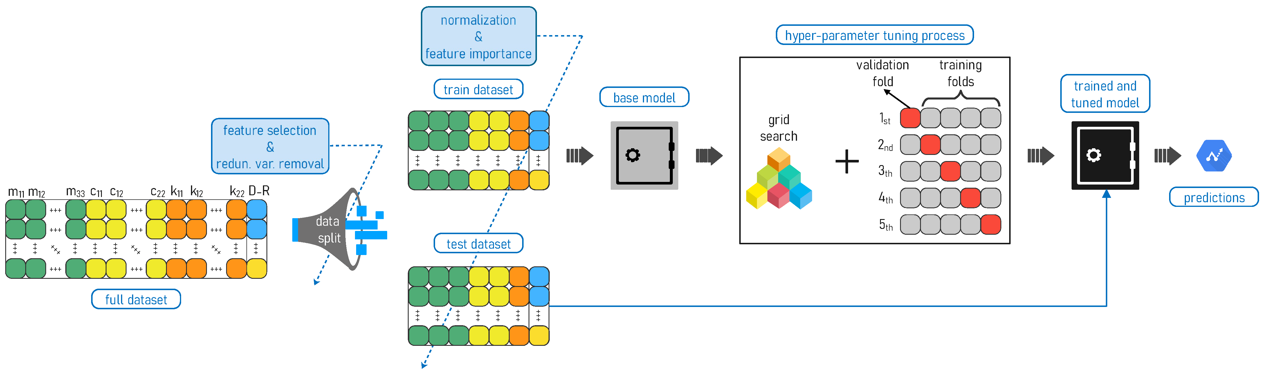
6. Methodology
In the creation of data-driven machine learning models, the adage “garbage in, garbage out” is applicable [
28]. In actuality, real-world data are frequently erroneous and deficient in specific behaviors or patterns, and are frequently inconsistent and incomplete. Data preprocessing is therefore essential for overcoming the aforementioned problems and for preparing the data to create data models [
29]. Data cleansing, normalization, feature discovery (i.e., feature extraction, feature selection, and feature learning), and unbalanced data management are often included in data preprocessing activities.
In this section, all the steps used to preprocess the data are described, including splitting of the data into training, validation, and testing sets as well as several preliminary considerations regarding the data, feature selection and redundant variable removal, and data normalization using scaling strategies.
Then, the basis of the five proposed ML algorithms are addressed. Likewise, the details of the ML algorithm-based architectures are described. Finally, the technique employed for hyperparameter tuning (grid search plus CV) is outlined.
6.1. Data Split
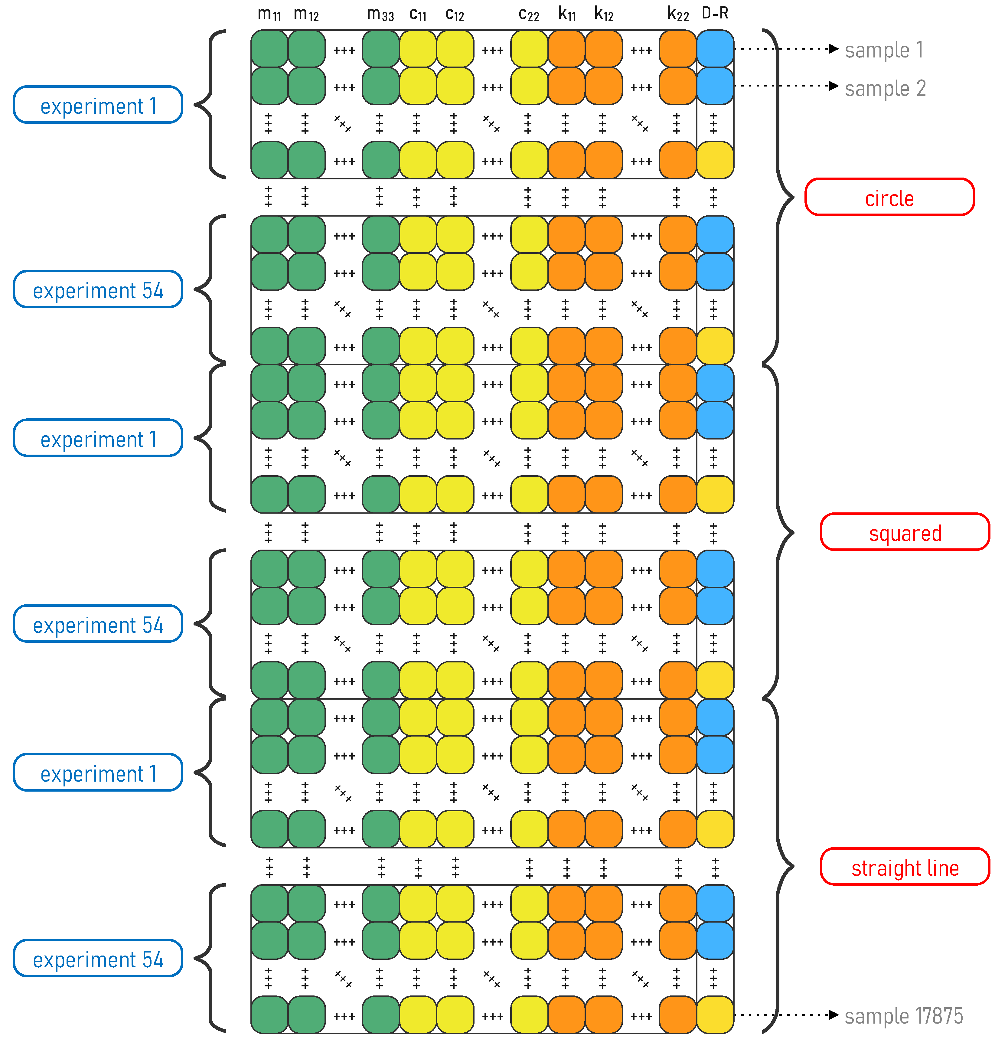
Typically, the full dataset (see
Figure 5) can be divided into two or more subsets, i.e., for training, validation, and testing. Training and testing datasets are the most common in ML models; however, a validation dataset is frequently required as well. Training sets are usually employed to estimate the parameters of the model and fit the data. After that, a test set is used to evaluate the model and measure its performance. When a third set is used (validation), it is commonly intended to change or calibrate the hyperparameters of the model. If only the training and testing sets are used, another strategy, such as cross-validation (CV), can be applied to calibrate the model, and a third dataset is not required. In this work, only two datasets, training and testing, are used. Moreover, during testing a CV strategy is applied to calibrate the model.
There is no fixed guideline for splitting data. There are several strategies to perform the task, such as random sampling, stratified random sampling, or non-random sampling. Considering that our experiments are classified into three path types (square, straight line, and circle) it is important to ensure that the data are balanced (correctly distributed) with respect to those paths in the training and testing sets; thus, stratified random sampling is suitable.
From
Table 1, the number of total samples for each path can be observed. Each path in the dataset is split into 80% for training and 20% for testing. Next,
Table 2 shows the total samples corresponding to each dataset (training and testing). Taking the total samples for training (14,299) and testing (3576) and dividing by the total samples (17875), it can be confirmed that the total distribution is 80% and 20%, respectively, as expected.
6.2. Preliminary Considerations
Based on
Section 5, the input data are composed of the predictor variables (elements of matrices M, K, and C) and the target (damping-ratio). Regarding the predictors, as they are elements of matrices there are several considerations to be taken into account. For instance, the K matrix is joint-form, which implies that it is a diagonal matrix. Thus, all the entries outside the main diagonal (drawn from left to right) are zero, i.e., the elements
and
. A similar case is the C matrix; as it is a diagonal matrix, its elements
and
are zero. In consequence, as those four elements are always zero they do not provide useful information to the input data, and must be removed.
To ensure that the rest of features (elements of matrices) can provide useful information to the input data, the standard deviation was computed for each feature in order to measure how many features vary (a measure of variance) throughout the dataset. If a feature does not vary, it is unnecessary and should be removed. Below,
Table 3 shows the standard deviation computed on the predictors.
From
Table 3 it can be seen that the elements from matrices
and
have quite a significant deviation, unlike matrix
, in which there are elements with low but still significant deviation (i.e., with at least two significant decimal values). However, the element
has a standard deviation equal to 1.994 × 10
−14, which is completely negligible. This element must be removed, as it does not vary at all throughout the dataset.
In summary, with these preliminary considerations several elements of the matrices have been removed. The remaining eleven parameters include eight for , two for , and one for .
6.3. Feature Selection
The process of choosing a subset of pertinent features to be used in model creation is known as feature selection, or sometimes as variable selection or attribute selection. Feature selection is usually carried out for several purposes. First, it can enhance a machine-learning algorithm’s performance [
28]. For instance, certain features could be noise, or may not be important for a specific problem. These features contribute to overfitting, which can lead to biased or undesirable variation in the problem result. Second, feature selection is carried out to increase the model’s interpretability [
28]. The model is made simpler when certain features are eliminated. In order to better understand which features contribute the most to the model, feature selection additionally rates the relevance of the features. Third, feature selection lowers the amount of resources needed for computation and data collection [
28]. For instance, if sensor data are utilized as features, feature selection aids in reducing the number of sensors, lowering the cost of the sensor system, as well as the costs associated with data gathering, storage, and processing. Finally, feature selection works to lessen the possibility of the “curse of dimensionality,” similar to dimensionality reduction.
In this work, considering that the full dataset contains several experiments and each is performed under different execution conditions, there is not any guarantee that the predictor variables have a linear relationship, either between themselves or with the predicted or target variables. Under this scenario, a linear measure of correlation such as the Pearson correlation is not appropriate; instead, other techniques for measuring correlation that are able to capture nonlinear relationships should be employed, such as Spearman’s rank correlation, distance correlation (DC), mutual information (MI), ANOVA f-test, Chi-square test, and variance checking, among others. In this work, three different methods, Spearman, MI, and DC, are used to measure the feature–target (feature selection) and feature–feature (redundant variables removal) correlation. Each method and its details are explained below.
6.3.1. Spearman’s Rank Correlation
Known as Spearman’s rho, this is a non-parametric measure of the association between two variables. In the context of this study, it can be used to measure the correlation between different features of the robot, such as its control parameters and damping ratio.
As is well known, Spearman’s correlation varies in a range from
to
, where
is associated with the maximum negative relationship between two variables and
represents the maximum positive one [
30]. Based on [
31], an absolute correlation coefficients between
and
represents a negligible correlation, i.e., those predictor variables should be removed.
Figure 6a shows the Spearman correlation matrix among the predictor variables and with respect to the variable to be predicted.
The last row (from top to bottom) contains the correlation coefficients between the predictor variables and the target (feature–target). It can be seen that these coefficients vary in a range of
to
(moderate, weak, and negligible correlations). In this sense, as there are no higher coefficients and not very many predictor variables, it is not suitable to remove them. Therefore, in
Section 6.4 all of the features are evaluated in order to eliminate those that are redundant.
6.3.2. MI Correlation
MI is a concept used in feature selection that measures the dependence between two variables [
32,
33]. In this work, MI can be used to measure the dependence between the input features of the robot, such as its control parameters, and the output feature, such as the damping ratio. The MI between two variables is a non-negative value, with larger values indicating stronger dependence between the variables.
Figure 6b shows the feature–feature and feature–target MI correlation matrix. As mentioned above, the last row from top to bottom contains the correlation coefficients between the features and the target. After observing these values, the variables with coefficients closer to 0 are eliminated, considering a cut-off value of 1.5; Considering this, the remained features are
,
,
,
,
,
,
, and
. This means that, in
Section 6.4, those features are evaluated to determine which are redundant and should be removed.
6.3.3. DC
DC is a statistical measure that quantifies the dependence between two random variables. In feature selection, it can be used to measure the dependence between the input features and output feature of a model [
34]. DC has the advantage of being able to detect nonlinear relationships between variables, making it a useful tool for feature selection in situations where the relationships between features and the output are nonlinear [
35].
The DC coefficient is a value between 0 and 1, where 0 indicates no dependence between the variables and 1 indicates perfect dependence. The coefficient is calculated as the square root of the ratio of the distance covariance and the product of the distance variances of the two variables.
Figure 6c shows the feature–feature and feature–target DC matrix. As in the previous cases, the values of the last row from top to bottom correspond to the feature–target correlation coefficients. Values between
and
represent a negligible correlation, i.e., those features should be removed. Considering this, the remaining features are
,
,
,
,
,
,
, and
. In
Section 6.4, these features are evaluated to determine which are redundant and should be removed.
6.4. Redundant Variables Removal
Accuracy and elapsed time are two crucial factors to be considered when ML models are built, as it is desirable for the model to have excellent performance, i.e., the best accuracy and the least elapsed time for the training and testing stages. Feature quality is a key point to achieve this, as redundant variables (two or more predictors that explain the same information) result in poor model performance [
36].
Regarding the Spearman and DC correlation, when the absolute correlation coefficient fluctuates from 0.90 to 1.00 it can be considered as a very strong correlation [
31]; thus, if two predictor variables have a very strong correlation one of those must be removed to avoid redundant features. On the other hand, concerning MI correlation, if the correlation coefficients are less than 1.50 (cut-off value) it means that those variables are sufficiently independent of each other.
Table 4 summarizes the feature selection and redundant variables removal process carried out to select the predictor variables used in the next stage of the methodology. The “Feature Selection” column summarizes the discussion about the correlation of all the features against the target in order to determine which should be kept or removed. Thus, in this part, only the features that contain a (
✓) are assessed in the next column, “Redundancy Analysis”, to determine whether they are redundant with another feature, while those that contain a (
✗) symbol are excluded from the next analysis, as they are not strongly correlated with the target.
The column “Redundancy Analysis” recaps what was discussed in the previous paragraph about two features being considered redundant or not. Based on that, the (✓) symbol determines the non-redundant features that are kept, while the (✗) symbol points out the features that are redundant and should be removed; (***) indicates features that were not evaluated because they were excluded in the previous feature selection phase.
Finally, as three methods are selected to perform redundant analysis, a feature is kept only if all three, or at least two, provide a (✓) symbol to the feature; otherwise, it is not considered for integrating the predictor set and receives a (✗) symbol.
Therefore, after this thorough feature selection process, the remaining features from the initial dataset are
6.5. Data Normalization
Predictors can come from different data sources, which can have varying order of magnitude. To accelerate training or improve a model’s generalization capability, a data scaling strategy can be applied [
37]. There are several normalization or standardization techniques, including Min-Max, Stardard, Robust, and L1, among others [
29]. Based on our experiments’ nature (simulation), there are no outliers; thus, the Min-Max technique is applied, considering that this strategy is usually weak to the presence of outliers. Min-Max scales data in the
range using a linear transformation based on the original data range. Thus, through this process it is ensured that data are scaled to the same proportions and in the same range for all features.
Next, as indicated at the beginning of this section, it is essential to recall the foundations of the proposed ML techniques as well as the details of their algorithm-based architectures.
6.6. XGBoost: eXtreme Gradient Boosting
This algorithm, which is applicable to both regression and classification, was first developed by Chen et al. [
38]. It is an ensemble in which boosting properties are leveraged by aggregating new models to adjust errors in the performance of the existing models. This task is recursive until no noticeable improvements are detected, then the task stops. When boosting is combined with a gradient basis, the new models that are added can help to predict the residuals or errors of prior models. Finally, the models aggregated to make a final prediction. During this step, a gradient descent algorithm is employed to minimize the loss when new models are added. Notably, XGBoost won on 17 of the 29 machine learning tasks launched by Kaggle by 2015.
As with many other machine learning algorithms, XGBoost requires a careful tuning process to determine the optimal performance. Moreover, this algorithm has several hyperparameters that need to be tuned; for that reason, the tuning process needs to be performed appropriately. Strategies such as Grid Search can be used to search for optimum hyperparameter combinations.
6.7. RF: Random Forest
An RF is an ensemble of decision trees used to forecast the output from a set of predictors [
39]. On a training dataset, decision trees are built to obtain the prediction results in either mode (in case of classification issues) or the mean prediction (in case of regression issues) of the individual trees [
40]. During the training stage, a bootstrap sample function is employed to randomly split the dataset into homogeneous subsets. While a random subset is used to train each decision tree, the rest of the subsets are taken to validate the tree and compute the model accuracy [
40,
41]. Moreover, similar to XGBoost, this algorithm requires tuning of the hyperparameters to achieve its best performance.
6.8. LightGBM
This is an open-source gradient-boosting framework that uses tree-based learning algorithms. It is designed to handle large-scale data and has been widely used in various applications, such as recommendation systems, click-through rate prediction, and machine learning competitions. LightGBM is particularly efficient at handling large datasets and high-dimensional data, as it uses a histogram-based algorithm to split the tree leaves, which reduces the complexity of the model and speeds up the training process [
42].
Compared to XGBoost, while both are powerful gradient-boosting libraries that have been used in many machine learning tasks with good performance, LightGBM is generally faster, more memory efficient, and is better able to handle categorical features and missing values, making it more suitable for large-scale data.
6.9. CatBoost
This algorithm can be used for both classification and regression tasks. For regression problems, it uses a different loss function, such as mean squared error or mean absolute error, to optimize the model. It permits using other loss functions as well [
43]. CatBoost is particularly suitable for datasets with a large number of categorical features and missing values, as it has built-in handling for both.
Compared to RF, CatBoost is generally more powerful and accurate for regression; however, it can be more complex and require more computational resources. Compared to XGBoost and LightGBM, CatBoost has better ability to handle categorical features and missing values, which can be beneficial when working with datasets with a high number of categorical features.
6.10. SVR: Support Vector Regressor
Support vector machine is a well-known ML algorithm to deal with data classification challenges where high-dimensional data and small training datasets are not an issue. However, computational resource demands can reach high levels if caution is not taken [
44]. This algorithm is extremely well equipped to deal with regression issues.
6.11. Hyperparameter Tuning Process for Models
The hyperparameter tuning process can be performed on a grid or by random search. Random searching (non-discrete or parametric values) tends to consume a higher level of computational resources than grid search; thus, in this study we have employed grid search. In grid search, reasonable ranges (parametric values) must be initially proposed as the hyperparameter combinations are set and tested on this basis.
On the other hand, K-fold cross-validation is used to assess model performance during the tuning process, with cross-validation adopted as a strategy to avoid overfitting. For this work, is taken as a popular fold-division number, i.e., the data are divided in five folds. Four-fold validation is typically intended for training, with the remaining data used for validation. After that, the data used for validation pass through to become part of the training folds, while one of the four folds initially used for training passes through to become the new validation fold. This iterative task executes until all folds have been used for validation. When this process is complete, the data are reshuffled and cross-validation is repeated; for our case, three repetitions were set.
The five proposed models each have several distinct hyperparameters that need to be tuned.
Table 5 presents the most popular hyperparameters for each model and defines the parametric values used for cross-validation.
6.12. Feature Importance
This process refers to the relative importance of different features in a dataset for a given model. It is a measure of the impact that each feature has on the model’s predictions. There are a variety of feature importance measures, such as the permutation-based importance (PbI), mean decrease impurity (MDI), and mean decrease accuracy (MDA), that can be used to determine the importance of each feature. Both this method and feature selection are important steps in the process of building machine learning models, and can help to both improve the performance of the model and to understand the relationships between the features and the output.
In this study, the MDI (or Gini importance) [
45,
46] and PbI [
47] are used to perform this task. On the one hand, the Gini importance looks at how a random forest is constructed and measures how each feature decreases the impurity of the split; the feature with the highest decrease is selected for the internal node. For each feature, it can describe the average decrease in the impurity. The average over all the trees in the forest is the measure of the feature importance. On the other hand, PbI, apart from analyzing feature importance, is employed to overcome the drawbacks of default feature importance computed with MDI. PbI randomly shuffles each feature and computes the change in the model’s performance. The features which impact the performance the most are the most essential ones.
In this work, RF is the algorithm employed to determine feature importance, following training and tuning using a five-variable predictor set. Note that after choosing the features with the highest impact for the RF model, it should be re-trained and re-tuned for predicting damping ratios. The other models are trained only once, and perform the prediction using the most important features.
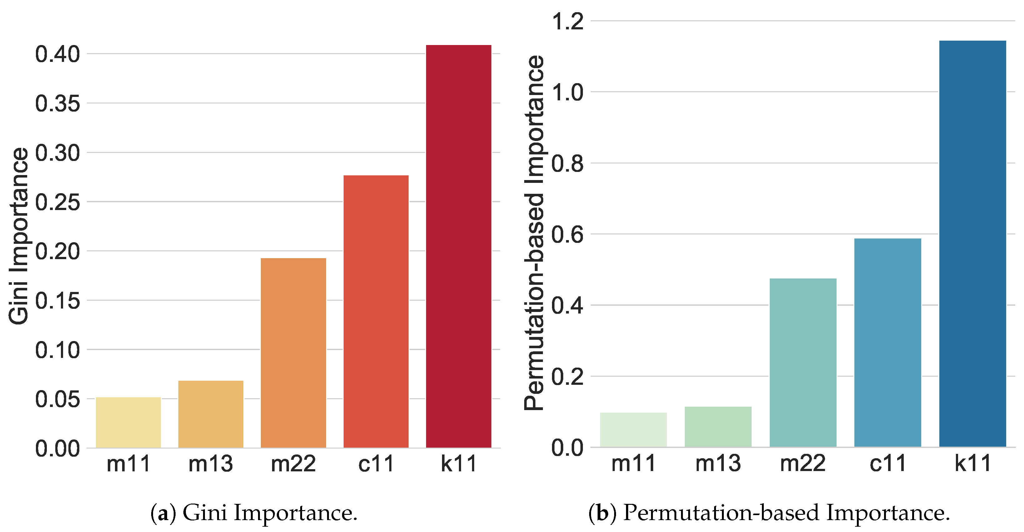
Figure 7 shows the feature importance analysis using the two above-mentioned methods, MDI and PbI. Gini importance analysis (see
Figure 7a) performed over the variables, as mentioned in
Section 6.4, clearly shows that
and
are the features with the least impact on the model, and should be removed. This idea is supported by PbI analysis (see
Figure 7b), where the same two variables have the least impact on the model. In conclusion, the predictor set is finally reduced to three variables:
,
, and
.
As a final point,
Figure 8 shows the flow of the entire applied methodology and summarizes all the steps described in
Section 6.
7. Results and Discussion
Through K-fold cross-validation, each one of the five stated algorithms was trained and validated to obtain the best possible combination of hyperparameters allowing for the highest accuracy (
score) in predictions for optimum damping ratios. Thus,
Table 6 shows the most suitable hyperparameters that could be found for the LightGBM, CatBoost, XGBoost, SVR, and RF models.
With the chosen hyperparameters, each model was retrained and retested. At this point, it should be noted that one-way testing was usually performed, with no splitting or cross-validation. When evaluating model performance on the test dataset, the model may suffer from overfitting to the test data. Using cross-validation, the model’s performance is estimated on different subsets of the data, leading to a more unbiased estimate of the model’s performance. Furthermore, cross-validation provides a more reliable estimate of the model’s performance by averaging the performance over multiple subsets of the data. This is especially useful when the sample size is small or the data are unbalanced, in which case a single training–testing split may not be representative of the model’s performance. In this work, testing is carried out using cross-validation.
Classic model assessment characteristics to measure performance are the training and testing time, an error metric such as the root mean square error or RMSE, and the training and testing accuracy (
score).
Table 7 shows these characteristics in order to assess and discuss the models’ performance.
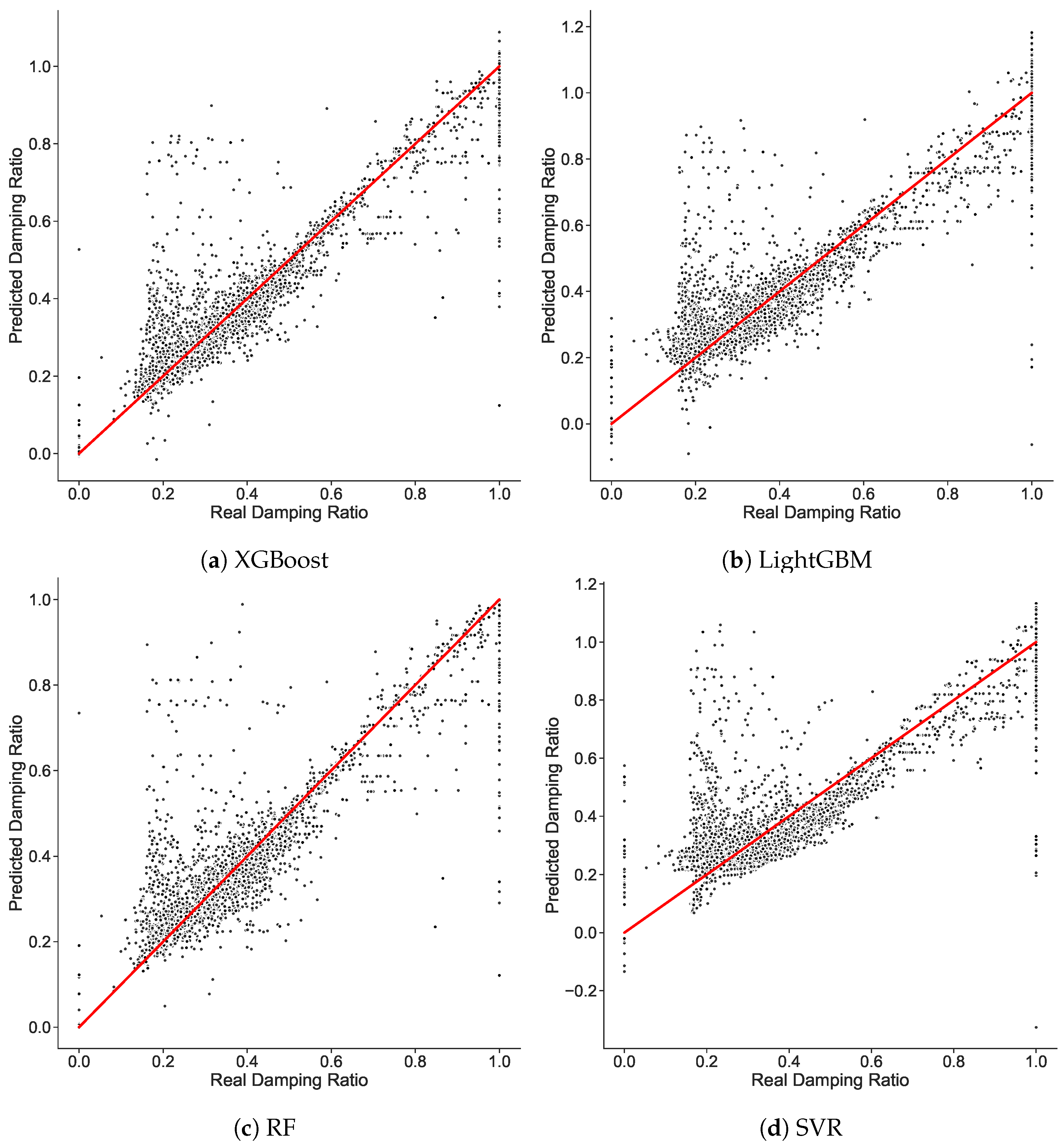
Comparing the five models, it is noticeable that both the XGBoost and RF models have the highest average accuracy in the tests (86.27% and 83.11%, respectively), and outperform the LightGBM, SVR, and CatBoost models. During training, the average accuracy of XGBoost is quite similar to that of RF. In terms of RMSE, XGBoost has the lowest value in testing. Thus far, considering these characteristics, XGBoost has the best performance. However, in terms of the elapsed time needed to train or test a model, LightGBM is much faster than XGBoost. This is a great advantage if a model is intended to be deployed into production, as in the ML lifecycle the control time is quite critical.
As can be seen, CatBoost performs poorly, reaching an average accuracy of 20.50% in testing and19.75% in training. The reasons for this could be due to a number of aspects. On the one hand, this model is probably too complex for the given dataset, memorizing the training data instead of generalizing to new data. Another possibility is that the model is too simple for the given dataset, and is not able to capture the underlying patterns in the data.
It is always important to visualize the results in graphics; as such,
Figure 9 shows the scatter plots for the different tested models, with real datapoints plotted against the predicted values. Following this idea, it is expected that better prediction will result in datapoints being plotted closer to the straight curve, with a slope equal to 1. The XGBoost model meets almost all the conditions to be the model with the highest performance, followed by the RF model, then the LighGBM model, and finally the SVR model. In terms of accuracy, the XGBoost and RF models have almost the same percentage;
Figure 9a,c shows that most of datapoints are nearer to the straight curve. However,
Figure 9d shows that many datapoints are far from the straight curve, indicating the low accuracy and performance of the model. It should be noted that the scatter plot figure for the CatBoost model is not shown due to its very poor performance.
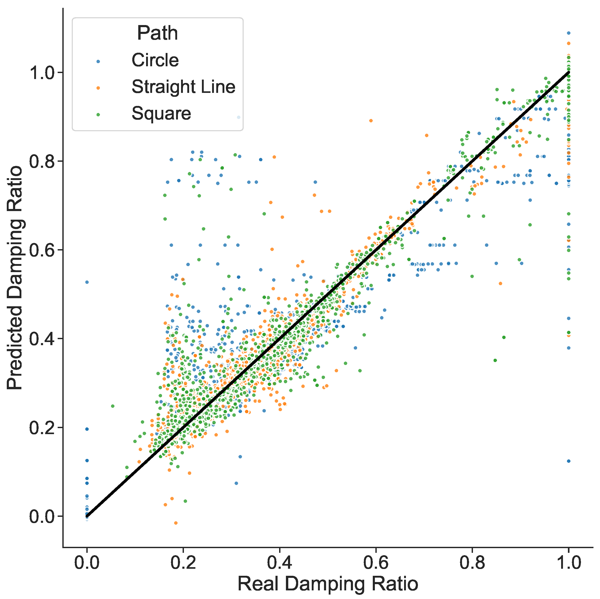
On the other hand, recalling that the dataset was built with simulations of three different path types, it is important to analyze how the prediction of the data points associated with each path perform. Based on this, the XGBoost model has the best performance,
Figure 10 highlights the location distribution of the datapoints associated with each different path type.
Considering each path, it is possible to observe the trend of the prediction results. Essentially, the straight line and square paths have the best predictions performance, while the circle has a larger error. This behavior is corroborated by
Figure 10, where the furthest data points of the trend line are the blue ones that belong to the circle path, while the nearest ones belong to the other available paths.
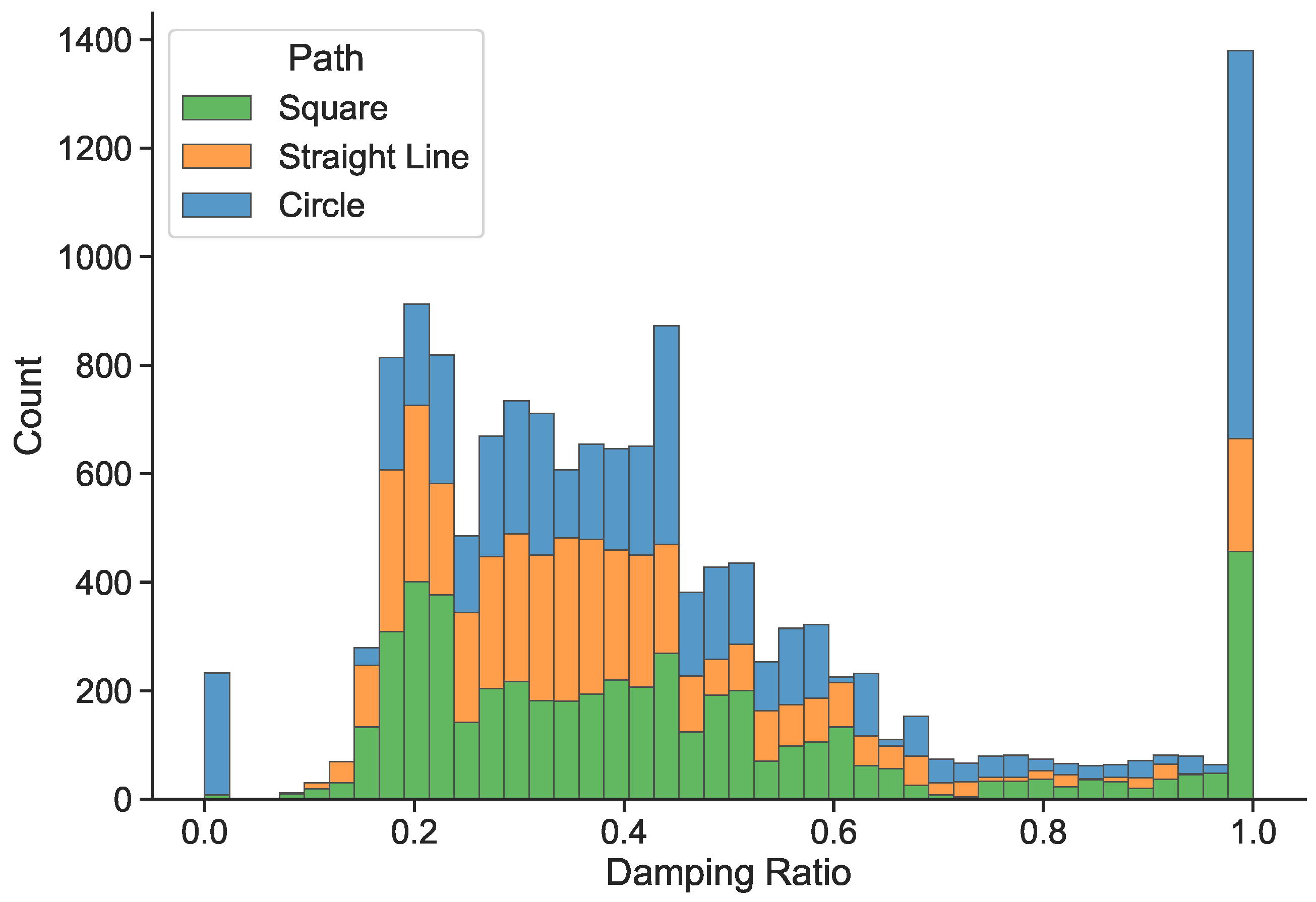
In addition, as can be seen in
Figure 10, there are outliers at the extreme real damping ratio equal to one. This shows that the model is better at predicting certain damping ratio values than others. For this reason, we decided to carry out an analysis of sample frequency distribution for each value of the damping ratio in the training dataset. Despite the fact that, as shown in
Table 2, the dataset is relatively balanced in terms of the number of samples for each type of trajectory, it can be seen in
Figure 11 that this is not the case for the number of samples for each value of the damping ratio.
It should be remembered that data preprocessing (feature selection and redundant variables removal) was carried out considering this imbalance of samples in terms of damping ratio values. This could have led to the elimination of variables that would have helped the model to predict whether they correspond to one damping ratio or another. For this reason, as mentioned in the next section, in future work it is important to ensure a balanced dataset in terms of the number of samples per value of the damping factor.
8. Conclusions and Future Work
This study has shown, as expected, that different configurations of a robotic manipulator result in different dynamic responses as the robot moves along a given path. To maintain a dynamic response as close as possible to the desired level, joint space analysis with corresponding damping value updates must be performed and implemented. A parameter study based on the modal analysis and optimization for damping ratio values is computationally expensive, especially when the robot includes more DoFs or task coordinates that need to be analyzed.
This study proposes and validates an innovative and advanced damping factor prediction method. Specifically, instead of using the seventeen variables that normally make up the matrices, the five ML models tested here only need one value from the matrix (), one value from the matrix (), and one value from the matrix (), providing a total of only three variables. Furthermore, the stated strategy works under the different path types (circle, square, and straight line) to which the 3R planar robot is subject.
The three main contributions of this work are: (i) preprocessing (data cleaning, normalization, feature importance, and rendundant variables removal) of the variables from the matrices derived from various time and experiments; (ii) selection of the best model hyperparameters based on the grid search technique; and (iii) the training and testing of five different ML models using K-fold cross-validation. Furthermore, the K-fold cross-validation strategy utilized in the proposed method eliminates the need for a validation dataset. The developed damping ratio prediction approaches with the best hyperparameters work very well, with accuracy ( score) results higher than 86% and RMSE outcomes less than 0.094. With the XGBoost and RF models in particular, a significant overall accuracy greater than 83.1% is attained. The XGBoost model achieves an inference time on the test data of 0.05 s, making it extremely adaptable to real-world scenarios. Comparing the test time with the time required to generate a sample (18.99 s), sample generation is 380 times slower than the ML model. These findings demonstrate the potential of ML models for the creation of robot damping prediction systems.
It is important to clarify that there are several limitations and considerations that can affect the performance of machine learning algorithms used for damping ratio prediction, among which are the following:
Data quality: machine learning algorithms require a large dataset to train and validate the model, and their performance can suffer if the data are incomplete, noisy, or irrelevant.
Model choice: Tte performance of machine learning algorithms can depend on model choice, and it may be necessary to try several different models in order to find the best fit for a particular problem.
Overfitting: machine learning algorithms can overfit the model to the training data, which can reduce the model’s accuracy on new data.
Generalization: machine learning algorithms may not generalize well to new data if not enough training data have been used or if all relevant variables have not been considered.
As future work, we intend to extend the present analysis for prediction of optimal damping ratios in real robot applications in addition to simulated robots. An important point is to generate a balanced dataset in terms of the number of examples per type of trajectory, as well as the number of samples for each value of the damping ratio. Furthermore, it is desirable to expand the methodology to higher-dimensional and highly redundant systems, as this can be an excellent tool for system identification and modulation of dynamic response.


 ,
, 


