Optimal Designs for Antoine’s Equation: Compound Criteria and Multi-Objective Designs via Genetic Algorithms

Abstract

Antoine’s Equation is commonly used to explain the relationship between vapour pressure and temperature for substances of industrial interest. This paper sets out a combined strategy to obtain optimal designs for the Antoine Equation for D- and I-optimisation criteria and different variance structures for the response. Optimal designs strongly depend not only on the criterion but also on the response’s variance, and their efficiency can be strongly affected by a lack of foresight in this selection. Our approach determines compound and multi-objective designs for both criteria and variance structures using a genetic algorithm. This strategy provides a backup for the experimenter providing high efficiencies under both assumptions and for both criteria. One of the conclusions of this work is that the differences produced by using the compound design strategy versus the multi-objective one are very small.

1. Introduction

Antoine’s Equation is a class of semi-empirical equations that represent the non-linear thermodynamic relationship between equilibrium vapour pressure, P, and temperature, T [1]. The equation is $P\left(T\right)={10}^{a-\frac{b}{c+T}}+\epsilon$, and it was developed and introduced in 1888 by Louis Charles Antoine. The unknown parameters of the model (a, b, c) are numerical constants related to the enthalpy and entropy of vaporisation. Usually, Antoine’s Equation cannot be used to describe the entire saturated vapour pressure curve because it is not flexible enough. Therefore, multiple parameter sets are commonly used for a single substance. A low-pressure parameter set is used to describe the vapour pressure curve up to the normal boiling point, and the second set of parameters is used for the range from the normal boiling point to the critical point.

Vapour pressure has a wide range of industrial applications [2], such as the handling of liquids and gases [3], distillation processes to separate chemical substances, such as bio-diesel production [4], operation of aerosols and atmospheric modelling [5], safety and performance specifications of fuels [6], engineering production like solar cells [7], etc.

Let us define ${\theta }^t=(a,b,c)$ as the unknown parameter vector. Since the Antoine Equation is non-linear for the parameters, local optimisation will be considered, for which a set of nominal values or best guesses of the unknown parameters, ${\theta }^{\left(0\right)}$ will be needed [8]. The design will not depend on a since ${10}^a$ is a linear factor of the model [9].

It is common in statistical modelling, and particularly in optimal experimental design, to assume the variance of the response to be normal homoscedastic. A normal homoscedastic response corresponds with a constant absolute error. However, in [10], it is suggested that the response is indeed normal, but the relative error is, in fact, constant. This is equivalent to considering a particular normal heteroscedastic variance of the response. Single objective designs for each of these are calculated and compared in [11]. In the heteroscedastic model, the dependence of the variance on the explanatory variable is expressed by the so-called weight function, $\lambda \left(T\right)$ [12]. Its value comes from $Var\left(P\left(T\right)\right)={\lambda }^{-1}\left(T\right){\sigma }^2$, with $\lambda \left(T\right)=1$ for the homoscedastic case and $\lambda \left(T\right)=1/\eta {\left(T\right)}^2$ for the heteroscedastic case. The models for the homoscedastic case are

$$P_o\left(T\right)={\eta }_o\left(T\right)+\epsilon ={10}^{a-\frac{b}{c+T}}+\epsilon ,\epsilon \sim \mathcal{N}(0,{\sigma }_o^2),$$

(1)

and for the heteroscedastic case

$$P_e\left(T\right)={\eta }_e\left(T\right)+\epsilon ={10}^{a-\frac{b}{c+T}}+\epsilon ,\epsilon \sim \mathcal{N}(0,{\sigma }_e^2{\eta }_e{\left(T\right)}^2).$$

(2)

where ${\sigma }_o$ is the standard deviation of the response for the homoscedastic case, and ${\sigma }_e$ is the squared value of the relative error when this is constant, the heteroscedastic case.

Given the ambivalence with respect to the variance structure, special considerations are required when working statistically with this model or any other with uncertainty in the probability distribution. Throughout this paper, the implications will be highlighted, and different methodologies will be proposed to deal with this question from an optimal experimental design perspective.

Contributions, Objectives and Organisation

Optimal experimental design is an interesting field for the application of optimisation algorithms. In this work, we provide an implementation of the genetic algorithm adapted to approximate designs in the context of optimal experimental design, in particular, the insufficiently explored use of a multiobjective metaheuristic. With this tool, the issue of the probability distribution for Antoine’s Equation is tackled for different optimality criteria. Along with the solution provided, an initial comparison of the typical methods of optimal experimental design, compound criteria, with the metaheuristic multiobjective algorithm is given. The genetic algorithm is more flexible in adapting to other models, criteria or a number of objective functions and scalable to a larger parameter size and a number of independent variables.

The aims of the study are three. First, to provide the practitioner with optimal designs that take into account the probability distribution of the response variable, as it drastically affects the efficiency of optimal designs for the problem, providing efficient solutions for either of these alternatives for different optimality criteria. Second, to explore the differences, or lack thereof, of the solutions provided by the stochastic results of a multiobjective metaheuristic versus several iterations of a compound algorithm. Finally, to highlight the potential value and flexibility of this family of algorithms in the design of experiments field.

The article is structured as follows: Section 2 provides context and theory about optimal experimental design theory and its application to Antoine’s Equation; Section 3 summarises the methodologies applied to address the issues raised in this article by the different interests of the experimenter; in Section 4 the proposed algorithm is described in detail; Section 5 includes the performance and main results of the implemented algorithms, and Section 6 summarises the main points and implications of this paper.

2. Background

This Section gives an overview of the optimal experimental design theory covered by this article as applied to Antoine’s Equation. A summary of the optimal designs and their efficiencies when different optimality criteria or variance structures are considered is also provided.

2.1. Optimal Experimental Design Theory

Optimal experimental design (OED) aims to find the best points at which to perform an experiment. In the theory of optimal designs, the baseline is a model or set of regression models, which can be denoted by

$$y=\eta (T,\theta )+\epsilon$$

(3)

where $\eta (T,\theta )$ is a function of $\theta$, the vector of unknown parameters of the model, y is the response variable, $T\in \mathcal{X}$ is the independent variable, with $\mathcal{X}$ being the design space and $\epsilon$ the random error, following a probability distribution, usually a normal distribution with mean zero and variance ${\sigma }^2\left(T\right)$.

An experimental design consists of a plan of n points or, in the application described in this paper, vapour pressure observations on a given space of feasible temperatures, $T\in \mathcal{X}$. There may be several of the n observations taken at the same point, meaning that some of them are replicated at the same temperature, T. The number of points, n, is fixed beforehand by the experimenter and is usually a result of physical or budget constraints. A design can be seen, then, as the set of different points in $\mathcal{X}$, associated with the proportion, usually called weight, of the n experiments to be carried out at those temperatures. This leads to the idea of a design, $\xi$, seen as a measure on $\mathcal{X}$, where $\xi \left(T\right)$ is the proportion of the observations to be taken at point $T\in \mathcal{X}$. A design seen as a measure over $\mathcal{X}$ is called an approximate design. This approach was first proposed by Kiefer [13], and it has many advantages, as documented in most design monographs, such as [14,15,16]. In this study, we will consider an approximate design with finite support.

The information given by a design is reflected in the Fisher Information Matrix (FIM), defined in Equation (4) [15]:

$$M(\xi ,\theta )=\sum _{i=1}^n{\sigma }^{-2}\xi \left(T_i\right)f(T_i,\theta )f{(T_i,\theta )}^t,$$

(4)

where $f(T,\theta )=\partial \eta (T,\theta )/\delta \theta$ is the gradient vector of $\eta (T,\theta )$, and $T_i\in \mathcal{X}$. This, for non-linear models on the parameters, corresponds to the first-order Taylor approximation, widely used in OED literature. It should be noted that for non-linear models, $M(\xi ,\theta )$ depends on a best guess or nominal values for the unknown parameters, ${\theta }^{\left(0\right)}$.

The FIM describes the amount of information that the data provides about an unknown parameter. The inverse of this matrix, $M^{-1}(\xi ,\theta )$, is proportional to the variance-covariance matrix of the estimators of $\theta$.

Optimal designs aim to maximise a function of the information matrix, $\varphi$, or minimise a function of the inverse. These functions are known as optimality criteria.

2.1.1. Optimal Experimental Design for Antoine’s Equation

With the first-order Taylor expansion, commonly used when working with non-linear models in optimal experimental design, the one-point Information Matrix for the homoscedastic Antoine Equation model is

$$M_o(T,\theta )={10}^{2a-\frac{2b}{c+T}}ln{\left(10\right)}^2\left(\begin{array}{ccc}1& -\frac{1}{c+T}& \frac{b}{{(c+T)}^2}\\ -\frac{1}{c+T}& \frac{1}{{(c+T)}^2}& -\frac{b}{{(c+T)}^3}\\ \frac{b}{{(c+T)}^2}& -\frac{b}{{(c+T)}^3}& \frac{b^2}{{(c+T)}^4}\end{array}\right),$$

(5)

and for the heteroscedastic case

$$M_e(T,\theta )=\frac{2{\sigma }_e^2+1}{{\sigma }_e^2}{M}_o(\xi ,\theta )/({10}^{2a-\frac{2b}{c+T}}ln{\left(10\right)}^2),$$

(6)

both Equations (5) and (6) given by de la Calle-Arroyo et al. [11].

As previously mentioned, the optimal design must be so with respect to a certain criterion, a function of the design. There is a wide range of optimality criteria available to the user, depending on their interest. See, for instance, (Atkinson et al. [15], ch. 10) or (Fedorov and Leonov [16], ch. 2). In this study, the focus will be on D- and I-optimality, which are two of the most used and studied.

In order to estimate all parameters of the model simultaneously, the D-optimality criterion is appropriate. This criterion has a simple and intuitive geometrical interpretation regarding the approximate confidence ellipsoid of the parameters: D-optimal designs minimise the volume of this region. Due to the natural interpretation of the criterion, and the fact that the expression is easy to work with, this criterion, proposed in [17], has been extensively used for non-linear models. The definition of D-optimality is ${\varphi }_D\left[\xi \right]={\left|M(\xi ,\theta )\right|}^{-1/m}$, where m is the number of unknown parameters of the model. This is equivalent to minimising the approximate confidence ellipsoid of the estimators of the parameters.

The I-optimality criterion minimises the variance of the prediction over a certain region of interest, or temperature interval, $\mathcal{R}$. As previously mentioned, the Antoine Equation cannot be used to describe the entire saturated vapour pressure curve from the triple point to the critical point because it is not flexible enough. When using multiple parameter sets, special attention should be given to the edges of each set or even to the overlapping regions. I-optimality can be a suitable criterion to minimise the variance of the prediction in these regions, and it has recently attracted attention in the literature [18,19]. For these reasons, this criterion was considered due to its special importance for this particular model. The expression for I-optimality is given in Equation (7) [15]

$${\varphi }_I\left[\xi \right]={\int }_{\mathcal{R}}f{\left(T\right)}^t{M}^{-1}(\xi ,\theta )f\left(T\right)\mu \left(T\right)dT=Tr[B·M^{-1}(\xi ,\theta )]$$

(7)

where $B={\int }_{\mathcal{R}}f{\left(T\right)}^{t}f\left(T\right)\mu \left(T\right)dT$. This matrix, B, represents the weight, $\mu \left(T\right)$, given to the points of the region of interest $\mathcal{R}$.

The expression leaves two choices for the experimenter. First, the region of interest $\mathcal{R}$ and second, the probability distribution of the observations over the region of interest $\mu \left(T\right)$. There is usually not enough information to safely infer the distribution of the observation, or the assumption itself could even be meaningless. In the literature, a uniform distribution is usually chosen (see, for example, [20,21]), as it is the safest choice, and as such, it is the choice considered in this study.

In general, an optimal design for the criterion $\varphi$, ${\xi }_{\varphi }^{☆}$, is the design that minimises the function of the criterion $\varphi$.

To verify, and even provide tools for finding optimal designs, there is a strong theoretical tool, the General Equivalence Theorem [22], which allows the optimality of a certain design to be checked and is used as a keystone in most of the numerical algorithms developed to obtain optimal designs.

The Equivalence Theorem for D-optimality, states that a design ${\xi }_D^{☆}$ is D-optimal if and only if it satisfies the following inequality

$$f^t\left(T\right)M^{-1}({\xi }_D^{☆},\theta )f\left(T\right)\le m,T\in \mathcal{X},$$

(8)

achieving equality only at the support points of the design $S_{{\xi }_D^{☆}}$.

The I-optimality Equivalence Theorem is given by

$$\begin{array}{cc}\hfill & f^t\left(T\right)M^{-1}(\xi ,\theta )·B·M^{-1}(\xi ,\theta )f\left(T\right)\le Tr[B·M^{-1}(\xi ,\theta )],T\in \mathcal{X},\hfill \\ & \mathrm{where}B={\int }_{\mathcal{R}}f\left(T\right)f^t\left(T\right)\mu \left(T\right)dT.\hfill \end{array}$$

(9)

The General Equivalence Theorem, as stated in Equation (8), was first given by Kiefer and Wolfowitz [23] and later extended to other differentiable criteria, as in Equation (9). Regarding the form, the number of different support points of an optimal design, there is a result derived from the Caratheodory’s Theorem, which states that there is a design with at most $m·(m+1)/2+1$ points in its support which is optimal [12].

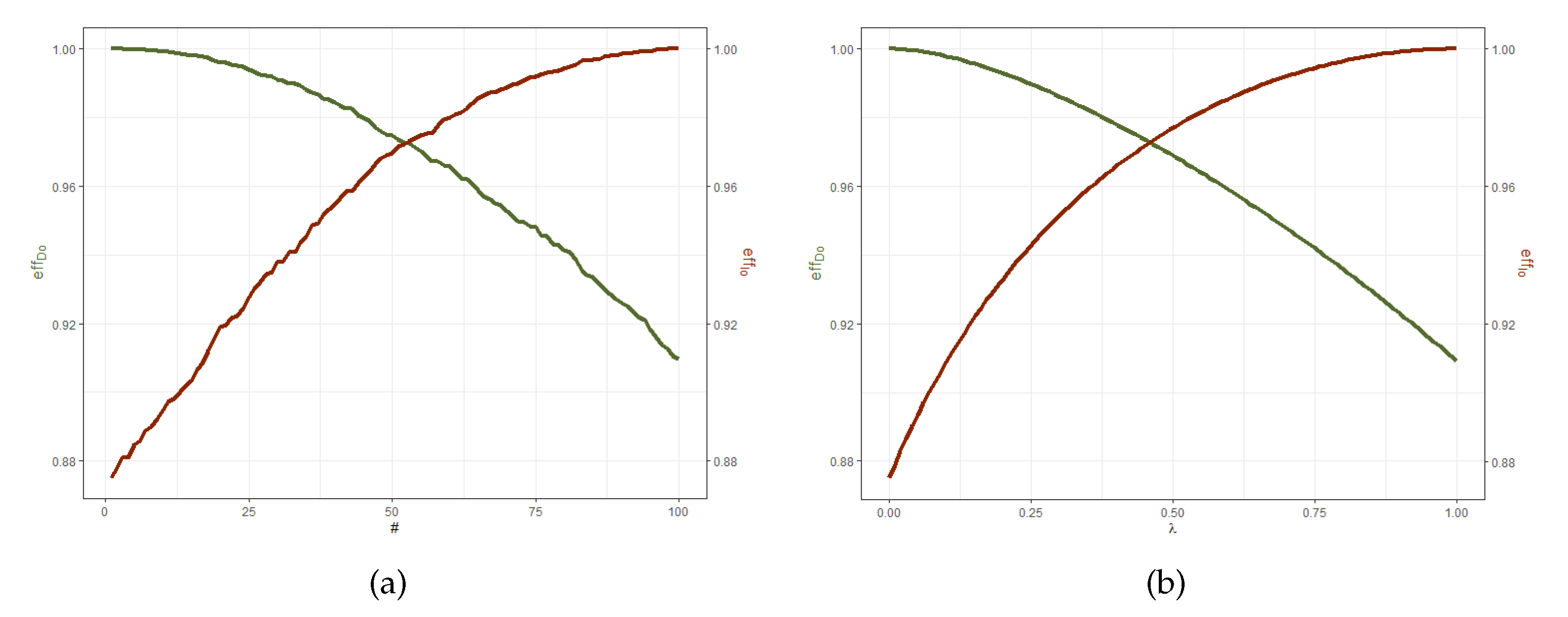
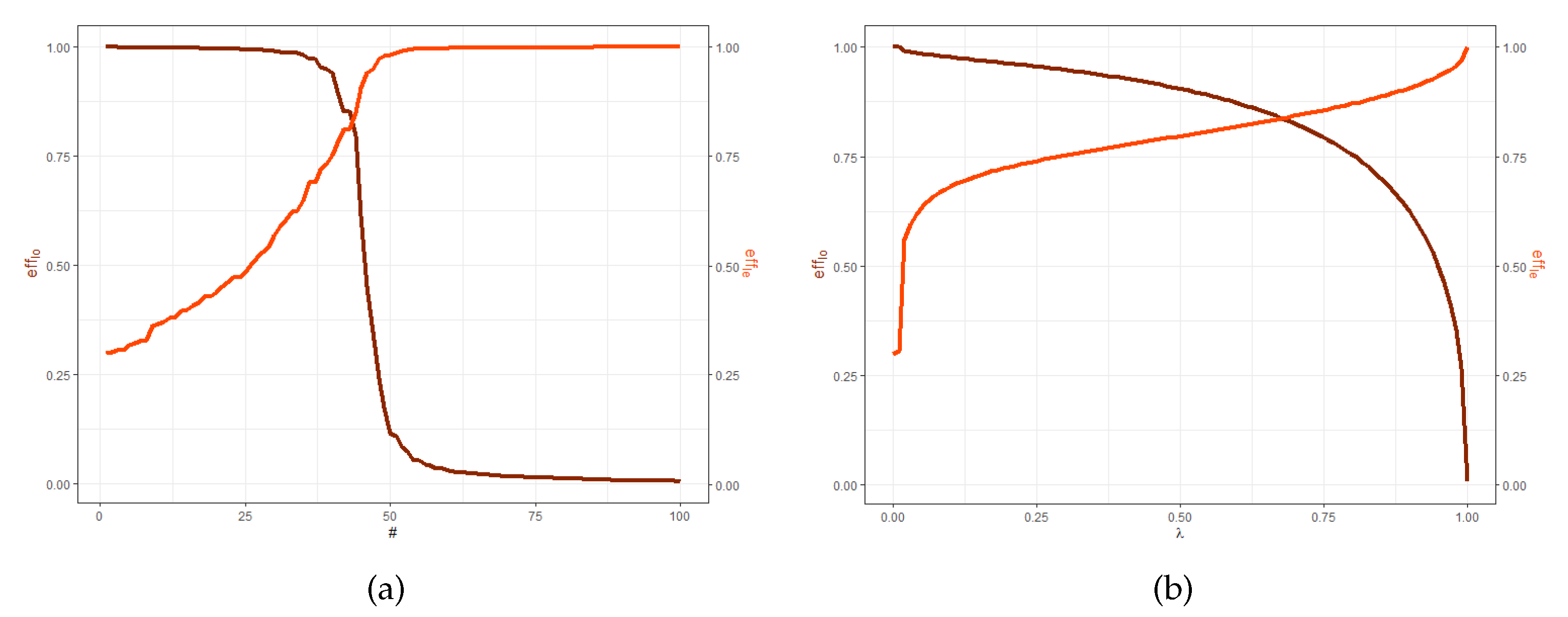
Having decided on an optimality criterion, the two designs can be compared via their efficiency. The efficiency for a criterion $\varphi$ is usually expressed with respect to the optimal design, ${\xi }_{\varphi }^{☆}$, and can be calculated from the following expression:

$${\mathrm{eff}}_{\varphi }\left(\xi \right)=\frac{\varphi \left[{\xi }_{\varphi }^{☆}\right]}{\varphi \left[\xi \right]},$$

(10)

with ${\xi }_{\varphi }^{☆}$ the $\varphi$-optimal design. Efficiency is usually expressed in terms of a percentage.

2.2. Dealing with Variance Structures and Optimisation Criteria

The dependence of the design on the model and the criterion is one of the main criticisms of the optimal experimental design theory [24]. This is clearly showcased in this application since just by changing the variance structure, without even changing the model, the performance of the designs for the alternative response has important losses in efficiency.

A suitable example is presented here in the cross efficiencies for the optimal designs for the Antoine Equation for water in the temperature range $\mathcal{X}={[1,100]}^{\circ }$C. Best guesses for the unknown parameters ${\theta }^0$ were obtained from [8], i.e., ${\theta }^{\left(0\right)}=(a,b,c)=(8.07131,1730.63,233.426)$. $D-$ and $I-$optimal designs for the homoscedastic, ${\xi }_{Do}^{☆}$ and ${\xi }_{Io}^{☆}$, and heteroscedastic, ${\xi }_{De}^{☆}$ and ${\xi }_{Ie}^{☆}$, models can be computed with the R package optedr [25].

Table 1. Cross efficiencies, in percentage, of the D- and I-optimal designs using ${\varphi }_I$ and ${\varphi }_D$ for the homoscedastic and heteroscedastic models.

	${\mathit{\xi }}_{\mathit{D}\mathit{o}}^{☆}$	${\mathit{\xi }}_{\mathit{I}\mathit{o}}^{☆}$			${\mathit{\xi }}_{\mathit{D}\mathit{e}}^{☆}$	${\mathit{\xi }}_{\mathit{I}\mathit{e}}^{☆}$
${\mathrm{eff}}_{Do}$	100	93.1		${\mathrm{eff}}_{De}$	100	58.7
${\mathrm{eff}}_{Io}$	89.7	100		${\mathrm{eff}}_{Ie}$	58.1	100

and

Table 2. Cross efficiencies, expressed as percentages of the optimal designs for the homoscedastic and heteroscedastic models when the true variance structure changes. The first table presents efficiencies for ${\varphi }_D$ while the second does for ${\varphi }_I$.

	${\mathit{\xi }}_{\mathit{D}\mathit{o}}^{☆}$	${\mathit{\xi }}_{\mathit{D}\mathit{e}}^{☆}$			${\mathit{\xi }}_{\mathit{I}\mathit{o}}^{☆}$	${\mathit{\xi }}_{\mathit{I}\mathit{e}}^{☆}$
${\mathrm{eff}}_{Do}$	100	25.5		${\mathrm{eff}}_{Io}$	100	0.7
${\mathrm{eff}}_{De}$	18.7	100		${\mathrm{eff}}_{Ie}$	29.7	100

show the cross efficiencies. For instance, in Table 1, the I-efficiency of the D-optimal design for the homoscedastic model, ${\xi }_{Do}^{☆}$, is $89.7\%$, to predict with minimal variance in the region ${[80-120]}^{\circ }\mathrm{C}$, considering $\mu \left(T\right)$ as a uniform distribution, ${\mathrm{eff}}_{Io}\left({\xi }_{Do}^{☆}\right)$. Similarly, in Table 2, the wrong assumption of the model from using the D-optimal design for the homoscedastic model, ${\xi }_{Do}^{☆}$ produces an efficiency of $18.7\%$ when the variance structure is heteroscedastic, ${\mathrm{eff}}_{De}\left({\xi }_{Do}^{☆}\right)$.

When D- and I-optimal designs are compared in the homoscedastic model, they have reasonably good efficiency for the other criterion; however, the efficiency loss in the heteroscedastic case is higher. Moreover, when the variance structure is wrong, the efficiency drops drastically, going as low as $0.7\%$. This highlights the need for careful consideration of the probability distribution of the response, as well as the need to look for compromise solutions between different models and/or criteria when the issue cannot be resolved.

3. Methods

The large efficiency losses—shown by the example of attempting to evaluate the efficiency of an optimal design for another criterion or to acknowledge possible errors in the response variance structure—motivate a combined or multiple compromise approach.

Two ideas have been considered in this study. First, when choosing the objective function $\varphi$, the best estimation of the model parameters ${\varphi }_D$ and the best possible prediction in a given region ${\varphi }_I$ produce different optimal designs, and a compromise solution for both criteria is desired. Second, as the variance structure of the response is an open question [10], the large differences between the efficiencies of optimal designs under one of the assumptions if the response variance structure is misguided makes the use of combined or multiple approaches to address this uncertainty interesting.

These situations, with a range of different interests, lead us to compare two different approaches. On the one hand is the traditional approach in OED, which is to configure a new criterion as a linear combination of two criteria producing a Compound Criterion [26], and on the other hand, obtaining optimal designs using a multi-objective approach in which the two criteria are evaluated simultaneously, looking for non-dominated solutions.

3.1. Compound Designs

There are two other approaches to combining different criteria, producing the design with consideration for a number of optimisation criteria. One can either combine two criteria, minimising the function value of one of them subject to a restriction of a minimum efficiency value for the second, or blend both criteria, considering a linear combination of their criteria functions (which is, in turn, also a criterion function). Cook and Wong [26] prove the equivalence of these two options, the constrained optimisation and the linear combination of several criteria.

If the experiment must comply with two different objectives given by two convex criteria functions, ${\varphi }_1$ and ${\varphi }_2$, representing main and secondary objectives, respectively, defined over all the possible designs for a given model, $\xi \in \mathrm{\Xi }$, we can combine the two criteria by selecting a criterion that minimises the value of the secondary criterion, constrained to a pre-established minimum efficiency for the first one:

$$min{\varphi }_2\left(\xi \right)\mathrm{subject}\mathrm{to}{\varphi }_1\left(\xi \right)\le c.$$

(11)

The restriction of one criterion to another is proved to be equivalent to considering a single compound criterion from the primary and secondary criteria, considering a criterion function based on a linear combination of the criterion functions ${\varphi }_1$ and ${\varphi }_2$,

$$\varphi (\xi \mid \lambda )=\lambda {\varphi }_1\left(\xi \right)+(1-\lambda ){\varphi }_2\left(\xi \right),$$

(12)

with $0\le \lambda \le 1$ a chosen constant Atkinson et al. [15]. The value of this constant, $\lambda$, represents the weight or relative importance assigned to each criterion. If $\lambda$ is close to one, the preference leans toward the criterion ${\varphi }_1$, while choosing a value close to zero shifts the efficiency towards the second criterion, ${\varphi }_2$.

3.2. Multi-Objective Approach

A multi-objective optimisation problem with q objectives can be defined as follows:

$$minimise\{f_1\left(\mathbf{x}\right),f_2\left(\mathbf{x}\right),\cdots ,f_q\left(\mathbf{x}\right)\}\mathrm{subject}\mathrm{to}\mathbf{x}\in X,$$

(13)

where $f_i,i=1,\cdots ,q$$(q\ge 2)$ are the possibly conflicting objective functions that must be minimised simultaneously, and X is the set of all feasible solutions. In our particular study, $q=2$, we consider two objective functions.

The dominance-based solution methods are very interesting ways of tackling multi-objective problems, OED-related or not. In particular, when two objective functions $f_1$ and $f_2$ are to be minimised, a solution S is Pareto dominated, or simply dominated by a solution $S^{\prime }$ (denoted by $S^{\prime }\prec S$), if and only if $f_1\left(S^{\prime }\right)\le f_1\left(S\right)$ and $f_2\left(S^{\prime }\right)<f_2\left(S\right)$, or $f_1\left(S^{\prime }\right)<f_1\left(S\right)$ and $f_2\left(S^{\prime }\right)\le f_2\left(S\right)$, i.e., $S^{\prime }$ is better in at least one objective function and is never worse in any objective function.

It usually happens that a unique solution cannot be optimal with respect to both objectives. In this study, we are looking for the set of all non-dominated solutions or Pareto optimal solutions. These solutions are not dominated by any solution $S^{\prime }\in X$, and so the improvement of one objective necessarily implies the worsening of the other objective. The Pareto front $P{S}^{*}$ is defined as the set of all objective function values corresponding to the solutions in the Pareto optimal set.

The advantage of algorithms that return a set of non-dominated solutions is the flexibility they allow in the choice of preferred solution and also the possibility to study how the different criterion functions grow and decay, which can lead to more informed choices.

In this paper, we will consider a hybrid multi-objective metaheuristic, which is detailed in the following Section.

4. Memetic Algorithms

Genetic algorithms (GAs) are among the many nature-inspired algorithms developed in recent decades. They were first presented by John Holland at the University of Michigan [27].

Metaheuristics, in general, were quickly adopted by the scientific community due to their ease of adaptation to a wide array of problems, as few to no assumptions about the objective function are needed. Due to a high success rate in finding optimal or good enough solutions to complex optimisation problems in engineering and computer science, their popularity has increased to the point of surpassing traditional optimisation methods [28].

A wide array of metaheuristics have been applied to solve optimal experimental design problems. Approaches as diverse as simulated annealing [29] or the imperialist competitive algorithm [30] have been used to find optimal designs. Several studies use the particle swarm optimisation metaheuristic originally proposed in [31], solving problems such as standardised maximin D-optimal designs [32] or minimax optimal designs [33]. Genetic algorithms have also been used quite extensively for a number of design issues, such as generating sequential space-filling designs [34], finding near-optimal Bayesian designs [35], constructing exact designs for mixture experiments [21], or calculating multi-objective optimal designs [36]. Some broader comparisons between different metaheuristics and deterministic algorithms have been explored in García-Ródenas et al. [37].

Although there is no guarantee that metaheuristic algorithms will arrive at the optimal solution, they have proven to be highly effective when applied to very different problems. However, a lack of a proven convergence to the optimal solution might be the reason why the use of metaheuristics lags behind in statistics compared to other sciences.

4.1. Single-Objective Memetic Algorithm

This paper introduces an evolutionary algorithm hybridised with a local search method in order to mimic “memetic evolution” [38]. This proposal combines several ideas from the literature, adapted to design a competitive algorithm for this particular problem.

Conventional GAs often produce moderate results, but meaningful improvements can be obtained through hybridisation with other methods. One such technique is local search, and in this case, the hybrid GA is usually called a memetic algorithm, as the biological evolution is changed by a cultural evolution where chromosomes might be modified before being included in subsequent generations. The hybridisation can be carried out by applying the local search algorithm to every chromosome immediately after it is generated instead of simply applying the decoding algorithm, as is the case for a plain genetic algorithm.

Algorithm 1 shows the structure of the memetic algorithm considered herein. In the first step, an initial population is randomly generated and improved with a local search (see Section 4.1.7). Then the algorithm iterates over a number of steps or generations until a stopping criterion is satisfied, which consists of a number of consecutive generations without improving the best solution found so far.

In each iteration, a new generation is built from the previous generation by applying the genetic operators of selection, crossover, and replacement. At the selection phase, all chromosomes are randomly grouped into pairs (and so every solution is a parent exactly once), and each of these pairs is mated to obtain two offspring. The mutation operator is then applied to these offspring with some probability, and finally, local search is used to improve them (see Section 4.1.7). Then, the replacement strategy is carried out to choose chromosomes for the next generation. Local search is again applied to the best solution in the population in order to further increase the intensification aspect of the algorithm. Additional details of the algorithm are given in the following subsections.

Algorithm 1 The memetic algorithm

Require: A scheduling problem instance P Ensure: A schedule H for instance P    Generate the initial population of size $popSize$;    Apply $LSiterations$ iterations of local search to every chromosome;    while No termination criterion is satisfied do       Group chromosomes randomly into pairs;       Apply the crossover operator to each pair with probability $crProb$;       Apply the mutation operator to each chromosome with probability $mutProb$;       Apply $LSiterations$ iterations of local search to every generated offspring;       Choose chromosomes for the next generation with the replacement strategy;       Apply $LSiterations$ iterations of local search to the best solution in the population;    end while    return The schedule from the best chromosome;

4.1.1. Solution Representation

We have decided to use variable-length chromosomes to codify a solution. In particular, each chromosome $Cx$ will be a number of points $C{x}_p$ with their respective weights $C{x}_w$. Evidently, the sum of all weights of the chromosome must be one.

Moreover, we always maintain the chromosome ordered from the lowest to the highest point. The advantages are twofold: regarding the implementation, operations on the chromosome have less complexity, and regarding the performance, the search space is reduced (note that if not ordered, the same design has as many as $n!$ different chromosomes, where n is the number of points of the design).

In a solution, the minimum number of points allowed ($minPoints$) is set by the number of parameters m (3 in our experiments), as it is not possible to estimate m parameters with fewer than m points, and in fact, this would result in a singular information matrix, which is not possible for the criteria considered. The maximum number of points allowed ($maxPoints$) is calculated by $m·(m+1)/2+1$ (see Section 2.1.1), which is 7 in our experiments.

We give two example chromosomes C1 and C2:

$C{1}_p$ = $12.41$	$31.17$	$44.40$	$78.81$	$100.00$
$C{1}_w$ = $0.08$	$0.18$	$0.40$	$0.23$	$0.11$
$C{2}_p$ = $32.17$	$41.24$	$74.20$	$96.35$
$C{2}_w$ = $0.53$	$0.05$	$0.20$	$0.22$

4.1.2. Generation of the Initial Population

We choose to initialise the population with random solutions. In particular, for each chromosome, a random number of points between $minPoints$ and $maxPoints$ is created. Each point is randomly chosen between ${\min }_{\mathcal{X}}$ and ${\max }_{\mathcal{X}}$ (i.e., the minimum and maximum of the design space $\mathcal{X}$) and its weight is also random between 0 and 1 (at the end the weights are divided so that the sum of all weights is one). Finally, we check whether the number of “different points” is higher than $minPoints$. If it is not, we discard this possible solution and repeat the process. Two points are considered to be not different if they are “very close,” and the threshold is set beforehand by a parameter, set at $1.0$ in our experiments.

4.1.3. Evaluation of a Chromosome

To evaluate a chromosome that represents a design, some checks are first performed. First, we eliminate all the points with “very low” weight (minimum weight is controlled by a parameter and is set to $0.001$ in these experiments). Second, if there are two points that are “very close,” we merge them in a single point halfway between both that has the sum of both weights (minimum admissible distance is controlled by a parameter and is set to $1.0$ in our experiments).

Now, after these adjustments, we check how many points the chromosome finally has. If the number is lower than $minPoints$, we assign the worst possible fitness to the solution. In practice, this eliminates it, preventing it from advancing to the next generation of the genetic algorithm.

In the other case, the design is finally evaluated, depending on the chosen optimisation criteria.

4.1.4. Crossover

The crossover operator is usually the most important operator of a genetic algorithm, as it should generate individuals that inherit good characteristics from their parents and hopefully create good solutions. For our problem, the idea is to swap some of the points in the crossover step and then give the mutation and local search the task of modifying the weights.

An example will clarify how the crossover works. Let the parents $C1$ and $C2$ be the example chromosomes given in Section 4.1.1. First, randomly decide the number of swaps between the chromosomes between 1 and the minimum number of points of both chromosomes minus 1, so between 1 and 3 in this example.

That number of random points is then swapped. In our example, suppose that two swaps are performed, the first swaps the second point of C1 with the third point of C2, and the second one swaps the first point of C1 with the second point of C2. In this case, the following two offspring solutions O1 and O2 are obtained:

$O{1}_p$ = $41.24$	$44.40$	$74.20$	$78.81$	$100.00$
$O{1}_w$ = $0.08$	$0.40$	$0.18$	$0.23$	$0.11$
$O{2}_p$ = $12.41$	$31.17$	$32.17$	$96.35$
$O{2}_w$ = $0.05$	$0.20$	$0.53$	$0.22$

4.1.5. Mutation

Mutation operators are used to preserve and improve the diversity of the population. This paper extends the BGA mutation operator [39], well-known for its good performance in real-coded genetic algorithms.

Applying the mutation to a chromosome, first, a random decision is taken as to whether to modify one random weight or one random point (0.5 probability each).

The BGA mutation operator works as follows: if $c_i\in [a_i,b_i]$ is a value to be mutated, the resulting value $c_i^{\prime }$ is,

$$c_i^{\prime }=c_i\pm ran{g}_i\times \sum _{k=0}^{15}{\alpha }_k{2}^{-k}.$$

(14)

where $ran{g}_i$ defines the mutation range and is set to $0.1\times (b_i-a_i)$. The + or – sign is chosen with a probability of 0.5, and ${\alpha }_i\in \{0,1\}$ is randomly generated with $p({\alpha }_i=1)=1/16$.

In case of a point mutation, clearly, the mutated point should not be lower than ${\min }_{\mathcal{X}}$ or higher than ${\max }_{\mathcal{X}}$. A similar check is carried out if a weight is mutated, and in this last case, another random weight must also be modified in the opposite direction so that the total sum of weights remains one.

4.1.6. Replacement Strategy

The replacement strategy is taken from [40]. It is based on preselection schemes, which are intended to improve diversity and prevent premature convergence. In particular, for each pair of parents and their two offspring, the best two chromosomes are selected for the next generation, such that they have a different value for the fitness function.

4.1.7. Local Search

Local search is a successful metaheuristic that is implemented by defining the neighbourhood of each point in the search space as the set of solutions reachable by a given transformation rule. It is useful in providing intensification in the search, which perfectly complements the diversification ensured by a genetic algorithm.

For this study, some classical local search could have been used, with provable convergence (albeit usually very slow) to the optimal solution, such as, for example, that proposed in [41]. However, in this case, the local search is embedded in the genetic algorithm. Hence it cannot be computationally expensive as it will be executed many times in each run.

For this reason, a simpler approach is proposed based on the BGA mutation operator previously described in Section 4.1.5. The idea is to perform a fixed number of iterations for each chromosome, each iteration consisting of the following steps:

• Apply the mutation operator to the chromosome.
• Check the fitness of the mutated solution.
• If the mutated solution is better, substitute the current chromosome for the mutated chromosome, and if not, keep the mutated chromosome.

The intensity of the local search can be controlled by modifying the parameter $LSiterations$, which sets the number of local search iterations per chromosome.

The intention is to apply this local search to every chromosome in the initial population and also to each offspring generated. It is also applied to the best chromosome in each generation. Note that, as this local search is stochastic and not deterministic, it can make sense to apply it several times to the same chromosome.

4.2. About Compound Criteria Optimisation

To perform a compound criteria optimisation, the only modification to be made to the described algorithm is the evaluation function. In particular, both objectives and a combination of both are calculated (depending on the value of the parameter $\lambda$). Therefore, the single-objective memetic algorithm is run as many times as desired with different values of the parameter, depending on the number of designs sought.

4.3. Multi-Objective Dominance-Based Memetic Algorithm

A dominance-based hybrid metaheuristic is proposed, combining a genetic algorithm based on the NSGA-II framework [42] with a multi-objective local search method. NSGA-II is a well-known method used to solve many real applications; see, for example, [43].

The main difference between an NSGA-II-based multi-objective genetic algorithm and a standard single-objective genetic algorithm is the replacement strategy. The strategy proposed in [42] is adopted, which consists of selecting solutions from lower non-domination levels and using the crowding distance to break ties when not all solutions from a given level can advance to the next generation. In order to see full details of the procedure, we refer the interested reader to [42].

In order to improve the diversity of the new population, we remove duplicated-fitness individuals from the pool of solutions before applying the replacement strategy. This procedure is used in several papers, for example, [44].

Besides the replacement step, the selection operator is also modified: instead of grouping the population in random pairs, a tournament selection is performed with size 2 (for selecting each parent, two chromosomes are taken at random from the population and the best-chosen for mating). It is empirically checked that, in the NSGA-II case, this selection operator performs better.

Multi-Objective Local Search

Designing multi-objective local searchers is difficult, as the dominance relation ≺ only defines a partial order, and so selecting the “best” neighbour is not trivial. This study takes the multi-objective hill-climbing local search method proposed in [44,45], which is fast and efficient and is specifically designed to be combined with a multi-objective genetic algorithm.

The selection of the best neighbour is based on the dominance relation, but it also considers the current set of non-dominated solutions of the population of the genetic algorithm. Hence, when choosing whether to keep the mutated solution $S^{\prime }$ or the original solution S (see Section 4.1.7), we choose to keep $S^{\prime }$ if it satisfies at least one of the following requirements:

• $S^{\prime }\prec S$.
• $\nexists S1\in P$ such that $S\prec S1$ and $\exists S2\in P$ such that $S^{\prime }\prec S2$, where P is the set of non-dominated solutions of the current population of the genetic algorithm.

The second requirement allows the local search to select a neighbour even if it does not strictly dominate the current solution. It allows the selection of neighbours able to improve the current set of non-dominated solutions of the genetic algorithm, should the current solution be unable to improve that set.

In a similar way to the single-objective case, a local search is applied to every initial solution and to each generated offspring. However, in the multi-objective case, an extra local search is not applied to the best solution of the population, as there is no single best solution, and applying it to every non-dominated solution would unacceptably increase the intensification aspect of the algorithm and the percentage of time devoted to local search.

4.4. Computational Complexity

As pointed out in [46], there are several reasons to conclude that it is difficult to measure the time complexity of multi-objective evolutionary algorithms; however it is important to examine it. According to [42], one generation of NSGA-II has complexity $O(M\times N^2)$, which is governed by the non-dominated sorting part of the algorithm. M is the number of objectives (2 in our particular problem), and N is the population size. On the other hand, one generation of the single-objective genetic algorithm is on the order of $O\left(N\right)$. Additionally, the computational complexity of the proposed hill climbing single-objective local search is $O(LSiterations\times N)$ for each generation of the memetic algorithm, where $LSiterations$ is the number of iterations of local search per chromosome, whereas the complexity of the proposed multi-objective local search is $O(LSiterations\times M\times N^2)$ for each generation. Notice that in this case, N is squared because when deciding to accept a neighbour, we may have to check, in the worst case, all the non-dominated solutions of the population of the genetic algorithm, which might be the entire population. With the above, we can conclude that the overall complexity of our multi-objective memetic algorithm is on the order of $O(n_{gen}\times LSiterations\times M\times N^2)$ where $n_{gen}$ is the total number of generations performed. On the other hand, the complexity of the compound designs is $O(n_{runs}\times n_{gen}\times LSiterations\times N)$, where $n_{runs}$ is the number of runs of the genetic algorithm (i.e., how many designs we want). If we take $n_{runs}=N$ in order to obtain a similar number of solutions as the multi-objective memetic algorithm, then we see that the complexities of both methods are on the same order.

5. Results

The memetic algorithm described in Section 4 is used to solve the problems described in the introduction of this paper: low efficiencies when considering two different optimality criteria or lack of certainty about variance structure. The latter case is of particular interest, as the efficiency loss is larger.

The algorithms are implemented in C++ using a single thread, and the experiments were carried out on an Intel Core i5-2450M CPU at 2.5 GHz with 4 GB of RAM (Santa Clara, CA, USA), running on Windows 10 Pro (Redmond, WA, USA). The source code of all implemented methods is openly available online, and further details can be found in Supplementary Materials so that the research community is able to reproduce the results.

5.1. Parameter Analysis of the Memetic Algorithm

In a preliminary parametric analysis, some values for the parameters of the evolutionary metaheuristic were tested in order to find a satisfactory configuration.

Table 3. Results of the parametric analysis for the evolutionary metaheuristic, showing the values tested and, in bold, the best configuration found.

Parameter	Values Tested
$popSize$	50, 100, 200
$LSiterations$	5, 10, 30
$crProb$	0.6, 0.8, 1.0
$mutProb$	0, 0.1, 0.2, 0.3

summarises the tested values, indicating in bold the configuration that achieved the best average results for the single-objective version of the algorithm.

A maximum of 100 consecutive generations without improving the best solution is taken as a stopping criterion. These values result in reasonable convergence patterns.

Moreover, with these parameters, the running time of the proposal is less than 1 s per run, and so, is quite reduced.

5.2. Performance of the Algorithm: Efficiencies

On the one hand, for each of the situations described in Table 1 and Table 2, the single-objective memetic algorithm was used to calculate 100 compound designs, taking values of $\lambda$ from 0 to 1 in uniform steps. On the other, a single run of the multi-objective memetic algorithm was performed with a population size of 100 solutions. In order for the comparison to be fair, the stopping criterion of the multi-objective algorithm is adjusted so that its running time is similar to that of the combined running time of the 100 runs of the single objective algorithm.

Figure 1 shows the results for D-optimality (in green) and I-optimality (in red) in the homoscedastic model. The left-hand figure shows the Pareto front provided by the multi-objective algorithm, sorted by efficiency, while the right shows the combined results of the compound criterion for the different $\lambda$.

Figure 2 shows the results of the algorithms for I-optimality when there is uncertainty about the variance structure, homoscedastic (in dark red) and heteroscedastic (in light red).

The compromise efficiencies for the results of all cases considered are shown in

Table 4. Efficiencies of the most balanced solutions of the multi-objective algorithm ${\xi }_M^{☆}$, and compound criterion ${\xi }_C^{☆}$, for D- and I-optimality criteria in each variance structure.

	${\mathit{\xi }}_{\mathit{M}}^{☆}$	${\mathit{\xi }}_{\mathit{C}}^{☆}$			${\mathit{\xi }}_{\mathit{M}}^{☆}$	${\mathit{\xi }}_{\mathit{C}}^{☆}$
${\mathrm{eff}}_{Do}$	97.24	97.33		${\mathrm{eff}}_{De}$	88.66	88.64
${\mathrm{eff}}_{Io}$	97.29	97.23		${\mathrm{eff}}_{Ie}$	88.16	88.56

and

Table 5. Efficiencies of the most balanced solutions of the multi-objective algorithm ${\xi }_M^{☆}$, and compound criterion ${\xi }_C^{☆}$, for each structure of variance, for each of D- and I-optimality.

	${\mathit{\xi }}_{\mathit{M}}^{☆}$	${\mathit{\xi }}_{\mathit{C}}^{☆}$			${\mathit{\xi }}_{\mathit{M}}^{☆}$	${\mathit{\xi }}_{\mathit{C}}^{☆}$
${\mathrm{eff}}_{Do}$	80.35	84.73		${\mathrm{eff}}_{Io}$	85.22	83.77
${\mathrm{eff}}_{De}$	87.22	84.92		${\mathrm{eff}}_{Ie}$	81.23	83.76

. These represent the solution of the multi-objective algorithm (first column) and that of the compound design (second column) that produce more balanced efficiencies, i.e., a smaller difference between them. In the multi-objective case, we choose the solution whose representation in Figure 1 and Figure 2 would appear to be closer to where the efficiencies cross. For the compound designs, the $\lambda$ that favours this choice has been chosen.

Table 4 (left) reports the efficiencies of compromise designs when the homoscedastic model is considered for the D- and I-optimality, whereas Table 4 (right) shows the analogous efficiencies for the heteroscedastic model. Table 5 (left) shows the D-efficiencies considering both the homoscedastic and heteroscedastic model, whereas Table 5 (right) reflects the results in terms of I-optimality.

Comparing multiobjective algorithms is not trivial, and in fact, there is a large number of papers about the best way to compare them. In this work, we can consider solutions as points in a 2-dimension space where we represent a different efficiency in each axis. We propose to use the hypervolume indicator [47] (to be maximised), which is the most used in the literature [48]. It can be defined as the area of the set of points relative to a reference point, which in this work, we take point (0,0) as it corresponds to the worst possible efficiencies.

Table 6. Hypervolumes of the Pareto fronts returned by the multi-objective algorithm ${\xi }_M^{☆}$, and compound criterion ${\xi }_C^{☆}$, for each of the four considered cases.

	${\mathit{\xi }}_{\mathit{M}}^{☆}$	${\mathit{\xi }}_{\mathit{C}}^{☆}$
$Do-De$	0.908411	0.926677
$Do-Io$	0.997920	0.997985
$De-Ie$	0.965272	0.966263
$Io-Ie$	0.889778	0.901478

shows the hypervolume values of the Pareto fronts of both algorithms in each of the four considered cases. The compound criterion achieves slightly better results in all cases, although in half of them, the difference is negligible.

6. Conclusions

It has been seen that both the compound criteria and the multi-objective approach produce an increase in efficiencies that solve the two mentioned issues. First, the choice of optimisation criteria allows precise estimation of the model parameters through the D-optimisation and an accurate prediction through the I-optimisation. Second, a design that obtains high efficiencies for both variance structures in the homoscedastic and in the heteroscedastic scenario.

This paper showcases the usefulness of metaheuristic algorithms for obtaining optimal designs in the traditional approach of optimal design of experiments, regardless of the selected criterion or the variance structure of the response.

Both approaches (compound designs and multi-objective algorithm) provide quite similar results in terms of design efficiencies for the considered criteria and variance structures. The advantage of the multi-objective approach is that a single execution of the algorithm provides a unified Pareto front that, although less smooth, would have better scalability in more complex cases, for example, if we increased the number of objectives to be combined.

We believe that the main reasons for the good performance of our algorithm are the proper balance of the diversification provided by the genetic algorithm and the intensification provided by the local search.

One possible avenue for future work is to improve the metaheuristic approach, for example, by devising a more advanced local search that takes into account the sensitivity function in order to better guide it to promising regions of the search space, even if its computational complexity would be much higher. It could also be interesting to design a decomposition-based multi-objective metaheuristic, for example, MOEA/D [49], which might be more appropriate for the problem at hand. Studying the use of metaheuristics to obtain minimax or maximin designs is also relevant.

References

1. Wisniak, J. Historical Development of the Vapor Pressure Equation from Dalton to Antoine. J. Phase Eq. 2001, 22, 622–630. [Google Scholar] [CrossRef]
2. Poling, B.E.; Prausnitz, J.M.; O’Connell, J.P. The Properties of Gases and Liquids; McGraw Hill Professional: New York, NY, USA, 2001. [Google Scholar]
3. Wood, D.A. Predicting saturated vapor pressure of LNG from density and temperature data with a view to improving tank pressure management. Petroleum 2020, 7, 91–101. [Google Scholar] [CrossRef]
4. Medeiros, H.A.D.; Chiavone-Filho, O.; Rios, R.B. Influence of estimated physical constants and vapor pressure for esters in the methanol/ethanol recovery column for biodiesel production. Fuel 2020, 276, 118040. [Google Scholar] [CrossRef]
5. Alam, M.S.; Nikolova, I.; Singh, A.; MacKenzie, A.R.; Harrison, R.M. Experimental vapour pressures of eight n-alkanes (C17, C18, C20, C22, C24, C26, C28 and C31) measured at ambient temperatures. Atmos. Environ. 2019, 213, 739–745. [Google Scholar] [CrossRef]
6. Gaspar, D.J.; Phillips, S.D.; Polikarpov, E.; Albrecht, K.; Jones, S.; George, A.; Landera, A.; Santosa, D.M.; Howe, D.T.; Baldwin, A.G.; et al. Measuring and predicting the vapor pressure of gasoline containing oxygenates. Fuel 2019, 243, 630–644. [Google Scholar] [CrossRef]
7. Wang, W.; Wang, G.; Chen, G.; Chen, S.; Huang, Z. The effect of sulfur vapor pressure on Cu2ZnSnS4 thin film growth for solar cells. Sol. Energy 2017, 148, 12–16. [Google Scholar] [CrossRef]
8. Dortmund Data Bank. 2022. Available online: http://www.ddbst.com. (accessed on 1 December 2022).
9. Ford, I.; Tittterington, D.M.; Kitsos, C.P. Recent Advances in nonlinear experimental design. Technometrics 1989, 31, 49–60. [Google Scholar] [CrossRef]
10. Brozena, A.; Davidson, C.E.; Schlindler, B.; Tevault, D.E. Vapor Pressure Data Analysis and Statistics; Technical Report ECBC-TR-1422; Edgewood Chemical Biological Center, U.S. Army RDECOM: Aberdeen Proving Ground, MD, USA, 2016. [Google Scholar]
11. de la Calle-Arroyo, C.; López-Fidalgo, J.; Rodríguez-Aragón, L.J. Optimal Designs for Antoine Equation. Chemom. Intell. Lab. Syst. 2021, 214, 104334. [Google Scholar] [CrossRef]
12. Fedorov, V.V.; Hackl, P. Model-Oriented Design of Experiments; Lecture Notes in Statistics; Spinger: New York, NY, USA, 1997. [Google Scholar]
13. Kiefer, J. Optimum experimental designs. J. R. Stat. Soc. Ser. B 1959, 21, 272–319. [Google Scholar] [CrossRef]
14. Silvey, S.D. Optimal Design; Chapman & Hall: London, UK, 1980. [Google Scholar]
15. Atkinson, A.; Donev, A.; Tobias, R. Optimum Experimental Designs, with SAS; Oxford Statistical Science Series; OUP: Oxford, UK, 2007. [Google Scholar]
16. Fedorov, V.; Leonov, S. Optimal Design for Nonlinear Response Models; Chapman & Hall/CRC Biostatistics Series; Taylor & Francis: Boca Raton, FL, USA, 2014. [Google Scholar]
17. Wald, A. On the efficient design of statistical investigations. Ann. Math. Stat. 1943, 14, 134–140. [Google Scholar] [CrossRef]
18. Coetzer, R.; Haines, L.M. The construction of D- and I-optimal designs for mixture experiments with linear constraints on the components. J. Comput. Appl. Math. 2017, 171, 112–124. [Google Scholar] [CrossRef]
19. Harman, R.; Filová, L.; Richtárik, P. A Randomized Exchange Algorithm for Computing Optimal Approximate Designs of Experiments. J. Comput. Appl. Math. 2019, 115, 348–361. [Google Scholar] [CrossRef] [Green Version]
20. Goos, P.; Jones, B.; Syafitri, U. I-Optimal design of mixture experiments. J. Am. Stat. Assoc. 2016, 111, 899–911. [Google Scholar] [CrossRef]
21. Martín-Martín, R.; García Camacha, I. Efficient algorithms for constructing D- and I-optimal exact designs for linear and non-linear models in mixture experiments. Statist. Op Res. Trans. 2019, 43, 163–190. [Google Scholar] [CrossRef]
22. Kiefer, J. General Equivalence Theory for Optimum Designs (Approximate Theory). Ann. Stat. 1974, 2, 849–879. [Google Scholar] [CrossRef]
23. Kiefer, J.; Wolfowitz, J. The equivalence of two extremum problems. Can. J. Math. 1960, 12, 363–366. [Google Scholar] [CrossRef]
24. Pozuelo-Campos, S.; Casero-Alonso, V.; Amo-Salas, M. Strategies for robust designs in toxicological tests. Chemom. Intell. Lab. Syst. 2022, 225, 104560. [Google Scholar] [CrossRef]
25. de la Calle-Arroyo, C.; López-Fidalgo, J.; Rodríguez-Aragón, L.J. Optedr: Calculating Optimal and D-Augmented Designs, R package version 2.0.0. CRAN; R Foundation for Statistical Computing: Vienna, Austria, 2022; Available online: https://cran.r-project.org/package=optedr (accessed on 20 January 2023).
26. Cook, R.D.; Wong, W.K. On the equivalence of constrained and compound optimal designs. J. Am. Stat. Assoc. 1994, 89, 687–692. [Google Scholar] [CrossRef]
27. Holland, J.H. Adaptation in Natural and Artificial Systems: An Introductory Analysis with Applications to Biology, Control and Artificial Intelligence; The University of Michigan Press: Cambridge, MA, USA, 1975. [Google Scholar]
28. Whitacre, J. Survival of the flexible: Explaining the recent popularity of nature-inspired optimization within a rapidly evolving world. Computing 2011, 93, 135–146. [Google Scholar] [CrossRef]
29. Woods, D.C. Robust designs for binary data: Applications of simulated annealing. J. Stat. Comput. Simul. 2010, 80, 29–41. [Google Scholar] [CrossRef]
30. Masoudi, E.; Holling, H.; Wong, W.K. Application of imperialist competitive algorithm to find minimax and standardized maximin optimal designs. Comput. Stat. Data Anal. 2017, 113, 330–345. [Google Scholar] [CrossRef]
31. Kennedy, J.; Eberhart, R. Particle Swarm Optimization. In Proceedings of the IEEE International Conference on Neural Networks, Perth, WA, Australia, 27 November–1 December 1995; pp. 1942–1948. [Google Scholar]
32. Chen, P.Y.; Chen, R.B.; Tung, H.C.; Wong, W.K. Standardized maximim D-optimal designs for enzyme kinetic inhibition models. Chemom. Intell. Lab. Syst. 2017, 169, 79–86. [Google Scholar] [CrossRef] [Green Version]
33. Chen, R.B.; Chang, S.P.; Wang, W. Minimax optimal designs via particle swarm optimization methods. Stat. Comput. 2015, 25, 975–988. [Google Scholar] [CrossRef]
34. Crombecq, K.; Dhaene, T. Generating sequential space-filling designs using genetic algorithms and Monte Carlo methods. In Proceedings of the Lecture Notes in Computer Science; Deb, K., Bhattacharya, A., Chakraborti, N., Chakroborty, P., Das, S., Dutta, J., Gupta, S., Jain, A., Aggarwal, V., Branke, J., et al., Eds.; Springer: Berlin/Heidelberg, Germany, 2010; Volume 6457, pp. 80–84. [Google Scholar]
35. Hamada, M.; Martz, H.F.; Reese, C.S.; Wilson, A.G. Finding Near-Optimal Bayesian Experimental Designs via Genetic Algorithms. J. Am. Stat. Assoc. 2001, 55, 175–181. [Google Scholar] [CrossRef]
36. Kao, M.H.; Mandal, A.; Lazar, N.; Stufken, J. Multi-objective optimal experimental designs for event-related fMRI studies. NeuroImage 2009, 44, 849–856. [Google Scholar] [CrossRef] [PubMed]
37. García-Ródenas, R.; García-García, J.C.; López-Fidalgo, J.; Martin-Baos, J.A.; Wong, W.K. A comparison of general-purpose optimization algorithms for finding optimal approximate experimental designs. Comput. Stat. Data Anal. 2020, 144, 106844. [Google Scholar] [CrossRef]
38. Tavakkoli-Moghaddam, R.; Javadi, B.; Jolai, F.; Ghodratnama, A. A memetic algorithm for the flexible flow line scheduling problem with processor blocking. Comput. Oper. Res. 2011, 36, 402–414. [Google Scholar] [CrossRef]
39. Mühlenbein, H.; Schlierkamp-Voosen, D. Predictive models for the breeder genetic algorithm in continuous parameter optimization. Evol. Comput. 1993, 1, 25–49. [Google Scholar] [CrossRef]
40. González, M.A.; Vela, C.R. An efficient memetic algorithm for total weighted tardiness minimization in a single machine with setups. Appl. Soft Comput. 2015, 37, 506–518. [Google Scholar] [CrossRef]
41. Solis, F.J.; Wets, R.J.B. Minimization by random search techniques. Math. Oper. Res. 1981, 6, 19–30. [Google Scholar] [CrossRef]
42. Deb, K.; Pratap, A.; Agarwal, S.; Meyarivan, T. A Fast and Elitist Multiobjective Genetic Algorithm: NSGA-II. IEEE Trans. Evol. Comput. 2002, 6, 182–197. [Google Scholar] [CrossRef] [Green Version]
43. Cao, Y.; Dhahad, H.A.; Togun, H.; Hussen, H.M.; Rashid, T.A.; Anqi, A.E.; Farouk, N.; Issakhov, A. Exergetic and financial parametric analyses and multi-objective optimization of a novel geothermal-driven cogeneration plant; adopting a modified dual binary technique. Sustain. Energy Technol. Assess. 2021, 48, 101442. [Google Scholar] [CrossRef]
44. González, M.A.; Oddi, A.; Rasconi, R. Efficient Approaches for Solving a Multiobjective Energy-aware Job Shop Scheduling Problem. Fundam. Inform. 2019, 167, 93–132. [Google Scholar] [CrossRef]
45. González, M.A.; Oddi, A.; Rasconi, R. Multi-Objective Optimization in a Job Shop with Energy Costs through Hybrid Evolutionary Techniques. In Proceedings of the Twenty-Seventh International Conference on Automated Planning and Scheduling (ICAPS-2017), Pittsburgh, PA, USA, 18–23 June 2017; AAAI Press: Washington, DC, USA, 2017; pp. 140–148. [Google Scholar]
46. Rahman, C.M.; Rashid, T.A.; Ahmed, A.M.; Mirjalili, S. Multi-objective learner performance-based behavior algorithm with five multi-objective real-world engineering problems. Neural Comput. Appl. 2022, 34, 6307–6329. [Google Scholar] [CrossRef]
47. Zitzler, E.; Thiele, L. Multiobjective optimization using evolutionary algorithms—A comparative case study. In Parallel Problem Solving from Nature—PPSN V Proceedings; Springer: Berlin/Heidelberg, Germany, 1998; pp. 292–301. [Google Scholar]
48. Riquelme, N.; Von Lücken, C.; Baran, B. Performance metrics in multi-objective optimization. In Proceedings of the 2015 Latin American Computing Conference (CLEI), Arequipa, Peru, 19–23 October 2015; pp. 1–11. [Google Scholar]
49. Zhang, Q.; Li, H. MOEA/D: A Multiobjective Evolutionary Algorithm Based on Decomposition. Evol. Comput. IEEE Trans. 2007, 11, 712–731. [Google Scholar] [CrossRef]
Figure 1. Efficiencies for D-optimality (in green) and I-optimality (in red) in the homoscedastic model. (a) Multi-objective algorithm. (b) Compound criterion.
Mathematics 11 00693 g001
Figure 2. I-efficiencies for the homoscedastic model (in dark red) and heteroscedastic model (in light red). (a) Multi-objective algorithm. (b) Compound criterion.
Mathematics 11 00693 g002