New Results on Finite-Time Synchronization Control of Chaotic Memristor-Based Inertial Neural Networks with Time-Varying Delays

Abstract

In this work, we are concerned with the finite-time synchronization (FTS) control issue of the drive and response delayed memristor-based inertial neural networks (MINNs). Firstly, a novel finite-time stability lemma is developed, which is different from the existing finite-time stability criteria and extends the previous results. Secondly, by constructing an appropriate Lyapunov function, designing effective delay-dependent feedback controllers and combining the finite-time control theory with a new non-reduced order method (NROD), several novel theoretical criteria to ensure the FTS for the studied MINNs are provided. In addition, the obtained theoretical results are established in a more general framework than the previous works and widen the application scope. Lastly, we illustrate the practicality and validity of the theoretical results via some numerical examples.

1. Introduction

Neural networks (NNs) have garnered considerable attention from researchers, due to being widely applied in numerous different fields, such as cryptography, model identification, and signal processing [1,2,3,4,5,6,7]. The essential issues of these applications are to research the dynamical behaviors of NNs. As a significant dynamical property, synchronization has attracted wide-scale attention in recent years [8,9,10,11,12]. However, in the existing papers, most of these published works are connected with infinite-time synchronization, such as exponential synchronization and asymptotical synchronization [13,14,15]. Considering that the lifespan of biologies and apparatus is limited, we always desire to obtain faster or even finite-time convergent speed in practice. Hence, the investigation of FTS is more meaningful [16,17,18,19]. In the meantime, compared with the infinite-time synchronization of NNs, FTS has a better convergence rate and exhibits several other desirable features.

It is well known that conventional NNs are usually presented by first-order differential equations. In 1986, Westervelt and Babcock established the NNs with an inertial item by adding the inductors into the NNs’ model, which could be described by a second-order form [20]. Inertial neural networks (INNs) have evident engineering and biological backgrounds, and the dynamical properties of INNs are more complicated than conventional NNs [21,22,23,24]. Recently, some results on the dynamical behaviors of INNs, which include periodicity, stability, dissipativity and so on, have been presented [25,26,27,28,29]. With the application of INNs to various fields such as secure communication, signal processing and image encryption [30,31,32], some further studies of the INNs are essential and significant. Meanwhile, due to the inherent communication times between the neurons and the limited switching speed of amplifiers, the time delays unavoidably exist in the process of the implementation of INNs (see Figure 1a). However, it has been proved in many previous works that the existence of time delays may cause divergence, oscillation, and even instability of the system [33,34,35]. Hence, the dynamic analysis of INNs with mixed time-varying delays (MTVDs) is necessary for their successful applications.

On the other hand, a memristor device, which is the fourth basic circuit element (see Figure 1b) successfully manufactured by HP Laboratory [36], is a perfect element to simulate the function of the neural synapse [37,38]. Adopting memristors as the synapses connection weights in the circuit of NNs has a lot of merits, including simple structure, nano-dimension, ease of integration and low power consumption [39,40]. Considering the advantages of memristors, memristor-based INNs have become a hot topic [41,42,43,44]. In [45], by using a hybrid feedback controller, novel results were acquired to insure the FTS of drive and response MINNs, and the authors deeply discuss the relationship between the estimated value of settling time and the parameter ${\xi }_i$ in variable substitution. In [46], the authors investigated the FTS and fixed time synchronization of MINNs by using the Lyapunov stability theory and Filippov discontinuous theory. However, so far, all authors have studied the FTS of MINN by utilizing a variable substitution method to transform MINNs’ system into a first-order form. There are hardly any articles studying the dynamical properties of MINNs by using NROD, and the existing results are just focused on infinite-time synchronization or stability. As mentioned in the papers [28,41], the variable transformation method for the discontinuous MINNs’ system may be short of rigor in practice. Hence, researching MINNs themselves directly is a better method, instead of utilizing the reduced-order method.

Motivated by the aforementioned discussions, in this work, we will investigate the MINNs with MTVDs by using a new study method and acquire several new sufficient conditions to insure the FTS for such considered systems. The main contributions are highlighted below:

• A novel finite-time stability criterion is derived (see Lemma 2), which is different from the existing finite-time stability criteria and extends the previous results.
• By combining finite-time control theory with a new NROD, which can study MINNs themselves directly instead of using the variable substitution method, some new theoretical criteria to ensure the FTS for the studied MINNs are developed.
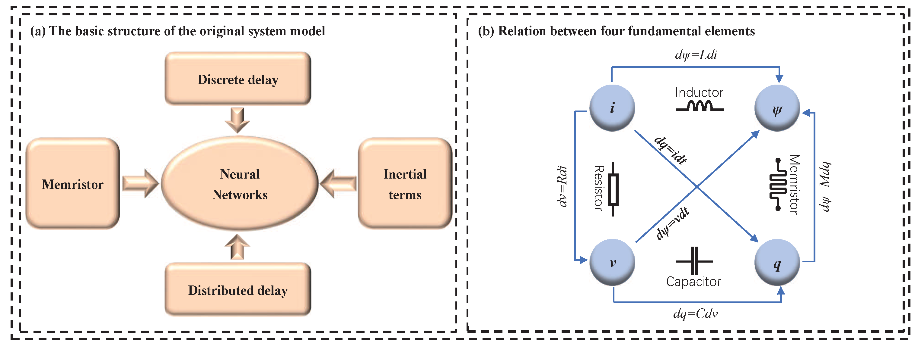
• Taking the memristors, inertial items, and MTVDs into account, the acquired theoretical results are established in a more general framework than the previous results and widens the application scope.

The remainder of this paper is organized as follows. In Section 2, the INNs model, some useful definition, and lemmas are introduced. In Section 3, new criteria for IMNNs with MTVDs derived are given. In Section 4, illustrative examples are presented to validate the effectiveness of the theoretical results. Finally, Section 5 shows the conclusions.

Notations: Let $\mathbb{R}$ denote the space of real numbers. $C([t_0-\tau ,t_0],\mathbb{R})$ denotes the set of all continuous functions from $[t_0-\tau ,t_0]$ to $\mathbb{R}.$ $x^T$ denotes the transpose of a vector (or a matrix) $x.$ $diag\{\dots \}$ denotes a diagonal matrix. ${(·)}_{n\times n}$ denotes a $n\times n$ matrix. $\left|\right|·{\left|\right|}_1$ are the 1-norm of a vector (or a matrix).

2. Preliminaries

In this work, we consider the MINNs with MTVDs as follows:

$$\begin{array}{cc}\hfill \frac{d^2{x}_i\left(t\right)}{d{t}^2}=& -a_i\frac{d{x}_i\left(t\right)}{dt}-b_i{x}_i\left(t\right)+\sum _{j=1}^n{c}_{ij}\left(x_i\left(t\right)\right)f_j\left(x_j\left(t\right)\right)+\sum _{j=1}^n{d}_{ij}\left(x_i\left(t\right)\right)\hfill \\ \hfill & \times f_j\left(x_j(t-\tau \left(t\right))\right)+\sum _{j=1}^n{e}_{ij}\left(x_i\left(t\right)\right){\int }_{t-\ell \left(t\right)}^t{f}_j\left(x_j\left(s\right)\right)ds+I_i\left(t\right)\hfill \end{array}$$

(1)

$i\in \{1,2,\dots ,n\},$ where $x_i\left(t\right)$ represents the state of the ith neuron, and the second derivative of $x_i\left(t\right)$ is called an inertial term of the system (1). $a_i>0$ and $b_i>0$ are constants. The function $f_j(·)$ represents the nonlinear activation function. $I_i\left(t\right)$ is the external input on the ith neuron. $\tau \left(t\right)$ and $\ell \left(t\right)$ are the discrete and distributed delay, respectively, and there exist constants $\tau$ and ℓ such that $0\le \tau \left(t\right)\le \tau ,$ $0\le \ell \left(t\right)\le \ell$. $c_{ij}\left(x_i\left(t\right)\right),$ $d_{ij}\left(x_i\left(t\right)\right)$ and $e_{ij}\left(x_i\left(t\right)\right)$ are memristor-based connection weights, which are given by

$$\begin{array}{cc}\hfill & c_{ij}\left(x_i\left(t\right)\right)=\left\{\begin{array}{c}{c}_{ij}^{\prime },\left|x_i\left(t\right)\right|\le T_i,\hfill \\ c_{ij}^{″},\left|x_i\left(t\right)\right|>T_i,\hfill \end{array}\right.d_{ij}\left(x_i\left(t\right)\right)=\left\{\begin{array}{c}{d}_{ij}^{\prime },\left|x_i\left(t\right)\right|\le T_i,\hfill \\ d_{ij}^{″},\left|x_i\left(t\right)\right|>T_i,\hfill \end{array}\right.e_{ij}\left(x_i\left(t\right)\right)=\left\{\begin{array}{c}{e}_{ij}^{\prime },\left|x_i\left(t\right)\right|\le T_i\hfill \\ e_{ij}^{″},\left|x_i\left(t\right)\right|>T_i\hfill \end{array}\right.\hfill \end{array}$$

for $i,j=1,2,\dots ,n,$ where $T_i>0$ represents the switching jumps, and $c_{ij}^{\prime },c_{ij}^{″},d_{ij}^{\prime },d_{ij}^{″},e_{ij}^{\prime },e_{ij}^{″},$ are known constants. Denote

$$\begin{array}{cc}\hfill & {\overline{c}}_{ij}=max\left\{\right|c_{ij}^{\prime }|,|c_{ij}^{″}\left|\right\},{\overline{d}}_{ij}=max\left\{\right|d_{ij}^{\prime }|,|d_{ij}^{″}\left|\right\},{\overline{e}}_{ij}=max\left\{\right|e_{ij}^{\prime }|,|e_{ij}^{″}\left|\right\},{\widehat{c}}_{ij}=max\{c_{ij}^{\prime },c_{ij}^{″}\},\hfill \\ & {\check{c}}_{ij}=min\{c_{ij}^{\prime },c_{ij}^{″}\},{\widehat{d}}_{ij}=max\{d_{ij}^{\prime },d_{ij}^{″}\},{\check{d}}_{ij}=min\{d_{ij}^{\prime },d_{ij}^{″}\},{\widehat{e}}_{ij}=max\{e_{ij}^{\prime },e_{ij}^{″}\},{\check{e}}_{ij}=min\{e_{ij}^{\prime },e_{ij}^{″}\}\hfill \end{array}$$

and

$$\begin{array}{cc}\hfill & \overline{C}={\left({\overline{c}}_{ij}\right)}_{n\times n},\overline{D}={\left({\overline{d}}_{ij}\right)}_{n\times n},\overline{E}={\left({\overline{e}}_{ij}\right)}_{n\times n},\widehat{C}={\left({\widehat{c}}_{ij}\right)}_{n\times n},\check{C}={\left({\check{c}}_{ij}\right)}_{n\times n},\hfill \\ \hfill & \widehat{D}={\left({\widehat{d}}_{ij}\right)}_{n\times n},\check{D}={\left({\check{d}}_{ij}\right)}_{n\times n},\widehat{E}={\left({\widehat{e}}_{ij}\right)}_{n\times n},\check{E}={\left({\check{e}}_{ij}\right)}_{n\times n}.\hfill \end{array}$$

The initial value of system (1) is given by

$$\begin{array}{c}\hfill x_i\left(s\right)={\varphi }_i\left(s\right),\frac{d{x}_i\left(s\right)}{ds}={\varphi }_i^{\prime }\left(s\right),t_0\ge 0,s\in [t_0-\tau ,t_0]\end{array}$$

where ${\varphi }_i\left(s\right),{\varphi }_i^{\prime }\left(s\right)\in C([t_0-\tau ,t_0],\mathbb{R}),$ $i=1,2,\dots ,n.$

For the activation functions $f_j(·),$ we conduct the following assumptions.

Assumption 1.

For $\forall x,y\in \mathbb{R},$ $x\ne y$, there exist constants $l_j>0$ such that the activation function $f_j:\mathbb{R}\to \mathbb{R}$ satisfies $|f_j\left(x\right)-f_j\left(y\right)|\le l_j|x-y|,i=1,2,\dots ,n,$ i.e., the function $f_j$ satisfies the Lipschitz condition,

Assumption 2.

For $\forall x\in \mathbb{R},$ there exist constants $M_j>0$ such that the activation function $f_j:\mathbb{R}\to \mathbb{R}$ satisfies $|f_j\left(x\right)|\le M_j,i=1,2,\dots ,n,$ i.e., the function $f_j$ is bounded.

Then, the response MINNs is given as follows:

$$\begin{array}{cc}\hfill \frac{d^2{y}_i\left(t\right)}{d{t}^2}=& -a_i\frac{d{y}_i\left(t\right)}{dt}-b_i{y}_i\left(t\right)+\sum _{j=1}^n{c}_{ij}\left(y_i\left(t\right)\right)f_j\left(y_j\left(t\right)\right)+\sum _{j=1}^n{d}_{ij}\left(y_i\left(t\right)\right)\hfill \\ \hfill & \times f_j\left(y_j(t-\tau \left(t\right))\right)+\sum _{j=1}^n{e}_{ij}\left(y_i\left(t\right)\right){\int }_{t-\ell \left(t\right)}^t{f}_j\left(y_j\left(s\right)\right)ds+I_i\left(t\right)+U_i\left(t\right)\hfill \end{array}$$

(2)

in which $y_i\left(t\right)$ is the state of the response MINNs and $U_i\left(t\right)$ is the properly designed controller; the memristor-based connection weights $c_{ij}\left(y_i\left(t\right)\right),$ $d_{ij}\left(y_i\left(t\right)\right),$ $e_{ij}\left(y_i\left(t\right)\right)$ are defined as in (1). The initial value of system (2) is as follows:

$$\begin{array}{c}\hfill y_i\left(s\right)={\psi }_i\left(s\right),\frac{d{y}_i\left(s\right)}{ds}={\psi }_i^{\prime }\left(s\right),t_0\ge 0,s\in [t_0-\tau ,t_0]\end{array}$$

where ${\psi }_i\left(s\right),{\psi }_i^{\prime }\left(s\right)\in C([t_0-\tau ,t_0],\mathbb{R}),$ $i=1,2,\dots ,n$.

Denote synchronization error $r_i\left(t\right)=y_i\left(t\right)-x_i\left(t\right).$ From (1) and (2), we obtain the error systems as follows:

$$\begin{array}{cc}\hfill \frac{d^2{r}_i\left(t\right)}{d{t}^2}=& -a_i\frac{d{r}_i\left(t\right)}{dt}-b_i{r}_i\left(t\right)+\sum _{j=1}^n{c}_{ij}\left(y_i\left(t\right)\right)g_j\left(r_j\left(t\right)\right)+\sum _{j=1}^n{d}_{ij}\left(y_i\left(t\right)\right)g_j\left(r_j(t-\tau \left(t\right))\right)\hfill \\ \hfill & +\sum _{j=1}^n{e}_{ij}\left(y_i\left(t\right)\right){\int }_{t-\ell \left(t\right)}^t{g}_j\left(r_j\left(s\right)\right)ds+\sum _{j=1}^n[c_{ij}\left(y_i\left(t\right)\right)-c_{ij}\left(x_i\left(t\right)\right)]f_j\left(x_j\left(t\right)\right)\hfill \\ \hfill & +\sum _{j=1}^n[d_{ij}\left(y_i\left(t\right)\right)-d_{ij}\left(x_i\left(t\right)\right)]f_j\left(x_j(t-\tau \left(t\right))\right)\hfill \\ \hfill & +\sum _{j=1}^n[e_{ij}\left(y_i\left(t\right)\right)-e_{ij}\left(x_i\left(t\right)\right)]{\int }_{t-\ell \left(t\right)}^t{f}_j\left(x_j\left(s\right)\right)ds+U_i\left(t\right)\hfill \end{array}$$

(3)

for $i=1,2,\dots ,n,$ where $g_j\left(r_j(·)\right)=f_j\left(y_j(·)\right)-f_j\left(x_j(·)\right)$.

The synchronization error system (3) can be transformed into the vector form as

$$\begin{array}{cc}\hfill r^{″}\left(t\right)=& -A{r}^{\prime }\left(t\right)-Br\left(t\right)+C_{y}g\left(r\left(t\right)\right)+D_{y}g\left(r(t-\tau \left(t\right))\right)+E_y{\int }_{t-\ell \left(t\right)}^{t}g\left(r\left(s\right)\right)ds\hfill \\ \hfill & +(C_y-C_x)f\left(x\left(t\right)\right)+(D_y-D_x)f\left(x(t-\tau \left(t\right))\right)\hfill \\ \hfill & +(E_y-E_x){\int }_{t-\ell \left(t\right)}^{t}f\left(x\left(s\right)\right)ds+U\left(t\right)\hfill \end{array}$$

(4)

where

$$\begin{array}{cc}\hfill & r\left(t\right)={\left(r_1\left(t\right),r_2\left(t\right),\dots ,r_n\left(t\right)\right)}^T,g\left(r(·)\right)={\left(g_1\left(r_1(·)\right),g_2\left(r_2(·)\right),\dots ,g_n\left(r_n(·)\right)\right)}^T,\hfill \\ \hfill & f\left(x(·)\right)={\left(f_1\left(x_1(·)\right),f_2\left(x_2(·)\right),\dots ,f_n\left(x_n(·)\right)\right)}^T,U\left(t\right)={\left(U_1\left(t\right),U_2\left(t\right),\dots ,U_n\left(t\right)\right)}^T.\hfill \end{array}$$

and

$$\begin{array}{cc}\hfill & A=\mathrm{diag}\{a_1,a_2,\dots ,a_n\},B=\mathrm{diag}\{b_1,b_2,\dots ,b_n\},C_y={\left(c_{ij}\left(y_i\left(t\right)\right)\right)}_{n\times n},C_x={\left(c_{ij}\left(x_i\left(t\right)\right)\right)}_{n\times n},\hfill \\ \hfill & D_y={\left(d_{ij}\left(y_i\left(t\right)\right)\right)}_{n\times n},D_x={\left(d_{ij}\left(x_i\left(t\right)\right)\right)}_{n\times n},E_y={\left(e_{ij}\left(y_i\left(t\right)\right)\right)}_{n\times n},E_x={\left(e_{ij}\left(x_i\left(t\right)\right)\right)}_{n\times n},\hfill \end{array}$$

The following definition and lemmas are given, which are helpful in proving the main results.

Definition 1.

[46] Drive and response MINNs (1) and (2) are said to be FTS, if for appropriate designed controller $U_i\left(t\right)$, there exists a constant $0<T<+\infty$, such that ${\displaystyle \underset{t\to t_0+T}{lim}r\left(t\right)=0,}$ and $r\left(t\right)\equiv 0$ for $\forall t\ge t_0+T,$ and T is called the settling time.

Since FTS requires that the system trajectories converge to a Lyapunov equilibrium state in the finite time, the FTS is a stronger condition than the exponential or asymptotic synchronization. The following Lemma 1, which has been widely used in many previous works, gives a sufficient condition to ensure FTS.

Lemma 1.

[47] Suppose there exist a continuous positive-definite function $V:D\to {\mathbb{R}}^{+},$ and an open neighborhood $\chi \subset D$ of the origin, such that

$$\begin{array}{c}\hfill V^{\prime }\left(x\left(t\right)\right)\le -\alpha V^{\eta }\left(x\left(t\right)\right),\forall x\left(t\right)\in \chi \setminus \left\{0\right\}.\end{array}$$

In which $\alpha >0,$ $\eta \in (0,1)$ are constant. Then, the origin of the system is FTS, and the settling time $T^1$ satisfies

$$\begin{array}{c}\hfill T^1\le t_0+\frac{V^{1-\eta }\left(x\left(t_0\right)\right)}{\alpha (1-\eta )}.\end{array}$$

The term $V\left(x\right(t\left)\right)$ will inevitably appear in the derivative of the Lyapunov function, which is ignored to estimate the settling time in the Lemma 1. Thus, there is room for further research to reduce the conservatism of the FTS conditions. In the following, we will derive a new lemma that takes into account the useful term $V\left(x\right(t\left)\right)$.

Lemma 2.

Assume there exist a positive definite continuous function $V:D\to {\mathbb{R}}^{+},$ a continuous differentiable function $\phi :\mathbb{R}\to {\mathbb{R}}^{+}$, constants $k>0$, and an open neighborhood $\chi \subset D$ of the origin, such that for $\forall t\ge t_0$,

$$\begin{array}{cc}\hfill & V^{\prime }\left(x\left(t\right)\right)\le -kV\left(x\left(t\right)\right)-\phi \left(t\right),\forall x\left(t\right)\in \chi \setminus \left\{0\right\}\hfill \end{array}$$

(5)

$$\begin{array}{cc}\hfill & \phi \left(t\right)>0,{\phi }^{\prime }\left(t\right)\le 0\hfill \end{array}$$

(6)

Then, if $t\ge t_0+\frac{1}{k}ln\frac{kV\left(x\left(t_0\right)\right)+\phi \left(t_0\right)}{\phi \left(t\right)}$ holds, the origin of system is FTS.

Proof. 

Please see Appendix A for the detailed proof of Lemma 2. □

Remark 1.

The novel FTS lemma is different from the existing finite-time stability criteria and extends the previous results. Compared with the Lemma 1, the novel Lemma 2 fully considers the information in the derivative of the Lyapunov function. Note that the settling time is not explicit; it needs to be evaluated for the specific $\phi \left(t\right)$ function. Next, we will provide explicit estimations of the settling time for some specific functions satisfying the condition (6).

Lemma 3.

Under the conditions in Lemma 2, and $\phi \left(t\right)=\alpha V^{\eta }\left(x\left(t\right)\right)$, where $\alpha >0,\eta \in (0,1)$ are constant. Then, the origin of the system is FTS, and the settling-time $T^2$ satisfies

$$\begin{array}{c}\hfill T^2\le t_0+\frac{ln\left(\frac{k}{\alpha }{V}^{1-\eta }\left(x\left(t_0\right)\right)+1\right)}{k(1-\eta )}.\end{array}$$

Remark 2.

It is not hard to see that $\phi \left(t\right)=\alpha V^{\eta }\left(x\left(t\right)\right)>0$ and ${\phi }^{\prime }\left(t\right)=\eta \alpha V^{\eta -1}\left(x\left(t\right)\right)V^{\prime }\left(x\left(t\right)\right)<0$; thus, the condition (6) is satisfied. By the condition (5), one has $V\left(t\right)\le V\left(t_0\right)e^{-k(t-t_0)}.$ Thus, we have $ln\left(\phi \left(t\right)\right)=ln\left(\alpha V^{\eta }\left(x\left(t\right)\right)\right)\le ln\left(\alpha \right)+\eta [ln\left(V\left(t_0\right)\right)-k(t-t_0)]$. Hence, when $t\ge t_0+\frac{ln\left(1+\frac{k}{\alpha }{V}^{1-\eta }\left(x\left(t_0\right)\right)\right)}{k(1-\eta )},$ one has $V\left(x\right(t\left)\right)\equiv 0$. Namely, the system can achieve FTS and the settling time is bound by $T^2\le t_0+\frac{ln\left(1+\frac{k}{\alpha }{V}^{1-\eta }\left(x\left(t_0\right)\right)\right)}{k(1-\eta )}$. Obviously, $\frac{ln\left(1+\frac{k}{\alpha }{V}^{1-\eta }\left(x\left(t_0\right)\right)\right)}{k(1-\eta )}/\frac{V^{1-\eta }\left(x\left(t_0\right)\right)}{\alpha (1-\eta )}<1$, namely, $T^2<T^1$. Therefore, Lemma 3 can provide a tighter settling time estimation than Lemma 1. In Lemma 2 of [48], a similar result has been given.

Lemma 4.

Under the conditions in Lemma 2, and $\phi \left(t\right)=\theta$, where $\theta >0$ are constant. Then, the origin of the system is FTS, and the settling-time $T^3$ satisfies

$$\begin{array}{c}\hfill T^3\le t_0+\frac{ln\left(\frac{k}{\theta }V\left(x\left(t_0\right)\right)+1\right)}{k}.\end{array}$$

Remark 3.

Obviously, $\phi \left(t\right)=\theta >0$ and ${\phi }^{\prime }\left(t\right)=0$. Based on Lemma 2, one has $T^3\le t_0+\frac{ln\left(\frac{k}{\theta }V\left(x\left(t_0\right)\right)+1\right)}{k}$. Compared with the Lemmas 1 and 3, the derivative of the Lyapunov function in Lemma 4 does not need to have exponential terms, and the settling time is more concise and easy to test. In addition, the FTS theorem in [49] requires that the Lyapunov function satisfies $V^{\prime }\left(x\left(t\right)\right)\le -\theta ,$ and the settling time is $T=t_0+\frac{V\left(t_0\right)}{\theta }$. Obviously, if setting $k=0$, then Lemma 4 is reduced to the FTS lemma in [49]; thus, Lemma 4 is a strengthened result. Moreover, $\frac{1}{k}ln\frac{kV\left(t_0\right)+\theta }{\theta }<\frac{V\left(t_0\right)}{\theta },$ i.e., Lemma 4 can provide a tighter estimate value of settling time than FTS lemma in [49].

Lemma 5.

Under the conditions in Lemma 2, and $\phi \left(t\right)=\varrho e^{-\xi (t-t_0)}$, where $\varrho >0,0<\xi <k$ are constant. Then, the origin of the system is FTS, and the settling time $T^4$ is bounded by

$$\begin{array}{c}\hfill T^4\le t_0+\frac{ln(\frac{k}{\varrho }V\left(x\left(t_0\right)\right)+1)}{k-\xi }.\end{array}$$

Remark 4.

It is easy to know that $\phi \left(t\right)=\varrho e^{-\xi (t-t_0)}>0$ and ${\phi }^{\prime }\left(t\right)=-\xi \varrho e^{-\xi (t-t_0)}<0$; thus, the condition (6) is satisfied. We have $ln\left(\phi \left(t\right)\right)=ln\left(\varrho \right)-\xi (t-t_0)$. Therefore, when $t\ge t_0+\frac{ln(\frac{k}{\varrho }V\left(x\left(t_0\right)\right)+1)}{k-\xi },$ one has $V\left(x\right(t\left)\right)\equiv 0$. Namely, the system can realize FTS. Moreover, the settling time is bounded by $T^4\le t_0+\frac{ln(\frac{k}{\varrho }V\left(x\left(t_0\right)\right)+1)}{k-\xi }$.

Lemma 6.

(see [46]) Setting $x_1,x_2,\dots ,x_n\ge 0,0<p\le 1,$; then, the following inequality holds:

$$\begin{array}{c}\hfill \sum _{i=1}^n{x}_i^p\ge {\left(\sum _{i=1}^n{x}_i\right)}^p.\end{array}$$

3. Main Results

On the basis of the Lyapunov functions’ approach and finite-time control theory, we will directly study the FTS from MINNs themselves instead of utilizing the reduced-order method.

We define the delay-dependent feedback controller $U\left(t\right)$, as follows:

$$\begin{array}{cc}\hfill U\left(t\right)=& -sgn\left(r^{\prime }\left(t\right)\right)[\Lambda \overline{r^{\prime }}\left(t\right)+\Theta \overline{r}\left(t\right)+\overline{D}L\overline{r}(t-\tau \left(t\right))+\beta +\overline{E}L{\int }_{t-\ell \left(t\right)}^t\overline{r}\left(s\right)ds\hfill \\ \hfill & +\xi {\left(\overline{r}\left(t\right)\right)}^{\mu }+\xi {\left(\overline{r^{\prime }}\left(t\right)\right)}^{\mu }]\hfill \end{array}$$

(7)

in which $sgn\left(r^{\prime }\left(t\right)\right)=\mathrm{diag}\left(\mathrm{sign}\left(r_1^{\prime }\left(t\right)\right),\mathrm{sign}\left(r_2^{\prime }\left(t\right)\right),\dots ,\mathrm{sign}\left(r_n^{\prime }\left(t\right)\right)\right),\overline{r^{\prime }}\left(t\right)=\left(\right|r_1^{\prime }\left(t\right)|,|r_2^{\prime }\left(t\right)|,$ $\dots ,|r_n^{\prime }\left(t\right)|{)}^T,\overline{r}(·)={\left(|r_1(·)|,|r_2(·)|,\dots ,|r_n(·)|\right)}^T,L=\mathrm{diag}\left\{l_1,l_2,\dots ,l_n\right\}.\Lambda =\mathrm{diag}\{{\lambda }_1,{\lambda }_2,$ $\dots ,{\lambda }_n\},\Theta =\mathrm{diag}\left\{{\theta }_1,{\theta }_2,\dots ,{\theta }_n\right\},\beta ={\left({\beta }_1,{\beta }_2,\dots ,{\beta }_n\right)}^T,{\left(\overline{r}\left(t\right)\right)}^{\mu }=\left(\right|r_1{\left(t\right)|}^{\mu },{\left|r_2\left(t\right)\right|}^{\mu },\dots ,$ $|r_n{\left(t\right)|}^{\mu }{)}^T,{\left(\overline{r^{\prime }}\left(t\right)\right)}^{\mu }={\left(|r_1^{\prime }{\left(t\right)|}^{\mu },|r_2^{\prime }{\left(t\right)|}^{\mu },\dots ,{\left|r_n^{\prime }\left(t\right)\right|}^{\mu }\right)}^T,$ and ${\lambda }_i,{\theta }_i,{\beta }_i>0(i=1,2,\dots ,n),$ $\xi >0$, $0<\mu <1$ are constants,

Theorem 1.

Suppose Assumptions 1 and 2 hold. If ${\lambda }_i,{\theta }_i(i=1,2,\dots ,n)$ and β satisfy

$$\begin{array}{cc}\hfill & {\lambda }_i>1-a_i,{\theta }_i>b_i+l_i\sum _{j=1}^n{\overline{c}}_{ji},\hfill \\ \hfill & \left|\right|\beta |{|}_1>|\left|(\widehat{C}-\breve{C})M\right|{|}_1+\left|\right|(\widehat{D}-\breve{D})M|{|}_1+\ell |\left|(\widehat{E}-\breve{E})M\right|{|}_1,\hfill \end{array}$$

then the drive-response system (1) and (2) can be synchronized in a finite time under the controller (7). Moreover, the settling time

$$\begin{array}{c}\hfill T\le t_0+\frac{ln\left(1+\frac{a}{\xi }{\left(2V\left(t_0\right)\right)}^{\frac{1-\mu }{2}}\right)}{a(1-\mu )}.\end{array}$$

(8)

where $a=min\{\lambda ,\theta \},$ and ${\displaystyle \lambda =\underset{1\le i\le n}{min}\{{\lambda }_i+a_i-1\},}$ ${\displaystyle \theta =\underset{1\le i\le n}{min}\left\{{\theta }_i-b_i-l_i\sum _{j=1}^n{\overline{c}}_{ji}\right\}}$.

Proof. 

Please see Appendix B for a detailed proof of Theorem 1. □

Theorem 2.

Suppose Assumptions 1 and 2 hold. If ${\lambda }_i,{\theta }_i(i=1,2,\dots ,n)$ and β satisfy

$$\begin{array}{cc}\hfill & {\lambda }_i>1-a_i,{\theta }_i>b_i+l_i\sum _{j=1}^n{\overline{c}}_{ji},\hfill \\ \hfill & \left|\right|\beta |{|}_1>|\left|(\widehat{C}-\breve{C})M\right|{|}_1+\left|\right|(\widehat{D}-\breve{D})M|{|}_1+\ell |\left|(\widehat{E}-\breve{E})M\right|{|}_1,\hfill \end{array}$$

then the drive-response MINNs (1) and (2) are synchronized in a finite time under the controller (7). Moreover, the settling time

$$\begin{array}{c}\hfill T\le t_0+\frac{{\left(V\left(t_0\right)\right)}^{1-\mu }}{\xi (1-\mu )}.\end{array}$$

(9)

Proof. 

Please see Appendix C for a detailed proof of Theorem 2. □

Remark 5.

Obviously,

$$\begin{array}{c}\hfill \frac{ln\left(1+\frac{a}{\xi }{\left(V\left(t_0\right)\right)}^{1-\mu }\right)}{a(1-\mu )}/\frac{{\left(V\left(t_0\right)\right)}^{1-\mu }}{\xi (1-\mu )}=\frac{ln\left(1+\frac{a}{\xi }{\left(V\left(t_0\right)\right)}^{1-\mu }\right)}{\frac{a}{\xi }{\left(V\left(t_0\right)\right)}^{1-\mu }}<1\end{array}$$

Therefore, $\frac{ln\left(1+\frac{a}{\xi }{\left(V\left(t_0\right)\right)}^{1-\mu }\right)}{a(1-\mu )}<\frac{{\left(V\left(t_0\right)\right)}^{1-\mu }}{\xi (1-\mu )},$ i.e., Theorem 1 can give a tighter estimate value of settling time than Theorem 2. Theorem 1 is a strengthened result. However, Theorem 2 has fewer parameters than Theorem 1 and is easier to test. Therefore, we can adopt the Theorem 1 or the Theorem 2 in actual applications.

Next, we propose the following delay-dependent feedback control scheme:

$$\begin{array}{c}\hfill U\left(t\right)=-\mathrm{sgn}\left(r^{\prime }\left(t\right)\right)\left[\Lambda \overline{r^{\prime }}\left(t\right)+\Theta \overline{r}\left(t\right)+\overline{D}L\overline{r}(t-\tau \left(t\right))+\overline{E}L{\int }_{t-\ell \left(t\right)}^t\overline{r}\left(s\right)ds+\beta \right].\end{array}$$

(10)

Theorem 3.

Suppose Assumptions 1 and 2 hold. If ${\lambda }_i,{\theta }_i(i=1,2,\dots ,n)$ and β satisfy

$$\begin{array}{cc}\hfill & {\lambda }_i>1-a_i,{\theta }_i>b_i+l_i\sum _{j=1}^n{\overline{c}}_{ji},\hfill \\ \hfill & \left|\right|\beta |{|}_1>|\left|(\widehat{C}-\breve{C})M\right|{|}_1+\left|\right|(\widehat{D}-\breve{D})M|{|}_1+\ell |\left|(\widehat{E}-\breve{E})M\right|{|}_1,\hfill \end{array}$$

then the drive-response MINNs (1) and (2) can achieve FTS with the controller (10). Moreover, the settling time

$$\begin{array}{c}\hfill T\le t_0+\frac{1}{a}ln\frac{aV\left(t_0\right)+{\beta }^{*}}{{\beta }^{*}}.\end{array}$$

(11)

Proof. 

Please see Appendix D for a detailed proof of Theorem 3. □

Remark 6.

Compared with Theorem 1 (or Theorem 2), we can observe that the controller of Theorem 3 does not need to have an exponential term, and the drive-response MINNs (1) and (2) can also achieve FTS, which can effectively simplify the controller. In addition, the controller (10) is easier to implement and operate in the actual application. In addition, the settling time in Theorem 3 is more concise and easier to test than Theorem 2 (or Theorem 3).

Moreover, we propose the following delay-dependent feedback control scheme:

$$\begin{array}{c}\hfill U\left(t\right)=-\mathrm{sgn}\left(r^{\prime }\left(t\right)\right)\left[\Lambda \overline{r^{\prime }}\left(t\right)+\Theta \overline{r}\left(t\right)+\overline{D}L\overline{r}(t-\tau \left(t\right))+\overline{E}L{\int }_{t-\ell \left(t\right)}^t\overline{r}\left(s\right)ds+\beta +\Delta e^{-\mu (t-t_0)}\right].\end{array}$$

(12)

where $\Delta ={({\delta }_1,{\delta }_2,\dots ,{\delta }_n)}^T$ and ${\delta }_i>0(i=1,2,\dots ,n),\mu >0$ are constants.

Theorem 4.

Suppose Assumptions 1 and 2 hold. If ${\lambda }_i,{\theta }_i(i=1,2,\dots ,n)$ and β satisfy

$$\begin{array}{cc}\hfill & {\lambda }_i>1-a_i,{\theta }_i>b_i+l_i\sum _{j=1}^n{\overline{c}}_{ji},\mu <a,\hfill \\ \hfill & \left|\right|\beta |{|}_1>|\left|(\widehat{C}-\breve{C})M\right|{|}_1+\left|\right|(\widehat{D}-\breve{D})M|{|}_1+\ell |\left|(\widehat{E}-\breve{E})M\right|{|}_1,\hfill \end{array}$$

then, the drive-response MINNs (1) and (2) can achieve FTS with the controller (12). Moreover, the settling time

$$\begin{array}{c}\hfill T\le t_0+\frac{1}{a-\mu }ln\frac{aV\left(t_0\right)+\omega }{\omega }.\end{array}$$

(13)

Proof. 

Please see Appendix E for a detailed proof of Theorem 4. □

Remark 7.

Up to now, in several earlier papers [44,45,46], which discussed the FTS of MINNs, the theoretical criteria have been acquired basically by utilizing the reduced-order method. As is known to all, the variable transformation method for the discontinuous MINNs system may be short of rigor in practice. In this work, we directly study the MINNs themselves without using the reduced-order method, and several novel sufficient conditions to insure the FTS for the considered MINNs are developed.

Remark 8.

Unlike the INNs without memristor [15,17,18], the MNNs without inertial term [8,13] and the INNs with discrete or constant delays [15,17,18,44,45,46], this work takes into account the memristors, inertial items and MTVDs. Our considered MINNs is more general. Hence, the results in this work are acquired in a more general framework than the previous results, which widens the application scope.

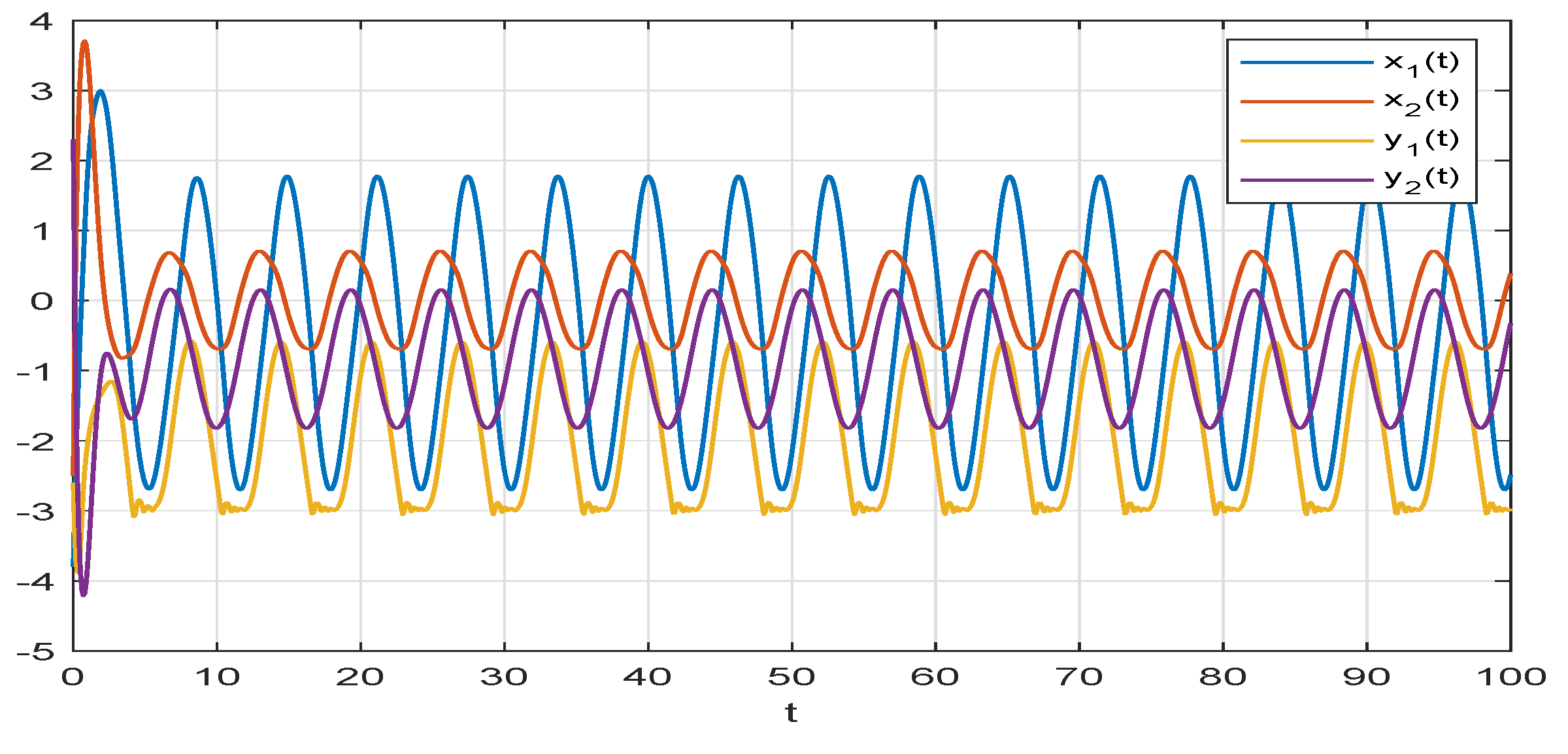
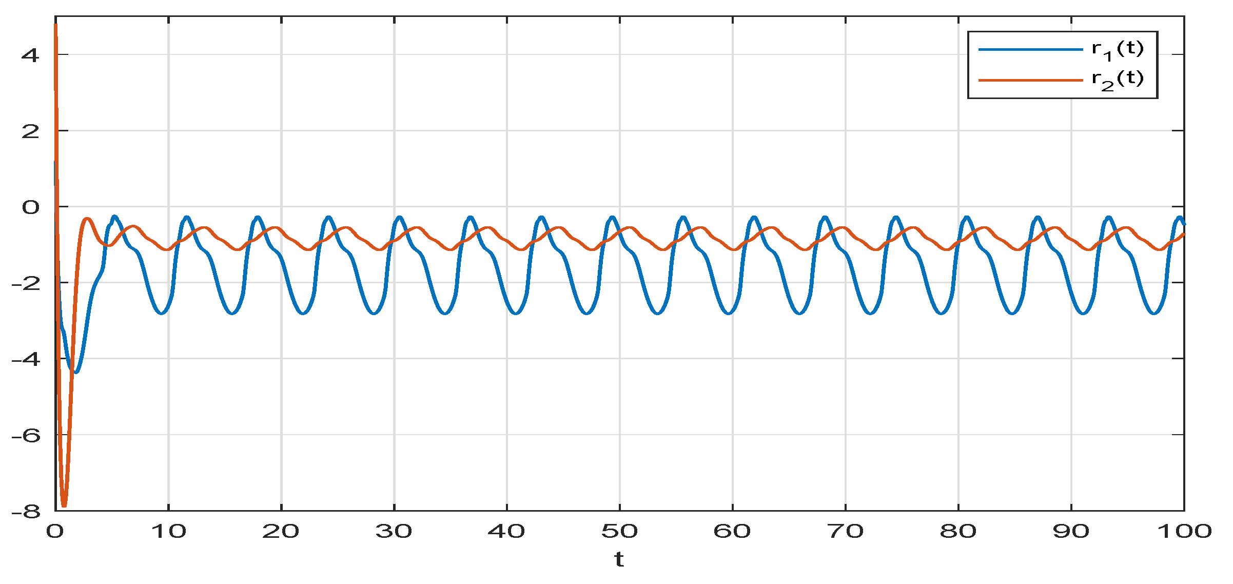
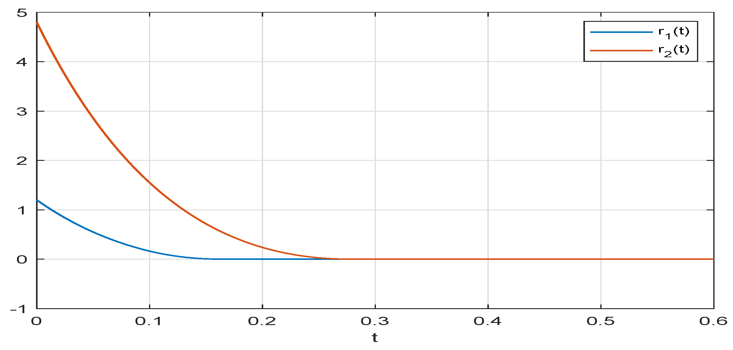
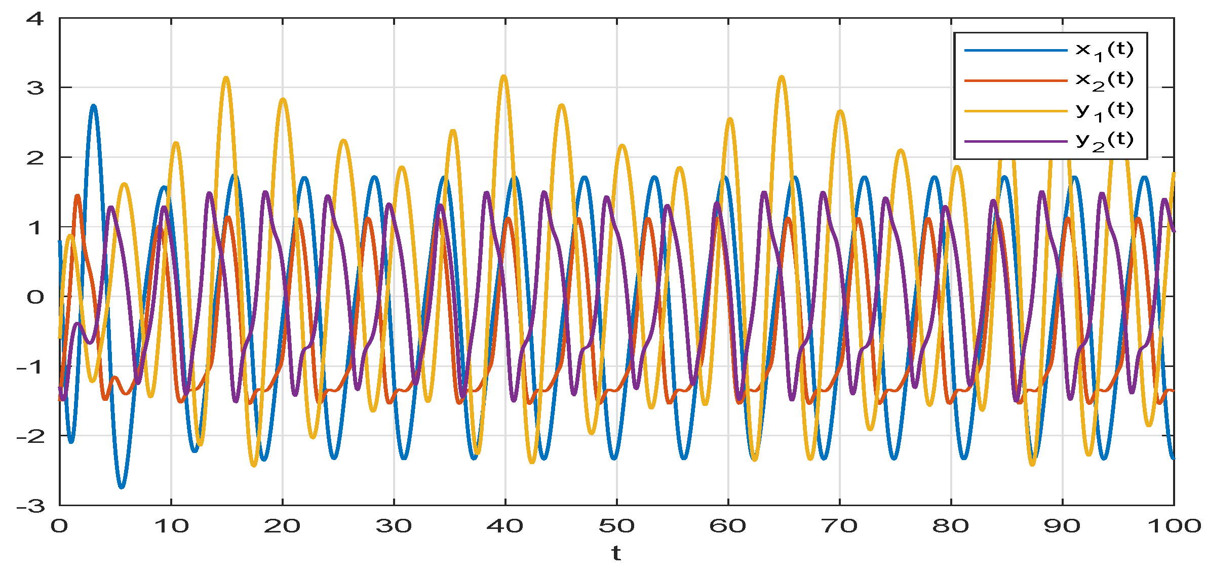
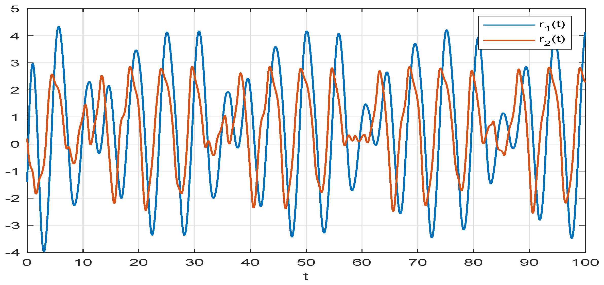
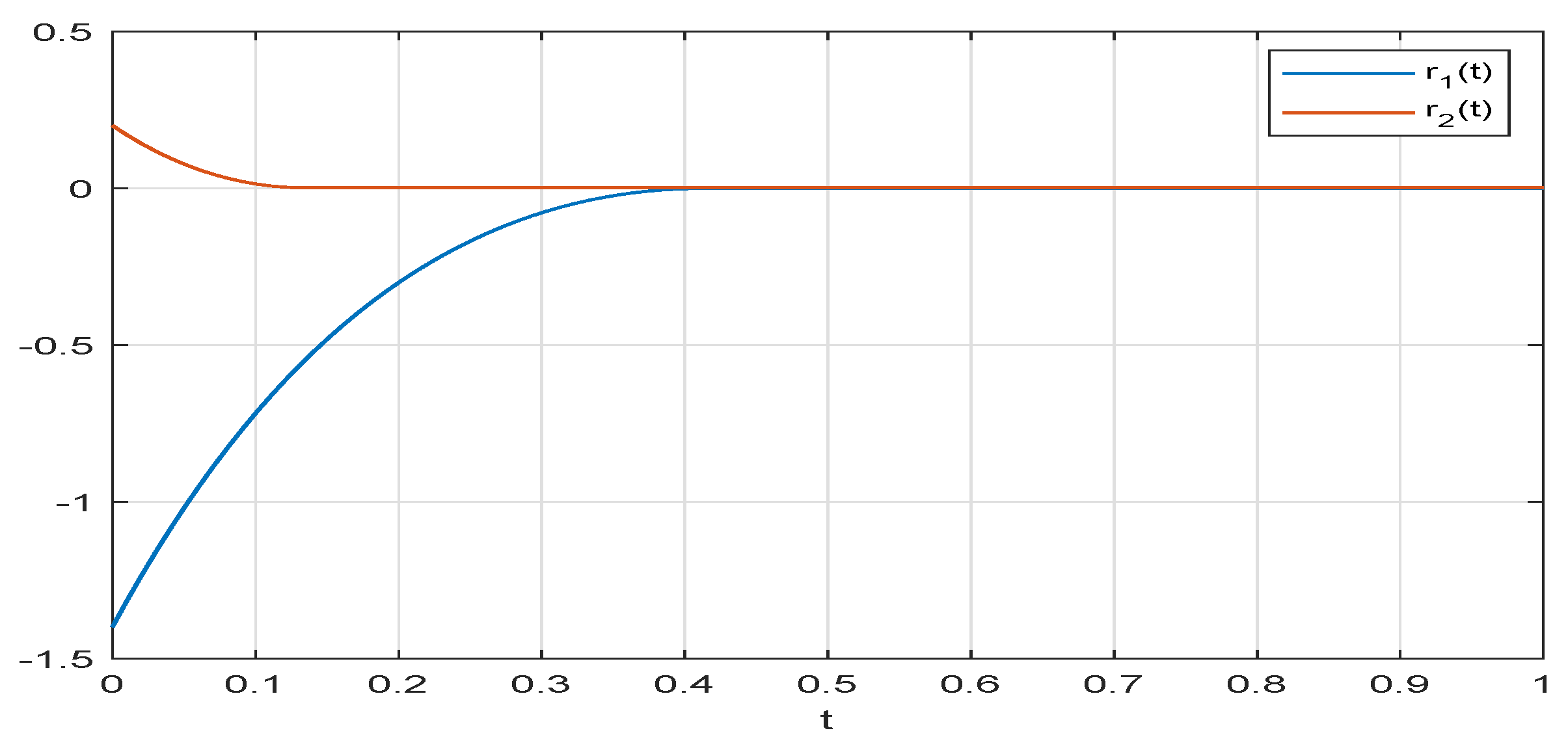
4. Illustrative Example

Example 1.

Consider the two-neuron drive MINNs with MTVDs, as follows:

$$\begin{array}{cc}\hfill \frac{d^2{x}_i\left(t\right)}{d{t}^2}=& -a_i\frac{d{x}_i\left(t\right)}{dt}-b_i{x}_i\left(t\right)+\sum _{j=1}^2{c}_{ij}\left(x_i\left(t\right)\right)f_j\left(x_j\left(t\right)\right)+\sum _{j=1}^2{d}_{ij}\left(x_i\left(t\right)\right)\hfill \\ \hfill & \times f_j\left(x_j(t-\tau \left(t\right))\right)+\sum _{j=1}^2{e}_{ij}\left(x_i\left(t\right)\right){\int }_{t-\ell \left(t\right)}^t{f}_j\left(x_j\left(s\right)\right)ds+I_i\left(t\right)\hfill \end{array}$$

(14)

$i=1,2,$ where $a_1=2.52,$ $a_2=3.14,$ $b_1=3.39,$ $b_2=3.78,$ and the activation functions $f_1(·)=f_2(·)=tanh(·),$ $\tau \left(t\right)=\ell \left(t\right)=\frac{e^t}{1+e^t},$ $I_1\left(t\right)=5sin\left(t\right),$ $I_2\left(t\right)=5cos\left(t\right).$ We can clearly observe that the functions $f_1$ and $f_2$ satisfy Assumption 1 and 2 with $l_1=l_2=1,$ $M_1=M_2=1,$ and $0\le \tau \left(t\right),\ell \left(t\right)\le 1.$ The memristor-based connection weights take the following forms:

$$\begin{array}{cc}\hfill & c_{11}\left(x_1\left(t\right)\right)=\left\{\begin{array}{c}5.21,|x_1\left(t\right)|\le T_1,\hfill \\ -3.48,|x_1\left(t\right)|>T_1,\hfill \end{array}\right.c_{12}\left(x_1\left(t\right)\right)=\left\{\begin{array}{c}4.25,|x_1\left(t\right)|\le T_1,\hfill \\ -5.37,|x_1\left(t\right)|>T_1,\hfill \end{array}\right.\hfill \\ \hfill & c_{21}\left(x_2\left(t\right)\right)=\left\{\begin{array}{c}3.37,|x_2\left(t\right)|\le T_2,\hfill \\ 2.62,|x_2\left(t\right)|>T_2,\hfill \end{array}\right.c_{22}\left(x_2\left(t\right)\right)=\left\{\begin{array}{c}-4.63,|x_2\left(t\right)|\le T_2,\hfill \\ 3.77,|x_2\left(t\right)|>T_2,\hfill \end{array}\right.\hfill \\ \hfill & d_{11}\left(x_1\left(t\right)\right)=\left\{\begin{array}{c}2.59,|x_1\left(t\right)|\le T_1,\hfill \\ -5.47,|x_1\left(t\right)|>T_1,\hfill \end{array}\right.d_{12}\left(x_1\left(t\right)\right)=\left\{\begin{array}{c}-3.56,|x_1\left(t\right)|\le T_1,\hfill \\ -4.28,|x_1\left(t\right)|>T_1,\hfill \end{array}\right.\hfill \\ \hfill & d_{21}\left(x_2\left(t\right)\right)=\left\{\begin{array}{c}2.07,|x_2\left(t\right)|\le T_2,\hfill \\ 3.69,|x_2\left(t\right)|>T_2,\hfill \end{array}\right.d_{22}\left(x_2\left(t\right)\right)=\left\{\begin{array}{c}-4.37,|x_2\left(t\right)|\le T_2,\hfill \\ 4.92,|x_2\left(t\right)|>T_2,\hfill \end{array}\right.\hfill \\ \hfill & e_{11}\left(x_1\left(t\right)\right)=\left\{\begin{array}{c}-4.36,|x_1\left(t\right)|\le T_1,\hfill \\ 2.55,|x_1\left(t\right)|>T_1,\hfill \end{array}\right.e_{12}\left(x_1\left(t\right)\right)=\left\{\begin{array}{c}2.33,|x_1\left(t\right)|\le T_1,\hfill \\ 5.47,|x_1\left(t\right)|>T_1,\hfill \end{array}\right.\hfill \\ \hfill & e_{21}\left(x_2\left(t\right)\right)=\left\{\begin{array}{c}-3.78,|x_2\left(t\right)|\le T_2,\hfill \\ 5.64,|x_2\left(t\right)|>T_2,\hfill \end{array}\right.e_{22}\left(x_2\left(t\right)\right)=\left\{\begin{array}{c}4.39,|x_2\left(t\right)|\le T_2,\hfill \\ 5.24,|x_2\left(t\right)|>T_2.\hfill \end{array}\right.\hfill \end{array}$$

where $T_1=3,$ $T_2=10.$ The initial value of system (14) are $x_1\left(0\right)=-3.8,$ $x_1^{\prime }\left(0\right)=7.8,$ $x_2\left(0\right)=-2.5,$ $x_2^{\prime }\left(0\right)=22.3.$ The corresponding response MINNs as follows:

$$\begin{array}{cc}\hfill \frac{d^2{y}_i\left(t\right)}{d{t}^2}=& -a_i\frac{d{y}_i\left(t\right)}{dt}-b_i{y}_i\left(t\right)+\sum _{j=1}^2{c}_{ij}\left(y_i\left(t\right)\right)f_j\left(y_j\left(t\right)\right)+\sum _{j=1}^2{d}_{ij}\left(y_i\left(t\right)\right)\hfill \\ \hfill & \times f_j\left(y_j(t-\tau \left(t\right))\right)+\sum _{j=1}^2{e}_{ij}\left(y_i\left(t\right)\right){\int }_{t-\ell \left(t\right)}^t{f}_j\left(y_j\left(s\right)\right)ds+I_i\left(t\right)+U_i\left(t\right)\hfill \end{array}$$

(15)

where $i=1,2,$ the initial value of system (15) are $y_1\left(0\right)=-2.6,$ $y_1^{\prime }\left(0\right)=-8.35,$ $y_2\left(0\right)=2.3,$ $y_2^{\prime }\left(0\right)=-24.4,$ and the controllers $U_i\left(t\right)$ are defined in (7). The drive and response MINNs (14) and (15) and their synchronization error system without controller are given in Figure 2 and Figure 3, which imply that drive-response MINNs will not achieve synchronization as time increases.

Obviously, we can obtain that $1-a_1=-1.52,1-a_2=-2.14,$ ${\displaystyle b_1+l_1\sum _{j=1}^2{\overline{c}}_{j1}=11.97,}$ ${\displaystyle b_2+l_2\sum _{j=1}^2{\overline{c}}_{j2}=13.78,}$ and $\left|\right|(\widehat{C}-\breve{C})M|{|}_1=32.70,$ $\left|\right|(\widehat{D}-\breve{D})M|{|}_1=30.95,$ $\ell \left|\right|(\widehat{E}-\breve{E})M|{|}_1=33.76,$ so we have $\left|\right|\beta |{|}_1>97.41.$ Choose ${\lambda }_1={\lambda }_2=1,$ ${\theta }_1={\theta }_2=15,$ ${\beta }_1={\beta }_2=50,$ $\xi =1.5$ and $\mu =0.8,$ then the condition in Theorem 1 or Theorem 2 is satisfied. According to Theorem 1 or Theorem 2, the drive MINNs (14) and the response MINNS (15) can achieve FTS with the controller (14), and the estimated value of settling time $T\le 7.77$ or $T\le 4.36.$ Figure 4 shows the synchronization error trajectories of drive-response MINNs (14) and (15) under the controller (7). The drive-response MINNs are successfully synchronized in the finite time. Therefore, the correctness of Theorems 1 and 2 is certified.

Example 2.

Consider the two-neuron drive MINNs with MTVDs, as follows:

$$\begin{array}{cc}\hfill \frac{d^2{x}_i\left(t\right)}{d{t}^2}=& -a_i\frac{d{x}_i\left(t\right)}{dt}-b_i{x}_i\left(t\right)+\sum _{j=1}^2{c}_{ij}\left(x_i\left(t\right)\right)f_j\left(x_j\left(t\right)\right)+\sum _{j=1}^2{d}_{ij}\left(x_i\left(t\right)\right)\hfill \\ \hfill & \times f_j\left(x_j(t-\tau \left(t\right))\right)+\sum _{j=1}^2{e}_{ij}\left(x_i\left(t\right)\right){\int }_{t-\ell \left(t\right)}^t{f}_j\left(x_j\left(s\right)\right)ds+I_i\left(t\right)\hfill \end{array}$$

(16)

$i=1,2,$ where $a_1=1.32,$ $a_2=1.43,$ $b_1=1.57,$ $b_2=1.33,$ and the activation functions $f_1(·)=f_2(·)=tanh(·),$ $\tau \left(t\right)=\ell \left(t\right)=\frac{e^t}{1+e^t},$ $I_1\left(t\right)=sin\left(t\right),$ $I_2\left(t\right)=cos\left(t\right).$ We can clearly observe that the functions $f_1$ and $f_2$ satisfy Assumption 1 and 2 with $l_1=l_2=1,$ $M_1=M_2=1,$ and $0\le \tau \left(t\right),\ell \left(t\right)\le 1.$ The memristor-based connection weights take the following forms:

$$\begin{array}{cc}\hfill & c_{11}\left(x_1\left(t\right)\right)=\left\{\begin{array}{c}1.15,|x_1\left(t\right)|\le T_1,\hfill \\ -1.34,|x_1\left(t\right)|>T_1,\hfill \end{array}\right.c_{12}\left(x_1\left(t\right)\right)=\left\{\begin{array}{c}1.44,|x_1\left(t\right)|\le T_1,\hfill \\ 1.53,|x_1\left(t\right)|>T_1,\hfill \end{array}\right.\hfill \\ \hfill & c_{21}\left(x_2\left(t\right)\right)=\left\{\begin{array}{c}-1.83,|x_2\left(t\right)|\le T_2,\hfill \\ 1.47,|x_2\left(t\right)|>T_2,\hfill \end{array}\right.c_{22}\left(x_2\left(t\right)\right)=\left\{\begin{array}{c}1.28,|x_2\left(t\right)|\le T_2,\hfill \\ -1.66,|x_2\left(t\right)|>T_2,\hfill \end{array}\right.\hfill \\ \hfill & d_{11}\left(x_1\left(t\right)\right)=\left\{\begin{array}{c}-1.73,|x_1\left(t\right)|\le T_1,\hfill \\ -1.48,|x_1\left(t\right)|>T_1,\hfill \end{array}\right.d_{12}\left(x_1\left(t\right)\right)=\left\{\begin{array}{c}1.27,|x_1\left(t\right)|\le T_1,\hfill \\ -1.19,|x_1\left(t\right)|>T_1,\hfill \end{array}\right.\hfill \\ \hfill & d_{21}\left(x_2\left(t\right)\right)=\left\{\begin{array}{c}-1.63,|x_2\left(t\right)|\le T_2,\hfill \\ -1.38,|x_2\left(t\right)|>T_2,\hfill \end{array}\right.d_{22}\left(x_2\left(t\right)\right)=\left\{\begin{array}{c}-1.55,|x_2\left(t\right)|\le T_2,\hfill \\ 1.82,|x_2\left(t\right)|>T_2,\hfill \end{array}\right.\hfill \\ \hfill & e_{11}\left(x_1\left(t\right)\right)=\left\{\begin{array}{c}-1.14,|x_1\left(t\right)|\le T_1,\hfill \\ 1.52,|x_1\left(t\right)|>T_1,\hfill \end{array}\right.e_{12}\left(x_1\left(t\right)\right)=\left\{\begin{array}{c}1.57,|x_1\left(t\right)|\le T_1,\hfill \\ 1.46,|x_1\left(t\right)|>T_1,\hfill \end{array}\right.\hfill \\ \hfill & e_{21}\left(x_2\left(t\right)\right)=\left\{\begin{array}{c}-1.35,|x_2\left(t\right)|\le T_2,\hfill \\ 1.86,|x_2\left(t\right)|>T_2,\hfill \end{array}\right.e_{22}\left(x_2\left(t\right)\right)=\left\{\begin{array}{c}1.74,|x_2\left(t\right)|\le T_2,\hfill \\ -1.58,|x_2\left(t\right)|>T_2.\hfill \end{array}\right.\hfill \end{array}$$

where $T_1=1,$ $T_2=1.$ The initial value of system (16) are $x_1\left(0\right)=0.8,$ $x_1^{\prime }\left(0\right)=-4.8,$ $x_2\left(0\right)=-1.5,$ $x_2^{\prime }\left(0\right)=1.8.$ The corresponding response MINNs are as follows:

$$\begin{array}{cc}\hfill \frac{d^2{y}_i\left(t\right)}{d{t}^2}=& -a_i\frac{d{y}_i\left(t\right)}{dt}-b_i{y}_i\left(t\right)+\sum _{j=1}^2{c}_{ij}\left(y_i\left(t\right)\right)f_j\left(y_j\left(t\right)\right)+\sum _{j=1}^2{d}_{ij}\left(y_i\left(t\right)\right)\hfill \\ \hfill & \times f_j\left(y_j(t-\tau \left(t\right))\right)+\sum _{j=1}^2{e}_{ij}\left(y_i\left(t\right)\right){\int }_{t-\ell \left(t\right)}^t{f}_j\left(y_j\left(s\right)\right)ds+I_i\left(t\right)+U_i\left(t\right)\hfill \end{array}$$

(17)

where $i=1,2,$ the initial value of system (17) are $y_1\left(0\right)=-0.6,$ $y_1^{\prime }\left(0\right)=3.65,$ $y_2\left(0\right)=-1.3,$ $y_2^{\prime }\left(0\right)=-1.3,$ and the controllers $U_i\left(t\right)$ are defined in (10). When the controllers $U_i\left(t\right)=0,$ the drive and response MINNs (16) and (17) and its synchronization error system are given in Figure 5 and Figure 6, which imply that drive-response MINNs will not achieve synchronization as time increases.

According to Theorem 3, we can obtain that $1-a_1=-0.32,1-a_2=-0.43,$ ${\displaystyle b_1+l_1\sum _{j=1}^2{\overline{c}}_{j1}=4.74,}$ ${\displaystyle b_2+l_2\sum _{j=1}^2{\overline{c}}_{j2}=4.52,}$ and $\left|\right|(\widehat{C}-\breve{C})M|{|}_1=8.82,$ $\left|\right|(\widehat{D}-\breve{D})M|{|}_1=6.33,$ $\ell \left|\right|(\widehat{E}-\breve{E})M|{|}_1=9.30,$; thus, we have $\left|\right|\beta |{|}_1>24.45.$ Then, choose ${\lambda }_1={\lambda }_2=1,$ ${\theta }_1={\theta }_2=5,$ and ${\beta }_1=10,{\beta }_2=16,$; the error systems with the controller are shown in Figure 7,and the settling time $T\le 4.48.$ It is easy to observe from Figure 7 that the drive-response MINNs (16) and (17) are successfully synchronization in the finite time with the controller (10); thus, the practicality and validity of Theorem 3 are shown.

5. Conclusions

In this work, novel sufficient conditions to guarantee the FTS for the studied MINNs have been given. Moreover, the novel finite-time stability criterion proposed in this paper is completely different from the existing ones, and it enriches the analytical tools for studying FTS. In addition, we directly investigated the FTS from the MINNs themselves without utilizing the variable substitution method widely used in the previous literature, which does not change the order of the second-order MINNs. Finally, several numerical examples have also been provided to demonstrate the validity of the novel research results. New useful study methods and theoretical results of this paper have widened the existing results, and this can be extended to many dynamical systems, such as nonlinear impulsive systems, and coupled neural networks, which are our possible future research topics.

References

1. Chong, E.K.P.; Hui, S.; Zak, S.H. An analysis of a class of neural networks for solving linear programming problems. IEEE Trans. Autom. Control 1999, 44, 1995–2006. [Google Scholar] [CrossRef]
2. Lee, T.H.; Trinh, H.M.; Park, J.H. Stability Analysis of Neural Networks with Time-Varying Delay by Constructing Novel Lyapunov Functionals. IEEE Trans. Neural Netw. Learn. Syst. 2018, 29, 4238–4247. [Google Scholar] [CrossRef]
3. Chen, J.; Park, J.H.; Xu, S. Stability Analysis for Neural Networks with Time-Varying Delay via Improved Techniques. IEEE Trans. Cybern. 2019, 49, 4495–4500. [Google Scholar] [CrossRef] [PubMed]
4. Zhang, C.; He, Y.; Jiang, L.; Wu, M. Stability Analysis for Delayed Neural Networks Considering Both Conservativeness and Complexity. IEEE Trans. Neural Netw. Learn. Syst. 2016, 27, 1486–1501. [Google Scholar] [CrossRef] [PubMed] [Green Version]
5. Dong, S.; Zhong, S.; Shi, K.; Kang, W.; Cheng, J. Further improved results on non-fragile H performance state estimation for delayed static neural networks. Neurocomputing 2019, 356, 9–20. [Google Scholar] [CrossRef]
6. Kiannejad, M.; Salehizadeh, M.R.; Oloomi-Buygi, M.; Baringo, L. A stochastic offering approach for photovoltaic power plants in day-ahead and balancing markets. Int. J. Electr. Power Energy Syst. 2023, 147, 108841. [Google Scholar] [CrossRef]
7. Kiannejad, M.; Salehizadeh, M.R.; Oloomi-Buygi, M. Two-stage ANN-based bidding strategy for a load aggregator using decentralized equivalent rival concept. IET Gener. Transm. Distrib. 2021, 15, 56–70. [Google Scholar] [CrossRef]
8. Chen, J.; Zeng, Z.; Jiang, P. Global Mittag-Leffler stability and synchronization of memristor-based fractional-order neural networks. Neural Netw. 2014, 51, 1–8. [Google Scholar] [CrossRef]
9. Hua, L.; Zhong, S.; Shi, K.; Zhang, X. Further results on finite-time synchronization of delayed inertial memristive neural networks via a novel analysis method. Neural Netw. 2020, 127, 47–57. [Google Scholar] [CrossRef]
10. Bao, H.; Park, J.H.; Cao, J. Adaptive synchronization of fractional-order memristor-based neural networks with time delay. Nonlinear Dyn. 2015, 82, 1343–1354. [Google Scholar] [CrossRef]
11. Liu, Y.; Tong, L.; Lou, J.; Lu, J.; Cao, J. Sampled-Data Control for the Synchronization of Boolean Control Networks. IEEE Trans. Cybern. 2019, 49, 726–732. [Google Scholar] [CrossRef] [PubMed]
12. Hua, L.; Zhu, H.; Shi, K.; Zhong, S.; Tang, Y.; Liu, Y. Novel Finite-Time Reliable Control Design for Memristor-Based Inertial Neural Networks with Mixed Time-Varying Delays. IEEE Trans. Circuits Syst. I Regul. Pap. 2021, 68, 1599–1609. [Google Scholar] [CrossRef]
13. Zhang, R.; Park, J.H.; Zeng, D.; Liu, Y.; Zhong, S. A new method for exponential synchronization of memristive recurrent neural networks. Inf. Sci. 2018, 466, 152–169. [Google Scholar] [CrossRef]
14. Zhang, G.; Zeng, Z.; Ning, D. Novel results on synchronization for a class of switched inertial neural networks with distributed delays. Inf. Sci. 2020, 511, 114–126. [Google Scholar] [CrossRef]
15. Zhang, R.; Zeng, D.; Park, J.H.; Liu, Y.; Zhong, S. Quantized Sampled-Data Control for Synchronization of Inertial Neural Networks with Heterogeneous Time-Varying Delays. IEEE Trans. Neural Netw. Learn. Syst. 2018, 29, 6385–6395. [Google Scholar] [CrossRef] [PubMed]
16. Guan, C.; Fei, Z.; Karimi, H.R.; Shi, P. Finite-Time Synchronization for Switched Neural Networks via Quantized Feedback Control. IEEE Trans. Syst. Man Cybern. Syst. 2021, 51, 2873–2884. [Google Scholar] [CrossRef]
17. Zhang, Z.; Cao, J. Novel Finite-Time Synchronization Criteria for Inertial Neural Networks with Time Delays via Integral Inequality Method. IEEE Trans. Neural Netw. Learn. Syst. 2019, 30, 1476–1485. [Google Scholar] [CrossRef]
18. Alimi, A.M.; Aouiti, C.; Assali, E.A. Finite-time and fixed-time synchronization of a class of inertial neural networks with multi-proportional delays and its application to secure communication. Neurocomputing 2019, 332, 29–43. [Google Scholar] [CrossRef]
19. Hua, L.; Zhu, H.; Zhong, S.; Zhang, Y.; Shi, K.; Kwon, O.M. Fixed-Time Stability of Nonlinear Impulsive Systems and Its Application to Inertial Neural Networks. IEEE Trans. Neural Netw. Learn. Syst. 2022, 1–12. [Google Scholar] [CrossRef]
20. Babcock, K.; Westervelt, R. Stability and dynamics of simple electronic neural networks with added inertia. Phys. D Nonlinear Phenom. 1986, 23, 464–469. [Google Scholar] [CrossRef]
21. Babcock, K.; Westervelt, R. Dynamics of simple electronic neural networks. Phys. D Nonlinear Phenom. 1987, 28, 305–316. [Google Scholar] [CrossRef]
22. Wheeler, D.W.; Schieve, W. Stability and chaos in an inertial two-neuron system. Phys. D Nonlinear Phenom. 1997, 105, 267–284. [Google Scholar] [CrossRef]
23. Angelaki, D.E.; Correia, M.J. Models of membrane resonance in pigeon semicircular canal type II hair cells. Biol. Cybern. 1991, 65, 1–10. [Google Scholar] [CrossRef]
24. Tani, J. Model-based learning for mobile robot navigation from the dynamical systems perspective. IEEE Trans. Syst. Man Cybern. Part B (Cybern.) 1996, 26, 421–436. [Google Scholar] [CrossRef] [PubMed] [Green Version]
25. Yunquan, K.; Chunfang, M. Stability and existence of periodic solutions in inertial BAM neural networks with time delay. Neural Comput. Appl. 2013, 23, 1089–1099. [Google Scholar] [CrossRef]
26. Xiao, Q.; Huang, T.; Zeng, Z. Global Exponential Stability and Synchronization for Discrete-Time Inertial Neural Networks with Time Delays: A Timescale Approach. IEEE Trans. Neural Netw. Learn. Syst. 2019, 30, 1854–1866. [Google Scholar] [CrossRef] [PubMed]
27. Li, N.; Zheng, W.X. Synchronization criteria for inertial memristor-based neural networks with linear coupling. Neural Netw. 2018, 106, 260–270. [Google Scholar] [CrossRef]
28. Zhang, G.; Zeng, Z. Stabilization of Second-Order Memristive Neural Networks with Mixed Time Delays via Nonreduced Order. IEEE Trans. Neural Netw. Learn. Syst. 2020, 31, 700–706. [Google Scholar] [CrossRef]
29. Zhang, G.; Zeng, Z.; Hu, J. New results on global exponential dissipativity analysis of memristive inertial neural networks with distributed time-varying delays. Neural Netw. 2018, 97, 183–191. [Google Scholar] [CrossRef]
30. Lakshmanan, S.; Prakash, M.; Lim, C.P.; Rakkiyappan, R.; Balasubramaniam, P.; Nahavandi, S. Synchronization of an Inertial Neural Network with Time-Varying Delays and Its Application to Secure Communication. IEEE Trans. Neural Netw. Learn. Syst. 2018, 29, 195–207. [Google Scholar] [CrossRef]
31. Xu, C.; Zhang, Q. Existence and global exponential stability of anti-periodic solutions for BAM neural networks with inertial term and delay. Neurocomputing 2015, 153, 108–116. [Google Scholar] [CrossRef]
32. Prakash, M.; Balasubramaniam, P.; Lakshmanan, S. Synchronization of Markovian jumping inertial neural networks and its applications in image encryption. Neural Netw. 2016, 83, 86–93. [Google Scholar] [CrossRef] [PubMed]
33. Wang, Q.; Perc, M.; Duan, Z.; Chen, G. Impact of delays and rewiring on the dynamics of small-world neuronal networks with two types of coupling. Phys. A Stat. Mech. Its Appl. 2010, 389, 3299–3306. [Google Scholar] [CrossRef]
34. Wang, Q.; Chen, G.; Perc, M. Synchronous Bursts on Scale-Free Neuronal Networks with Attractive and Repulsive Coupling. PLoS ONE 2011, 6, e15851. [Google Scholar] [CrossRef] [PubMed] [Green Version]
35. Guo, D.; Wang, Q.; Perc, M. Complex synchronous behavior in interneuronal networks with delayed inhibitory and fast electrical synapses. Phys. Rev. E 2012, 85, 061905. [Google Scholar] [CrossRef] [PubMed] [Green Version]
36. Strukov, D.B.; Snider, G.S.; Stewart, D.R.; Williams, R.S. The missing memristor found. Nature 2008, 453, 80–83. [Google Scholar] [CrossRef]
37. Jo, S.H.; Chang, T.; Ebong, I.; Bhadviya, B.B.; Mazumder, P.; Lu, W. Nanoscale memristor device as synapse in neuromorphic systems. Nano Lett. 2010, 10, 1297–1301. [Google Scholar] [CrossRef]
38. Corinto, F.; Forti, M. Memristor Circuits: Flux–Charge Analysis Method. IEEE Trans. Circuits Syst. I Regul. Pap. 2016, 63, 1997–2009. [Google Scholar] [CrossRef] [Green Version]
39. Kim, H.; Sah, M.P.; Yang, C.; Roska, T.; Chua, L.O. Neural Synaptic Weighting with a Pulse-Based Memristor Circuit. IEEE Trans. Circuits Syst. I Regul. Pap. 2012, 59, 148–158. [Google Scholar] [CrossRef]
40. Duan, S.; Hu, X.; Dong, Z.; Wang, L.; Mazumder, P. Memristor-Based Cellular Nonlinear/Neural Network: Design, Analysis, and Applications. IEEE Trans. Neural Netw. Learn. Syst. 2015, 26, 1202–1213. [Google Scholar] [CrossRef] [PubMed]
41. Zhang, G.; Hu, J.; Zeng, Z. New Criteria on Global Stabilization of Delayed Memristive Neural Networks with Inertial Item. IEEE Trans. Cybern. 2020, 50, 2770–2780. [Google Scholar] [CrossRef] [PubMed]
42. Sheng, Y.; Huang, T.; Zeng, Z.; Li, P. Exponential Stabilization of Inertial Memristive Neural Networks with Multiple Time Delays. IEEE Trans. Cybern. 2021, 51, 579–588. [Google Scholar] [CrossRef] [PubMed]
43. Gong, S.; Yang, S.; Guo, Z.; Huang, T. Global exponential synchronization of inertial memristive neural networks with time-varying delay via nonlinear controller. Neural Netw. 2018, 102, 138–148. [Google Scholar] [CrossRef] [PubMed]
44. Guo, Z.; Gong, S.; Huang, T. Finite-time synchronization of inertial memristive neural networks with time delay via delay-dependent control. Neurocomputing 2018, 293, 100–107. [Google Scholar] [CrossRef]
45. Huang, D.; Jiang, M.; Jian, J. Finite-time synchronization of inertial memristive neural networks with time-varying delays via sampled-date control. Neurocomputing 2017, 266, 527–539. [Google Scholar] [CrossRef]
46. Wei, R.; Cao, J.; Alsaedi, A. Finite-time and fixed-time synchronization analysis of inertial memristive neural networks with time-varying delays. Cogn. Neurodyn. 2018, 12, 121–134. [Google Scholar] [CrossRef]
47. Tang, Y. Terminal sliding mode control for rigid robots. Automatica 1998, 34, 51–56. [Google Scholar] [CrossRef]
48. Shen, Y.; Huang, Y. Uniformly Observable and Globally Lipschitzian Nonlinear Systems Admit Global Finite-Time Observers. IEEE Trans. Autom. Control 2009, 54, 2621–2625. [Google Scholar] [CrossRef]
49. Forti, M.; Grazzini, M.; Nistri, P.; Pancioni, L. Generalized Lyapunov approach for convergence of neural networks with discontinuous or non-Lipschitz activations. Phys. D Nonlinear Phenom. 2006, 214, 88–99. [Google Scholar] [CrossRef]
Figure 1. System constitution and four fundamental elements.
Mathematics 11 00684 g001
Figure 2. The drive-response MINNs without the controller.
Mathematics 11 00684 g002
Figure 3. The synchronization error system without the controller.
Mathematics 11 00684 g003
Figure 4. The synchronization error system with the controller.
Mathematics 11 00684 g004
Figure 5. The drive-response MINNs without the controller.
Mathematics 11 00684 g005
Figure 6. The synchronization error system without the controller.
Mathematics 11 00684 g006
Figure 7. The synchronization error system with the controller.
Mathematics 11 00684 g007
Disclaimer/Publisher’s Note: The statements, opinions and data contained in all publications are solely those of the individual author(s) and contributor(s) and not of MDPI and/or the editor(s). MDPI and/or the editor(s) disclaim responsibility for any injury to people or property resulting from any ideas, methods, instructions or products referred to in the content.