

A New Alpha Power Cosine-Weibull Model with Applications to Hydrological and Engineering Data


Abstract
:1. Introduction
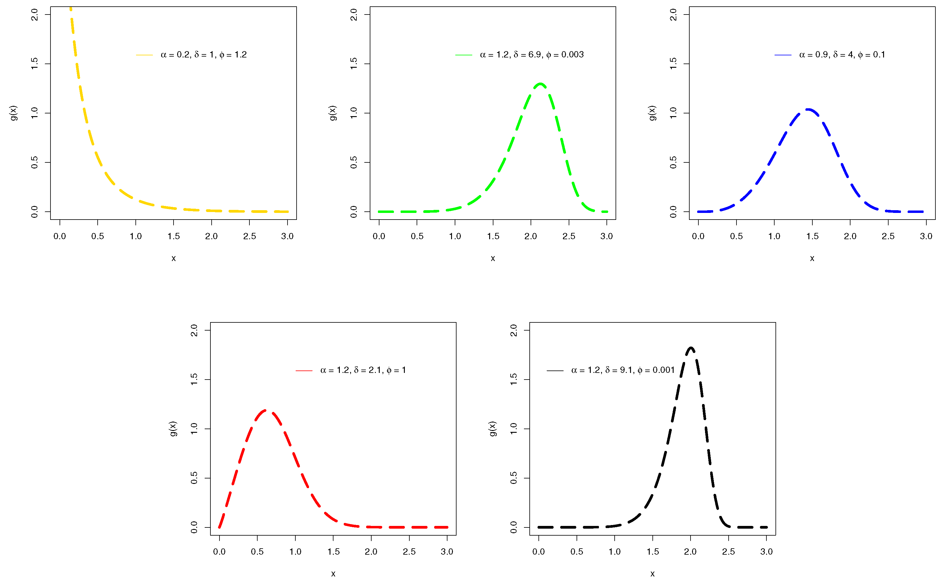
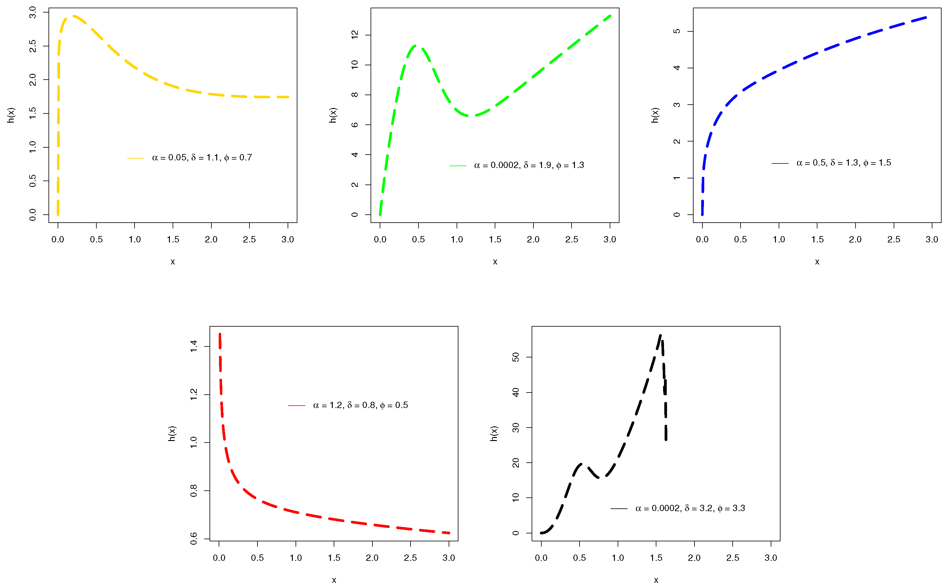
2. A NACos-Weibull Distribution
3. Distributional Properties
3.1. The QF
3.2. The kth Moment
3.3. The MGF
3.4. The CF
4. Estimation and Simulation
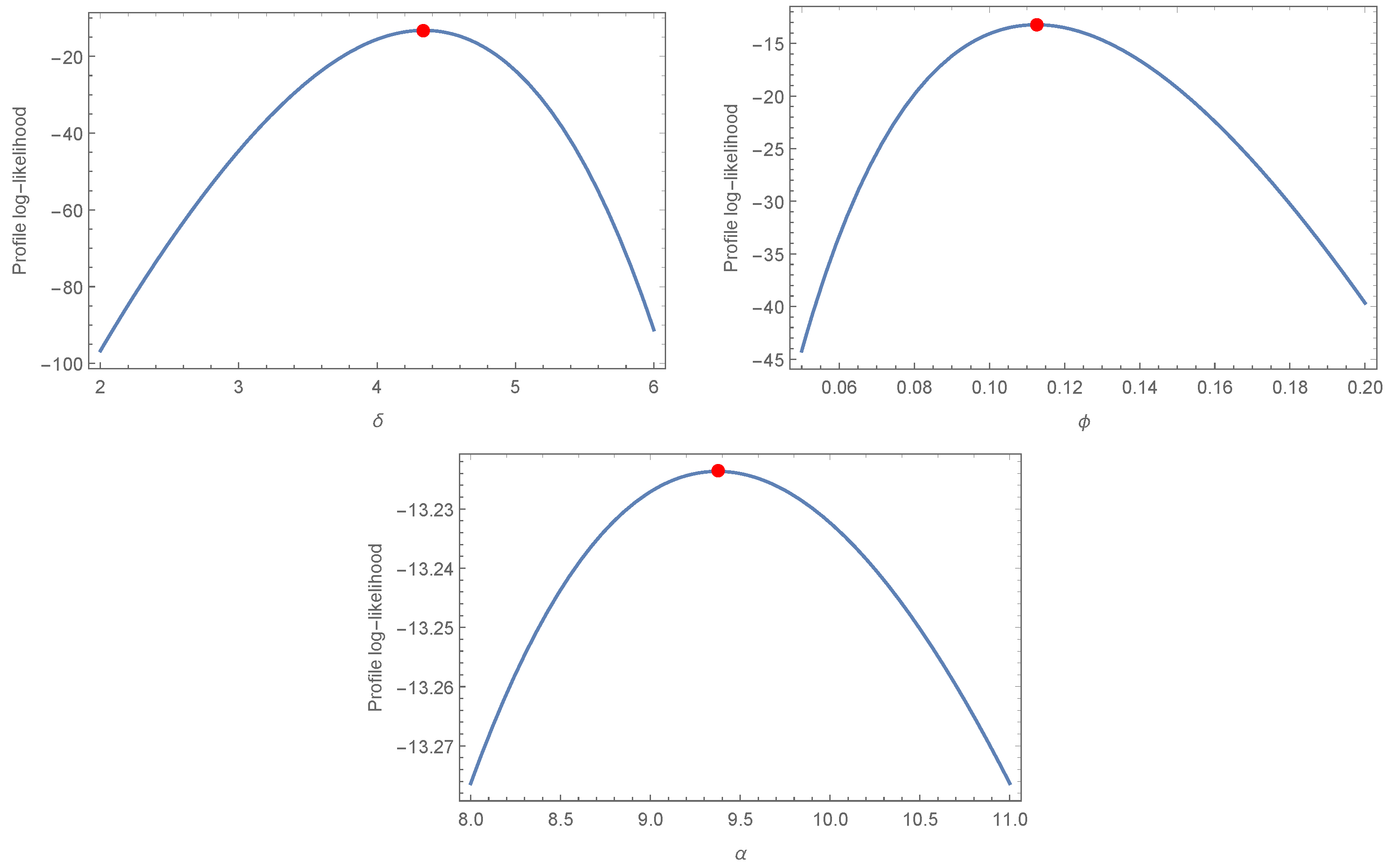
4.1. Estimation
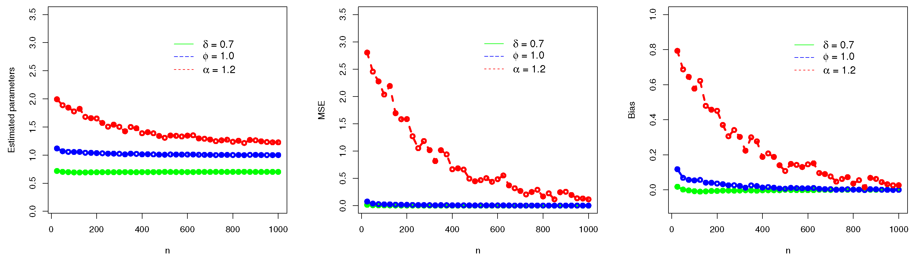
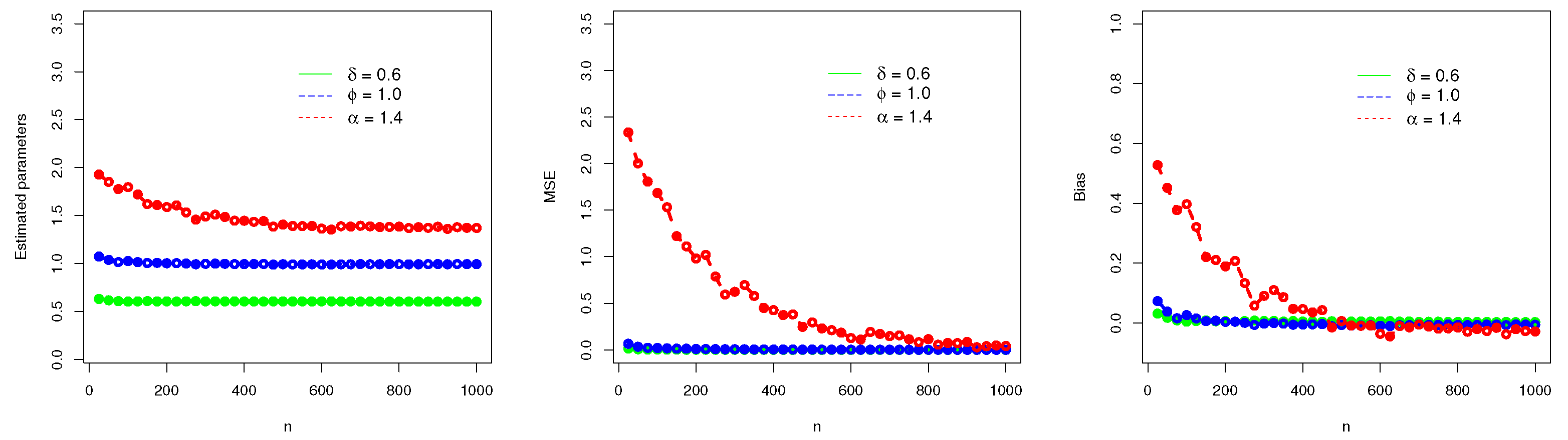
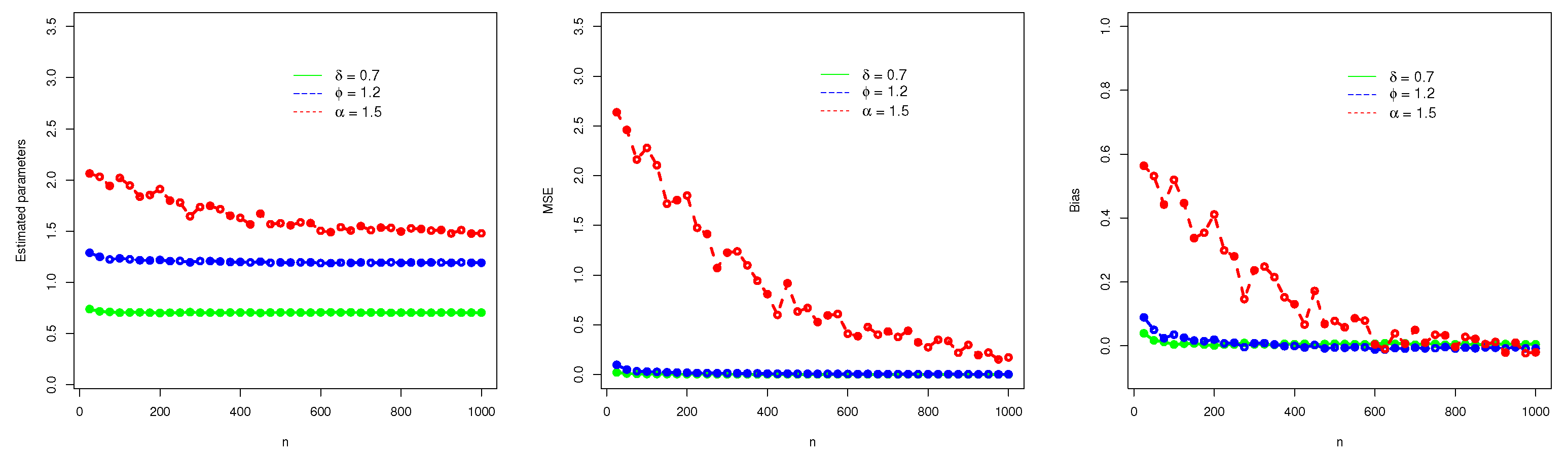
4.2. Simulation
- Mean square error (MSE)
- Bias
- As n increases (i.e., as ), the values of , and tend to become stable.
- As , the MSEs of , and decay to zero.
- As , the Biases of , and tend toward zero.

| n | Parameters | MLEs | MSEs | Biases |
|---|---|---|---|---|
| 0.7179 | 0.0161 | 0.0179 | ||
| 25 | 1.1179 | 0.0761 | 0.1179 | |
| 1.9927 | 2.8029 | 0.7927 | ||
| 0.7020 | 0.0082 | 0.0020 | ||
| 50 | 1.0687 | 0.0382 | 0.0687 | |
| 1.8872 | 2.4542 | 0.6872 | ||
| 0.6968 | 0.0054 | −0.0031 | ||
| 75 | 1.0571 | 0.0277 | 0.0571 | |
| 1.8443 | 2.2757 | 0.6443 | ||
| 0.6927 | 0.0045 | −0.0072 | ||
| 100 | 1.0542 | 0.0249 | 0.0542 | |
| 1.7774 | 2.0346 | 0.5774 | ||
| 0.6939 | 0.0027 | −0.0060 | ||
| 200 | 1.0363 | 0.0162 | 0.0363 | |
| 1.6511 | 1.5851 | 0.4511 | ||
| 0.6978 | 0.0012 | −0.0021 | ||
| 400 | 1.0132 | 0.0070 | 0.0132 | |
| 1.3883 | 0.6674 | 0.1883 | ||
| 0.6983 | 0.0007 | −0.0016 | ||
| 600 | 1.0093 | 0.0051 | 0.0093 | |
| 1.3456 | 0.4851 | 0.1456 | ||
| 0.7016 | 0.0004 | 0.0016 | ||
| 800 | 1.0013 | 0.0025 | 0.0013 | |
| 1.2362 | 0.1696 | 0.0362 | ||
| 0.7009 | 0.0002 | 0.0009 | ||
| 1000 | 1.0002 | 0.0017 | 0.0002 | |
| 1.2267 | 0.1166 | 0.0267 |
| n | Parameters | MLEs | MSEs | Biases |
|---|---|---|---|---|
| 0.6313 | 0.0139 | 0.0313 | ||
| 25 | 1.0730 | 0.0661 | 0.0730 | |
| 1.9276 | 2.3347 | 0.5276 | ||
| 0.6174 | 0.0066 | 0.0174 | ||
| 50 | 1.0380 | 0.0337 | 0.0380 | |
| 1.8515 | 2.0022 | 0.4515 | ||
| 0.6088 | 0.0038 | 0.0088 | ||
| 75 | 1.0157 | 0.0223 | 0.0157 | |
| 1.7771 | 1.8068 | 0.3771 | ||
| 0.6042 | 0.0032 | 0.0042 | ||
| 100 | 1.0261 | 0.0205 | 0.0261 | |
| 1.7970 | 1.6847 | 0.3970 | ||
| 0.6062 | 0.0016 | 0.0062 | ||
| 200 | 1.0036 | 0.0099 | 0.0036 | |
| 1.5894 | 0.9811 | 0.1894 | ||
| 0.6034 | 0.0002 | 0.0034 | ||
| 800 | 0.9935 | 0.0014 | −0.0064 | |
| 1.3848 | 0.1150 | −0.0151 | ||
| 0.6029 | 0.0001 | 0.0029 | ||
| 1000 | 0.9940 | 0.0007 | −0.0059 | |
| 1.3915 | 0.0422 | −0.0284 | ||
| 0.6048 | 0.0007 | 0.0048 | ||
| 400 | 0.9950 | 0.0048 | −0.0049 | |
| 1.4465 | 0.4270 | 0.0465 | ||
| 0.6054 | 0.0003 | 0.0054 | ||
| 600 | 0.9905 | 0.0021 | −0.0094 | |
| 1.3639 | 0.1265 | −0.0360 |
| n | Parameters | MLEs | MSEs | Biases |
|---|---|---|---|---|
| 0.7390 | 0.0209 | 0.0390 | ||
| 25 | 1.2889 | 0.0971 | 0.0889 | |
| 2.0637 | 2.6366 | 0.5637 | ||
| 0.7169 | 0.0098 | 0.0169 | ||
| 50 | 1.2498 | 0.0491 | 0.0498 | |
| 2.0315 | 2.4595 | 0.5315 | ||
| 0.7119 | 0.0062 | 0.0119 | ||
| 75 | 1.2237 | 0.0330 | 0.0237 | |
| 1.9422 | 2.1615 | 0.4422 | ||
| 0.7040 | 0.0047 | 0.0040 | ||
| 100 | 1.2348 | 0.0297 | 0.0348 | |
| 2.0197 | 2.2786 | 0.5197 | ||
| 0.7007 | 0.0031 | 0.0007 | ||
| 200 | 1.2193 | 0.0181 | 0.0193 | |
| 1.9112 | 1.8001 | 0.4112 | ||
| 0.7050 | 0.0014 | 0.0050 | ||
| 400 | 1.1993 | 0.0091 | −0.0006 | |
| 1.6301 | 0.8088 | 0.1301 | ||
| 0.7064 | 0.0009 | 0.0064 | ||
| 600 | 1.1880 | 0.0054 | −0.0119 | |
| 1.5042 | 0.4100 | 0.0042 | ||
| 0.7044 | 0.0006 | 0.0044 | ||
| 800 | 1.1911 | 0.0035 | −0.0088 | |
| 1.4967 | 0.2741 | −0.0032 | ||
| 0.7047 | 0.0004 | 0.0047 | ||
| 1000 | 1.1915 | 0.0026 | −0.0084 | |
| 1.4994 | 0.1718 | −0.0205 |


5. Applications Using the Hydrological and Engineering Data Sets
- The Anderson Darling (represented by AD) testThe AD test is a statistical quantity used to show the fitting power of a particular probability model for the underline data set. The main work of the AD test is to show if a considered sample of data is taken from the target population using a specific statistical model. The AD test can also be considered as an alternative test to the test and computed aswhere w is given by .
- The Cramer-Von-Messes (denoted by CVM) testThe CVM test is another useful evaluating criterion for comparing the fitting power (or fitting results) of two or more probability models. A probability model with the lowest value of the CVM criterion is preferred. The numerical value of the CVM test is obtained as
- The Kolmogorov–Smirnov (expressed by KS) testAnother criterion that we considered for comparing the NACos-Weibull and other competing models is the KS test. Let and represent the fitted CDF (i.e., CDF of the selected model) and empirical CDF, respectively. Then, the value of the KS criterion is computed as
- Akaike information criterion (AIC) The Akaike information criterion (AIC) is another decisive tool for checking how well a particular probability model fits the underlined data set. Let k represent the number of parameters of a model and ℓ represent the corresponding LLF of the model; then, the value of AIC is obtained as
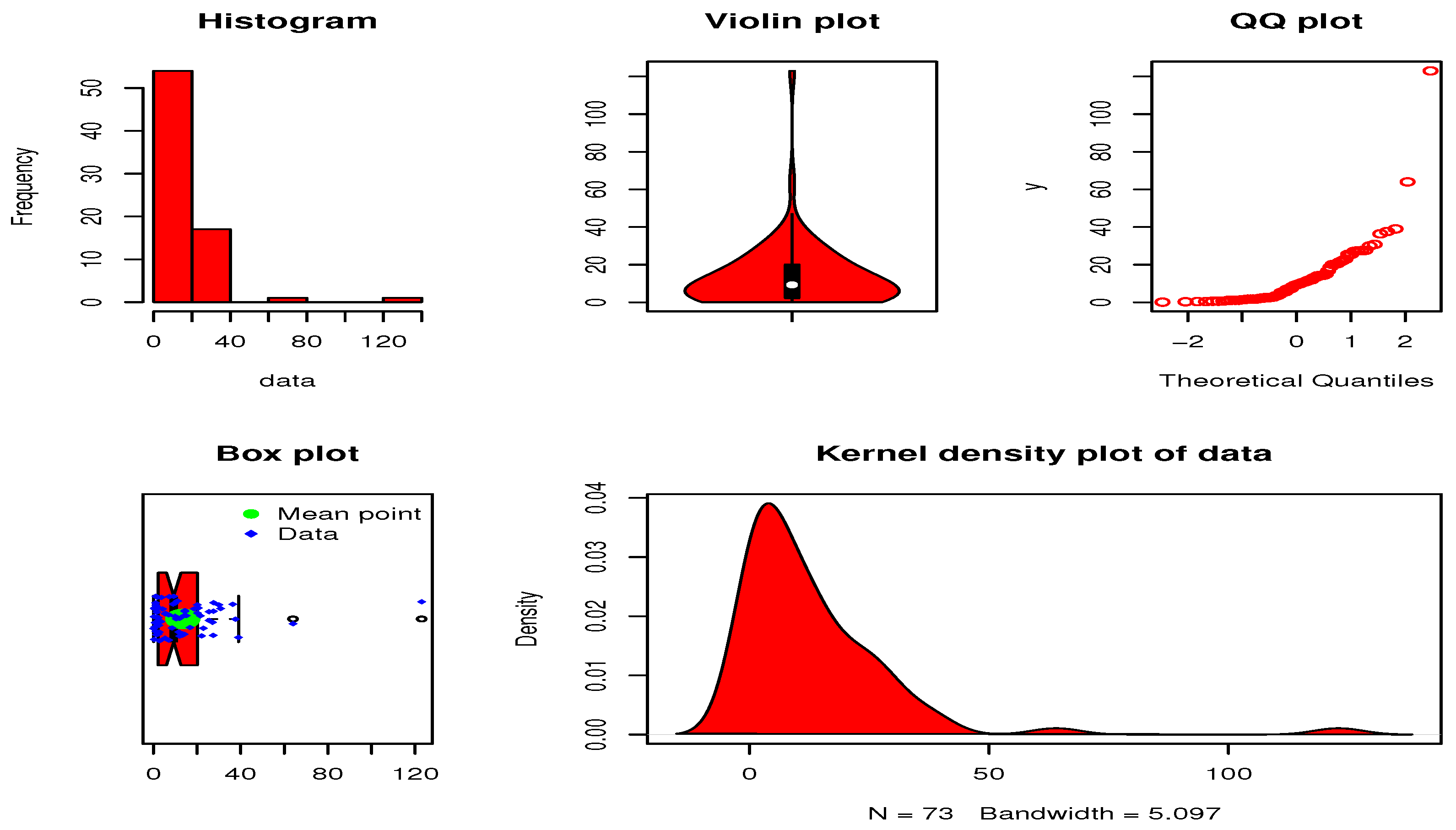
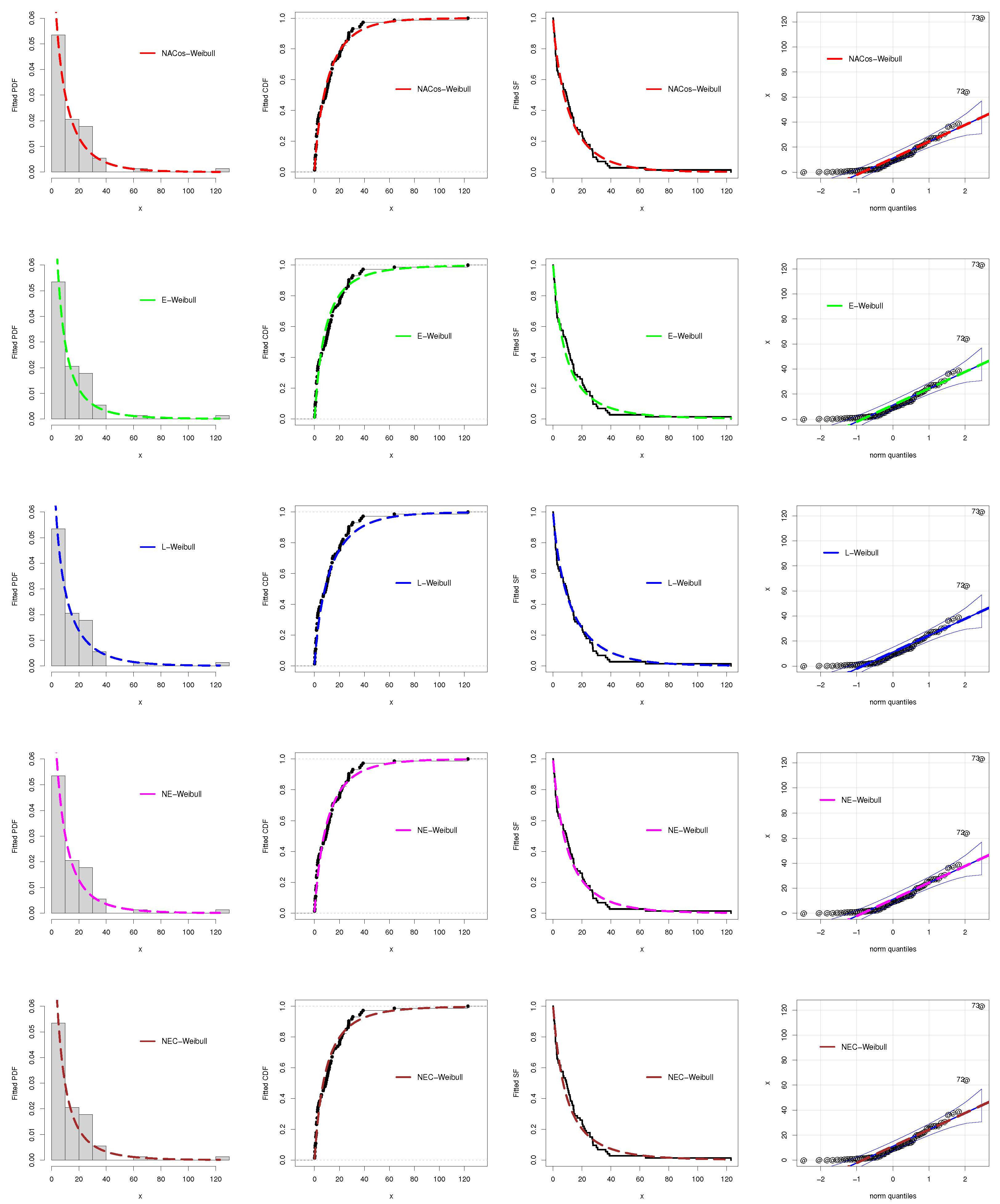
5.1. Analysis of the Hydrological Data Set
5.2. Analysis of the Engineering Data Sets
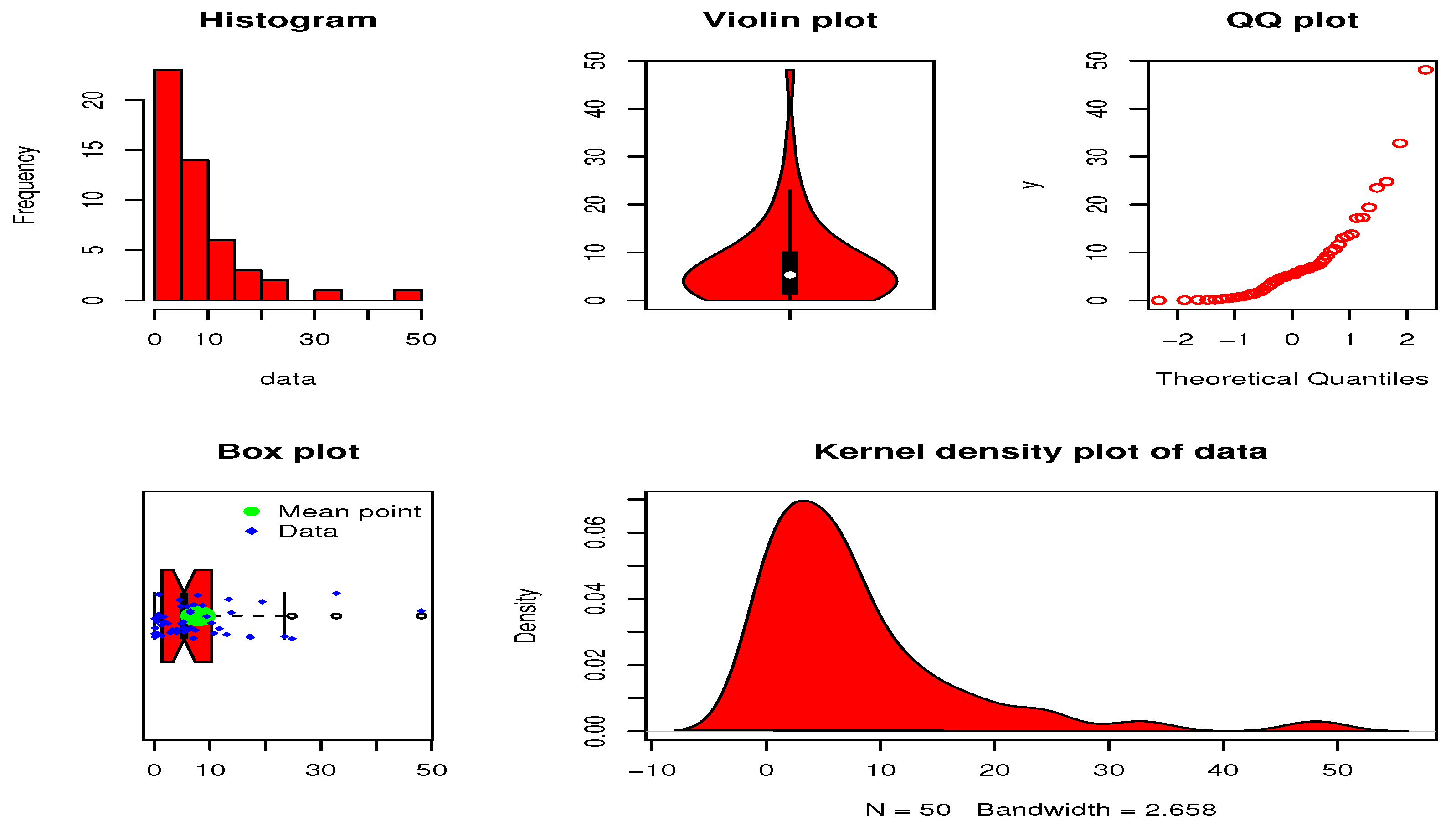
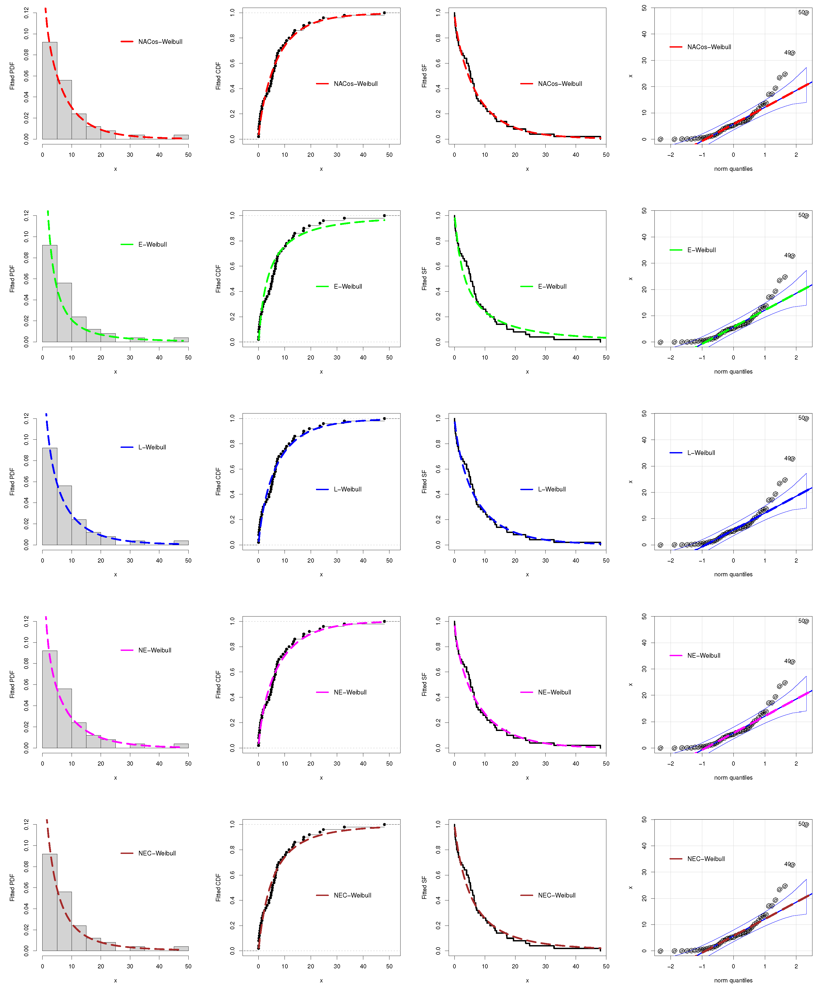
5.2.1. The Failure Times Data
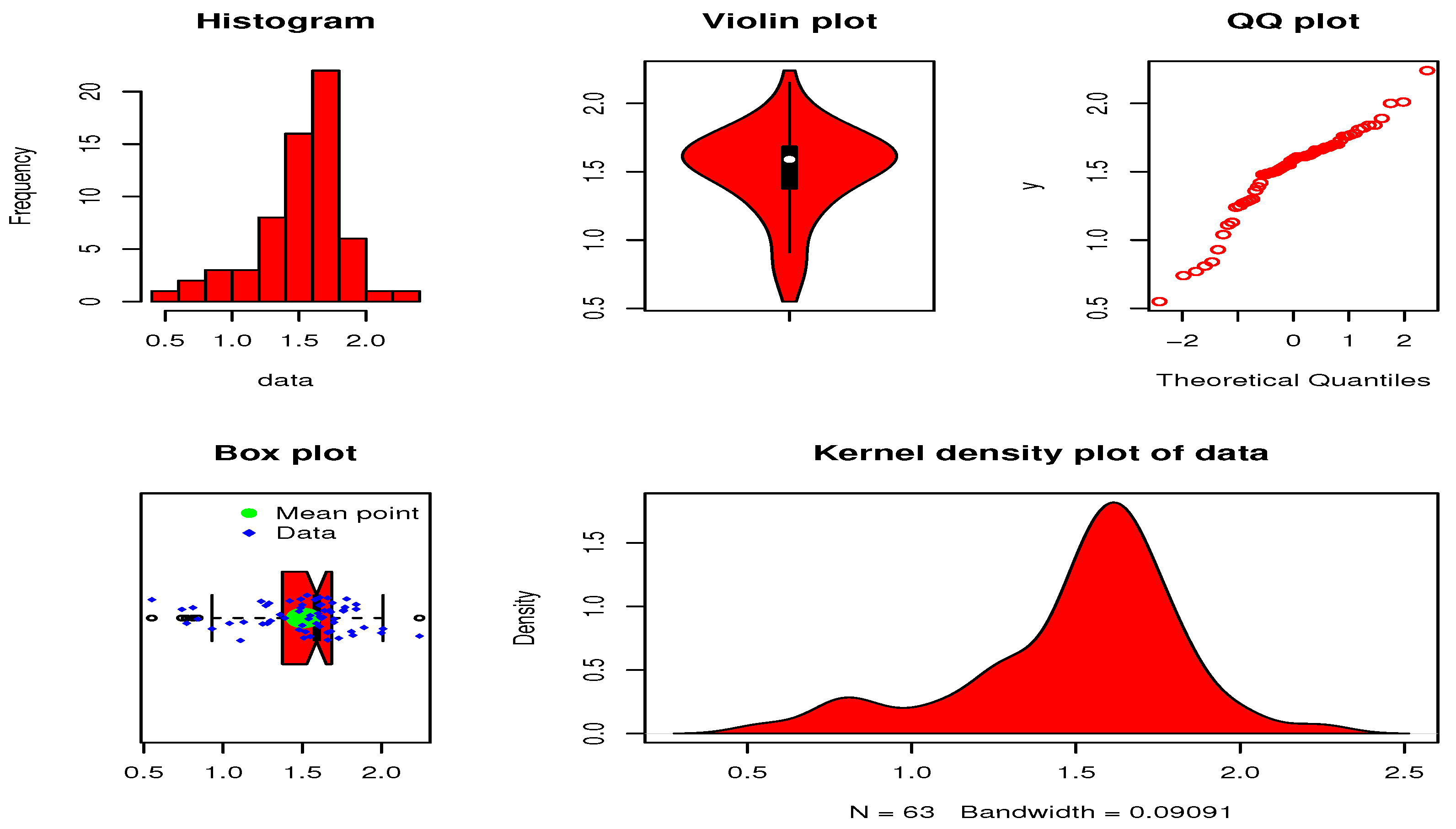
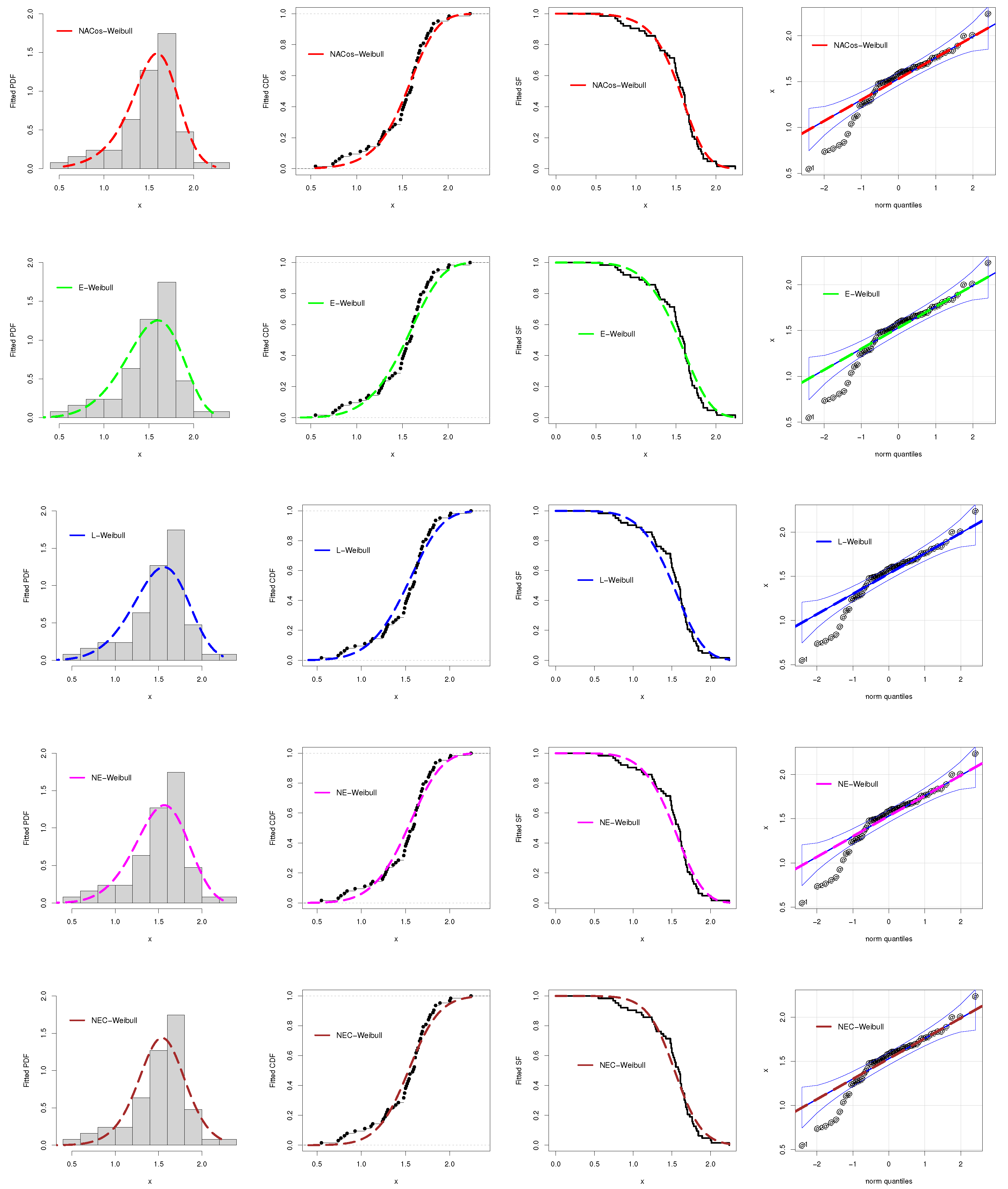
5.2.2. The Glass Fibers Data
6. Conclusions
Author Contributions
Funding
Data Availability Statement
Acknowledgments
Conflicts of Interest
Appendix A. R Code for Simulation Study
References
- Silahli, B.; Dingec, K.D.; Cifter, A.; Aydin, N. Portfolio value-at-risk with two-sided Weibull distribution: Evidence from cryptocurrency markets. Financ. Res. Lett. 2021, 38, 101425. [Google Scholar] [CrossRef]
- Teamah, A.E.A.; Elbanna, A.A.; Gemeay, A.M. Heavy-tailed log-logistic distribution: Properties, risk measures and applications. Stat. Optim. Inf. Comput. 2021, 9, 910–941. [Google Scholar] [CrossRef]
- Ahmad, Z.; Mahmoudi, E.; Dey, S. A new family of heavy tailed distributions with an application to the heavy tailed insurance loss data. Commun. Stat.-Simul. Comput. 2022, 51, 4372–4395. [Google Scholar] [CrossRef]
- Chaito, T.; Khamkong, M. The Length–Biased Weibull–Rayleigh Distribution for Application to Hydrological Data. Lobachevskii J. Math. 2021, 42, 3253–3265. [Google Scholar] [CrossRef]
- Shahmari, M.; Zarafshan, P.; Kouravand, S.; Khashehchi, M. Design and analysis of a combined savonius-darrieus wind turbine for irrigation application. J. Renew. Energy Environ. 2020, 7, 80–86. [Google Scholar]
- Suwarno, S.; Zambak, M.F. The Probability Density Function for Wind Speed Using Modified Weibull Distribution. Int. J. Energy Econ. Policy 2021, 11, 544. [Google Scholar] [CrossRef]
- Al-Babtain, A.A.; Elbatal, I.; Al-Mofleh, H.; Gemeay, A.M.; Afify, A.Z.; Sarg, A.M. The Flexible Burr XG Family: Properties, Inference, and Applications in the Engineering Science. Symmetry 2021, 13, 474. [Google Scholar] [CrossRef]
- Strzelecki, P. Determination of fatigue life for low probability of failure for different stress levels using 3-parameter Weibull distribution. Int. J. Fatigue 2021, 145, 106080. [Google Scholar] [CrossRef]
- Sindhu, T.N.; Atangana, A. Reliability analysis incorporating exponentiated inverse Weibull distribution and inverse power law. Qual. Reliab. Eng. Int. 2021, 37, 2399–2422. [Google Scholar] [CrossRef]
- Abubakar, H.; Muhammad Sabri, S.R. A Simulation Study on Modified Weibull Distribution for Modelling of Investment Return. Pertanika J. Sci. Technol. 2021, 29. [Google Scholar] [CrossRef]
- Kovacs, K.; Ansari, F.; Sihn, W. A modified Weibull model for service life prediction and spare parts forecast in heat treatment industry. Procedia Manuf. 2021, 54, 172–177. [Google Scholar] [CrossRef]
- Liu, X.; Ahmad, Z.; Gemeay, A.M.; Abdulrahman, A.T.; Hafez, E.H.; Khalil, N. Modeling the survival times of the COVID-19 patients with a new statistical model: A case study from China. PLoS ONE 2021, 16, e0254999. [Google Scholar] [CrossRef]
- Dessalegn, Y.; Singh, B.; Vuure, A.W.V.; Badruddin, I.A.; Beri, H.; Hussien, M.; Hossain, N. Investigation of Bamboo Fibrous Tensile Strength Using Modified Weibull Distribution. Materials 2022, 15, 5016. [Google Scholar] [CrossRef] [PubMed]
- Alyami, S.A.; Elbatal, I.; Alotaibi, N.; Almetwally, E.M.; Okasha, H.M.; Elgarhy, M. Topp–Leone Modified Weibull Model: Theory and Applications to Medical and Engineering Data. Appl. Sci. 2022, 12, 10431. [Google Scholar] [CrossRef]
- Bakr, M.E.; Al-Babtain, A.A.; Mahmood, Z.; Aldallal, R.A.; Khosa, S.K.; Abd El-Raouf, M.M.; Hussam, E.; Gemeay, A.M. Statistical modelling for a new family of generalized distributions with real data applications. Math. Biosci. Eng. 2022, 19, 8705–8740. [Google Scholar] [CrossRef] [PubMed]
- Galton, F. Inquiries into Human Faculty and Its Development; Macmillan & Company: London, UK, 1883. [Google Scholar]
- Moors, J.J.A. A quantile alternative for kurtosis. J. R. Stat. Soc. Ser. D 1988, 37, 25–32. [Google Scholar] [CrossRef] [Green Version]
- Bourguignon, M.; Silva, R.B.; Zea, L.M.; Cordeiro, G.M. The Kumaraswamy Pareto distribution. J. Stat. Theory Appl. 2012, 12, 129–144. [Google Scholar] [CrossRef] [Green Version]
- Merovci, F.; Puka, L. Transmuted Pareto distribution. ProbStat Forum 2014, 7, 1–11. [Google Scholar]
- Hameldarbandi, M.; Yilmaz, M. A new perspective of transmuted distribution. Communications Faculty of Sciences University of Ankara Series A1. Math. Stat. 2019, 68, 1144–1162. [Google Scholar]
- Murthy, D.P.; Xie, M.; Jiang, R. Weibull Models; John Wiley & Sons: Hoboken, NJ, USA, 2004. [Google Scholar]
- Smith, R.L.; Naylor, J. A comparison of maximum likelihood and Bayesian estimators for the three-parameter Weibull distribution. J. R. Stat. Soc. Ser. C (Appl. Stat.) 1987, 36, 358–369. [Google Scholar] [CrossRef]


| 0.1, 0.3, 0.4, 0.4, 0.6, 0.6, 0.7, 1.0, 1.1, 1.1, 1.1, 1.4, 1.5, 1.7, 1.7, 1.7, 1.7, 1.9, 2.2, | |||||
| 2.2, 2.5, 2.5, 2.5, 2.7, 2.8, 3.4, 3.6, 4.2, 5.3, 5.3, 5.6, 7.0, 7.0, 7.3, 8.5, 9.0, 9.3, 9.7, | |||||
| 9.9, 10.4, 10.7, 11.0, 11.6, 11.9, 12.0, 13.0, 13.3, 14.1, 14.1, 14.4, 14.4, 15.0, 16.8, | |||||
| 18.7, 20.1, 20.2, 20.6, 21.5, 22.1, 22.9, 25.5, 25.5, 27.1, 27.4, 27.5, 27.6, 30.0, 30.8, | |||||
| 36.4, 37.6, 39.0, 64.0, 123.0. | |||||
| n | Min. | Max. | Median | ||
| 73 | 0.1000 | 123.0000 | 13.4500 | 9.3000 | 315.3845 |
| Skewness | Kurtosis | Range | |||
| 2.2000 | 17.7590 | 20.1000 | 3.6577 | 21.6005 | 122.9000 |
| Models | ||||||
|---|---|---|---|---|---|---|
| NACos-Weibull | 0.8432 | 0.0564 | 0.4754 | - | - | - |
| E-Weibull | 0.5015 | 0.5695 | - | 2.6997 | - | - |
| L-Weibull | 0.7744 | 0.8785 | - | - | 0.1616 | 3.2385 |
| NE-Weibull | 0.9541 | 0.0517 | - | 0.9567 | - | - |
| NEC-Weibull | 0.5823 | 0.3609 | - | - | - | 1.0301 |
| Models | AIC | CVM | AD | KS | p-Value |
|---|---|---|---|---|---|
| NACos-Weibull | 521.8311 | 0.0893 | 0.5456 | 0.0835 | 0.6888 |
| E-Weibull | 526.9967 | 0.1352 | 0.7318 | 0.1056 | 0.3888 |
| L-Weibull | 528.1178 | 0.0941 | 0.5556 | 0.1006 | 0.4500 |
| NE-Weibull | 526.9249 | 0.1066 | 0.6165 | 0.0886 | 0.6147 |
| NEC-Weibull | 526.9782 | 0.1288 | 0.7042 | 0.09599 | 0.5117 |
| 0.013, 0.065, 0.111, 0.111, 0.163, 0.309, 0.426, 0.535, 0.684, 0.747, 0.997, 1.284, 1.304, 1.647, | |||||
| 1.829, 2.336, 2.838, 3.269, 3.977, 3.981, 4.520, 4.789, 4.849, 5.202, 5.291, 5.349, 5.911, 6.018, | |||||
| 6.427, 6.456, 6.572, 7.023, 7.087, 7.291, 7.787, 8.596, 9.388, 10.261, 10.713, 11.658, 13.006, | |||||
| 13.388, 13.842, 17.152, 17.283, 19.418, 23.471, 24.777, 32.795, 48.105 | |||||
| n | Min. | Max. | Median | ||
| 50 | 0.0130 | 48.1050 | 7.8210 | 5.3200 | 84.7559 |
| Skewness | Kurtosis | Range | |||
| 1.3900 | 9.2063 | 10.0430 | 2.3060 | 9.4082 | 48.0920 |
| Models | ||||||
|---|---|---|---|---|---|---|
| NACos-Weibull | 0.6586 | 0.2193 | 3.6914 | - | - | - |
| E-Weibull | 0.3294 | 1.3937 | - | 5.2871 | - | - |
| L-Weibull | 0.7353 | 0.1354 | - | - | 2.1652 | 4.8756 |
| NE-Weibull | 1.5378 | 0.0090 | - | 0.4751 | - | - |
| NEC-Weibull | 0.4197 | 1.0590 | - | - | - | 3.0257 |
| Models | AIC | CVM | AD | KS | p-Value |
|---|---|---|---|---|---|
| NACos-Weibull | 302.5880 | 0.0619 | 0.3121 | 0.0956 | 0.7504 |
| E-Weibull | 315.6884 | 0.2376 | 1.2624 | 0.1762 | 0.0896 |
| L-Weibull | 309.5378 | 0.0864 | 0.4320 | 0.1062 | 0.6251 |
| NE-Weibull | 306.7817 | 0.0725 | 0.3640 | 0.1065 | 0.6216 |
| NEC-Weibull | 310.0237 | 0.1314 | 0.6765 | 0.1177 | 0.4923 |
| 0.55, 0.93, 1.25, 1.36, 1.49, 1.52, 1.58, 1.61, 1.64, 1.68, 1.73, 1.81, 2, 0.74, 1.04, 1.27, | |||||
| 1.53, 1.59, 1.61, 1.66, 1.68, 1.76, 1.82, 2.01, 0.77, 1.11, 1.28, 1.42, 1.5, 1.54, 1.6, 1.62, | |||||
| 1.76, 1.84, 2.24, 0.81, 1.13, 1.29, 1.48, 1.5, 1.55, 1.61, 1.62, 1.66, 1.7, 1.77, 1.84, 0.84, | |||||
| 1.48, 1.51, 1.55, 1.61, 1.63, 1.67, 1.7, 1.78, 1.89 1.39, 1.49, 1.66, 1.69, 1.24, 1.3 | |||||
| n | Min. | Max. | Median | ||
| 63 | 0.5500 | 2.2400 | 1.5070 | 1.5900 | 0.1050 |
| Skewness | Kurtosis | Range | |||
| 1.3750 | 0.3241 | 1.6850 | −0.8999 | 3.92376 | 1.69 |
| Models | ||||||
|---|---|---|---|---|---|---|
| NACos-Weibull | 4.3375 | 0.1124 | 9.3757 | - | - | - |
| E-Weibull | 0.0396 | 0.8297 | - | 6.16298 | - | - |
| L-Weibull | 4.1949 | 0.1132 | - | - | 1.9701 | 1.2117 |
| NE-Weibull | 1.5378 | 0.0090 | - | 0.4751 | - | - |
| NEC-Weibull | 2.7136 | 0.7702 | - | - | - | 5.3487 |
| Models | AIC | CVM | AD | KS | p-Value |
|---|---|---|---|---|---|
| NACos-Weibull | 32.4473 | 0.1585 | 0.8733 | 0.1191 | 0.3331 |
| E-Weibull | 36.1657 | 0.2291 | 1.2613 | 0.1410 | 0.1632 |
| L-Weibull | 38.4442 | 0.2423 | 1.3293 | 0.1700 | 0.0522 |
| NE-Weibull | 36.7869 | 0.2478 | 1.3632 | 0.1557 | 0.0941 |
| NEC-Weibull | 38.7078 | 0.2811 | 1.5398 | 0.1374 | 0.1846 |
Disclaimer/Publisher’s Note: The statements, opinions and data contained in all publications are solely those of the individual author(s) and contributor(s) and not of MDPI and/or the editor(s). MDPI and/or the editor(s) disclaim responsibility for any injury to people or property resulting from any ideas, methods, instructions or products referred to in the content. |
© 2023 by the authors. Licensee MDPI, Basel, Switzerland. This article is an open access article distributed under the terms and conditions of the Creative Commons Attribution (CC BY) license (https://creativecommons.org/licenses/by/4.0/).
Share and Cite
Alghamdi, A.S.; Abd El-Raouf, M.M. A New Alpha Power Cosine-Weibull Model with Applications to Hydrological and Engineering Data. Mathematics 2023, 11, 673. https://doi.org/10.3390/math11030673
Alghamdi AS, Abd El-Raouf MM. A New Alpha Power Cosine-Weibull Model with Applications to Hydrological and Engineering Data. Mathematics. 2023; 11(3):673. https://doi.org/10.3390/math11030673
Chicago/Turabian StyleAlghamdi, Abdulaziz S., and M. M. Abd El-Raouf. 2023. "A New Alpha Power Cosine-Weibull Model with Applications to Hydrological and Engineering Data" Mathematics 11, no. 3: 673. https://doi.org/10.3390/math11030673