Article

Parameter Estimation and Hypothesis Testing of The Bivariate Polynomial Ordinal Logistic Regression Model

1
Department of Statistics, Faculty of Science and Data Analytics, Institut Teknologi Sepuluh Nopember, Surabaya 60111, Indonesia
2
Department of Mathematics, Faculty of Science and Technology, Universitas Airlangga, Surabaya 60115, Indonesia
*
Author to whom correspondence should be addressed.
Mathematics 2023, 11(3), 579; https://doi.org/10.3390/math11030579
Submission received: 22 November 2022 / Revised: 7 January 2023 / Accepted: 18 January 2023 / Published: 21 January 2023
(This article belongs to the Special Issue Advances in Applied Probability and Statistical Inference)

Abstract

:
Logistic regression is one of statistical methods that used to analyze the correlation between categorical response variables and predictor variables which are categorical or continuous. Many studies on logistic regression have been carried out by assuming that the predictor variable and its logit link function have a linear relationship. However, in several cases it was found that the relationship was not always linear, but could be quadratic, cubic, or in the form of other curves, so that the assumption of linearity was incorrect. Therefore, this study will develop a bivariate polynomial ordinal logistic regression (BPOLR) model which is an extension of ordinal logistic regression, with two correlated response variables in which the relationship between the continuous predictor variable and its logit is modeled as a polynomial form. There are commonly two correlated response variables in scientific research. In this study, each response variable used consisted of three categories. This study aims to obtain parameter estimators of the BPOLR model using the maximum likelihood estimation (MLE) method, obtain test statistics of parameters using the maximum likelihood ratio test (MLRT) method, and obtain algorithms of estimating and hypothesis testing for parameters of the BPOLR model. The results of the first partial derivatives are not closed-form, thus, a numerical optimization such as the Berndt–Hall–Hall–Hausman (BHHH) method is needed to obtain the maximum likelihood estimator. The distribution statistically test is followed the Chi-square limit distribution, asymptotically.

1. Introduction

The logistic regression model is one of statistical methods which is used to analyze the correlation between categorical response variables and predictor variables that are categorical or continuous. If the response variable has more than two categories and there are levels in that category (ordinal scale), then an ordinal logistic regression model is used [1]. The logistic regression modeling often does not involve only one response variable because of a phenomenon involving multiple response variables. Logistic regression involving one response variable is called univariate logistic regression. Meanwhile, logistic regression that involves two or more response variables and correlates between response variables is called multivariate logistic regression. Especially for multivariate logistic regression involving two correlated response variables, it is called the bivariate logistic regression.
Several studies on ordinal logistic regression have been carried out for bivariate cases. Dale [2] has studied parameter estimationusing the MLE method. Williamson et al. [3] used the generalized estimating equation (GEE) method, whereas Enea and Lovison [4] used penalized MLE for the parameter estimation of bivariate ordinal logistic regression models. The previous studies examined logistic regression modeling by assuming that the continuous predictor variable and its logit link function have a linear relationship. However, the reality is that in some cases it is found that the relationship is not always linear, but can be quadratic, cubic, or other curves, so that the assumption of linearity is incorrect.
Royston and Altman [5] introduced the fractional polynomial approach, which is one of the development of a polynomial model, to understand the functional form of a continuous predictor variable. This model involves a more flexible relationship that can be linear or non-linear and has been used by several researchers [6,7,8,9]. In its development, several studies have examined the use of fractional polynomials in logistic regression analysis [10,11,12]. However, these previous studies were limited to univariate binary logistic regression. Furthermore, the bivariate binary logistic regression has been developed but limited to the second order [13]. Therefore, we propose an extension of ordinal logistic regression with two correlated response variables in which the relationship between the continuous predictor variable and its logit is modeled as a polynomial form. The proposed model is called the bivariate polynomial ordinal logistic regression (BPOLR) model. This study aimed to obtain parameter estimators of the BPOLR model using the MLE method, obtain test statistics of parameters using the MLRT method, and obtain algorithms of estimating and hypothesis testing for parameters of the BPOLR model.
An example of applying the BPOLR model can be applied to modeling the nutritional status of toddlers. Based on Narendra et al. [14], children from birth to about one year old have growth that increases rapidly and then decreases slowly as the child gets older. Therefore, the polynomial approach is more suitable for modeling child growth [15]. Tilling et al. [16] modeled child growth using the fractional polynomial approach and concluded that the model with the fractional polynomial approach shows a growth rate that is initially fast and then slows down over time.
The following discussion in this paper is divided into several main topics. In Section 2, we introduce the BPOLR model followed by parameter estimation using the MLE method in Section 3. We present simultaneous hypothesis testing in Section 4 to test the significance of all parameters together using the MLRT method and we present a simulation study in Section 5. Furthermore, Section 6 contains conclusions.

2. The Bivariate Polynomial Ordinal Logistic Regression (BPOLR) Model

The BPOLR model is an expansion of the ordinal logistic regression model when there are two correlated ordinal response variables and the relationship between the continuous predictor variable and its logit is modeled as a polynomial form. In this study, the response variables used each have 3 categories. Let Y1 and Y2 be response variables which have a value of 1; 2; or 3, then Y ab = Y 1 = a , Y 2 = b   ;   a , b = 1 , 2 , 3 are random variables that have their respective probabilities π ab   , as presented in Table 1 below.
Based on Table 1, the random vector y = Y 11 Y 12 Y 13 Y 21 Y 22 Y 23 Y 31 Y 32 have a multinomial distribution so it has a joint probability density function as follows:
P Y 11 = y 11 , Y 12 = y 12 , , Y 32 = y 32 = a = 1 3 b = 1 3 π ab y ab
where 0 < π ab < 1 ; a , b = 1 , 2 , 3 ; y ab = 0 , 1 ; a = 1 3 b = 1 3 Y ab = 1 ; and a = 1 3 b = 1 3 π ab = 1 . π ab = P Y 1 = a , Y 2 = b is the joint probability of the response variables. π a = b = 1 3 P Y 1 = a , Y 2 = b is the marginal probability for the variable Y 1 and π b = a = 1 3 P Y 1 = a , Y 2 = b is the marginal probability for the variable Y 2 .
The model that can be used for ordinal logistic regression is the cumulative logit model. In this study, the BPOLR model has two ordinal-scale response variables that are correlated with each other and each has 3 categories, so we have the cumulative probability for Y 1 and Y 2 , i.e., P Y 1 a x ; a = 1 , 2 and P Y 2 b x ; b = 1 , 2 . Let F a x = P Y 1 a x ; a = 1 , 2 is the marginal cumulative probability of variable Y 1 given x , F b x = P Y 2 b x ; b = 1 , 2 is the marginal cumulative probability of variable Y 2 given x and F ab x = P Y 1 a , Y 2 b x ; a , b = 1 , 2 is the joint cumulative probability between variables Y 1 and Y 2 given x , so we have the BPOLR model as follows:
  • The cumulative logit model for Y 1
    g 1 = logit P Y 1 1 x = logit F 1 x = ln F 1 x 1 F 1 x = α 11 + j = 1 k β 1 j T x j r j *  
    g 2 = logit P Y 1 2 x = logit F 2 x = ln F 2 x 1 F 2 x = α 12 + j = 1 k β 1 j T x j r j *
  • The cumulative logit model for Y 2
    g 3 = logit P Y 2 1 x = logit F 1 x = ln F 1 x 1 F 1 x = α 21 + j = 1 k β 2 j T x j r j *
    g 4 = logit P Y 2 2 x = logit F 2 x = ln F 2 x 1 F 2 x = α 22 + j = 1 k β 2 j T x j r j *
  • The odds ratio transformation model for Y 1 and Y 2
    g 5 = ln ψ 11 x = ln F 11 x 1 F 1 x F 1 x + F 11 x F 1 x F 11 x F 1 x F 11 x = Δ 11 + j = 1 k γ j T x j r j *
    g 6 = ln ψ 12 x = ln F 12 x 1 F 1 x F 2 x + F 12 x F 1 x F 12 x F 2 x F 12 x = Δ 12 + j = 1 k γ j T x j r j *
    g 7 = ln ψ 21 x = ln F 21 x 1 F 2 x F 1 x + F 21 x F 2 x F 21 x F 1 x F 21 x = Δ 21 + j = 1 k γ j T x j r j *
    g 8 = ln ψ 22 x = ln F 22 x 1 F 2 x F 2 x + F 22 x F 2 x F 22 x F 2 x F 22 x = Δ 22 + j = 1 k γ j T x j r j *
    where α 1 a , α 2 b , Δ ab   ;   a , b = 1 , 2 are the intercept parameters with α 11 < α 12 and α 21 < α 22 ; β 1 j , β 2 j and γ j are vector of parameters for the j-th predictor variable, which are symbolized by β 1 j = β 01 j β 11 j β r 1 j T , β 2 j = β 02 j β 12 j β r 2 j T , γ j = γ 0 j γ 1 j γ r j T . x is vector of predictor variable with x = 1 x 1 r 1 * x k r k * T where x j r j * = 1 x j x j 2 x j r j T is vector of the j-th predictor variable with the r-th degree of polynomial.
Based on Equations (2)–(5), the marginal cumulative probability of variable Y 1 and Y 2 can be obtained from the following equation:
P Y 1 a x = F a · x = exp α 1 a + j = 1 k β 1 j T x j r j * 1 + exp α 1 a + j = 1 k β 1 j T x j r j * ;   a = 1 , 2
P Y 2 b x = F · b x = exp α 2 b + j = 1 k β 2 j T x j r j * 1 + exp α 2 b + j = 1 k β 2 j T x j r j *   ;   b = 1 , 2
ψ ab x is the odds ratio (OR), a measure of association that can indicate a correlation between the response variables. The OR value is formulated as follows:
ψ ab x = P Y 1 a , Y 2 b x P Y 1 > a , Y 2 > b x P Y 1 > a , Y 2 b x P Y 1 a , Y 2 > b x = F ab x 1 F a x F b x + F ab x F a x F ab x F b x F ab x
where F ab x can be obtained from:
F ab x = c c 2 + d 2 ψ ab x 1 ,   ψ ab x 1 F a x F b x ,   ψ ab x = 1
where a , b = 1 , 2 ; c = 1 + ψ ab x 1 F a x + F b x and d = 4 ψ ab x ψ ab x 1 F a x F b x .
Next, the joint probability of the response variables, π ab , can be obtained as follows:
π 11 = F 11 ; π 12 = F 12 F 11 ; π 13 = F 1 F 12 ; π 21 = F 21 F 11 ; π 22 = F 22 F 12 F 21 + F 11 ; π 23 = F 2 F 22 F 1 + F 12 ; π 31 = F 1 F 21 ; π 32 = F 2 F 22 F 1 + F 21 ; π 33 = 1 F 2 F 2 + F 22 .

3. Parameter Estimation of The BPOLR Model

In this study, the parameter estimation of the BPOLR model was carried out using the maximum likelihood estimation (MLE) method. The principle of the MLE method is to estimate the parameters of the BPOLR model, namely:
θ = α 11 α 12 β 011 β 111 β r 1 k α 21 α 22 β 021 β 121 β r 2 k Δ 11 Δ 12 Δ 21 Δ 22 γ 01 γ 11 γ r k T
obtained by maximizing the likelihood function. Based on Equation (1), the likelihood function is obtained as follows:
L θ = i = 1 n a = 1 3 b = 1 3 π abi y abi
To simplify the calculation, an ln transformation is carried out on the likelihood function so that the ln-likelihood function is formed as follows:
Q = lnL θ = i = 1 n a = 1 3 b = 1 3 y abi ln π abi = i = 1 n y 11 i ln π 11 i + y 12 i ln π 12 i + + y 33 i ln π 33 i
the next step of the ln-likelihood function is the first partial derivative of the parameter to be estimated and then equated with zero. The results of the first partial derivative of the ln-likelihood function with respect to its parameters are as follows:
  • The first partial derivative of the ln-likelihood function to the parameter α 11
    α 11 = i = 1 n y 11 i π 11 i y 12 i π 12 i y 21 i π 21 i + y 22 i π 22 i δ 11 i + y 12 i π 12 i y 13 i π 13 i y 22 i π 22 i + y 23 i π 23 i δ 12 i + y 13 i π 13 i y 23 i π 23 i ξ 1 i
  • The first partial derivative of the ln-likelihood function to the parameter α 12
    α 12 = i = 1 n y 21 i π 21 i y 22 i π 22 i y 31 i π 31 i + y 32 i π 32 i δ 21 i + y 22 i π 22 i y 23 i π 23 i y 32 i π 32 i + y 33 i π 33 i δ 22 i + y 23 i π 23 i y 33 i π 33 i ξ 2 i
  • The first partial derivative of the ln-likelihood function to the parameter β 1 j ;   j = 1 , 2 , , k
    β 1 j = i = 1 n y 11 i π 11 i y 12 i π 12 i y 21 i π 21 i + y 22 i π 22 i δ 11 i + y 12 i π 12 i y 13 i π 13 i y 22 i π 22 i + y 23 i π 23 i δ 12 i + y 13 i π 13 i y 23 i π 23 i ξ 1 i x j r j * + y 21 i π 21 i y 22 i π 22 i y 31 i π 31 i + y 32 i π 32 i δ 21 i + y 22 i π 22 i y 23 i π 23 i y 32 i π 32 i + y 33 i π 33 i δ 22 i + y 23 i π 23 i y 33 i π 33 i ξ 2 i x j r j *
  • The first partial derivative of the ln-likelihood function to the parameter α 21
    α 21 = i = 1 n y 11 i π 11 i y 12 i π 12 i y 21 i π 21 i + y 22 i π 22 i μ 11 i + y 21 i π 21 i y 22 i π 22 i y 31 i π 31 i + y 32 i π 32 i μ 21 i + y 31 i π 31 i y 32 i π 32 i ξ 1 i
  • The first partial derivative of the ln-likelihood function to the parameter α 22
    α 22 = i = 1 n y 12 i π 12 i y 13 i π 13 i y 22 i π 22 i + y 23 i π 23 i μ 12 i + y 22 i π 22 i y 23 i π 23 i y 32 i π 32 i + y 33 i π 33 i μ 22 i + y 32 i π 32 i y 33 i π 33 i ξ 2 i
  • The first partial derivative of the ln-likelihood function to the parameter β 2 j ;   j = 1 , 2 , , k
    β 2 j = i = 1 n y 11 i π 11 i y 12 i π 12 i y 21 i π 21 i + y 22 i π 22 i μ 11 i + y 21 i π 21 i y 22 i π 22 i y 31 i π 31 i + y 32 i π 32 i μ 21 i + y 31 i π 31 i y 32 i π 32 i ξ 1 i x j r j * + y 12 i π 12 i y 13 i π 13 i y 22 i π 22 i + y 23 i π 23 i μ 12 i + y 22 i π 22 i y 23 i π 23 i y 32 i π 32 i + y 33 i π 33 i μ 22 i + y 32 i π 32 i y 33 i π 33 i ξ 2 i x j r j *
  • The first partial derivative of the ln-likelihood function to the parameter Δ 11
    Δ 11 = i = 1 n y 11 i π 11 i y 12 i π 12 i y 21 i π 21 i + y 22 i π 22 i z 11 i ψ 11 i
  • The first partial derivative of the ln-likelihood function to the parameter Δ 12
    Δ 12 = i = 1 n y 12 i π 12 i y 13 i π 13 i y 22 i π 22 i + y 23 i π 23 i z 12 i ψ 12 i
  • The first partial derivative of the ln-likelihood function to the parameter Δ 21
    Δ 21 = i = 1 n y 21 i π 21 i y 22 i π 22 i y 31 i π 31 i + y 32 i π 32 i z 21 i ψ 21 i
  • The first partial derivative of the ln-likelihood function to the parameter Δ 22
    Δ 22 = i = 1 n y 22 i π 22 i y 23 i π 23 i y 32 i π 32 i + y 33 i π 33 i z 22 i ψ 22 i
  • The first partial derivative of the ln-likelihood function to the parameter γ j ;   j = 1 , 2 , , k
    γ j = i = 1 n y 11 i π 11 i y 12 i π 12 i y 21 i π 21 i + y 22 i π 22 i z 11 i ψ 11 i + y 12 i π 12 i y 13 i π 13 i y 22 i π 22 i + y 23 i π 23 i z 12 i ψ 12 i + y 21 i π 21 i y 22 i π 22 i y 31 i π 31 i + y 32 i π 32 i z 21 i ψ 21 i + y 22 i π 22 i y 23 i π 23 i y 32 i π 32 i + y 33 i π 33 i z 22 i ψ 22 i x j r j *
    where δ ab = 1 2 1 S ab 1 1 + ψ ab F a F b F a F b ; μ ab = 1 2 1 S ab 1 1 + ψ ab F b F a F a F b
S ab = 1 + ψ ab 1 F a + F b 2 4 ψ ab ψ ab 1 F a F b 1 2 ; ξ a = F a 1 F a ; ξ b = F b 1 F b
z ab = 2 ψ ab 1 2 S ab 1 1 S ab + ψ ab 1 F a + F b 2 F a F b .
The result of the first partial derivatives are not closed-form, thus, a numerical optimization such as the Berndt–Hall–Hall–Hausman (BHHH) method is needed to obtain the maximum likelihood estimators and the BHHH algorithm is as follows:
  • Step 1. Determine the initial value for
    θ ( 0 ) = α 11 ( 0 ) α 12 ( 0 ) β 011 ( 0 ) β 111 ( 0 ) β r 1 k ( 0 ) α 21 ( 0 ) α 22 ( 0 ) β 021 ( 0 ) β 121 ( 0 ) β r 2 k ( 0 )
    Δ 11 ( 0 ) Δ 12 ( 0 ) Δ 21 ( 0 ) Δ 22 ( 0 ) γ 01 ( 0 ) γ 11 ( 0 ) γ r k ( 0 ) T
    obtained from the parameter estimator of the ordinal logistic regression model on each response variable.
  • Step 2. Calculate the gradient vector elements obtained from the first partial derivative of the ln-likelihood function for each parameter
    q θ = α 11 α 12 β 011 β 111 β r 1 k α 21 α 22 β 021 β 121 β r 2 k
    Δ 11 Δ 12 Δ 21 Δ 22 γ 01 γ 11 γ r k T
  • Step 3. Calculate the Hessian matrix H θ that can be obtained from the following formula
    H θ = q T θ q θ
  • Step 4. Start the BHHH iteration process with the following formula
    θ ^ ( t + 1 ) = θ ^ ( t ) H 1 θ ^ ( t ) q θ ^ ( t ) ,   for   t = 0 , 1 , 2 , . . . .
  • Step 5. The iteration will stop if θ ^ ( t + 1 ) θ ^ ( t ) < ε , where ε is a very small positive number. The last iteration produces an estimator value for each parameter.
Furthermore, the best model in this study is determined using the criteria of Akaike information criterion corrected (AICc), Bayesian information criterion (BIC), and deviance which are defined as follows:
A I C c = 2 ln L θ ^ + 2 K + 2 K K + 1 n K 1
B I C = 2 ln L θ ^ + K ln n
D e v i a n c e = 2 ln L θ ^
where L θ ^ is the likelihood value of the parameter’s estimate, K is the number of covariates, and 𝑛 is the sample size. The best model is the BPOLR model, which has the smallest values of AICc, BIC, and deviance.

4. Hypothesis Testing of The BPOLR Model

The simultaneous hypothesis testing of the BPOLR model aims to determine the influence of the predictor variable on the response variable simultaneously or to discover at least one predictor variable which has a significant effect against the response variable. The hypothesis used is as follows:
H 0 : β p 1 q = β p 2 q = γ p q = 0   ;   p = 1 , 2 , , r q   ;   q = 1 , 2 , , k  
H 1 :   at   least   one   β p 1 q 0   or   β p 2 q 0   or   γ p q 0
In this study, we used the MLRT method to obtain the test statistics by calculating the ratio between the maximum value of the likelihood function under H 0 , L ω , with the maximum value of the likelihood function under population, L Ω .
The first step to obtaining the maximum value of L ω is to define the parameter space under H 0 , ω = α 11 , α 12 , α 21 , α 22 , Δ 11 , Δ 12 , Δ 21 , Δ 22 , β 011 , , β 01 k , β 021 , , β 02 k , γ 01 , , γ 0 k . The likelihood function under H 0 is:
L ω = i = 1 n a = 1 3 b = 1 3 π a b i * y a b i
Let ω = ln L ω , then the log-likelihood function under H 0 is
ω = i = 1 n y 11 i ln π 11 i * + y 12 i ln π 12 i * + + y 33 i ln π 33 i *
Furthermore, we can obtain the estimated value of the maximum log-likelihood function under H 0 :
ω ^ = i = 1 n y 11 i ln π ^ 11 i * + y 12 i ln π ^ 12 i * + + y 33 i ln π ^ 33 i *
where
π ^ 11 i * = F ^ 11 i *   ;   π ^ 12 i * = F ^ 12 i * F ^ 11 i * ;   π ^ 13 i * = F ^ 1 i * F ^ 12 i * ;   π ^ 21 i * = F ^ 21 i * F ^ 11 i * ;
π ^ 22 i * = F ^ 22 i * F ^ 12 i * F ^ 21 i * + F ^ 11 i *   ; π ^ 23 i * = F ^ 2 i * F ^ 1 i * F ^ 22 i * + F ^ 12 i * ; π ^ 31 i * = F ^ 1 i * F ^ 21 i * ;
π ^ 32 i * = F ^ 2 i * F ^ 22 i * F ^ 1 i * + F ^ 21 i * ;   π ^ 33 i * = 1 F ^ 2 i * F ^ 2 i * + F ^ 22 i *
with
F ^ abi * = p 3 p 3 2 + q 3 2 ψ ^ ab 1 , ψ ^ ab 1 ;   p 3 = 1 + ψ ^ ab 1 F ^ a i * + F ^ bi * ;   q 3 = 4 ψ ^ ab ψ ^ ab 1 F ^ a i * F ^ bi *
F ^ a i * = exp α ^ 1 a + j = 1 k β ^ 01 j exp α ^ 1 a + j = 1 k β ^ 01 j ; F ^ bi * = exp α ^ 2 b + j = 1 k β ^ 02 j exp α ^ 2 b + j = 1 k β ^ 02 j ; ψ ^ 11 = n 11 i n 22 i + n 23 i + n 32 i + n 33 i n 12 i + n 13 i n 21 i + n 31 i   ;
ψ ^ 12 = n 11 i + n 12 i n 23 i + n 33 i n 13 i n 21 i + n 22 i + n 31 i + n 32 i ; ψ ^ 21 = n 11 i + n 21 i n 32 i + n 33 i n 12 i + n 13 i + n 22 i + n 23 i n 31 i ; ψ ^ 22 = n 11 i + n 12 i + n 21 i + n 22 i n 33 i n 13 i + n 23 i n 31 i + n 32 i .
Furthermore, to obtain the maximum value of L Ω is to define the parameter space under population, Ω = α 11 , α 12 , α 21 , α 22 , Δ 11 , Δ 12 , Δ 21 , Δ 22 , β p 1 q , β p 2 q , γ p q ; p = 0 , 1 , 2 , , r q ; q = 1 , 2 , , k . Then, the likelihood function under population is
L Ω = i = 1 n a = 1 3 b = 1 3 π a b i y a b i
Let Ω = ln L Ω , then the log-likelihood function under population is
Ω = i = 1 n y 11 i ln π 11 i + y 12 i ln π 12 i + + y 33 i ln π 33 i
Furthermore, we can obtain the estimated value of the maximum log-likelihood function under population, that is:
Ω ^ = i = 1 n y 11 i ln π ^ 11 i + y 12 i ln π ^ 12 i + + y 33 i ln π ^ 33 i
The test statistic using MLRT method is obtained by
G 2 = 2 ln L ω ^ L Ω ^ = 2 Ω ^ ω ^
where ω ^ and Ω ^ are given in Equations (36) and (39), respectively. Furthermore, the test statistic in Equation (38) can be expressed as follows
G 2 = 2 i = 1 n y 11 i ln π ^ 11 i π ^ 11 i * + y 12 i ln π ^ 12 i π ^ 12 i * + + y 33 i ln π ^ 33 i π ^ 33 i * = 2 i = 1 n n π ^ 11 i ln 1 + π ^ 11 i π ^ 11 i * π ^ 11 i * + i = 1 n n π ^ 12 i ln 1 + π ^ 12 i π ^ 12 i * π ^ 12 i * + + i = 1 n n π ^ 33 i ln 1 + π ^ 33 i π ^ 33 i * π ^ 33 i *
Based on the Taylor expansion of ln 1 + π ^ a b i π ^ a b i * π ^ a b i * with a , b = 1 , 2 , 3 and i = 1 , 2 , , n it will be proved that lim n G 2 = G * .
G * = i = 1 n n π ^ 11 i n π ^ 11 i * 2 n π ^ 11 i * + i = 1 n n π ^ 12 i n π ^ 12 i * 2 n π ^ 12 i * + + i = 1 n n π ^ 33 i n π ^ 33 i * 2 n π ^ 33 i * = i = 1 n a = 1 3 b = 1 3 n π ^ a b i n π ^ a b i * 2 n π ^ a b i * = i = 1 n a = 1 3 b = 1 3 y a b i n π ^ a b i * 2 n π ^ a b i *
The test statistic in Equation (39) has an asymptotic Chi-square limit distribution with v degree of freedom, where v is the difference between the number of parameters in the BPOLR model under population and H 0 , v = 8 + 3 j = 1 k r j + k 8 + 3 k = 3 j = 1 k r j . Therefore, reject H 0 when G 2 > χ v , 1 α 2 , where χ v , 1 α 2 is the 1 α quantile from a Chi-square distribution ( χ 2 ) with 𝑣 degree of freedom.

5. Simulation Study

In this section, we outline a simulation study for the present performance of parameter estimation of the BPOLR model based on the BHHH algorithm. The simulation was constructed by two ordinal response variables that each have three categories and three predictor variables. In this paper, the simulation is carried out for one example of the BPOLR model, i.e., the BPOLR model with degree polynomial (1,2,1). The simulation was carried out for 100 replications with different sample sizes, i.e., n = 100, n = 200, and n = 300. The simulation scenarios are decided as follows:
  • Generate three predictor variables (X1, X2 and X3) that are constructed from a standard uniform distribution
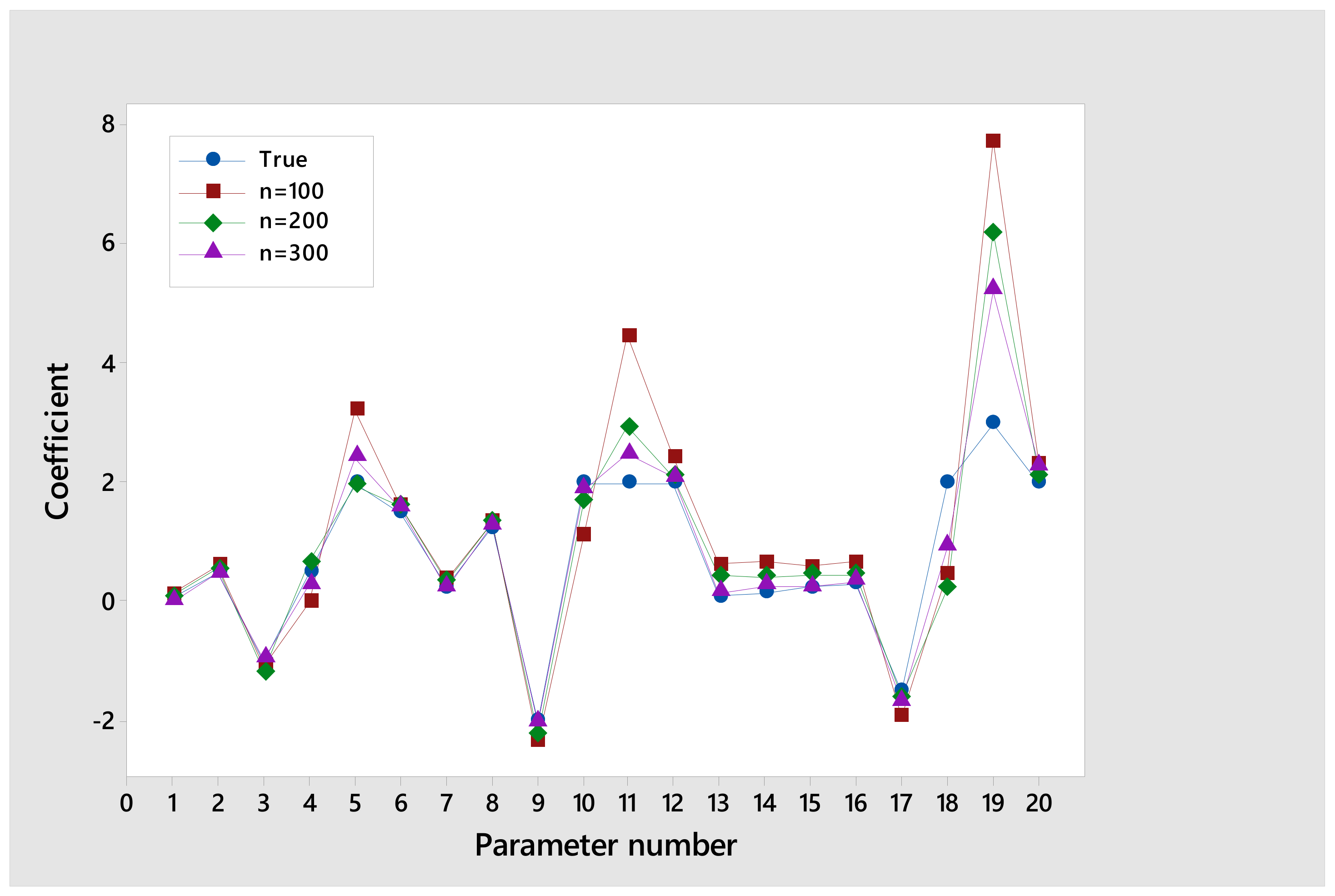
  • Set the initial coefficients of the BPOLR model as follows:
    α 11 = 0.05   ;   α 12 = 0.5   ;   β 111 = 1   ;   β 112 = 0.5   ;   β 212 = 2   ;   β 113 = 1.5   ;   α 21 = 0.25   ;   α 22 = 1.25   ;
    β 121 = 2   ;   β 122 = 2   ;   β 222 = 2   ;   β 123 = 2   ;   Δ 11 = 0.1   ;   Δ 12 = 0.15   ;   Δ 21 = 0.25   ;   Δ 22 = 0.3   ;  
    γ 11 = 1.5   ;   γ 12 = 2   ;   γ 22 = 3   ;   γ 13 = 2
  • Generate two ordinal response variables (Y1 and Y2) with the following steps:
    Determine the cumulative logit model for Y1 and Y2 as in Equations (2)–(5) and the odds ratio transformation model, as in Equations (6)–(9)
    Determine the marginal cumulative probability for Y1 and Y2 as in Equations (10) and (11) and the joint cumulative probability as in Equation (13).
    Determine the joint probability of Y1 and Y2
    Generate two ordinal response variables based on the joint probabilty obtained
  • Examine the independence of the response variables using the Mantel–Haenszel test to fulfill the assumption of dependence between the response variables in the bivariate model. If the response variable is independent, then the data generation process is repeated until the dependent response variable is obtained.
  • Estimate the parameters of the BPOLR model based on the BHHH algorithm
  • Repeat the process for up to 100 replications for each sample size
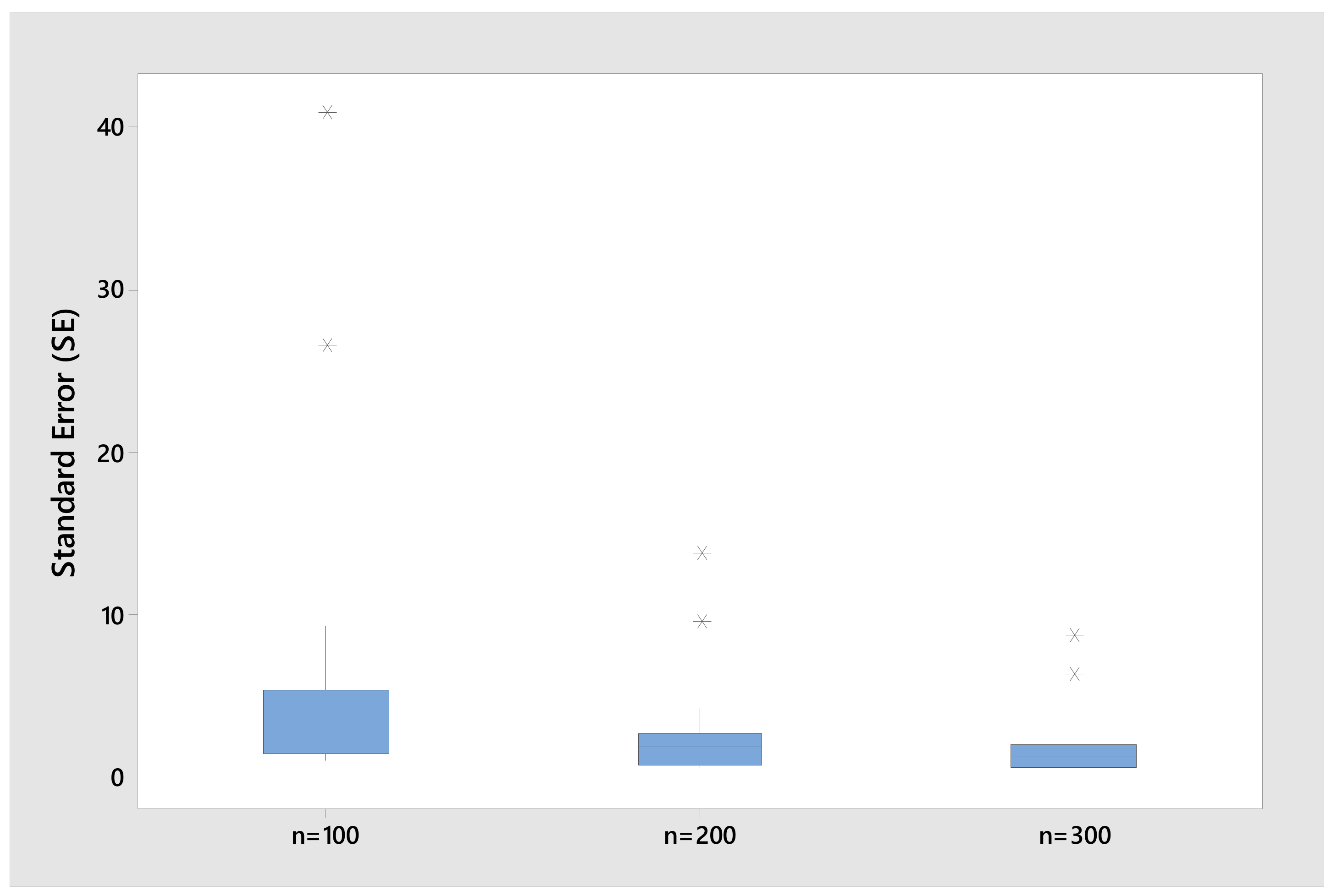
  • Calculate the mean of parameter estimated and its standard error (SE)
The results and comments regarding the simulation study are given in the following tables and figures below. The mean of the estimated parameters and their corresponding standard error (SE) for different sample sizes are presented in Table 2. The results show that the estimated parameters approach their true coefficient on average and the corresponding standard errors also decrease as the sample size increases.
Furthermore, the suitability of the estimated parameter with the true coefficients for each sample size can be presented in Figure 1 below:
Based on Figure 1, the results show that the greater of samples size, the closer the estimated parameter values get to the true coefficient values. This can be seen from the movement of the estimated parameter coefficients for n = 300, which are closest to the true coefficients, and for n = 100, the coefficients which are farthest for each parameter. In addition, the standard error range values from parameter estimation was also investigated for different samples in the form of boxplots. When the sample size increases, the standard error values of the model parameter estimation becomes less, as presented in Figure 2 as follows:

6. Conclusions

We developed ordinal logistic regression with two correlated response variables in which the relationship between the continuous predictor variable and its logit is modeled as a polynomial form, called the BPOLR model. The proposed BPOLR model contributes to the development of statistical science that can be used as an alternative solution in statistical modeling related to the bivariate ordinal logistic regression, where the relationship between continuous predictor variables and their logit links is assumed to be not always linear, so that it is more flexible. Therefore, the advantage of the BPOLR model can accommodate linear, quadratic, cubic or other relationships between continuous predictor variables and their logit links in a model. We used the MLE method to obtain parameter estimators of the BPOLR model. The first partial derivatives are not closed-form, thus, a numerical optimization such as the method of BHHH is needed to obtain the maximum likelihood estimators. We used the MLRT method to obtain test statistics of parameters. The simultaneous test was used to make the simultaneous of the parameters significantly. The statistical test distribution has a Chi-square limit that, asymptotically with the degree of freedom, is the difference between the parameter effective number in the reduced and full models. The optimal degree value for each predictor variable is obtained when the value of AICc, BIC, and deviance are minimum. Based on the simulation study results, the estimated parameters approach their true coefficient on average and the corresponding standard errors also decrease as the sample size increases.

Author Contributions

Conceptualization, V.R., M.R. and P.P.; methodology, V.R., M.R. and P.P; writing original draft preparation, M.R.; writing—review and editing, V.R., M.R. and P.P. All authors have read and agreed to the published version of the manuscript.

Funding

This research was funded by the Directorate of Research and Community Service (DRPM) Institut Teknologi Sepuluh Nopember with grant number 959/PKS/ITS/2022.

Data Availability Statement

Not applicable.

Acknowledgments

All authors thank the editor and reviewers for the improvement of this paper through criticism and suggestions provided.

Conflicts of Interest

The authors declare no conflict of interest.

Nomenclature

AICcAkaike’s Information Criterion Correcction
BHHHBerndt–Hall–Hall–Hausman
BICBayesian Information Criterion
BPOLRBivariate Polynomial Ordinal Logistic Regression
MLEMaximum Likelihood Estimation
MLRTMaximum Likelihood Ratio Test.

References

  1. Hosmer, D.W.; Lemeshow, S. Regression. In Applied Logistic Regression, 2nd ed.; John Wiley & Sons: New York, NY, USA, 2000; pp. 260–288. [Google Scholar]
  2. Dale, J.R. Global Cross-Ratio Models for Bivariate, Discrete, Ordered Responses. Biometrics 1986, 42, 909–917. [Google Scholar] [CrossRef] [PubMed]
  3. Williamson, J.M.; Kim, K.M.; Lipsitz, S.R. Analyzing Bivariate Ordinal Data using a Global Odds Ratio. J. Am. Stat. Assoc. 1995, 90, 1432–1437. [Google Scholar] [CrossRef]
  4. Enea, M.; Lovison, G. A Penalized Approach for the Bivariate Ordered Logistic Model with Applications to Social and Medical Data. Stat. Model. 2018, 19, 467–500. [Google Scholar] [CrossRef]
  5. Royston, P.; Altman, D.G. Regression Using Fractional Polynomials of Continuous Covariates: Parsimonious Parametric Modelling. J. R. Stat. Soc. Ser. C Appl. Stat. 1994, 43, 429–453. [Google Scholar] [CrossRef]
  6. Sauerbrei, W.; Royston, P. Building Multivariable Prognostic and Diagnostic Models: Transformation of The Predictors by Using Fractional Polynomials. J. R. Stat. Soc. Ser. A Stat. Soc. 1999, 162, 71–94. [Google Scholar] [CrossRef]
  7. Sauerbrei, W.; Royston, P.; Binder, H. Selection of Important Variables and Determination of Functional Form for Continuous Predictors in Multivariable Model Building. Stat. Med. 2007, 26, 5512–5528. [Google Scholar] [CrossRef] [PubMed]
  8. Regier, M.; Parker, R.D. Smoothing Using Fractional Polynomials: An Alternative to Polynomials and Splines in Applied Research. Wiley Interdiscip. Rev. Comput. Stat. 2015, 7, 275–283. [Google Scholar] [CrossRef]
  9. Zhang, Z. Multivariable Fractional Polynomial Method for Regression Model. Ann. Transl. Med. 2016, 4, 174. [Google Scholar] [CrossRef] [PubMed]
  10. Silke, B.; Kellett, J.; Rooney, T.; Bennet, K.; O’Riordan, D. An Improved Medical Admissions Risk System using Multivariable Fractional Polynomial Logistic Regression Modelling. Q. J. Med. 2010, 103, 23–32. [Google Scholar] [CrossRef] [PubMed] [Green Version]
  11. Omer, D.; Musa, A.B. Modelling Logistic Regression using Multivariable Fractional Polynomials. Imp. J. Interdiscip. Res. 2017, 3, 8–16. [Google Scholar]
  12. Sohail, M.N.; Ren, J.; Muhammad, M.U.; Rizwan, T.; Iqbal, W.; Abir, S.I.; Irshad, M.; Bilal, M. Group Covariates Assessment on Real-Life Diabetes Patients by Fractional Polynomials: A Study based on Logistic Regression Modeling. J. Biotech. Res. 2019, 10, 116–125. [Google Scholar]
  13. Ratnasari, V.; Purhadi; Aviantholib, I.C.; Dani, A.T.R. Parameter estimation and hypothesis testing the second order of bivariate binary logistic regression (S-BBLR) model with Berndt Hall-Hall-Hausman (BHHH) iterations. Commun. Math. Biol. Neurosci. 2022, 2022, 35. [Google Scholar]
  14. Narendra, M.B.; Sularyo, T.S.; Soetjiningsih, S.S.; Suyitno, H.; Ranuh, I.G.N.G.; Wiradisuria, S. Tumbuh Kembang Anak dan Remaja; Sagung Seto: Jakarta, Indonesia, 2002. [Google Scholar]
  15. Chamidah, N.; Saifudin, T. Estimation of Children Growth Curve Based on Kernel Smoothing in Multi-Response Nonparametric Regression. Appl. Math. Sci. 2013, 7, 1839–1847. [Google Scholar] [CrossRef]
  16. Tilling, K.; Wallis, C.M.; Lawlor, D.A.; Hughes, R.A.; Howe, L.D. Modelling Childhood Growth Using Fractional Polynomials and Linear Splines. Ann. Nutr. Metab. 2014, 65, 129–138. [Google Scholar] [CrossRef] [PubMed]
Figure 1. Mean of the true and estimated parameter coefficients for different sample sizes, i.e n = 100, n = 200 and n = 300.
Mathematics 11 00579 g001
Figure 2. Boxplot of Standard Error (SE) for different sample sizes.
Mathematics 11 00579 g002
Table 1. Probabilty of the response variables.
Y 1 Y 2 Total
123
1 π 11 π 12 π 13 π 1
2 π 21 π 22 π 23 π 2
3 π 31 π 32 π 33 1   π 1   π 2
Total π 1 π 2 1   π 1   π 2 1
Table 2. Mean of the estimated parameter and the corresponding standard errors of the BPOLR model for different sample sizes.
No.ParameterTrue Coeff.Mean of the est. ParameterStandard Error
n = 100 n = 200n = 300n = 100n = 200n = 300
1 α 11 0.050.1380.0970.0051.1930.6620.519
2 α 12 0.50.6150.5490.4741.1950.6660.521
3 β 111 −1−1.069−1.176−0.961.1440.6320.501
4 β 112 0.5−0.0050.6790.2834.8562.5662.004
5 β 212 23.2131.9492.4185.4922.7622.169
6 β 113 1.51.6071.6041.5821.1590.6520.516
7 α 21 0.250.3820.3370.2361.5560.7770.604
8 α 22 1.251.351.3491.2821.5730.7890.614
9 β 121 −2−2.34−2.216−2.0321.5460.8260.625
10 β 122 21.1191.6861.8736.9493.4172.513
11 β 222 24.4662.9282.479.2944.2913
12 β 123 22.4422.1152.0941.5650.8230.638
13 Δ 11 0.10.6360.440.1555.0381.9411.354
14 Δ 12 0.150.6770.4140.2695.1011.981.387
15 Δ 21 0.250.5870.4610.255.0471.9521.354
16 Δ 22 0.30.6710.4550.3515.1451.9781.383
17 γ 11 −1.5−1.926−1.585−1.6625.0881.9921.396
18 γ 12 20.4750.2260.92926.5569.5336.397
19 γ 22 37.7296.2045.21640.77713.8058.713
20 γ 13 22.332.1342.2735.222.0081.447
Disclaimer/Publisher’s Note: The statements, opinions and data contained in all publications are solely those of the individual author(s) and contributor(s) and not of MDPI and/or the editor(s). MDPI and/or the editor(s) disclaim responsibility for any injury to people or property resulting from any ideas, methods, instructions or products referred to in the content.

