Improving the Performance of RODNet for MMW Radar Target Detection in Dense Pedestrian Scene

Abstract

In the field of autonomous driving, millimeter-wave (MMW) radar is often used as a supplement sensor of other types of sensors, such as optics, in severe weather conditions to provide target-detection services for autonomous driving. RODNet (A Real-Time Radar Object-Detection Network) is one of the most widely used MMW radar range–azimuth (RA) image sequence target-detection algorithms based on Convolutional Neural Networks (CNNs). However, RODNet adopts an object-location similarity (OLS) detection method that is independent of the number of targets to obtain the final target detections from the predicted confidence map. Therefore, it gives a poor performance on missed detection ratio in dense pedestrian scenes. Based on the analysis of the predicted confidence map distribution characteristics, we propose a new generative model-based target-location detection algorithm to improve the performance of RODNet in dense pedestrian scenes. The confidence value and space distribution predicted by RODNet are analyzed in this paper. It shows that the space distribution is more robust than the value distribution for clustering. This is useful in selecting a clustering method to estimate the clustering centers of multiple targets in close range under the effects of distributed target and radar measurement variance and multipath scattering. Another key idea of this algorithm is the derivation of a Gaussian Mixture Model with target number (GMM-TN) for generating the likelihood probability distributions of different target number assumptions. Furthermore, a minimum Kullback–Leibler (KL) divergence target number estimation scheme is proposed combined with K-means clustering and a GMM-TN model. Through the CRUW dataset, the target-detection experiment on a dense pedestrian scene is carried out, and the confidence distribution under typical hidden variable conditions is analyzed. The effectiveness of the improved algorithm is verified: the Average Precision (AP) is improved by 29% and the Average Recall (AR) is improved by 36%.

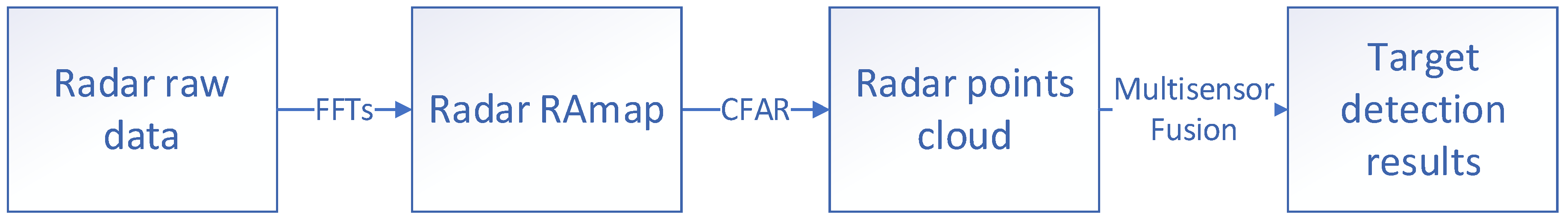
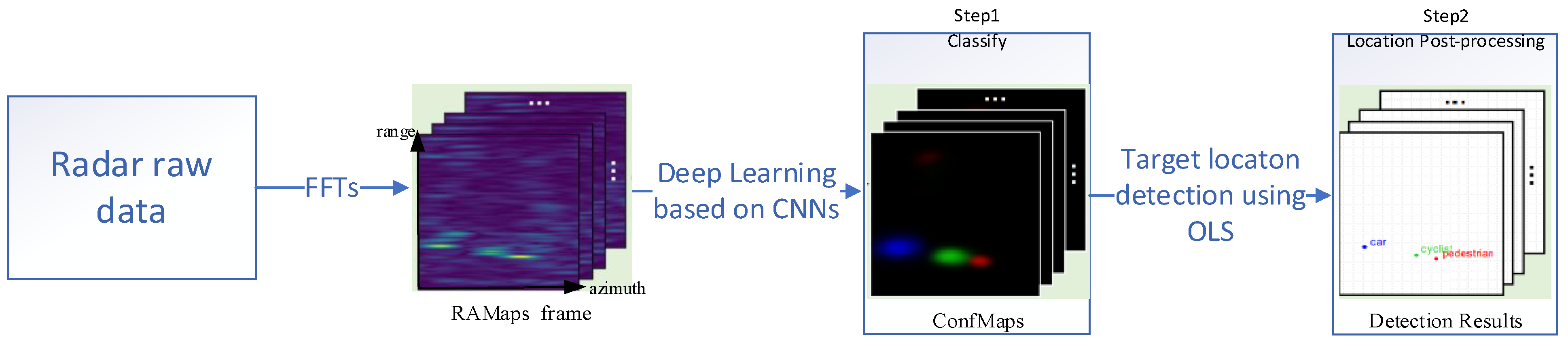
1. Introduction

Millimeter-wave radar is one of the main sensors for vehicle and pedestrian detection in the field of intelligent transportation. Compared with other sensors such as optical cameras and lidars, millimeter-wave radars are more robustly resistant to environmental changes such as different weather and lighting conditions. However, due to the complex scattering effects of clutter, distributed target, and multipath propagation with limited target resolution [1,2,3], it is difficult for millimeter-wave radar data to describe the semantic features of the scene, including the shape of the target, the relationship between targets, etc. The key target-detection problem of millimeter-wave radar is optimizing both false alarm and missed detection [4].

The existing radar data processing flow is mainly as follows. First, the radar raw data are subjected to range and azimuth (RA) Fast Fourier Transform (FFT), and then a Constant False Alarm Rate Detection (CFAR) is performed in the range–azimuth domain data to obtain target point cloud, velocity, and RCS information [5], as shown in Figure 1. Unfortunately, the target-scattering response in nature scenes is more complex than the simplified clutter background model used in CFAR. The local signature of target-scattering response is destroyed after CFAR, which leads to less priori information such as target size and radar measurement accuracy being used to optimize both false alarm and missed detection. Sparser point cloud makes it worse [6].

Recent development of machine-learning techniques, such as CNNs [7,8,9,10,11,12,13,14], enable new methods for radar target detection used in the microwave and optical high-resolution remote-sensing community [15,16,17,18,19,20,21,22,23,24]. Refs. [7,8,9,10,11] highlighted that over recent years, a lot of studies have been published pursuing multi-sensor fusion with various deep convolutional neural networks and obtaining a state-of-the art performance in object detection and recognition. DCNNs were first introduced by K. Fukushima [12], using the concept of a hierarchical representation of receptive fields from the visual cortex, as presented by Hubel and Wiesel. Afterward, Weibel et al. Ref. [13] proposed convolutional neural networks (CNNs) that share weights with temporal receptive fields and Backpropagation training methods. Later, Y. LeCun [14] presented the first CNN architecture for document recognition. The DCNN models typically accept 2D images or sequential data as the input. Based on radar image, Ref. [19] designed an aggregation module to merge the data from all chirps in the same frame to make full use of radar data in object detection and various Gaussian noises with different parameters are employed to increase data diversity and reduce over-fitting based on the analysis of training data. Ref. [20] proposed a novel cross-modality deep-learning framework for the radar object detection task using the Squeeze-and-Excitation network. A novel noise detection approach is also explored in the study to increase the model’s ability to handle noise. Ref. [21] proposed novel scene-aware sequence mix augmentation (SceneMix) and scene-specific post-processing to generate more robust detection results. Ref. [22] proposed a dimension apart network (DANet) for a radar object detection task to be lightweight and capable of extracting temporal–spatial information from the RAMap sequences. Ref. [23] also proposed a lightweight, computationally efficient, and effective network architecture to conquer the question of the trade-off between computational efficiency and performance of radar object-detection tasks. The radar cube is introduced in [24] to maximize the use of radar input data. The aforementioned literature is mainly on the use of data and network lightweight research, but no one has studied improvement methods based on target number.

Spatial bias is a type of inductive bias in CNNs that assumes a certain type of spatial structure present in the data, which can be used to learn the local signature of target-scattering response in the RA image sequence. However, the use of CNNs in low-resolution data such as a Multiple-Input Multiple-Output (MIMO) radar image in the automatic driving scenario presents certain challenges. RODNet firstly introduces CNNs into MIMO radar image feature expression [25]. It uses a chirp-merging module (M-Net), and a temporal deformable convolution (TDC) operation directly learns and encodes the target features from the range–azimuth images to improve the limitation of low resolution MIMO radar image. The M-Net is designed to enhance the SNR of input data using multi-chirp RA images. In addition, the TDC uses the deformable convolution network (DCN) [26] to accomplish the 3D CNN [8,9,27,28] to handle the radar object dynamic motion within the input RA images per frame.

After encoding the multi-chirp RA images for each frame, the RODNet will generate a confidence map (ConfMap) of predicated target locations and classes from the merged image signature codes. The value of ConfMap is assumed to be a Gaussian distribution representing the possibility of point target-detection results occurring at a range–azimuth location. The final detection result is then obtained by the position-processing method. The sorting process is shown in Figure 2. However, RODNet is a cross-supervised training scheme that is characterized by a lack of bounding box. This makes it difficult for RODNet to predict the boundary of the target in the RA coordinate system based on ConfMap. The object-location similarity (OLS) metric, which is like an intersection over union (IoU) [29,30,31,32,33,34,35,36], is proposed to estimate the position of the point target. As it depends only on the sparse high ConfMap value information, the unknown effects on the ConfMap from multi-target, multipath scattering and poor resolution make it difficult to balance the false alarm and missed detection in the dense scenes, as shown in Figure 3. RODNet detects the two proximal pedestrian targets as one because their ConfMaps are overlapped.

The ConfMap of a certain class predicated by CNNs-based RODNet is believed to indicate the probability of target in an RA grid. However, the OLS method ignores the fact that the number of targets is a hidden variable of the target location. This makes the complex scattering of dense scenes affect the distribution of ConfMap values, which in turn affects the accuracy of target number estimation and ultimately leads to errors in target detection. In order to avoid this problem, this paper intends to independently estimate the target number using ConfMap value distribution and estimate target location using the occupied grid spatial distribution of ConfMap. This new algorithm can improve the detection accuracy by correcting the wrong target estimation number.

Overall, our main contributions are the following:

• Based on the actual data, we analyze the characteristics of ConfMap predicated by RODNet and the limitations of the OLS target-location detection method. The relationship among ConfMap value distribution, occupied grid spatial distribution, and target number is analyzed.
• GMM-TN, a target-state likelihood model with ConfMap value for observation is introduced for simulating the conditional ConfMap value and occupied grid spatial distribution with target number as condition.
• The KL distance measure between the predicated ConfMap of RODNet and the simulated ConfMap under the condition of the given target number is derived, and the maximum posteriori target number estimation is constructed. The CRUW dataset is used to verify the improved missed detection and false alarm of the method.

This paper is organized as follows: the relationship between the value of ConfMap, the spatial distribution of occupied grids, and the number of targets is analyzed by actual data in Section 2. Section 3 describes the method of establishing the GMM-TN model and constructs the maximum for a posteriori target number estimation method. In Section 4, the experiment applied to the CRUW dataset scenarios is introduced. Finally, we summarize our algorithm and experiment results.

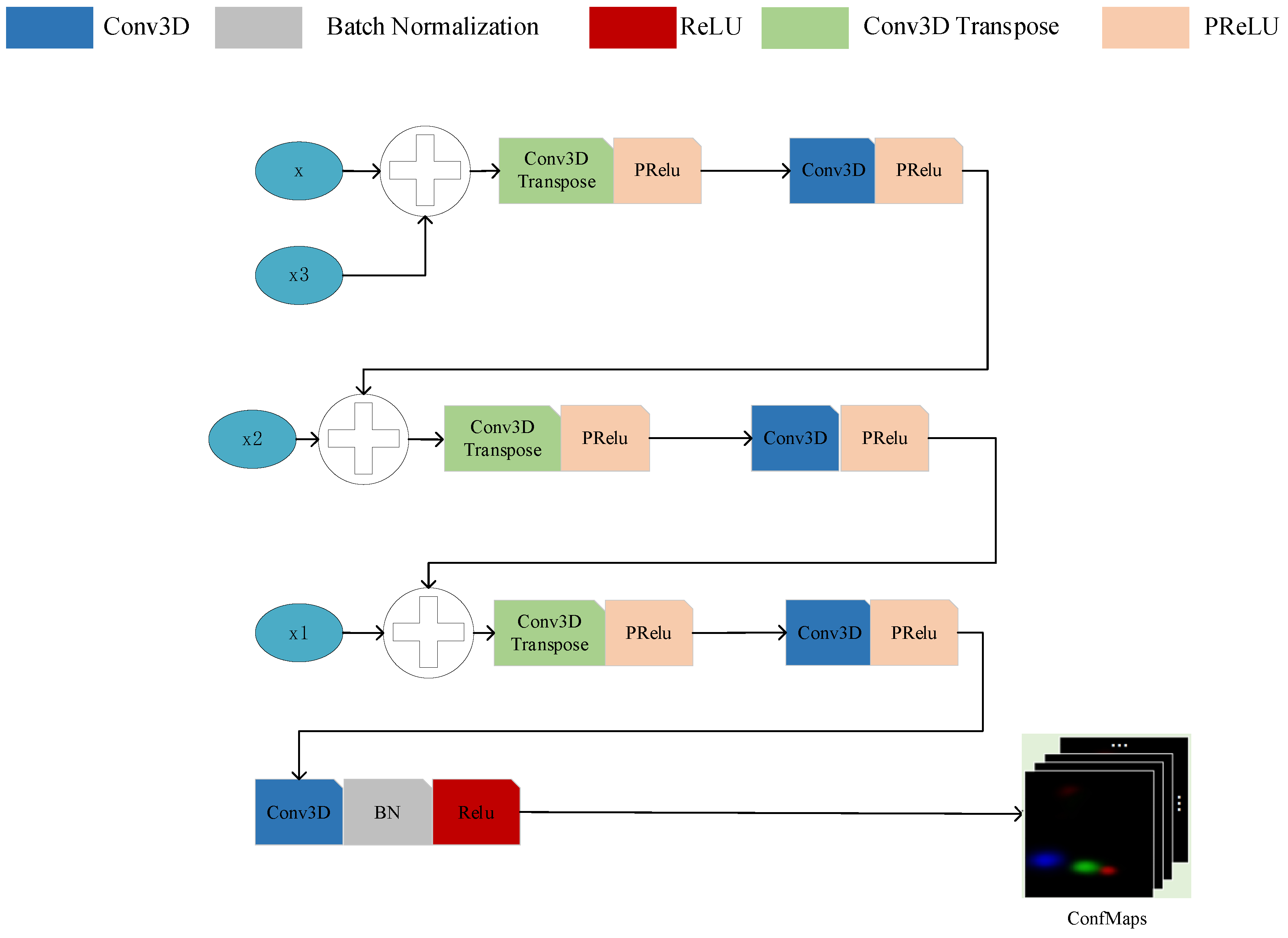
2. RODNet ConfMap Characteristics and Limitations

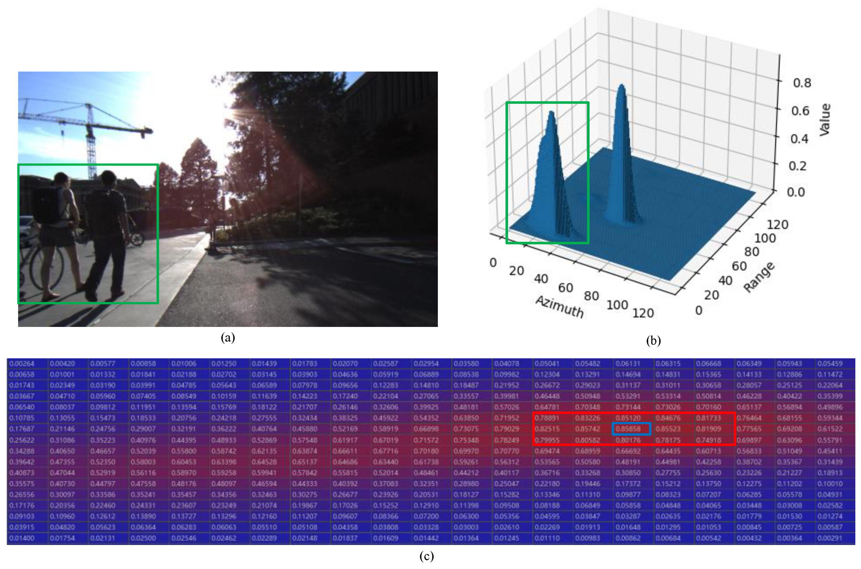
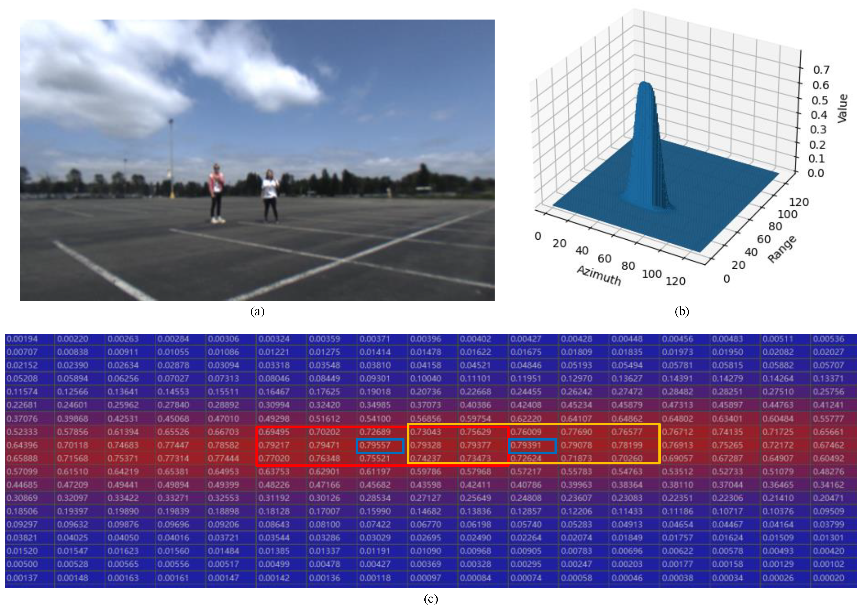
2.1. ConfMap Characteristic Analysis

The RODNet is implemented based on a 3D CNN with an autoencoder architecture. The network architecture first uses some basic three-dimensional convolution structures, then adds a skip connection layer [37] and implements a three-dimensional convolution neural network based on the Hourglass (HG) architecture to ensure that each new convolution operation is not inferior to the previous one. In order to better apply the information contained in all chirps, the author proposes a chirp-merging module (M-NET). Given that the relative motion between the radar and the target causes the radar reflection mode to change with time and the multi-level features are fused, a temporal deformable convolutional (TDC) layer is added to the network [26]. Finally, the network achieved a better classification result. Its encoder and decoder schematic are shown in Figure 4 and Figure 5.

In the decoder shown in Figure 5, we perform feature restoration through deconvolution operations to expand the size of the feature map. At the same time, a convolution operation is performed after each layer of deconvolution, which can effectively extract features while expanding the size of the feature map.

The value of the predicated ConfMap of RODNet can be equivalent to the probability P_cls(r, a) that a specific class cls of target will appear on the grid (r, a). RODNet can detect three classes of targets, namely cars, cyclists, and pedestrians. The three classes of target ConfMaps can be obtained from the three channels of RODNet output after normalized processing. The network framework of RODNet is built based on CNNs. Due to the characteristics of CNNs, the predicated ConfMap of RODNet will have local relevance. Figure 6 is a visual representation of a ConfMap.

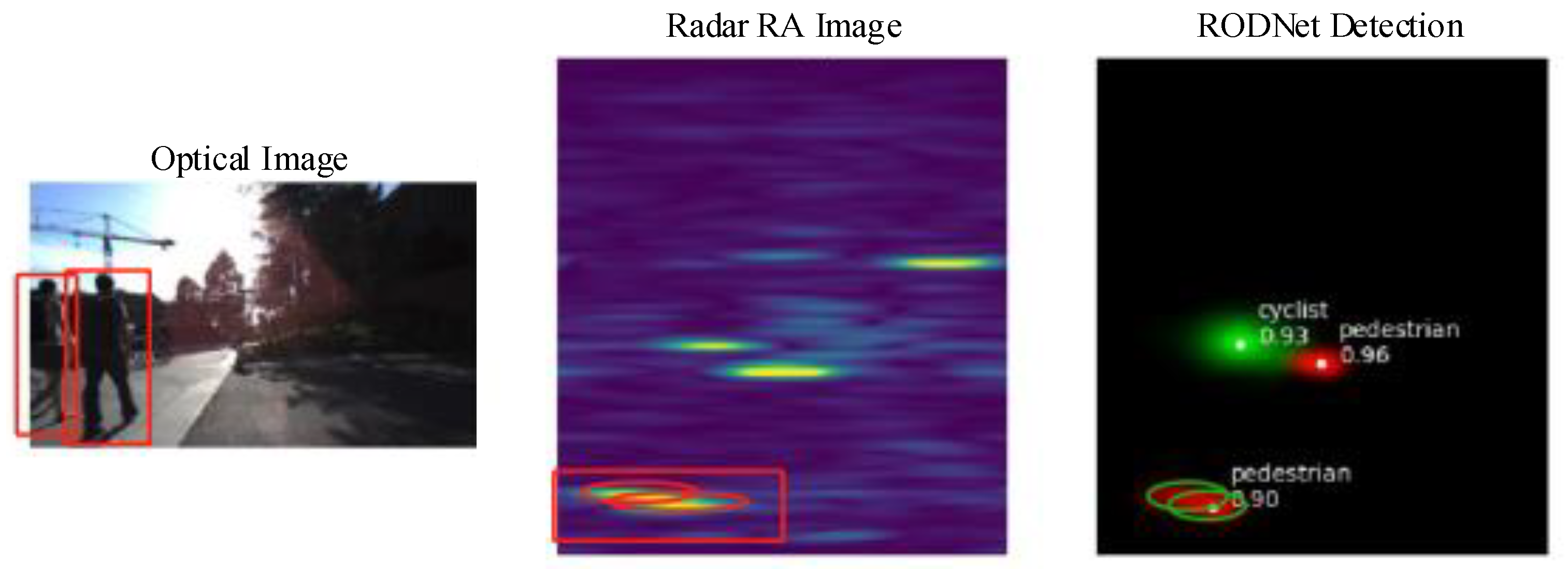
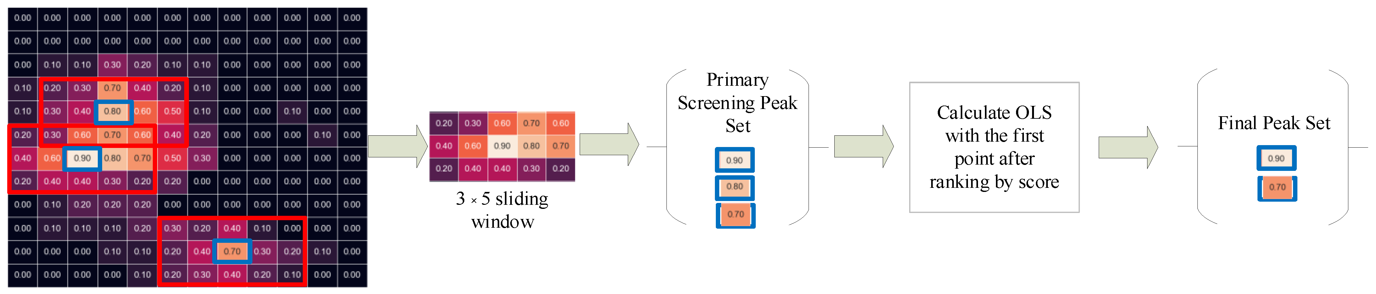
2.2. Object-Location Similarity (OLS) Limitation Analysis

In the process of target-location processing [25], the author proposes a peak detection algorithm. The algorithm traverses ConfMap through a 3 × 5 sliding window and obtains the final location result by filtering the peak and recursively calculating OLS. The flow chart for target-location detection using OLS is shown in Figure 7.

The formula of OLS proposed in [25] is as follows:

$$OLS=\exp \left\{\frac{-d^2}{2{(s\times k_{cls})}^2}\right\}$$

(1)

where d is the distance (in meters) between any two points in a radar RA image; s is the object distance from the radar sensor, representing object scale information; and κ_cls is a per-class constant that represents the error tolerance for class cls, which can be determined by the object average size of the corresponding class. κ_cls is a priori setting such that OLS can be reasonably distributed between 0 and 1.

The OLS can be interpreted as a Gaussian distribution, with distance d as the bias and (s × κ_cls)² as the variance. Therefore, OLS is a similarity measure which also considers object size and distance, so it is more reasonable than other traditional distance measures (such as Euclidean distance, Mahalanobis distance, etc). This OLS metric is also used to match detections and ground truth for evaluation purposes.

According to the OLS target-location detection method, we can infer that the author makes three assumptions as follows:

• Point target hypothesis;
• No point target overlap will occur in ConfMap;
• The value distribution of ConfMap is related to the corresponding probability distribution of point target location and class;
• Considering the above assumptions, there are several typical cases, which can be analyzed as below.

• Case (1): Single target in ConfMap

There is only one target in the ConfMap area, but multiple grids with high probability values appear. In this case, we first need to analyze the reasons for this situation. Because the input of RODNet is radar RA map frames, that is, the original radar data are obtained by FFTs transforms, each frame of the radar RA map is obtained by multiple chirp combinations, and each chirp acquisition is affected by the randomness of radar positioning, that is, the radar accuracy itself is a random quantity, which may cause the process of extracting features in multiple chirp combinations to be extracted into multiple high probability points. In addition, because the target collected by the radar itself should be a distributed target during the acquisition process, the point target assumption is not satisfied, which will result in multiple strong points in the data and eventually be extracted into multiple high probability grids. Finally, the adjacent target may produce a multipath effect, which will also affect the point target hypothesis. The above results in the situation of case (1).

For a single pedestrian target, because such targets are small, the initial screening process can directly obtain the peak value, so the method can obtain good results. Figure 8 shows this case.

• Case (2): No overlapped multiple targets in ConfMap

There are two targets in the region of the ConfMap; they are far apart, and each of the two targets has a peak. The schematic diagram of this case is shown in Figure 9. When the initial screening is completed, two peaks can be obtained. In the process of calculating OLS, the larger the d is, the smaller the exponential part is, and the OLS is closer to 0. This target-location processing method can also give accurate results.

• Case (3): Type 1 overlapped multiple targets in ConfMap

There are two targets in the region of the ConfMap, but there is only one grid with a high probability value. Case (3) is shown in Figure 10. Because only one peak point is retained during the initial screening process, the result is missed.

• Case (4): Type 2 overlapped multiple targets in ConfMap

There are two targets in the region of the ConfMap, but the high probability grid points are close, or even overlap. Case (4) is shown in Figure 11. When two grids with high probability appear at the same time at close range, d will become smaller in OLS calculation, the index part will approach 0, and OLS will become larger. When the threshold is exceeded, another strong point will be suppressed. In this case, OLS will also result in missed detection.

In summary, in cases (1) and (2), the OLS-based location detection method performs well. However, in cases (3) and (4), the method has missed detection and has been verified by measured radar data, confirming the limitations of the method. The reason for case (3) is the missed detection of the sliding window. Furthermore, the reason for case (4) is that the d in Equation (1) is too small, which causes the value of OLS to become larger than the threshold, so one point is wrongly suppressed. We have considered increasing the OLS threshold or modifying the size of the sliding window. Although the former can ensure the adjacent peak point is retained, it may also lead to an error that should be suppressed. The latter situation may cause the peak point to be missed in dense cases (or overlapping). Simple adjustments cannot directly solve the problem, so a new method needs to be proposed. In the next chapter, we will introduce our new method in detail.

3. Dense Target-Location Detection Method Based on Maximum Likelihood Estimation

To solve the problem of missed detection of RODNet, we developed the Gaussian Mixture Model with target number (GMM-TN). It can be considered that this is also a clustering algorithm that automatically detects the best number of overlapping clusters. The K-means algorithm is the part of it which is used only to find the centroids of the assumed cluster number. Then, the Gaussian Mixture Model is used to simulate the ConfMap under this assumption. For each cluster number assumption, the KL distance between the simulated ConfMap and the ConfMap generated by RODNet is calculated. If the KL distance is the shortest, the corresponding cluster number assumption will be considered as the best number of clusters.

3.1. Gaussian Mixture Model with Target Number

The assumptions used in the GMM-TN model are listed as follows:

• Point target hypothesis;
• Point target overlap may occur in ConfMap;
• Both the value distribution and occupied grid spatial distribution of ConfMap are related to the corresponding probability distribution of point target location and class.

The simulated ConfMap $P_{cls}\left(a,r\right)$ can be equivalent to the full probability of occurrence of class cls point targets at grid (a, r) in a 128 × 128 grid image (refer to the radar RA map in Figure 3) is shown in Equation (2).

$$P_{cls}\left(a,r\right)=\frac{1}{B}{\displaystyle \sum _{n=0}^N{P}_{n,cls}\left(a,r\right)}$$

(2)

where a and r are the column index and row index of radar RA map, respectively; B is the normalized coefficient of probability; and N is the number of targets in a single radar RA map. $P_{n,cls}\left(a,r\right)$ is the probability of occurrence of nth point target of class cls at grid (a, r), which is related with several hidden variable conditions and can be rewritten as follows

$$\begin{array}{l}{P}_{n,cls}\left(a,r\right)=P\left(\left(a,r\right)|{\sigma }_{cls},a_0\left(n\right),r_0\left(n\right)\right)\\ =\frac{1}{2\pi }\exp \left\{-\frac{{[(r-r_0\left(n\right))\times 2]}^2+{(a-a_0\left(n\right))}^2]}{2{({\sigma }_{cls})}^2}\right\}\end{array}$$

(3)

$${\sigma }_{cls}=2\arctan (\frac{l_{cls}}{2r})\times c_{cls}$$

(4)

where $r_0\left(n\right)$ and $a_0\left(n\right)$ are the row and column grid index of nth point target, respectively. The condition hidden variable ${\sigma }_{cls}$, as shown in Equation (4), represents the standard deviation of the size of the target in the ConfMap which is approximate to a Gaussian distribution, where l_cls is a class-related prior information, a pedestrian is 1, a cyclist is 2, and a car is 3. c_cls is also priori information. The value of pedestrians is 15, the value of cyclists is 20, and the value of cars is 30. The denominator is multiplied by 2 because the reflection pattern in the radar RA image is usually elliptical.

Considering that the key operation for dense target detection depends mainly on the azimuth resolution ability, we also can use the marginal probability distribution in azimuth direction. The two-dimensional probability density Equation (2) becomes:

$$P_{cls}\left(a\right)=\frac{1}{C}{\displaystyle \sum _{r=1}^{128}{P}_{cls}\left(a,r\right)}$$

(5)

where C is the normalized coefficient of probability.

The overall flow chart is shown in Figure 12. In the classification stage, we make use of exactly the same feature extraction part of RODNet—the network and weights of original RODNet to generate a ConfMap, as shown in Figure 12a. Because the problem we are dealing with is the location processing, our improvements to RODNet are shown in Figure 12b.

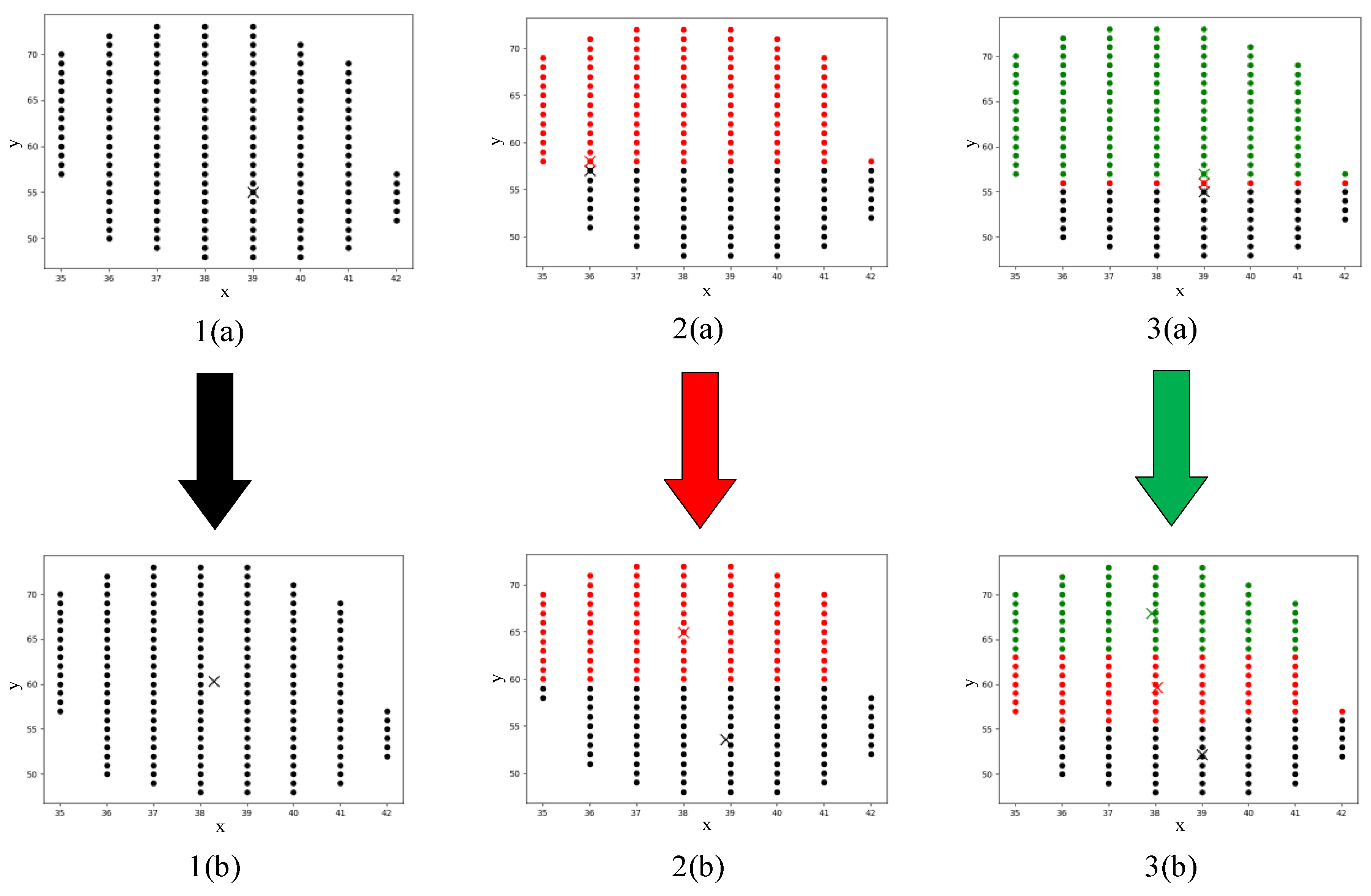
3.2. Target Number Estimation Method

Based on the simulation method mentioned in Section 3.1, we combine clustering and KL distance to construct a set of target number determination methods. We first perform the following operations on the output results with ConfMap:

(1)

Sort the scores of the results;

(2)

Calculate the distance between each coordinate and the highest score coordinate in turn;

(3)

If the threshold is exceeded, the grid coordinate is saved to another list; otherwise, the coordinates and the surrounding area greater than 0.3 enter our algorithm;

(4)

Loop steps (2) and (3) until the last one is over and repeat steps (2) and (3) in the ‘another list’.

Our target-location detection algorithm process is shown in the Figure 13.

The overall process of the method is as follows. First, the ConfMaps output from the RODNet network is extracted. Because the number of targets and the location of point targets are unknown in the ConfMap with overlap, the Maximum A Posteriori parameter estimation framework is constructed by combining the GMM-TN and the predicted ConfMap as a condition to determine the number and location of point targets. Because we aim at the part of the network after the completion of the classification of the ConfMap, no matter how the network structure is designed, this method can ensure that after classification, our target-location detection will improve the accuracy of the results. The subsequent experimental section will involve further discussion of the results.

In order to obtain $r_0\left(n\right)$ and $a_0\left(n\right)$ in Equation (3), we assume each clustering center of a ConfMap occupied grid spatial distribution as the nth point target center with target number as a predefined condition. There are four categories of clustering method: the partition clustering method, the density-based clustering method, the hierarchical clustering method, and the new method. K-means, which is used to perform this operation, is one of the most widely used partition clustering algorithms [38,39]. It should be noted that not only the K-means method but also any clustering algorithm with a pre-defined number of clusters and based on the geometric distance between sample points can be applied to the GMM-TN algorithm to find the clustering centroids.

After determining the target center and the simulation method, it is necessary to measure the difference between two kinds of distribution: one is the normalized ConfMaps predicated by RODNet, expressed by $P_{cls}^{RODNet}\left(a,r\right)$. Another distribution is the simulated ConfMap $P_{cls}\left(a,r\right)$ defined in Equation (2).

KL divergence is a widely used measure of the similarity between two probability distributions. In this paper, the two-dimensional KL divergence is defined as:

$$K{L}_{2D}=D(P_{cls}^{RODNet}\left(a,r\right)||P_{cls}\left(a,r\right))={\displaystyle \sum _{a=1}^{128}{\displaystyle \sum _{r=1}^{128}{P}_{cls}^{RODNet}\left(a,r\right){\log }_2\frac{P_{cls}^{RODNet}\left(a,r\right)}{P_{cls}\left(a,r\right)}}}$$

(6)

As the KL divergence is asymmetric, we can modify Equations (6) to (7):

$$\begin{array}{l}K{L}_{2D}=D(P_{cls}^{RODNet}\left(a,r\right)||P_{cls}\left(a,r\right))+D(P_{cls}\left(a,r\right)||P_{cls}^{RODNet}\left(a,r\right))\\ ={\displaystyle \sum _{a=1}^{128}{\displaystyle \sum _{r=1}^{128}{P}_{cls}^{RODNet}\left(a,r\right){\log }_2\frac{P_{cls}^{RODNet}\left(a,r\right)}{P_{cls}\left(a,r\right)}}}+{\displaystyle \sum _{a=1}^{128}{\displaystyle \sum _{r=1}^{128}{P}_{cls}\left(a,r\right){\log }_2\frac{P_{cls}\left(a,r\right)}{P_{cls}^{RODNet}\left(a,r\right)}}}\end{array}$$

(7)

According to Equation (7), the smaller the $K{L}_{2D}$ is, the smaller two-dimensional probability distribution difference is, and vice versa.

Based on Equation (5), it is reasonable to consider the azimuth-only case; therefore, the one-dimensional KL divergence can be defined as:

$$\begin{array}{l}K{L}_{1D}=D(P_{cls}^{RODNet}\left(a\right)||P_{cls}\left(a\right))+D(P_{cls}\left(a\right)||P_{cls}^{RODNet}\left(a\right))\\ ={\displaystyle \sum _{a=1}^{128}{P}_{cls}^{RODNet}\left(a\right){\log }_2\frac{P_{cls}^{RODNet}\left(a\right)}{P_{cls}\left(a\right)}}+{\displaystyle \sum _{a=1}^{128}{P}_{cls}\left(a\right){\log }_2\frac{P_{cls}\left(a\right)}{P_{cls}^{RODNet}\left(a\right)}}\end{array}$$

(8)

Two maximum likelihood target-number estimation methods are proposed based on two-dimensional and one-dimensional symmetric KL divergence Equations (7) and (8), which are named the 2DMLKL and 1DMLKL method, respectively.

At last, the estimated number of targets with the smallest one-dimensional or two-dimensional symmetric KL divergence can be calculated by Equation (9) or (10):

$$\widehat{N}=\underset{N\in \left\{0,1,\cdots ,N_{\max }\right\}}{\mathrm{Argmin}}K{L}_{1D}$$

(9)

$$\widehat{N}=\underset{N\in \left\{0,1,\cdots ,N_{\max }\right\}}{\mathrm{Argmin}}K{L}_{2D}$$

(10)

where $N_{\max }$ is the predefined maximum possible number of targets in a radar RA image.

The final target number and the corresponding cluster center result are taken as the output, and the probability value corresponding to the cluster center in the predicted ConfMap is taken as the final score.

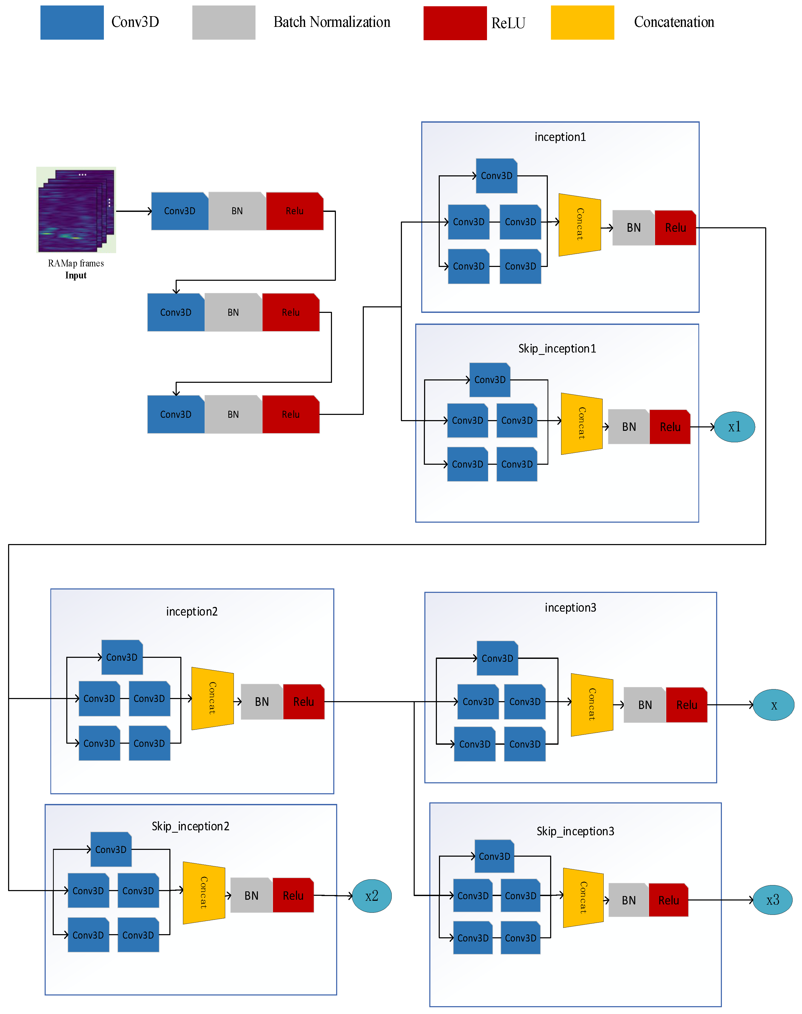
4. Experiments and Analysis

4.1. Experimental Data and Processing Steps

The dataset used in this paper is part of an open-source dataset called Camera-Radar of the University of Washington (CRUW) [40], which uses the format of radar RA images. The sensor platform includes a pair of stereo cameras and a 77 GHz millimeter-wave FMCW radar. The assembled and mounted sensors are well calibrated and synchronized. The stereo camera setup is designed to provide ground truth values for the dataset. The dataset contains over 3 h of 30 FPS (approximately 400 K frames) camera radar data for different driving scenarios, including campus roads, city streets, highways, parking lots, etc. In addition, it also includes several visual failure scenes with very poor image quality, namely darkness, strong light, blur, etc.

For the content of this paper, we reconstruct the CRUW dataset and divide it into two parts: Dense Pedestrian scene (for short DP scene) and Non-Dense Pedestrian scene (for short NDP scene). It should be mentioned that in the original CRUW dataset, the data containing pedestrians accounts for about 50% of the total CRUW. In the data containing pedestrians, the scene with dense pedestrians accounts for about 8%.

The specific experimental arrangements are as follows. First, we trained RODNet. The encoding–decoding structure we use is shown in Figure 4 and Figure 5. RODNet is based on PyTorch [41]. The models are optimized with an Adam optimizer. The network is trained with a batch size of 2 on NVIDIA RTX2080Ti GPU. The initial learning rate was 1 × 10⁻⁵, and the learning rate step was 5. The optimization is set to stop after 100 epochs. Then we select the best model in the training effect and test with target-location detection using OLS, 2DMLKL and 1DMLKL, respectively. Finally, we will show the four typical cases mentioned in Section 2 with typical scene data. The result graph will show the ConfMap results under the assumption of different target numbers simulated by GMM-TN and K-means clustering, and it can be visually compared with the ConfMap predicted by RODNet.

Later, we will introduce the process of our method in detail and show the comparison of the results of target-location detection using OLS and target-location detection using 2DMLKL and 1DMLKL, respectively, for typical scene data. Then, we will compare and verify the difference between the 1DMLKL and 2DMLKL methods and finally give the overall evaluation.

4.2. Typical Sample Results and Analysis

4.2.1. GMM-TN Model Based ConfMap Simulation Results

The process is shown in Figure 13. We take the predicated ConfMap of RODNet as input. For better simulation, we set a threshold of 0.3. The grids with values exceeding the threshold are retained, and those less than the threshold are no longer considered, and the values in these grids less than the threshold are changed to 0. Finally, we normalize the ConfMap after threshold filtering.

Because the value of the ConfMap grid is the probability value that the grid has a target, instead of the probability value that the grid belongs to a certain cluster, it cannot be used as the input of the cluster. Therefore, in the process of clustering, we only consider occupying the grid and use the K-means method to determine the target center. The evolution of clustering iteration is shown in Figure 14.

Using the GNN-TN method mentioned above, we simulate several hypothetical ConfMaps, as shown in Figure 15.

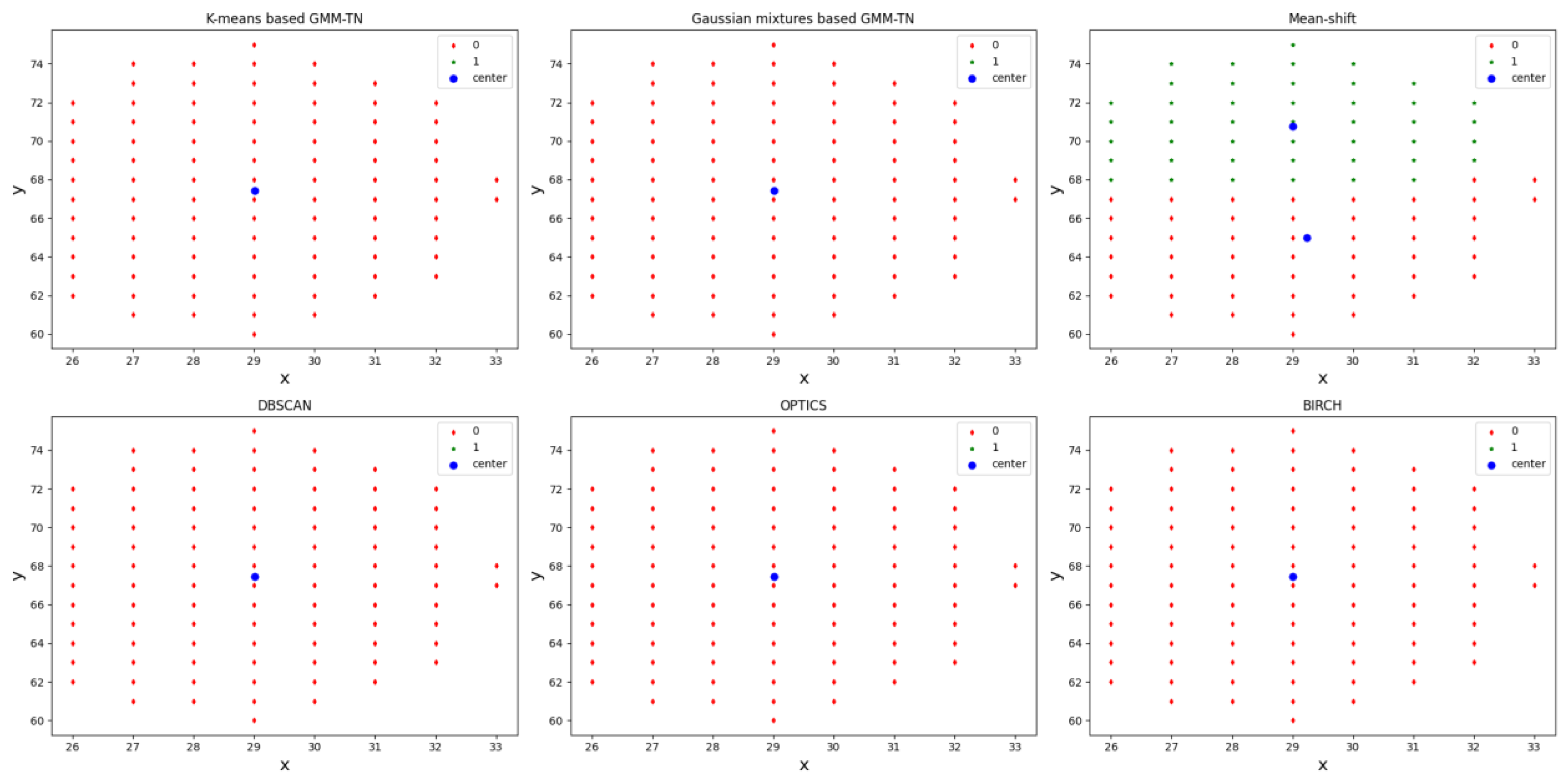
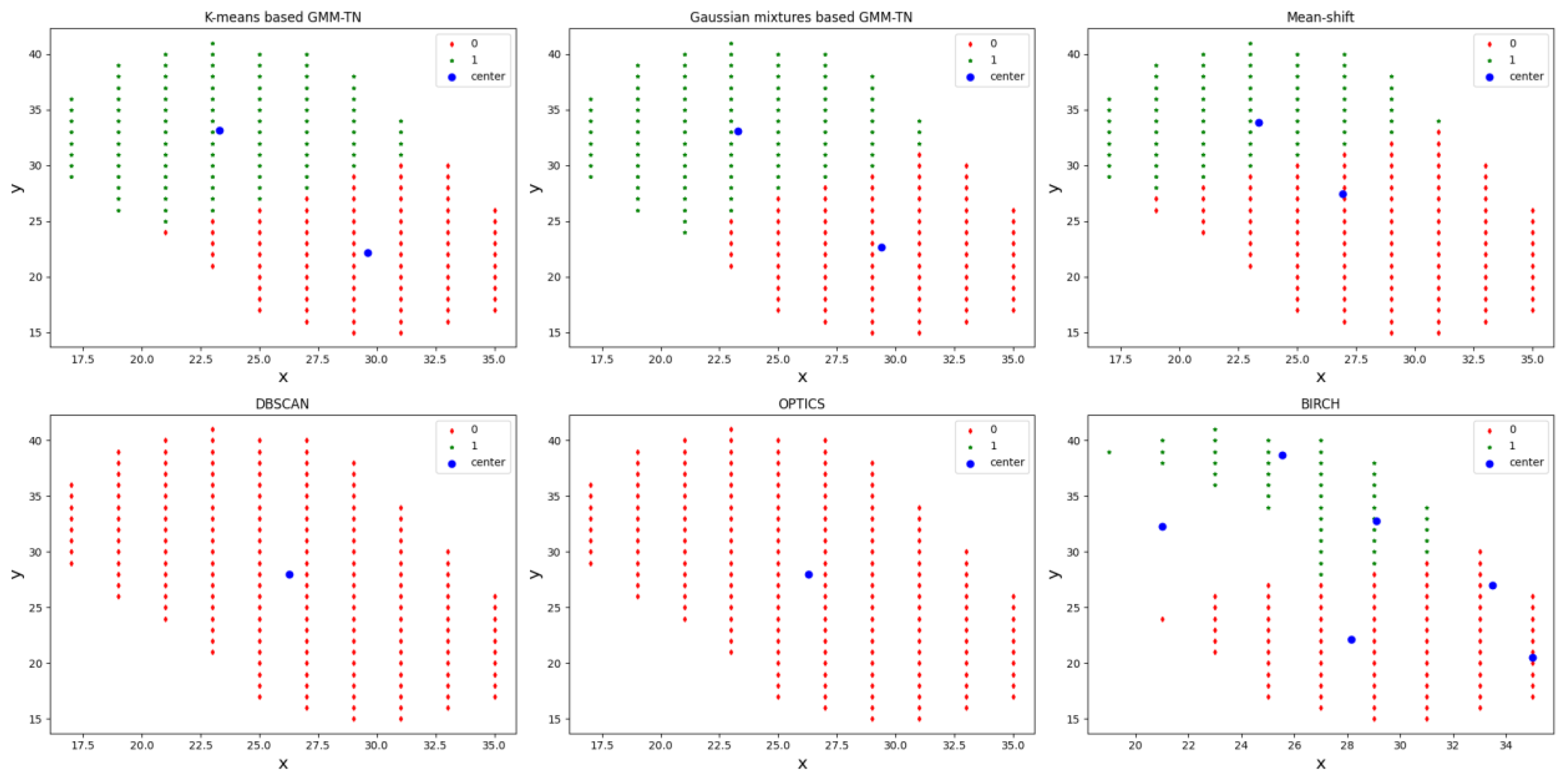
4.2.2. Target Number Estimation Compared with the Other Clustering Methods

The ConfMaps simulated by GMM-TN model are compared with the ConfMap of RODNet by using the KL divergence. It is worth mentioning that because KL divergence > 0, we need to normalize the ConfMaps. Then we are going to calculate the 2DKL divergence using Equation (7) and the 1DKL divergence using Equation (8). After obtaining the corresponding KL divergence value, we use Equations (9) and (10), respectively, to obtain the final number of targets. Then, we output the corresponding position results and scores.

This algorithm is similar to the other clustering algorithms which can find the best number of clusters automatically, such as Mean-shift [42], DBSCAN [39,43], OPTICS [44,45], and BIRCH [46]. Therefore, it is necessary to compare their performance with the GMM-TN algorithm. We randomly take a group of single and double pedestrian data from CRUW for analysis. For the typical single-pedestrian case, the automatic target number estimation results of K-means-based GMM-TN, Gaussian-mixtures-based GMM-TN, Mean-shift, DBSCAN, OP-TICS, and BIRCH are shown in Figure 16. For the double pedestrian case, their responses in ConfMap are overlapped, and their results are shown in Figure 17.

According to the two cases results, we find the GMM-TN algorithm developed in this paper can provide accurate automatic target numbers, either using the K-means or the Gaussian mixtures clustering. Their centroids are somewhat different. However, the Mean-shift and BIRCH algorithms tend to cluster single target into multiple targets, which will lead to a false detection problem. In contrast, the DBSCAN and OPTICS algorithms tend to cluster double targets into single target, which will lead to a missed detection problem.

From the graph signatures of spatial distribution shape, the single target ConfMap generated by RODNet usually satisfies the elliptic hypothesis. For two adjacent targets, their spatial distribution of ConfMap can be modeled as two ellipses overlapping together. We believe that this is related to the FFTs operation used in radar RA map processing and the CNN-based RODNet. This kind of spatial distribution shape feature facilitates clustering methods such as K-means and Gaussian mixtures, which separate samples in n groups of equal variances, minimizing a criterion known as the inertia or within-cluster sum-of-squares. In addition, the KL distance between the simulated ConfMap and the ConfMap generated by RODNet is sensitive to different target number assumptions. However, other clustering algorithms are not directly related to the number of targets but to cluster density or bandwidth.

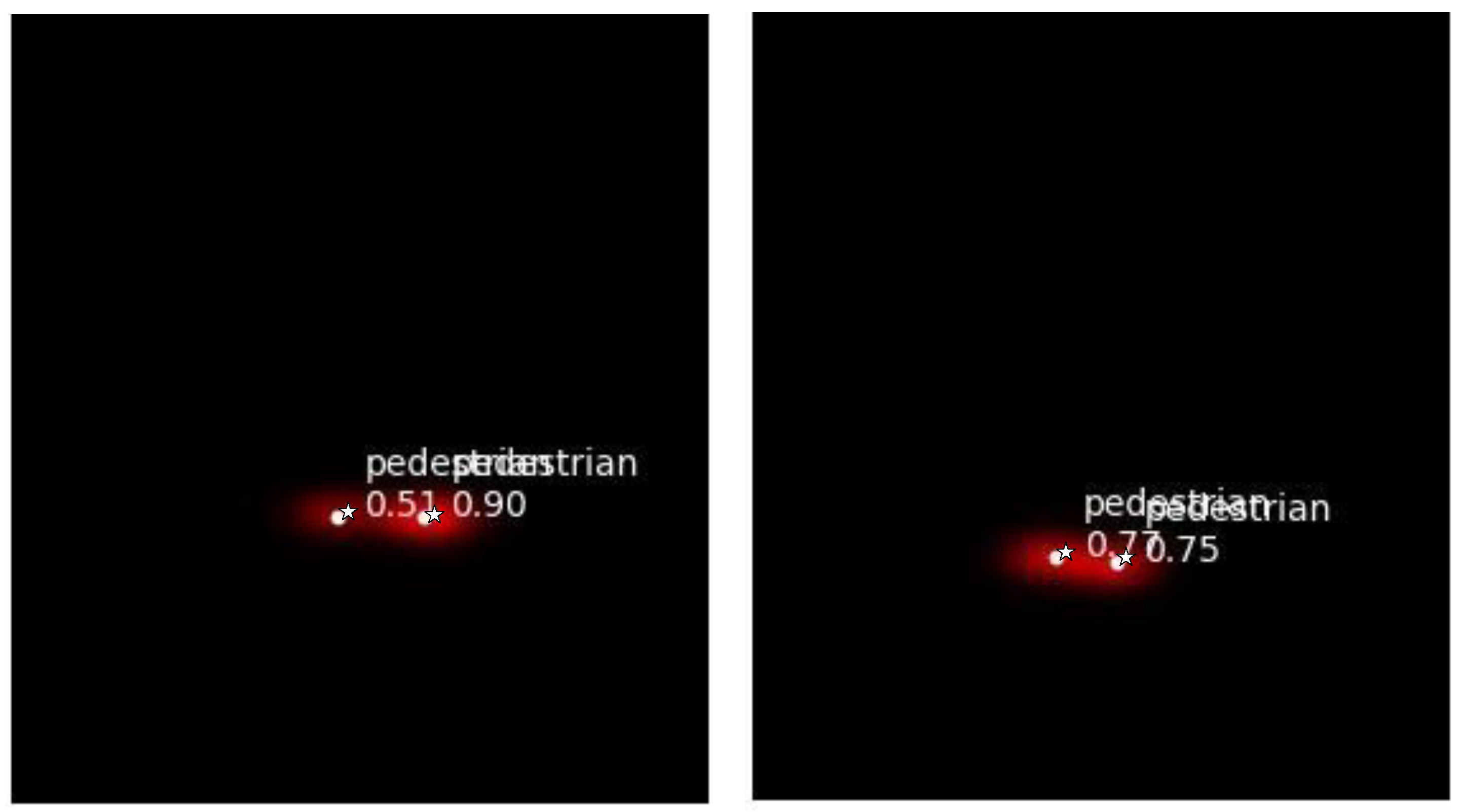
4.2.3. Detection Results Comparison for Dense and Non-Dense Pedestrian Scenes

We experimented with our methods in various typical scenarios and compared it with the RODNet method. The results are shown in Figure 18. The experiment selected typical results for the four cases mentioned above.

In order to ensure that the method mentioned in this paper will not have a negative impact on non-dense target situation, we also conducted experiments on NDP scenes, such as Case (1) and Case (2).

From the diagram, it can be found that for Case (1), both the target-location detection using OLS and using the 2DMLKL (Equation (7)) and 1DMLKL (Equation (8)) methods we proposed perform well. In Case (2), we found that there was a false detection in the detection of 2DMLKL in some frames. The correct number of targets is 2, whereas the number of detected targets is 3. Moreover, the 1DMLKL method accurately detected two targets. For Case (3) and Case (4), both of our methods can detect two dense targets well, whereas the target-location detection using OLS gave an unsatisfactory result.

According to Equations (7) and (8), the larger the assumed target number is, the stronger the corresponding randomness is, which is also confirmed from the results. In addition, because the main influencing factor that makes dense pedestrians unable to be accurately detected is the azimuth axis, the range axis has little effect on the results, so the effect has been improved after using 1DMLKL. In the following paper, we will further use the evaluation indicators to evaluate and analyze the experimental results.

4.3. Statistical Evaluation of Large Amounts of Data

First of all, it is worth mentioning that the author of [25] performed inference and evaluation on the human-annotated data. The quantitative results are shown in

Table 1. Radar object detection performance evaluated on CRUW dataset.

Methods	AP	AR
Decision Tree [6]	4.70	44.26
CFAR+ResNet [47]	40.49	60.56
CFAR+VGG-16 [6]	40.73	72.88
RODNet [25]	85.98	87.86

. The RODNet results are compared with the following baselines that also use radar-only inputs: (1) a decision tree uses some handcrafted features from radar data [6]; (2) CFAR detection is first implemented, and a radar object classification network with ResNet backbone [47] is appended; and (3) similar to (2), a radar object classification network with VGG-16 backbone based on CFAR detections is mentioned in [6]. Therefore, we make use of exactly the same network and weights of original RODNet to generate ConfMap.

Because this article is derived from the optimization of the dense pedestrian situation of RODNet, we use the original evaluation method, that is, OLS as an indicator to calculate the average precision (AP) and average recall (AR). The formula of OLS is Equation (1). AP and AR correspond to Equations (11) and (12). Here, true positive (TP) represents correctly located and classified instances, false positive (FP) represents the false alarm, and false negative (FN) represents the missed detection and/or incorrectly classified instance.

$$Precision=\frac{TP}{TP+FP}$$

(11)

$$Recall=\frac{TP}{TP+FN}$$

(12)

We first calculate OLS between each detection result and ground truth in every frame. Then, we use different thresholds from 0.5 to 0.9 with a step of 0.05 for OLS and calculate the AP and AR for different OLS thresholds, which represent different localization error tolerance for the detection results. Here, we use AP and AR to represent the average values among all different OLS thresholds from 0.5 to 0.9 and use AP^OLS and AR^OLS to represent the values at a certain OLS threshold. Overall, we use AP and AR as our main evaluation metrics for the radar object detection task, which is the same as the original.

Here are some comparison results in

Table 2. Comparison of the results of the method proposed in this paper with those in the original paper.

Scene	Evaluation Index	RODNet	ROD-2DMLKL	ROD-1DMLKL
Dense pedestrian	AP	55.70%	80.62%	84.59%
	AR	52.27%	83.33%	88.28%
Non-dense pedestrian	AP	93.43%	87.98%	92.68%
	AR	94.72%	88.47%	93.32%

.

Through Table 2, we can find that under the new position processing method proposed in this paper, the detection effect of RODNet in the case of the DP scene has been significantly improved, but for the NDP scene, there are some declines. After the distance direction is compressed into one dimension, the two scenes are further improved, and the scene for NDP is also similar to the original method.

We analyze the reason why our method causes the decrease of AP and AR in NDP scenes. As shown in Figure 19, in the radar RA images, the target position in the label is in the upper right part of the ‘ellipse’, as shown by the star in the Figure 19, and the target center we obtain by clustering is in the positive center of the ‘ellipse’. In the CRUW dataset, the author only introduces the CRF (camera–radar fusion) method, which is annotated by the fusion of optical detection projection and radar peak point, without revealing more details. The label may have an error with the actual position. In addition, OLS is also applied to the evaluation process. Target number estimation and position estimation give the evaluation results at the same time and are not carried out separately. Therefore, we consider adding ‘target number accuracy’ (for short TNA) as another evaluation.

We count the number of targets in the detection results of the three methods, and the results are shown in

Table 3. Comparison of the TNA of the method proposed in this paper with those in the original paper.

Scene	Evaluation Index	RODNet	ROD-2DMLKL	ROD-1DMLKL
Dense pedestrian	TNA	52.63%	89.73%	96.21%
Non-dense pedestrian		89.70%	90.62%	95.59%

. The statistical method of TNA is as follows: the ratio of the number of frames correctly estimated by the target number to the number of frames in the total dataset, which is shown as Equation (13), where t is the number of true frames and a is the number of all frames.

$$TNA=\frac{t}{a}$$

(13)

From Table 3, we can conclude that the method proposed in this paper has significantly improved the estimation of the number of targets.

5. Conclusions

Aiming at the problem of missed detection of RODNet in dense pedestrian scenes, this paper proposes an improved method of a RODNet radar target-detection algorithm applied to dense pedestrian scenes. Firstly, we analyze ConfMap predicted by RODNet and the limitations of the OLS target-location detection method. The relationship between ConfMap value distribution, occupied grid spatial distribution, and target number is analyzed as well. Secondly, we propose a target state likelihood model called GMM-TN, which uses ConfMap value for observation to simulate the conditional ConfMap value and occupied grid spatial distribution with the target number as a condition. Finally, we propose a maximum posteriori target number estimation based on KL divergence to obtain a new number of targets. Then the CRUW dataset is used to verify the improved missed detection and false alarm of the method.

Because we focus on dense pedestrian scenes, we reconstruct the CRUW dataset into Dense Pedestrian (DP) scenes and Non-dense Pedestrian (NDP) scenes and design experiments. We used the evaluation indicators AP and AR in RODNet for evaluation and introduced a new indicator target-number accuracy rate to verify the method. The validity of the three main contributions in this paper is verified by analysis. The missed detection of DP scenes has been significantly improved, and our method also shows good robustness in NDP scenes.

However, the feature extraction part of RODNet has not been improved. The method proposed in this paper proves that ConfMap has the potential to provide more information. In the subsequent research, we consider trying a new architecture and using the subsequent information to optimize the previous feature extraction network. At the same time, this paper verifies that this method can obtain an accurate number of targets, but because the original dataset does not give a calibration method, the position estimation method cannot judge whether it is accurate or not. In the future, we will consider evaluating the performance of position detection results by projecting the detection results into optical images.

References

- de Ponte Müller, F. Survey on ranging sensors and cooperative techniques for relative positioning of vehicles. Sensors 2017, 17, 271. [Google Scholar] [CrossRef] [PubMed] [Green Version]
- Yoneda, K.; Suganuma, N.; Yanase, R.; Aldibaja, M. Automated driving recognition technologies for adverse weather conditions. Iatss Res. 2019, 43, 253–262. [Google Scholar] [CrossRef]
- Schneider, M. Automotive radar-status and trends. In Proceedings of the German Microwave Conference, Ulm, Germany, 5–7 April 2005; pp. 144–147. [Google Scholar]
- Nabati, R.; Qi, H. CenterFusion: Center-based Radar and Camera Fusion for 3D Object Detection. In Proceedings of the IEEE/CVF Winter Conference on Applications of Computer Vision, Waikoloa, HI, USA, 5–9 January 2021; pp. 1527–1536. [Google Scholar]
- Richards, M.A. Fundamentals of Radar Signal Processing; Tata McGraw-Hill Education: New Delhi, India, 2005. [Google Scholar]
- Gao, X.; Xing, G.; Roy, S.; Liu, H. Experiments with mmwave automotive radar test-bed. In Proceedings of the 2019 53rd Asilomar Conference on Signals, Systems, and Computers, Pacific Grove, CA, USA, 3–6 November 2019. [Google Scholar]
- Chen, X.; Ma, H.; Wan, J.; Li, B.; Xia, T. Multi-view 3d object detection network for autonomous driving. In Proceedings of the IEEE conference on Computer Vision and Pattern Recognition, Honolulu, HI, USA, 21–26 July 2017; pp. 1907–1915. [Google Scholar]
- Du, X.; Ang, M.H.; Karaman, S.; Rus, D. A general pipeline for 3d detection of vehicles. In Proceedings of the 2018 IEEE International Conference on Robotics and Automation (ICRA), Brisbane, QLD, Australia, 21–25 May 2018; pp. 3194–3200. [Google Scholar]
- Liang, M.; Yang, B.; Wang, S.; Urtasun, R. Deep continuous fusion for multi-sensor 3d object detection. In Proceedings of the European Conference on Computer Vision (ECCV), Lecture Notes in Computer Science, Munich, Germany, 8–14 September 2018; Springer: Cham, Switzerland, 2018; Volume 11220, pp. 641–656. [Google Scholar]
- Ku, J.; Mozifian, M.; Lee, J.; Harakeh, A.; Waslander, S.L. Joint 3d proposal generation and object detection from view aggregation. In Proceedings of the 2018 IEEE/RSJ International Conference on Intelligent Robots and Systems (IROS), Madrid, Spain, 1–5 October 2018; pp. 1–8. [Google Scholar]
- Qi, C.; Liu, W.; Wu, C.; Su, H.; Guibas, L. Frustum PointNets for 3D Object Detection from RGB-D Data. In Proceedings of the IEEE/CVF Conference on Computer Vision and Pattern Recognition, Salt Lake City, UT, USA, 18–22 June 2018; pp. 918–927. [Google Scholar]
- Fukushima, K. A self-organizing neural network model for a mechanism of pattern recognition unaffected by shift in position. Biol. Cybern. 1980, 36, 193–202. [Google Scholar] [CrossRef] [PubMed]
- Waibel, A.; Hanazawa, T.; Hinton, G.; Shikano, K.; Lang, K.J. Phoneme recognition using time-delay neural networks. IEEE Trans. Acoust. Speech Signal Process. 1989, 37, 328–339. [Google Scholar] [CrossRef]
- LeCun, Y.; Bottou, L.; Bengio, Y.; Haffner, P. Gradient-based learning applied to document recognition. Proc. IEEE 1998, 86, 2278–2324. [Google Scholar] [CrossRef] [Green Version]
- Danzer, A.; Griebel, T.; Bach, M.; Dietmayer, K. 2d car detection in radar data with pointnets. In Proceedings of the 2019 IEEE Intelligent Transportation Systems Conference (ITSC), Auckland, New Zealand, 27–30 October 2019; pp. 61–66. [Google Scholar]
- Wang, L.; Tang, J.; Liao, Q. A study on radar target detection based on deep neural networks. IEEE Sens. Lett. 2019, 3, 1–4. [Google Scholar] [CrossRef]
- Nabati, R.; Qi, H. Rrpn: Radar region proposal network for object detection in autonomous vehicles. In Proceedings of the 2019 IEEE International Conference on Image Processing (ICIP), Taipei, Taiwan, 22–25 September 2019; pp. 3093–3097. [Google Scholar]
- John, V.; Nithilan, M.; Mita, S.; Tehrani, H.; Sudheesh, R.; Lalu, P. So-net: Joint semantic segmentation and obstacle detection using deep fusion of monocular camera and radar. In Proceedings of the Pacific-Rim Symposium on Image and Video Technology, Image and Video Technology, PSIVT 2019, Sydney, Australia, 18–22 September 2019; Springer: Cham, Switzerland, 2020; Volume 11994, pp. 138–148. [Google Scholar]
- Yu, J.; Hao, X.; Gao, X.; Sun, Q.; Liu, Y.; Chang, P.; Zhang, Z.; Gao, F.; Shuang, F. Radar Object Detection Using Data Merging, Enhancement and Fusion. In Proceedings of the 2021 International Conference on Multimedia Retrieval (ICMR ’21), Taipei, Taiwan, 21 August 2021; Association for Computing Machinery: New York, NY, USA, 2021; pp. 566–572. [Google Scholar]
- Sun, P.; Niu, X.; Sun, P.; Xu, K. Squeeze-and-Excitation network-Based Radar Object Detection With Weighted Location Fusion. In Proceedings of the 2021 International Conference on Multimedia Retrieval (ICMR ’21), Taipei, Taiwan, 21 August 2021; Association for Computing Machinery: New York, NY, USA, 2021; pp. 545–552. [Google Scholar]
- Zheng, Z.; Yue, X.; Keutzer, K.; Vincentelli, A.S. Scene-aware Learning Network for Radar Object Detection. In Proceedings of the 2021 International Conference on Multimedia Retrieval (ICMR ’21), Taipei, Taiwan, 21 August 2021; Association for Computing Machinery: New York, NY, USA, 2021; pp. 573–579. [Google Scholar]
- Ju, B.; Yang, W.; Jia, J.; Ye, X.; Chen, Q.; Tan, X.; Sun, H.; Shi, Y.; Ding, E. DANet: Dimension Apart Network for Radar Object Detection. In Proceedings of the 2021 International Conference on Multimedia Retrieval (ICMR ’21), Taipei, Taiwan, 21 August 2021; Association for Computing Machinery: New York, NY, USA, 2021; pp. 533–539. [Google Scholar]
- Hsu, C.-C.; Lee, C.; Chen, L.; Hung, M.-K.; Lin, Y.-L.; Wang, X.-Y. Efficient-ROD: Efficient Radar Object Detection based on Densely Connected Residual Network. In Proceedings of the 2021 International Conference on Multimedia Retrieval (ICMR ’21), Taipei, Taiwan, 21 August 2021; Association for Computing Machinery: New York, NY, USA, 2021; pp. 526–532. [Google Scholar]
- Gao, X.; Xing, G.; Roy, S.; Liu, H. RAMP-CNN: A Novel Neural Network for Enhanced Automotive Radar Object Recognition. IEEE Sens. J. 2021, 21, 5119–5132. [Google Scholar] [CrossRef]
- Wang, Y.; Jiang, Z.; Gao, X.; Hwang, J.-N.; Xing, G.; Liu, H. RODNet: Object Detection under Severe Conditions Using Vision-Radio Cross-Modal Supervision. arXiv 2020, arXiv:2003.01816. [Google Scholar]
- Dai, J.; Qi, H.; Xiong, Y.; Li, Y.; Zhang, G.; Hu, H.; Wei, Y. Deformable convolutional networks. In Proceedings of the IEEE International Conference on Computer Vision, Venice, Italy, 22–29 October 2017; pp. 764–773. [Google Scholar]
- Guo, W.; Wang, J.; Wang, S. Deep multimodal representation learning: A survey. IEEE Access 2019, 7, 63373–63394. [Google Scholar] [CrossRef]
- Ren, S.; He, K.; Girshick, R.; Sun, J. Faster R-CNN: Towards real-time object detection with region proposal networks. IEEE Trans. Pattern Anal. Mach. Intell. 2016, 39, 1137–1149. [Google Scholar] [CrossRef] [PubMed] [Green Version]
- Urmson, C.; Anhalt, J.; Bagnell, D.; Baker, C.; Bittner, R.; Clark, M.; Dolan, J.; Duggins, D.; Galatali, T.; Geyer, C. Autonomous driving in urban environments: Boss and the urban challenge. J. Field Robot. 2008, 25, 425–466. [Google Scholar] [CrossRef]
- Van Brummelen, J.; O’Brien, M.; Gruyer, D.; Najjaran, H. Autonomous vehicle perception: The technology of today and tomorrow. Transp. Res. Part C Emerg. Technol. 2018, 89, 384–406. [Google Scholar] [CrossRef]
- Giacalone, J.-P.; Bourgeois, L.; Ancora, A. Challenges in aggregation of heterogeneous sensors for Autonomous Driving Systems. In Proceedings of the 2019 IEEE Sensors Applications Symposium (SAS), Sophia Antipolis, France, 11–13 March 2019; pp. 1–5. [Google Scholar]
- LeCun, Y.; Bengio, Y.; Hinton, G. Deep learning. Nature 2015, 52, 436–444. [Google Scholar] [CrossRef] [PubMed]
- Rashinkar, P.; Krushnasamy, V. An overview of data fusion techniques. In Proceedings of the 2017 International Conference on Innovative Mechanisms for Industry Applications (ICIMIA), Bangalore, India, 21–23 February 2017; pp. 694–697. [Google Scholar]
- Fung, M.L.; Chen, M.Z.; Chen, Y.H. Sensor fusion: A review of methods and applications. In Proceedings of the 2017 29th Chinese Control and Decision Conference (CCDC), Chongqing, China, 28–30 May 2017; pp. 3853–3860. [Google Scholar]
- Fayyad, J.; Jaradat, M.A.; Gruyer, D.; Najjaran, H. Deep learning sensor fusion for autonomous vehicle perception and localization: A review. Sensors 2020, 20, 4220. [Google Scholar] [CrossRef] [PubMed]
- Bombini, L.; Cerri, P.; Medici, P.; Alessandretti, G. Radar-vision fusion for vehicle detection. In Proceedings of the International Workshop on Intelligent Transportation, Hamburg, Germany, 14–15 May 2006; pp. 65–70. [Google Scholar]
- Newell, A.; Yang, K.; Deng, J. Stacked hourglass networks for human pose estimation. In Proceedings of the European Conference on Computer Vision, Venice, Italy, 22–29 October 2017; Springer: Berlin/Heidelberg, Germany, 2016; pp. 483–499. [Google Scholar]
- MacQueen, J. Some methods for classification and analysis of multivariate observation. In Proceedings of the 5th Berkeley Symposium on Mathematical Statistics and Probability, Los Angelas, CA, USA, 18–21 July 1965; University of California: Los Angeles, CA, USA, 1967; pp. 281–297. [Google Scholar]
- Ester, M.; Kriegel, H.P.; Sander, J.; Xu, X. A density-based algorithm for discovering clusters in large spatial databases with noise. In Proceedings of the Second International Conference on Knowledge Discovery and Data Mining, Portland, Oregon, 2–4 August 1996; pp. 226–231. [Google Scholar]
- Wang, Y.; Wang, G.; Hsu, H.M.; Liu, H.; Hwang, J.N. Rethinking of Radar’s Role: A Camera-Radar Dataset and Systematic Annotator via Coordinate Alignment. In Proceedings of the IEEE/CVF Conference on Computer Vision and Pattern Recognition, Nashville, TN, USA, 20–25 June 2021. [Google Scholar]
- Paszke, A.; Gross, S.; Massa, F.; Lerer, A.; Bradbury, J.; Chanan, G.; Killeen, T.; Lin, Z.; Gimelshein, N.; Antiga, L. Pytorch: An imperative style, high-performance deep learning library. arXiv 2019, arXiv:1912.01703. [Google Scholar]
- Comaniciu, D.; Meer, P. Mean Shift: A robust approach toward feature space analysis. IEEE Trans. Pattern Anal. Mach. Intell. 2002, 24, 603–619. [Google Scholar] [CrossRef] [Green Version]
- Schubert, E.; Sander, J.; Ester, M.; Kriegel, H.P.; Xu, X. DBSCAN revisited, revisited: Why and how you should (still) use DBSCAN. ACM Trans. Database Syst. 2017, 42, 19. [Google Scholar] [CrossRef]
- Ankerst, M.; Breunig, M.M.; Kriegel, H.P.; Sander, J. OPTICS: Ordering points to identify the clustering structure. ACM Sigmod Rec. 1999, 28, 49–60. [Google Scholar] [CrossRef]
- Schubert, E.; Gertz, M. Improving the Cluster Structure Extracted from OPTICS Plots. In Proceedings of the LWDA 2018: Conference “Lernen, Wissen, Daten, Analysen”, Mannheim, Germany, 22–24 August 2018; pp. 318–329. [Google Scholar]
- Tian, Z.; Ramakrishnan, R. Miron Livny: BIRCH: An Efficient Data Clustering Method for Very Large Databases. ACM Sigmod Rec. 1999, 25, 103–114. [Google Scholar]
- Angelov, A.; Robertson, A.; Murray-Smith, R.; Fioranelli, F. Practical classification of different moving targets using automotive radar and deep neural networks. IET Radar Sonar Navig. 2018, 12, 1082–1089. [Google Scholar] [CrossRef]