Artificial Neural Networking Magnification for Heat Transfer Coefficient in Convective Non-Newtonian Fluid with Thermal Radiations and Heat Generation Effects

Abstract

In this study, the Casson fluid flow through an inclined, stretching cylindrical surface is considered. The flow field is manifested with pertinent physical effects, namely heat generation, viscous dissipation, thermal radiations, stagnation point flow, variable thermal conductivity, a magnetic field, and mixed convection. In addition, the flow field is formulated mathematically. The shooting scheme is used to obtain the numerical data of the heat transfer coefficient at the cylindrical surface. Further, for comparative analysis, three different thermal flow regimes are considered. In order to obtain a better estimation of the heat transfer coefficient, three corresponding artificial neural networks (ANN) models were constructed by utilizing Tan-Sig and Purelin transfer functions. It was observed that the heat transfer rate exhibits an inciting nature for the Eckert and Prandtl numbers, curvature, and heat generation parameters, while the Casson fluid parameter, temperature-dependent thermal conductivity, and radiation parameter behave oppositely. The present ANN estimation will be helpful for studies related to thermal energy storage that have Nusselt number involvements.

1. Introduction

It is a well-known fact among researchers that the study of heat transfer has numerous applications, such as in combustion chambers, furnaces, individual nuclear reactors, heat exchangers with high temperatures, and recuperating thermal energy storage systems, to name just a few. In this regard, the heat transfer coefficient, namely the Nusselt number, contributed to a better heat exchange rate. Due to this motivation, various researchers investigate the heat transfer aspects of the Casson fluid model [1], such as Casson fluid flow in the vicinity of a stagnation point in the direction of a stretched sheet as described by Meraj et al. in [2]. The analysis is also done on the properties of heat transmission with viscous dissipation. In addition, through appropriate transformations, the equations describing heat transport in Casson fluid were reduced. The Casson fluid, velocity ratio parameters, Prandtl and Eckert numbers were the factors controlling the flow. The homotopy analysis method (HAM) was used to calculate the analytical solutions across the entire geographical domain. The Nusselt number and the skin friction coefficient were computed and analyzed. The heat transfer in Casson fluid flow across a nonlinearly extending surface was investigated by Swati [3]. The momentum and energy equations were transformed into reduced equations by utilizing the appropriate transformations. Further, with the aid of the shooting approach, numerical solutions were obtained. The velocity field was suppressed while temperature increased toward the Casson parameter. The heat transmission in a Casson fluid past a symmetric wedge with mixed convection was examined by Swati et al. [4]. The graphical representations of a representative collection of graphic outcomes were produced by the shooting method. It was discovered that while the temperature fell with a higher Falkner-Skan exponent, the velocity increased. Although the temperature was observed to drop in this situation. The temperature is found to decrease as the Prandtl number rises. Pramanik [5] looked into the boundary layer flow of Casson fluid combined with heat transfer in the presence of suction or blowing at the surface toward an exponentially extending surface. The equation for the temperature field included a factor for thermal radiation. The momentum and heat transmission equations were reduced by using suitable transformations. Then, numerical answers to these equations were discovered. Both velocity and temperature show an opposite nature toward the Casson fluid parameter. The temperature rises as a result of thermal radiation, which improves effective thermal diffusivity. Mahdy [6] offered numerical solutions for heat transfer in Casson fluid past a cylinder. Additionally, by using similarity transformations, the controlling partial differential equations were reduced to ordinary differential equations, and the resulting equations were then numerically solved using the shooting method. The primary goal was to look into how the governing variables affected the velocity, temperature profiles, skin friction coefficient, and temperature gradient at the surface.

In an unstable flow of a Casson fluid approaching a stagnation point across a stretching/shrinking sheet in the presence of thermal radiation, Abbas et al. [7] provided the heat and mass transfer study for Casson fluid. They took into account the linear Rosseland approximation for thermal radiation. In considering chemical reactions as a function of temperature, the influence of binary chemical reactions with Arrhenius activation energy was also taken into account. The bivariate spectral collocation quasi-linearization approach was used to produce the numerical solutions of the system of nonlinear PDEs that are constant throughout the entire domain and at all times. Subsequently, the numerical results for a number of relevant physical parameters were visually discussed as fields of velocity, temperature, and concentration. A moving wedge containing gyrotactic microorganisms was the subject of the study by Raju et al. [8] on the effects of thermophoresis and Brownian motion on two-dimensional magnetohydrodynamics (MHD) radiative Casson fluid. Using Runge-Kutta and Newton’s methods, numerical results were presented graphically as well as in tabular form. In the two flow instances of suction and injection, the effects of pertinent parameters on the distributions of velocity, temperature, concentration, and density of motile organisms were given and addressed. Further, in comparing the obtained results to the existing prior studies, the results were validated and determined to be in good agreement. The temperature and concentration field are increased as the thermophoresis parameter values rise. The fact that gyrotactic microorganisms can speed up mass and heat transfer rates was a significant discovery of the present study. Reddy et al. [9] examined the consequences of conjugate heat transfer (CHT) on the idea of a heat function. The Casson fluid was physically represented as it passed through a thin, vertical cylinder. The hollow cylinder’s inner wall was kept at a constant temperature. Additionally, by using an implicit methodology, the solutions to the linked, non-linear governing equations are discovered. All of the governing parameters were shown graphically in the flow charts. The Casson fluid parameters’ steady-state times were prolonged. The heat function contours were concentrated near the leading edge at the cylinder’s hotter wall. Furthermore, by increasing the values of all the regulating parameters, the heat lines’ departures from the hot wall continue to decrease. In comparison to the Newtonian fluid, the Casson fluid is more important at the hot wall. The influence of nanoparticles suspended in the flow regime of Casson fluid towards an inclined plate was presented by Sulochana et al. [10]. The frictional heating, heat generation, and thermal radiation effects were all included in the energy and diffusion equations. TiO2-water and CuO-water were considered two different types of nanofluids to make the analysis more interesting. The analytical solutions to the transmuted governing partial differential equations (PDEs) were achieved by using the regular perturbation approach. In using graphical and tabular representations, the effects of relevant flow variables on thermal, momentum, mass transport, and mass and thermal transport rates were studied. According to the findings, heat radiation and limits on chemical reactions tend to increase the rates of thermal and mass transmission. Ali et al. [11] investigated the micropolar-Casson fluid flow in a restricted channel with MHD. The governing model of the issue was converted into a formulation based on the vorticity-stream function, and a finite difference method was used to solve it numerically. The effects of wall shear stress (WSS), axial velocity, and micro-rotation velocity on various flow regulating parameters, such as the Strouhal, Hartmann, porosity, micropolar, and Casson fluid parameters, were illustrated graphically and discussed. With increasing porosity parameter values, the WSS declines. It was discovered that the flow separation region was significantly influenced by the Hartman number as well. All of the axial locations had parabolic velocity profiles. The greatest velocity value was found near the throat of the constriction.

Gbadeyan et al. [12] looked at the impacts of nonlinear radiation, non-Darcian porous media, and variable thermal conductivity and viscosity on MHD Casson MHD nanofluid flow for vertical surfaces. The resulting flow equations were transformed into ordinary differential equations. The set of equations that resulted from this was then solved using the Galerkin weighted residual method (GWRM). The temperature, velocity, and nanoparticle volume percent were calculated using numbers (nanoparticle concentration). It is observed that as the nanoparticle volume fraction and temperature decrease, the viscosity and thermal conductivity increase. Alizadeh et al. [13] examined the impinging Casson fluid flow over a cylinder manifested with porous material, Soret, and Dufour effects. The flow equations were numerically solved, and Sherwood, Nusselt, and Bejan numbers were predicted. The results demonstrate that the Nusselt number decreased significantly, although the Sherwood number decreased less. It was also established that the fluid’s improved non-Newtonian properties had a considerable impact on flow, temperature, and mass transfer irreversibilities. In terms of heat transport and entropy, Jamshed et al. [14] explored the Casson time-independent nanofluid. The impact of slip state and solar thermal transport on Casson nanofluid flow convection was comprehensively examined. The nanofluid was treated on a slippery surface with convective heat to evaluate the flow characteristics and thermal transport. The equations defining the flow problem were written using PDEs. After converting the equations to ODEs, their self-similar solution was discovered using a numerical approach known as the Keller box. The copper-water and titanium-water mixtures are two unique groups of nanofluids under consideration for the study. The numerical results for several flow parameters, such as skin friction, heat transfer, Nusselt number, and entropy, were visually depicted. Furthermore, increasing the Reynolds number enhanced the entropy in the system. In the case of the Casson phenomenon, rather than normal fluid, thermal conductivity increases. The recent developments on the subject enclosed above can be accessed in Refs. [15,16,17,18].

Additionally, on the basis of the literature reported above on non-Newtonian fluid, namely Casson fluid, we offer an estimation of the heat transfer coefficient at an inclined cylindrical surface. Further, mixed convection-casson fluid with a stagnation point is considered. The heat transfer aspects include heat generation, viscous dissipation, thermal radiation, and temperature-dependent variable thermal conductivity effects. The three different thermal flow fields and magnetic field assumptions are formulated mathematically. The obtained flow equations are reduced in terms of order and solved by using the shooting method. A Nusselt number as a heat transfer coefficient is predicted by using ANN models. The present article will help researchers obtain an accurate estimation of heat transfer coefficients from thermal engineering standpoints.

2. Mathematical Formulation

The heat transfer aspects of mixed convective magnetized Casson fluid flow over a stretching cylindrical surface are considered. Heat generation, viscous dissipation, thermal radiation, and temperature-dependent thermal conductivity are the key thermal effects held by energy equations. The mathematical formulation [9,10,13] concluded in this regard is as follows:

$$\frac{\partial (\tilde{r}\tilde{u})}{\partial \tilde{x}}+\frac{\partial (\tilde{r}\tilde{v})}{\partial \tilde{r}}=0,$$

(1)

$$\tilde{u}\frac{\partial \tilde{u}}{\partial \tilde{x}}+\tilde{v}\frac{\partial \tilde{u}}{\partial \tilde{r}}=\upsilon \left(\frac{{\partial }^2\tilde{u}}{\partial {\tilde{r}}^2}+\frac{1}{\tilde{r}}\frac{\partial \tilde{u}}{\partial \tilde{r}}\right)\left(1+\frac{1}{\beta }\right)+g_0{\beta }_T(\tilde{T}-{\tilde{T}}_{\infty })\cos (\alpha )+u_e\frac{\partial {\tilde{u}}_e}{\partial \tilde{x}}-\frac{\sigma B_0^2}{\rho }(\tilde{u}-u_e),$$

(2)

$$\rho c_{\rho }\left(\tilde{u}\frac{\partial \tilde{T}}{\partial \tilde{x}}+\tilde{v}\frac{\partial \tilde{T}}{\partial \tilde{r}}\right)=\overline{\mu }\left(1+\frac{1}{\beta }\right){\left(\frac{\partial \tilde{u}}{\partial \tilde{r}}\right)}^2+\frac{1}{\tilde{r}}\frac{\partial }{\partial \tilde{r}}\left(\kappa \frac{\partial \tilde{T}}{\partial \tilde{r}}\right)+Q_0\left(\tilde{T}-{\tilde{T}}_{\infty }\right)-\frac{1}{\tilde{r}}\frac{\partial }{\partial \tilde{r}}\left(\tilde{r}\overline{q}\right),$$

(3)

with endpoint conditions:

$$\begin{array}{c}\tilde{u}(\tilde{x},\tilde{r})={\tilde{U}}_w=a\tilde{x},\tilde{v}(\tilde{x},\tilde{r})=0,\tilde{T}={\tilde{T}}_w\mathrm{at}\tilde{r}=c,\\ \tilde{u}={\tilde{u}}_e=d\tilde{x},\tilde{T}\to {\tilde{T}}_{\infty }\mathrm{as}\tilde{r}\to \infty .\end{array}$$

(4)

The relation between thermal conductivity and radioactive heat flux is as follows:

$$\kappa \left(\tilde{T}\right)={\kappa }_{\infty }\left(1+\epsilon \frac{\tilde{T}-{\tilde{T}}_{\infty }}{\Delta T}\right),\mathrm{where}\Delta T={\tilde{T}}_w-{\tilde{T}}_{\infty }.$$

(5)

$$\overline{q}=-\frac{16{\sigma }^{*}{T}_{\infty }^3}{3k^{*}}\frac{\partial \tilde{T}}{\partial \tilde{r}}.$$

(6)

For the solution of Equations (1)–(4), we have variables [13].

$$\begin{array}{c}\tilde{v}=-\frac{c}{\tilde{r}}\sqrt{\frac{\upsilon U_0}{L}}f(\eta ),\tilde{u}=\tilde{x}\frac{U_0}{L}{f}^{\prime }(\eta ),\\ \eta =\frac{{\tilde{r}}^2-c^2}{2c}\sqrt{\frac{U_0}{\upsilon L}},\theta (\eta )=\frac{\tilde{T}-{\tilde{T}}_{\infty }}{{\tilde{T}}_w-{\tilde{T}}_{\infty }}.\end{array}$$

(7)

Equations (1)–(3) under Equation (7) take the form

$$\left(1+1/\beta \right)\left(f^{‴}(1+2\gamma \eta )+2\gamma f^{″}\right)-{f^{\prime }}^2+f{f}^{″}-M^2(f^{\prime }-A)+A^2+G\theta \cos \left(\alpha \right)=0,$$

(8)

$$\begin{array}{l}\left({\theta }^{″}(1+2\eta \gamma )+2\gamma {\theta }^{\prime }\right)\left(1+\frac{4}{3}R\right)+\epsilon \left((\theta {\theta }^{″}+{{\theta }^{\prime }}^2)(1+2\eta \gamma )+2\gamma \theta {\theta }^{\prime }\right)\\ +\mathrm{Pr}Ec\left(1+2\eta \gamma \right)\left(1+\frac{1}{\beta }\right){f^{″}}^2+\mathrm{Pr}f{\theta }^{\prime }+\mathrm{Pr}H\theta =0,\end{array}$$

(9)

while the reduced boundary conditions are:

$$\begin{array}{c}{f}^{\prime }=1,f=0,\theta =1\mathrm{at}\eta =0,\\ f^{\prime }=A,\theta =0\mathrm{as}\eta \to \infty .\end{array}$$

(10)

The mathematical relation for the Nusselt number is as follows:

$$\mathrm{Nu}=\frac{\tilde{x}{q}_w}{\kappa ({\tilde{T}}_w-{\tilde{T}}_{\infty })},q_w=-\kappa \left(1+\frac{16{\sigma }^{*}{\tilde{T}}_{\infty }^3}{3k^{*}\kappa }\right){\left(\frac{\partial \tilde{T}}{\partial \tilde{r}}\right)}_{\tilde{r}=c}.$$

(11)

$$\frac{\mathrm{Nu}}{\sqrt{{\mathrm{Re}}_{\tilde{x}}}}=-\left(1+\frac{4}{3}R\right){\theta }^{\prime }(0)$$

(12)

2.1. Formulation without Thermal Radiation

In the present case, the heat transfer is examined in the absence of thermal radiation [7,14]. The flow field includes physical effects such as viscous dissipation, heat generation, temperature-dependent thermal conductivity, mixed convection, an externally applied magnetic field, and a stagnation point. The flow field is mathematically concluded as follows:

$$\frac{\partial (\tilde{r}\tilde{u})}{\partial \tilde{x}}+\frac{\partial (\tilde{r}\tilde{v})}{\partial \tilde{r}}=0,$$

(13)

$$\tilde{u}\frac{\partial \tilde{u}}{\partial \tilde{x}}+\tilde{v}\frac{\partial \tilde{u}}{\partial \tilde{r}}=\upsilon \left(\frac{{\partial }^2\tilde{u}}{\partial {\tilde{r}}^2}+\frac{1}{\tilde{r}}\frac{\partial \tilde{u}}{\partial \tilde{r}}\right)\left(1+\frac{1}{\beta }\right)+g_0{\beta }_T(\tilde{T}-{\tilde{T}}_{\infty })\cos (\alpha )+u_e\frac{\partial {\tilde{u}}_e}{\partial \tilde{x}}-\frac{\sigma B_0^2}{\rho }(\tilde{u}-u_e),$$

(14)

$$\rho c_{\rho }\left(\tilde{u}\frac{\partial \tilde{T}}{\partial \tilde{x}}+\tilde{v}\frac{\partial \tilde{T}}{\partial \tilde{r}}\right)=\overline{\mu }\left(1+\frac{1}{\beta }\right){\left(\frac{\partial \tilde{u}}{\partial \tilde{r}}\right)}^2+\frac{1}{\tilde{r}}\frac{\partial }{\partial \tilde{r}}\left(\kappa \frac{\partial \tilde{T}}{\partial \tilde{r}}\right)+Q_0\left(\tilde{T}-{\tilde{T}}_{\infty }\right).$$

(15)

while endpoint conditions for the present case are:

$$\begin{array}{c}\tilde{u}(\tilde{x},\tilde{r})={\tilde{U}}_w=a\tilde{x},\tilde{v}(\tilde{x},\tilde{r})=0,\tilde{T}={\tilde{T}}_w\mathrm{at}\tilde{r}=c,\\ \tilde{u}={\tilde{u}}_e=d\tilde{x},\tilde{T}\to {\tilde{T}}_{\infty }\mathrm{as}\tilde{r}\to \infty .\end{array}$$

(16)

The relation for thermal conductivity is given as follows:

$$\kappa \left(\tilde{T}\right)={\kappa }_{\infty }\left(1+\epsilon \frac{\tilde{T}-{\tilde{T}}_{\infty }}{\Delta T}\right),\mathrm{where}\Delta T={\tilde{T}}_w-{\tilde{T}}_{\infty }.$$

(17)

To obtain the solutions of Equations (1)–(3), we have used the variables given in Equation (7).

The reduced set of equations to describe the heat transfer in Casson fluid flow over the inclined surface are concluded as follows:

$$\left(1+1/\beta \right)\left(f^{‴}(1+2\gamma \eta )+2\gamma f^{″}\right)-{f^{\prime }}^2+f{f}^{″}-M^2(f^{\prime }-A)+A^2+G\theta \cos \left(\alpha \right)=0,$$

(18)

$$\begin{array}{l}\left({\theta }^{″}(1+2\eta \gamma )+2\gamma {\theta }^{\prime }\right)+\epsilon \left((\theta {\theta }^{″}+{{\theta }^{\prime }}^2)(1+2\eta \gamma )+2\gamma \theta {\theta }^{\prime }\right)+\mathrm{Pr}Ec\left(1+2\eta \gamma \right)\left(1+\frac{1}{\beta }\right){f^{″}}^2\\ +\mathrm{Pr}f{\theta }^{\prime }+\mathrm{Pr}H\theta =0,\end{array}$$

(19)

while the respective boundary conditions are:

$$\begin{array}{c}{f}^{\prime }=1,f=0,\theta =1\mathrm{at}\eta =0,\\ f^{\prime }=A,\theta =0\mathrm{as}\eta \to \infty .\end{array}$$

(20)

Since the thermal radiations are not considered, the mathematical relation for Nusselt number reduces to

$$\mathrm{Nu}=\frac{\tilde{x}{q}_w}{\kappa ({\tilde{T}}_w-{\tilde{T}}_{\infty })},q_w=-\kappa {\left(\frac{\partial \tilde{T}}{\partial \tilde{r}}\right)}_{\tilde{r}=c}.$$

(21)

$$\frac{\mathrm{Nu}}{\sqrt{{\mathrm{Re}}_{\tilde{x}}}}=-{\theta }^{\prime }(0)$$

(22)

2.2. Formulation without Heat Generation

In this case, we have considered the thermal flow regime without the heat generation effect. The energy equation is carried in the presence of temperature-dependent thermal conductivity and viscous dissipation, while the momentum equation makes assumptions about stagnation point flow, mixed convection, and the magnetic field [15,16]. The concluding mathematical equations in this regard are as follows:

$$\frac{\partial (\tilde{r}\tilde{u})}{\partial \tilde{x}}+\frac{\partial (\tilde{r}\tilde{v})}{\partial \tilde{r}}=0,$$

(23)

$$\tilde{u}\frac{\partial \tilde{u}}{\partial \tilde{x}}+\tilde{v}\frac{\partial \tilde{u}}{\partial \tilde{r}}=\upsilon \left(\frac{{\partial }^2\tilde{u}}{\partial {\tilde{r}}^2}+\frac{1}{\tilde{r}}\frac{\partial \tilde{u}}{\partial \tilde{r}}\right)\left(1+\frac{1}{\beta }\right)+g_0{\beta }_T(\tilde{T}-{\tilde{T}}_{\infty })\cos (\alpha )+u_e\frac{\partial {\tilde{u}}_e}{\partial \tilde{x}}-\frac{\sigma B_0^2}{\rho }(\tilde{u}-u_e),$$

(24)

$$\rho c_{\rho }\left(\tilde{u}\frac{\partial \tilde{T}}{\partial \tilde{x}}+\tilde{v}\frac{\partial \tilde{T}}{\partial \tilde{r}}\right)=\overline{\mu }\left(1+\frac{1}{\beta }\right){\left(\frac{\partial \tilde{u}}{\partial \tilde{r}}\right)}^2+\frac{1}{\tilde{r}}\frac{\partial }{\partial \tilde{r}}\left(\kappa \frac{\partial \tilde{T}}{\partial \tilde{r}}\right)-\frac{1}{\tilde{r}}\frac{\partial }{\partial \tilde{r}}\left(\tilde{r}\overline{q}\right),$$

(25)

with boundary conditions:

$$\begin{array}{c}\tilde{u}(\tilde{x},\tilde{r})={\tilde{U}}_w=a\tilde{x},\tilde{v}(\tilde{x},\tilde{r})=0,\tilde{T}={\tilde{T}}_w\mathrm{at}\tilde{r}=c,\\ \tilde{u}={\tilde{u}}_e=d\tilde{x},\tilde{T}\to {\tilde{T}}_{\infty }\mathrm{as}\tilde{r}\to \infty .\end{array}$$

(26)

The relation for thermal conductivity and radioactive heat flux is the same as in Equations (5) and (6), respectively. In changing the order of Equations (24) and (25), we used variables given in Equation (7). The ultimate outcome in this regard is as follows:

$$\left(1+1/\beta \right)\left(f^{‴}(1+2\gamma \eta )+2\gamma f^{″}\right)-{f^{\prime }}^2+f{f}^{″}-M^2(f^{\prime }-A)+A^2+G\theta \cos \left(\alpha \right)=0,$$

(27)

$$\left({\theta }^{″}(1+2\eta \gamma )+2\gamma {\theta }^{\prime }\right)\left(1+\frac{4}{3}R\right)+\epsilon \left((\theta {\theta }^{″}+{{\theta }^{\prime }}^2)(1+2\eta \gamma )+2\gamma \theta {\theta }^{\prime }\right)+\mathrm{Pr}Ec\left(1+2\eta \gamma \right)\left(1+\frac{1}{\beta }\right){f^{″}}^2+\mathrm{Pr}f{\theta }^{\prime }=0,$$

(28)

The reduced boundary conditions are as follows:

$$\begin{array}{c}{f}^{\prime }=1,f=0,\theta =1\mathrm{at}\eta =0,\\ f^{\prime }=A,\theta =0\mathrm{as}\eta \to \infty .\end{array}$$

(29)

In following all thermal flow fields, it should be noted that heat generation coefficient, free stream velocity, dynamics viscosity, temperature, electrical conductivity, fluid density, uniform magnetic field, inclination, gravitational acceleration, thermal exponential coefficient, mean absorption coefficient, kinematic viscosity, Stefan-Boltzmann constant, Eckert number, heat generation parameter, Prandtl number, mixed convection, magnetic field, ratio of free stream to stretching velocity, and radiation parameters are denoted as $Q_0$, ${\tilde{u}}_e$, $\overline{\mu }$, $\tilde{T}$, $\rho$, $\sigma$, $B_0$, $\alpha$, $g_0$, ${\beta }_T$, $k^{*}$, $\upsilon$, ${\sigma }^{*}$, Ec, H, Pr, G, M, A, and R, respectively. Further, the involved flow parameters are defined as follows:

$$\begin{array}{c}M=\sqrt{\frac{\sigma B_0^{2}L}{\rho U_0}},G=\frac{g_0{\beta }_T({\tilde{T}}_w-{\tilde{T}}_{\infty })L^2}{U_0\tilde{x}},Pr=\frac{\overline{\mu }{c}_p}{\kappa },\\ \beta =\frac{\overline{\mu }\sqrt{2{\pi }_c}}{{\tau }_r},R=\frac{4{\sigma }^{*}{\tilde{T}}_{\infty }^3}{\kappa k^{*}},\gamma =\sqrt{\frac{\upsilon L}{c^2{U}_0}},A=\frac{d}{a},\\ H=\frac{L{Q}_0}{U_0\rho c_p},Ec=\frac{U_0^2{(\tilde{x}/L)}^2}{c_p({\tilde{T}}_w-{\tilde{T}}_{\infty })}.\end{array}$$

(30)

3. Numerical Method

In the ANN Model-I, the characteristics of heat transfer for mixed convective magnetized Casson fluid flow are considered. The main thermal effects held by energy equations include heat generation, viscous dissipation, thermal radiation, and temperature-dependent thermal conductivity. Subject to these physical effects, Equations (1)–(6) are the ultimate flow-narrating differential equations. The reduced system obtained by means of Equation (7) is given in Equations (8)–(10). The dimensionless relation for the Nusselt number is given in Equation (12). In the ANN Model-II, the heat transfer aspects without thermal radiation are addressed. The Equations (13)–(17) represent the mathematical formulation for ANN Model-II, which is heat transfer aspects without thermal radiations.

In addition, using Equation (7), the dimensionless differential equations for the ANN Model-II are summarized as Equations (18)–(20). In the absence of thermal radiations, the dimensionless form of the Nusselt number is offered in Equation (22). In ANN Model-III, we considered heat transfer aspects in the absence of a heat generation effect for the Casson fluid flow over a stretched surface. The originating partial differential equation for ANN Model-III is concluded in Equations (23)–(26). The reduced differential system for ANN Model-III is summarized as Equations (27)–(29). In the absence of the heat generation effect, the Nusselt number relation holds as it does for Model-I. Our key interest is to obtain the numerical data of the Nusselt number for each case, namely ANN Model-I, ANN Model-II, and ANN Model-III. Firstly, we deal with the major case, which is ANN Model-I. Various schemes [19,20,21,22] exist to narrate the fluid flow problems, but to execute the shooting method [23,24] along with the Runge-Kutta scheme, the following necessary procedure is carried out:

$$Y_1=f(\eta ),Y_2=f^{\prime }(\eta ),Y_3=f^{″}(\eta ),Y_4=\theta (\eta ),Y_5={\theta }^{\prime }(\eta ).$$

(31)

Owning Equation (31) in Equations (8) and (9), one has

$$\begin{array}{c}{Y_1}^{\prime }=Y_2,\\ {Y_2}^{\prime }=Y_3,\\ {Y_3}^{\prime }=\frac{1}{\left(1+\frac{1}{\beta }\right)\left(1+2\eta \gamma \right)}\left[-2\gamma y_3\left(1+\frac{1}{\beta }\right)+Y_2^2-Y_1{Y}_3-G{Y}_4\cos \alpha +M^2(Y_2-A)-A^2\right],\\ {Y_4}^{\prime }=Y_5,\\ {Y_5}^{\prime }=-\frac{1}{\left(1+\frac{4}{3}R\right)\left(1+2\eta \gamma \right)+\epsilon (1+2\eta \gamma )Y_4}\left[\begin{array}{l}(1+\frac{4}{3}R)(2\gamma Y_5)+\epsilon ((1+2\eta \gamma )Y_5^2+2\gamma Y_4{Y}_5)+\\ \mathrm{Pr}{Y}_1{Y}_5+\mathrm{Pr}Ec(1+2\eta \gamma )(1+\frac{1}{\beta })Y_2^2+\mathrm{Pr}H{Y}_4\end{array}\right].\end{array}$$

(32)

and

$$\begin{array}{l}{Y}_1=0,Y_2=1,Y_4=1\mathrm{at}\eta =0,\\ Y_2\to A,Y_4\to 0\mathrm{as}\eta =\infty .\end{array}$$

(33)

Then the self-coding is implemented in Matlab, and outcomes are reported for ANN Model-I in terms of graphs and tables. Similarly, we find numerical solutions for ANN Model-II and ANN Model-III.

4. Development of ANN Models (I,II,III)

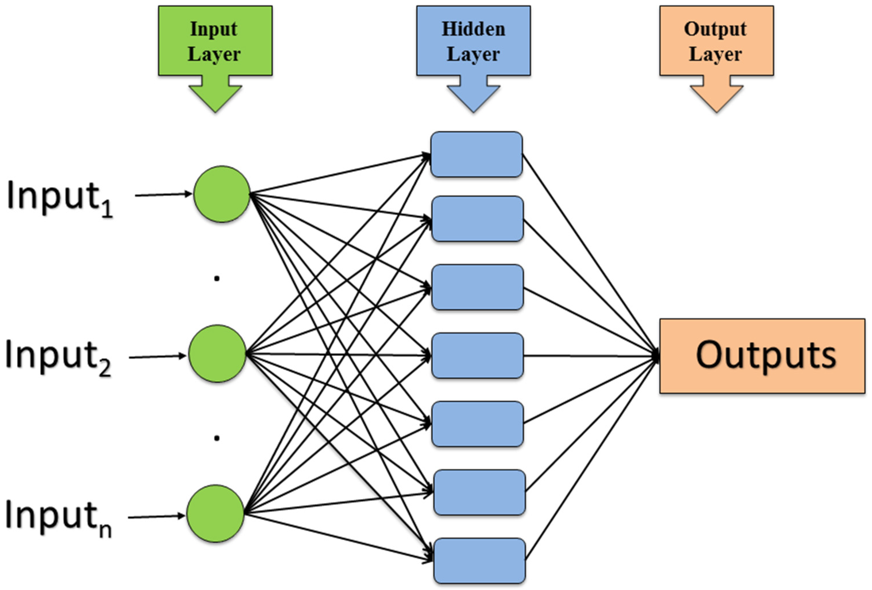
The ANN models were created using the multilayer perceptron (MLP) method, one of the models that researchers frequently adopt due to its strong learning capabilities. In terms of structure, MLP networks consist of three linked primary layers.

The prediction data is derived from the input layer, the hidden layer, and the output layer, which are the first, second, and third layers, respectively. In the developed ANN model, MLP structures with a single hidden layer are preferred. In the performance analysis of the designed ANN model, it has been shown that, in order to achieve ideal results, the number of hidden layers is sufficient and that it is not necessary to experiment on MLP models with multiple hidden layer structures. An MLP network model’s symbolic architecture is depicted in Figure 1. In each of the three distinct MLP network models, different input parameters were defined in order to estimate Nu values.

Table 1. Output and input values of three different ANN models.

	Inputs								Output
ANN Model-I	β	γ	Ec	Pr	ε	R	H		Nu
ANN Model-II	β	γ	Ec	Pr	ε	H	R1	R2	Nu
ANN Model-III	β	γ	Ec	Pr	ε	R	H1	H2	Nu

displays the input and output parameters of three distinct ANN models that were created. Moreover, R1 and R2 represent the thermal radiation parameter values 0 and 0.5, respectively. The same is the case for heat generation parameters H₁ and H₂. The performance of forecasts is impacted by the best data optimization during the building of ANN models. According to the grouping technique frequently employed in the literature, the data utilized in ANN models, each of which was produced with a different number of data sets, were segmented. A total of 15% of the data is set aside for validation, 15% for testing, and 70% is set aside for training.

Table 2. Information about the data set used in the development of three different ANN models.

	ANN Model-I	ANN Model-II	ANN Model-III
Training Data	48	84	84
Validation Data	11	18	18
Test Data	11	18	18
Total Data	70	120	120

provides details about the data set used to create three distinct ANN models. The optimization of the computational component known as the neuron in the hidden layer of MLP models is one of the challenges. Further, there is no model or guideline for calculating the number of neurons, which is the fundamental cause of this challenge. In the hidden layer, the number of neurons between 5 and 25 was tested. The MLP network model with 10 neurons in the hidden layer was chosen after the performances of other MLP networks with various numbers of hidden layer neurons were assessed. In determining the optimal number of neurons, parameters such as deviation rates, mean squared error (MSE) values, and coefficient of determination (Rm) values were taken into account. The Levenberg-Marquardt method, a popular training technique with excellent estimate performance, served as the ANN model’s training procedure [25]. In the hidden and output layers, respectively, there are Tan-Sig and Purelin functions acting as transfer functions. The transfer function mathematical expressions are shown below [26]:

$$f(x)=\frac{1}{1+e^{-x}},$$

(34)

Pureline(x) = x.

(35)

The MSE, Rm, and margin of deviation (MoD) metrics, which are often used in the literature, were chosen to examine the estimated performance of three ANN models. The following lists the mathematical formulas [27,28,29,30] used to calculate the performance parameters:

$$\mathrm{MSE}=\frac{1}{N}{\displaystyle \sum _{i=1}^N{(X_{\mathrm{num}(i)}-X_{\mathrm{ANN}(i)})}^2}.$$

(36)

$$Rm=\sqrt{1-\frac{{\displaystyle \sum _{i=1}^N{(X_{\mathrm{num}(i)}-X_{\mathrm{ANN}(i)})}^2}}{{\displaystyle \sum _{i=1}^N{(X_{\mathrm{num}(i)})}^2}}},$$

(37)

$$\mathrm{MoD}(\%)=\left[\frac{X_{\mathrm{num}}-X_{\mathrm{ANN}}}{X_{\mathrm{num}}}\right].$$

(38)

5. Comparative Analysis

The aim of this study is to predict the values of the heat transfer coefficient at a cylindrical surface when a non-Newtonian fluid passes over the surface. A total of three different flow regimes have been considered when constructing the corresponding ANN models. The ANN Model-I is developed by considering the Casson fluid flow over an inclined stretching cylinder along with the involved physical effects, namely an externally applied magnetic field, stagnation point flow, mixed convection, heat generation, viscous dissipation, thermal radiations, and variable thermal conductivity. In this model, we consider seven inputs and the Nusselt number as an output. The ANN Model-II is used to predict the Nusselt number values for two different thermal regimes, namely, the thermal regime with radiations and the thermal regime without radiations. The ANN Model-III offers the prediction of the Nusselt number for two different thermal regimes, namely, thermal regimes with and without heat generation. In using the shooting method, we obtained the numerical values of the Nusselt number for three different models (see

Table 3. Effect of Casson fluid parameter on Nusselt number.

$\mathit{\beta }$	${\mathit{\theta }}^{\prime }(0)$	$-[1+4/3\mathit{R}]{\mathit{\theta }}^{\prime }(0)$$,\mathit{R}=0.2$
0.2	−2.0221	2.5613
0.3	−1.9371	2.4536
0.4	−1.8933	2.3982
0.5	−1.8664	2.3641
0.6	−1.8481	2.3409
0.7	−1.8347	2.3239
0.8	−1.8246	2.3112
0.9	−1.8165	2.3009
01	−1.8100	2.2927
02	−1.7794	2.2539

,

Table 4. Impact of curvature parameter on Nusselt number.

$\mathit{\gamma }$	${\mathit{\theta }}^{\prime }(0)$	$-[1+4/3\mathit{R}]{\mathit{\theta }}^{\prime }(0)$$,\mathit{R}=0.2$
0.2	−0.9511	1.2047
0.3	−1.0468	1.3259
0.4	−1.1443	1.4494
0.5	−1.2441	1.5759
0.6	−1.3466	1.7057
0.7	−1.4515	1.8386
0.8	−1.5587	1.9744
0.9	−1.6681	2.1129
01	−1.7794	2.2539
02	−2.9651	3.7559

,

Table 5. Impact of Eckert number on Nusselt number.

Ec	${\mathit{\theta }}^{\prime }(0)$	$-[1+4/3\mathit{R}]{\mathit{\theta }}^{\prime }(0)$$,\mathit{R}=0.2$
0.2	−1.9015	2.4086
0.3	−2.0216	2.5608
0.4	−2.1397	2.7104
0.5	−2.2560	2.8577
0.6	−2.3705	3.0027
0.7	−2.4832	3.1455
0.8	−2.5943	3.2862
0.9	−2.7037	3.4247
01	−2.8116	3.5615
02	−3.2282	4.0892

,

Table 6. Impact of Prandtl number on Nusselt number.

Pr	${\mathit{\theta }}^{\prime }(0)$	$-[1+4/3\mathit{R}]{\mathit{\theta }}^{\prime }(0)$$,\mathit{R}=0.2$
0.2	−1.3536	1.7146
0.3	−1.3813	1.7496
0.4	−1.4084	1.7840
0.5	−1.4348	1.8175
0.6	−1.4607	1.8502
0.7	−1.4861	1.8824
0.8	−1.5109	1.9139
0.9	−1.5353	1.9448
01	−1.5593	1.9752
02	−1.7794	2.2540

,

Table 7. Impact of variable thermal conductivity on Nusselt number.

$\mathit{\epsilon }$	${\mathit{\theta }}^{\prime }(0)$	$-[1+4/3\mathit{R}]{\mathit{\theta }}^{\prime }(0)$$,\mathit{R}=0.2$
0.2	−3.0653	3.8828
0.3	−2.8466	3.6057
0.4	−2.6458	3.3514
0.5	−2.4588	3.1146
0.6	−2.2821	2.8907
0.7	−2.1121	2.6754
0.8	−1.9457	2.4646
0.9	−1.7794	2.2540
01	−1.6097	2.0390
02	−1.0271	1.3010

,

Table 8. Impact of radiation parameter on Nusselt number.

R	${\mathit{\theta }}^{\prime }(0)$	$-[1+4/3\mathit{R}]{\mathit{\theta }}^{\prime }(0)$
0.2	−1.7794	2.2539
0.3	−1.6752	2.3452
0.4	−1.5591	2.3906
0.5	−1.4325	2.3875
0.6	−1.2956	2.3320
0.7	−1.1483	2.2200
0.8	−0.9895	2.0449
0.9	−0.8162	1.7956
01	−0.6202	1.4471
02	−0.3629	1.3306

,

Table 9. Influence of heat generation parameter on Nusselt number.

H	${\mathit{\theta }}^{\prime }(0)$	$-[1+4/3\mathit{R}]{\mathit{\theta }}^{\prime }(0)$$,\mathit{R}=0.2$
0.2	−1.8322	2.3208
0.3	−1.8836	2.3859
0.4	−1.9338	2.4495
0.5	−1.9827	2.5115
0.6	−2.0305	2.5720
0.7	−2.0772	2.6312
0.8	−2.1230	2.6892
0.9	−2.1678	2.7459
01	−2.2118	2.8017
02	−2.2421	2.8401

,

Table 10. Impact of curvature parameter on Nusselt number for non-radiative and radiative flow fields.

$\mathit{\gamma }$	${\mathit{\theta }}^{\prime }(0)$		$-[1+4/3\mathit{R}]{\mathit{\theta }}^{\prime }(0)$
	R = 0	R = 0.5	R = 0	R = 0.5
0.2	−1.0677	−0.9493	1.0677	1.5822
0.3	−1.3171	−1.2061	1.3171	2.0105
0.4	−1.5766	−1.4739	1.5766	2.4569
0.5	−1.8443	−1.7494	1.8443	2.9163
0.6	−2.1182	−2.0306	2.1182	3.3851
0.7	−2.3970	−2.3160	2.3970	3.8607
0.8	−2.6796	−2.6045	2.6796	4.3417
0.9	−2.9653	−2.8953	2.9653	4.8264
1.0	−3.2535	−3.1881	3.2535	5.3146
2.0	−6.2049	−6.1651	6.2049	10.277

,

Table 11. Impact of Casson fluid parameter on Nusselt number for radiative and non-radiative flow fields.

$\mathit{\beta }$	${\mathit{\theta }}^{\prime }(0)$		$-[1+4/3\mathit{R}]{\mathit{\theta }}^{\prime }(0)$
	R = 0	R = 0.5	R = 0	R = 0.5
0.2	−3.3407	−3.2765	3.3407	5.4619
0.3	−3.3106	−3.2453	3.3106	5.4099
0.4	−3.2950	−3.2294	3.2950	5.3834
0.5	−3.2854	−3.2196	3.2854	5.3660
0.6	−3.2788	−3.2130	3.2788	5.3561
0.7	−3.2740	−3.2081	3.2740	5.3479
0.8	−3.2703	−3.2044	3.2703	5.3417
0.9	−3.2674	−3.2015	3.2674	5.3369
1.0	−3.2650	−3.1992	3.2650	5.3331
2.0	−3.2535	−3.1881	3.2535	5.3145

,

Table 12. Impact of Eckert number on Nusselt number for radiative and non-radiative flow fields.

E	${\mathit{\theta }}^{\prime }(0)$		$-[1+4/3\mathit{R}]{\mathit{\theta }}^{\prime }(0)$
	R = 0	R = 0.5	R = 0	R = 0.5
0.2	−3.2969	−3.2327	3.2969	5.3889
0.3	−3.3403	−3.2773	3.3403	5.4632
0.4	−3.3836	−3.3219	3.3836	5.5376
0.5	−3.4270	−3.3665	3.4270	5.6119
0.6	−3.4704	−3.4111	3.4704	5.6863
0.7	−3.5138	−3.4558	3.5138	5.7608
0.8	−3.5572	−3.5004	3.5572	5.8352
0.9	−3.6006	−3.5451	3.6006	5.9096
1.0	−3.6440	−3.5898	3.6440	5.9841
2.0	−4.0787	−4.0372	4.0787	6.7301

,

Table 13. Impact of Prandtl number on Nusselt number for non-radiative and radiative flow fields.

Pr	${\mathit{\theta }}^{\prime }(0)$		$-[1+4/3\mathit{R}]{\mathit{\theta }}^{\prime }(0)$
	R = 0	R = 0.5	R = 0	R = 0.5
0.2	−3.0932	−3.0717	3.0932	5.1205
0.3	−3.1265	−3.0956	3.1265	5.1604
0.4	−3.1592	−3.1191	3.1592	5.1995
0.5	−3.1912	−3.1424	3.1912	5.2384
0.6	−3.2227	−3.1654	3.2227	5.2767
0.7	−3.2535	−3.1881	3.2535	5.3145
0.8	−3.2839	−3.2105	3.2839	5.3519
0.9	−3.3137	−3.2326	3.3137	5.3887
1.0	−3.3431	−3.2546	3.3431	5.4254
2.0	−3.6149	−3.4617	3.6149	5.7706

,

Table 14. Impact of variable thermal conductivity on Nusselt numbers for radiative and non-radiative flow fields.

$\mathit{\epsilon }$	$\mathit{\theta }\prime (0)$		$-[1+4/3\mathit{R}]{\mathit{\theta }}^{\prime }(0)$
	R = 0	R = 0.5	R = 0	R = 0.5
0.2	−2.7937	−2.7799	2.7937	4.6341
0.3	−2.5894	−2.5450	2.5894	4.2425
0.4	−2.4047	−2.3224	2.4047	3.8714
0.5	−2.2353	−2.1076	2.2353	3.5134
0.6	−2.0777	−1.8965	2.0777	3.1614
0.7	−1.9285	−1.6847	1.9285	2.8084
0.8	−1.7848	−1.4671	1.7848	2.4456
0.9	−1.6436	−1.2373	1.6436	2.0625
1.0	−1.5720	−0.9852	1.5720	1.6423
2.0	−1.2825	−0.6896	1.2825	1.1496

,

Table 15. Impact of heat generation parameter on Nusselt number for radiative and non-radiative flow fields.

H	${\mathit{\theta }}^{\prime }(0)$		$-[1+4/3\mathit{R}]{\mathit{\theta }}^{\prime }(0)$
	R = 0	R = 0.5	R = 0	R = 0.5
0.2	−3.2670	−3.2020	3.2670	5.3377
0.3	−3.2805	−3.2159	3.2805	5.3609
0.4	−3.2938	−3.2298	3.2938	5.3841
0.5	−3.3072	−3.2436	3.3072	5.4071
0.6	−3.3204	−3.2573	3.3204	5.4299
0.7	−3.3337	−3.2709	3.3337	5.4526
0.8	−3.3468	−3.2845	3.3468	5.4753
0.9	−3.3599	−3.2981	3.3599	5.4979
1.0	−3.3730	−3.3116	3.3730	5.5204
2.0	−3.5007	−3.4432	3.5007	5.7398

,

Table 16. Impact of Casson fluid parameter on Nusselt number with and without heat generation.

$\mathit{\beta }$	${\mathit{\theta }}^{\prime }(0)$		$-[1+4/3\mathit{R}]{\mathit{\theta }}^{\prime }(0)$$,\mathit{R}=0.2$
	H = 0	H = 0.5	H = 0	H = 0.5
0.2	−3.2951	−3.3603	4.1739	4.2565
0.3	−3.2642	−3.3305	4.1347	4.2187
0.4	−3.2483	−3.3152	4.1146	4.1994
0.5	−3.2386	−3.3058	4.1023	4.1875
0.6	−3.2319	−3.2994	4.0938	4.1794
0.7	−3.2271	−3.2947	4.0877	4.1734
0.8	−3.2233	−3.2911	4.0829	4.1688
0.9	−3.2204	−3.2883	4.0793	4.1653
1.0	−3.2180	−3.2860	4.0762	4.1624
2.0	−3.2066	−3.2750	4.0618	4.1484

,

Table 17. Impact of curvature fluid parameter on Nusselt number with and without heat generation.

$\mathit{\gamma }$	${\mathit{\theta }}^{\prime }(0)$		$-[1+4/3\mathit{R}]{\mathit{\theta }}^{\prime }(0)$$,\mathit{R}=0.2$
	H = 0	H = 0.5	H = 0	H = 0.5
0.2	−0.9679	−1.1551	1.2256	1.4632
0.3	−1.2281	−1.3848	1.5556	1.7542
0.4	−1.4969	−1.6307	1.8961	2.0656
0.5	−1.7722	−1.8885	2.2448	2.3922
0.6	−2.0528	−2.1552	2.6003	2.7299
0.7	−2.3372	−2.4286	2.9605	3.0763
0.8	−2.6248	−2.7070	3.3248	3.4289
0.9	−2.9147	−2.9895	3.6921	3.7867
1.0	−3.2066	−3.2750	4.0618	4.1484
2.0	−6.1786	−6.2150	7.8264	7.8725

,

Table 18. Impact of Eckert number on Nusselt number with and without heat generation.

E	${\mathit{\theta }}^{\prime }(0)$		$-[1+4/3\mathit{R}]{\mathit{\theta }}^{\prime }(0)$$,\mathit{R}=0.2$
	H = 0	H = 0.5	H = 0	H = 0.5
0.2	−3.2508	−3.3182	4.1177	4.2032
0.3	−3.2950	−3.3613	4.1737	4.2577
0.4	−3.3392	−3.4045	4.2297	4.3125
0.5	−3.3835	−3.4477	4.2858	4.3672
0.6	−3.4277	−3.4909	4.3418	4.4219
0.7	−3.4720	−3.5341	4.3979	4.4766
0.8	−3.5162	−3.5773	4.4539	4.5313
0.9	−3.5605	−3.6206	4.4501	4.5862
1.0	−3.6048	−3.6638	4.5662	4.6409
2.0	−4.0481	−4.0967	5.1277	5.1893

,

Table 19. Impact of Prandtl number on Nusselt number with and without heat generation.

Pr	${\mathit{\theta }}^{\prime }(0)$		$-[1+4/3\mathit{R}]{\mathit{\theta }}^{\prime }(0)$$,\mathit{R}=0.2$
	H = 0	H = 0.5	H = 0	H = 0.5
0.2	−3.0786	−3.0996	3.8996	3.9263
0.3	−3.1050	−3.1360	3.9331	3.9724
0.4	−3.1310	−3.1717	3.9661	4.0176
0.5	−3.1566	−3.2068	3.9984	4.0621
0.6	−3.1818	−3.2412	4.0304	4.1058
0.7	−3.2066	−3.2750	4.0618	4.1484
0.8	−3.2311	−3.3083	4.0928	4.1906
0.9	−3.2553	−3.3410	4.1234	4.2321
1.0	−3.2791	−3.3732	4.1536	4.2728
2.0	−3.5026	−3.6719	4.4367	4.6512

,

Table 20. Impact of variable thermal conductivity on Nusselt number with and without heat generation.

$\mathit{\epsilon }$	${\mathit{\theta }}^{\prime }(0)$		$-[1+4/3\mathit{R}]{\mathit{\theta }}^{\prime }(0)$$,\mathit{R}=0.2$
	H = 0	H = 0.5	H = 0	H = 0.5
0.2	−2.7477	−2.8195	3.4805	3.5715
0.3	−2.5369	−2.6115	3.2135	3.3079
0.4	−2.3414	−2.4194	2.9658	3.0646
0.5	−2.1571	−2.2393	2.7324	2.8365
0.6	−1.9804	−2.0679	2.5086	2.6194
0.7	−1.8079	−1.9017	2.2901	2.4088
0.8	−1.6357	−1.7376	2.0719	2.2011
0.9	−1.4601	−1.5721	1.8495	1.9914
1.0	−1.2761	−1.4015	1.1664	1.7751
2.0	−0.8518	−1.0240	1.0789	1.2971

and

Table 21. Impact of thermal radiation parameter on Nusselt number with and without heat generation.

R	${\mathit{\theta }}^{\prime }(0)$		$-[1+4/3\mathit{R}]{\mathit{\theta }}^{\prime }(0)$
	H = 0	H = 0.5	H = 0	H = 0.5
0.2	−3.2066	−3.2750	4.0618	4.1484
0.3	−3.1941	−3.2629	4.4717	4.5681
0.4	−3.1833	−3.2526	4.8799	4.9862
0.5	−3.1740	−3.2436	5.2911	5.4071
0.6	−3.1658	−3.2356	5.6984	5.8241
0.7	−3.1585	−3.2286	6.1054	6.2408
0.8	−3.1519	−3.2222	6.5141	6.6593
0.9	−3.1459	−3.2164	6.9209	7.0761
1.0	−3.1404	−3.2111	7.3265	7.4915
2.0	−3.1012	−3.1731	11.372	11.635

). The impact of the Casson fluid parameter on the Nusselt number is presented in detail in Table 3. The numerical information for the Nusselt number for a positive iteration of the curvature parameter is presented in Table 4. Table 5 demonstrates the influence of Eckert number on Nusselt number, and as can be observed, Nusselt number exhibits a direct relationship with larger Eckert number values, i.e., Nusselt number grows in magnitude as Eckert number rises. Table 6 shows how Pr affects the Nusselt number.

The impact of the temperature-dependent variable viscosity parameter on the Nusselt number is inspected and given in Table 7, Table 8 and Table 9 shows the impact of heat generation and thermal radiation parameters on the Nusselt number. In detail, larger values of the thermal radiation parameter cause a decline in the Nusselt number while for large heat generation parameter, the Nusselt number shows inciting values.

Collectively, for Table 3, Table 4, Table 5, Table 6, Table 7, Table 8 and Table 9, it has been observed that the heat transfer normal to the cylindrical surface enhances for curvature parameter, Prandtl number and heat generation parameter while for Casson fluid, thermal conductivity, radiation parameters and Eckert number. In addition, it behaved in opposition to the impact of the curvature parameter on the Nusselt number is observed for two different values of the thermal radiation parameter that is R = 0 and R = 0.5 see Table 10. Further, for the two alternative values of the thermal radiation parameter, R = 0 and R = 0.5, are used to examine the impact of the Casson fluid parameter on the Nusselt number. Table 11 is provided in this context. It was observed that the Nusselt number dramatically decreases for positive Casson fluid parameter fluctuation. In both the presence and non-existence scenarios of thermal radiations, the influence of the Eckert number on the Nusselt number is seen see Table 12. Table 13 offers the impact of Pr on the Nusselt number for both radiative and non-radiative cases. Furthermore, in both cases, the Nusselt number is an increasing function of positive variation in Pr. Table 14 examines and provides information on the impact of a temperature-dependent variable viscosity parameter on the Nusselt number. The effects of heat generation on the Nusselt number are shown in Table 15. In this case, there were higher values of the heat production parameter reveal increasing levels for the Nusselt number. Collectively for Table 10, Table 11, Table 12, Table 13, Table 14 and Table 15, the magnitude of heat transfer normal to the cylindrical surface is higher for the case of presence of the thermal radiation effect. Table 16 offered the influence of the Casson fluid parameter on the Nusselt number is noticed for two different values namely H = 0 and H = 0.5. Further, H = 0 corresponds to the non-existence of the heat generation effect while H = 0.5 implied the existence of heat generation effect. In both cases, it is seen that the Nusselt number shows an inverse relation towards Casson fluid parameter.

The effects of the curvature fluid parameter on the Nusselt number are shown in Table 17 for two distinct values, H = 0 and H = 0.5. In addition, the Nusselt number is stronger in the case of the heat generating effect.

For two distinct scenarios, a thermal flow field with heat generation and a thermal flow field without heat generation, the impact of the Eckert number on Nusselt is explored see Table 18. The finding on the Nusselt number toward a positive fluctuation in the Prandtl number is presented in Table 19. As seen by past events, the Nusselt number rises sharply when provoked. Both the presence and absence of the heat generating effect are noted by such measurements. Additionally, it is noted that the Nusselt number’s magnitude is greater for thermal flow fields with heat generating effects. For both thermal fields, namely thermal flow regimes with and without heat generating effect, the effect of changing thermal conductivity parameter on Nusselt number is perceived. To that end, Table 20 is provided. When there is a thermal flow regime and a heat generating impact, the Nusselt number is larger. The observation of the Nusselt number toward a positive fluctuation in the thermal radiation parameter is shown in Table 21. Both the presence and absence of the heat generating effect are observed and recorded. Furthermore, it is shown that the Nusselt number magnitude is a little bit bigger when the influence of heat generation is present. While the heat transfer normal to the cylindrical surface exhibits encouraging values for the Prandtl number, curvature parameter, Eckert number, and thermal radiations, the Casson fluid parameter and the temperature dependent variable viscosity parameter exhibit the opposite behavior. Furthermore, we have shown that the magnitude of the Nusselt number is larger when thermal radiations are present. The estimated MSE and R values for every ANN model for the training, validation, and testing phases are displayed in

Table 22. Performance results for ANN models.

	MSE			Rm
	Training	Validation	Test	Training	Validation	Test
ANN Model-I	9.88 × 10−3	3.87 × 10−2	3.24 × 10−3	0.98624	0.96049	0.96282
ANN Model-II	3.34 × 10−4	1.31 × 10−3	2.11 × 10−3	0.99993	0.99972	0.99201
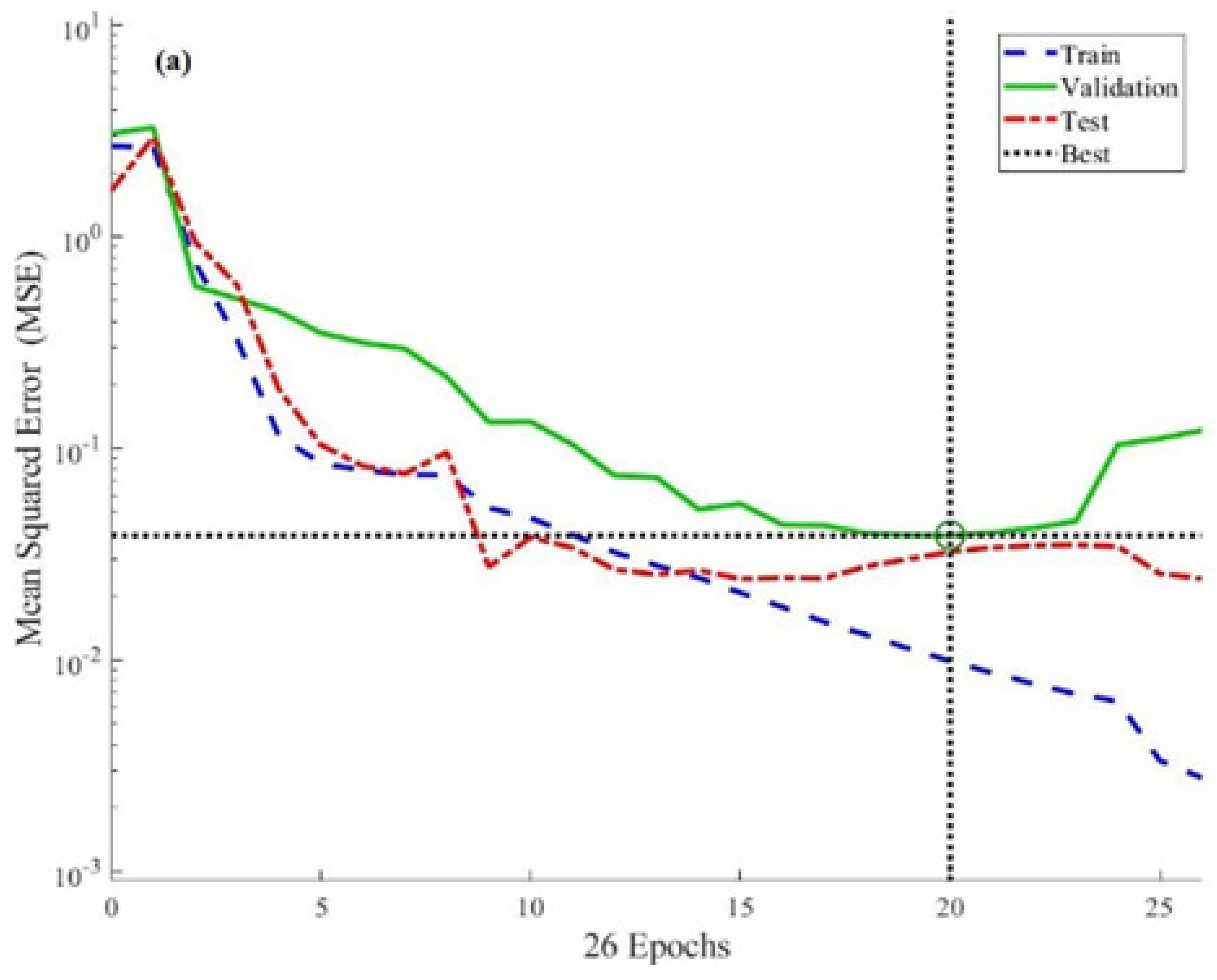
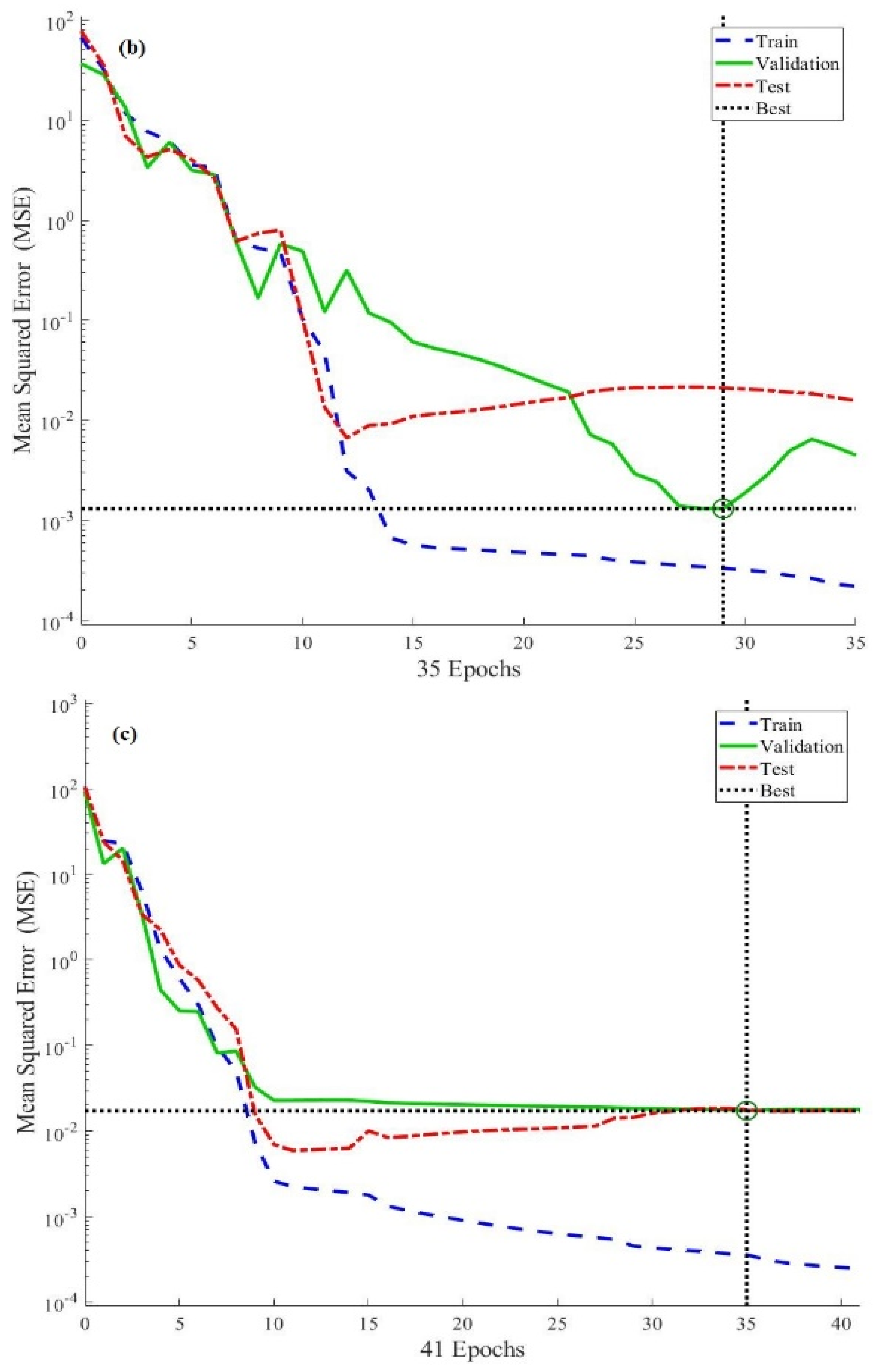
ANN Model-III	3.59 × 10−4	1.73 × 10−2	1.78 × 10−3	0.99993	0.99576	0.99861

. The fact that the R-value is extremely near to 1 and the MSE value is low demonstrates the great accuracy with which the generated ANN models can predict the Nusselt number. For each flow regime, we have constructed ANN models and the procedure is supported graphically. In particular, the validation that the training period, which began with the entrance of the data into the system, is ideally finished, is the first stage in the construction of ANN models. In Figure 2a, the ANN Model-I training performance graphs are created while the training performance of the ANN Model-II is developed in Figure 2b. Figure 2c provides the training performance of the ANN model-III. In networks with MLP design, the training cycle is repeated until there is the minimal error between the target data and the prediction data acquired in the output layer. With each epoch, the MSE values, which are large at the start of the training phase, go smaller. The findings shown in Figure 2a–c demonstrate that the constructed ANN models for predicting the Nusselt number have successfully completed their training phases. The examination of error histograms are a further step in evaluating the training performance of ANN models to forecast the Nusselt number. The error histograms for ANN models I, II, and III are shown in Figure 3a–c, respectively. The error histograms display the discrepancies between the goal values attained during the training phase and the anticipated values. The errors obtained for each ANN model are shown to cluster around the zero-error line, according to our observations. The numerical quantities of the inaccuracies are also relatively modest, which should be emphasized.

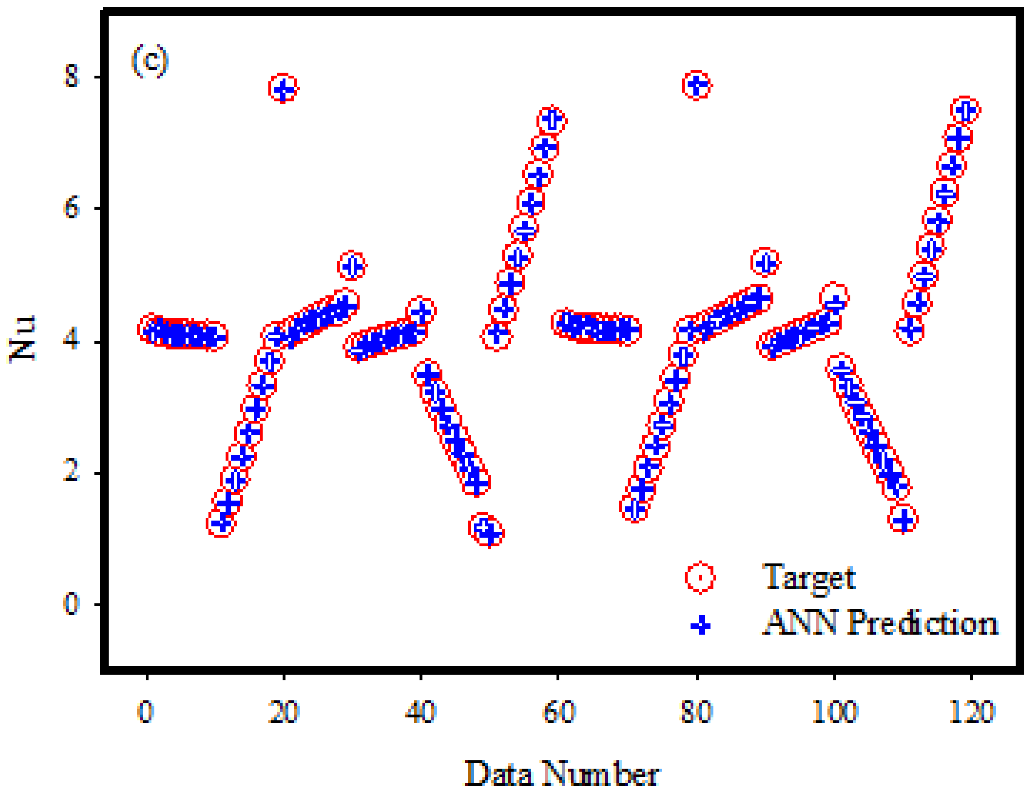
The findings from the error histograms demonstrate that a little error is carried out throughout the training stages of the three distinct ANN models that were created to predict the Nusselt number. Figure 4a–c depict the output values and target values obtained from the ANN models, designated as Model-I, Model-II and Model-III, each of which was developed using data sets with different data numbers.

In the analysis of each data point, it is evident that the goal data and the data from the ANN models (I,II,III) are in perfect harmony. The generated ANN models can estimate the Nusselt number with great accuracy, as demonstrated by the perfect match of the outputs derived from the ANN estimations with the target data. Figure 5a. Figure 5b,c display the MoD values that represent the proportional deviation between the target data and the outputs from three distinct ANN models created for predicting Nusselt number parameters based on various input parameters.

It can be noted that the data points are typically close to the zero-deviation line and have low values when the data points reflecting the MoD values for ANN Models I, II, and III are inspected. The average MoD values calculated for Model-I, Model-II and Model-III are obtained as 0.01%, 0.01% and 0.06%, respectively. The low MoD values show that there is relatively little variation between the goal values and the projected values derived from the created ANN models. 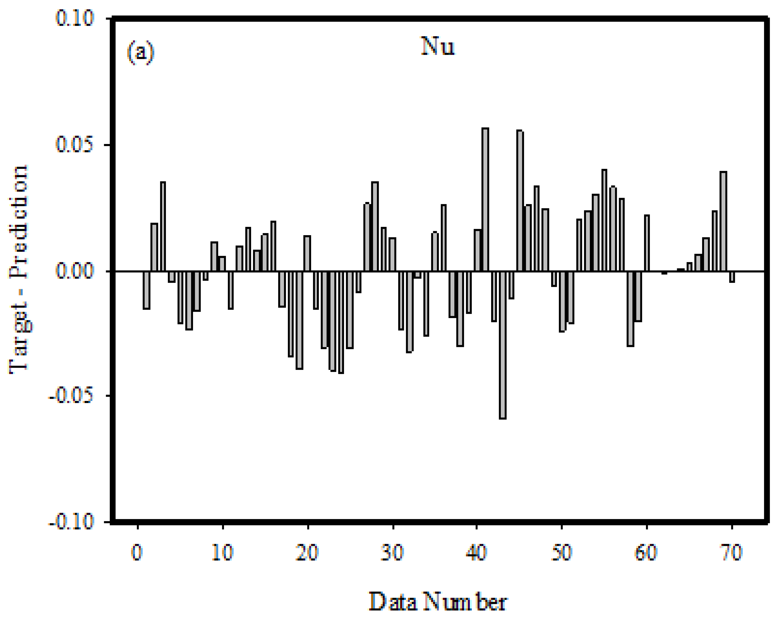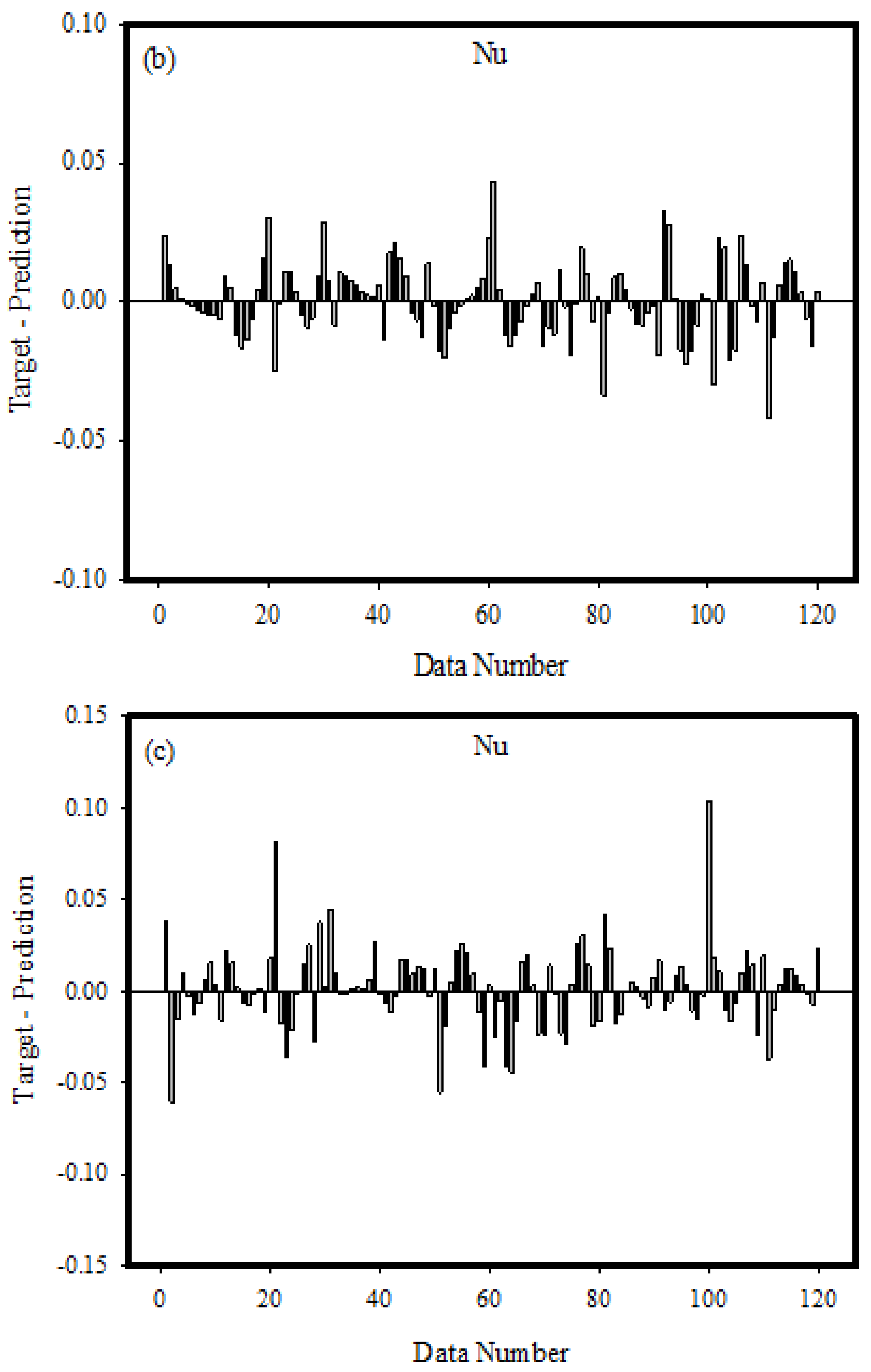In addition to the MoD values, the disparities between the target values and the ANN models’ outputs are examined for each output value in Figure 6a–c. Each ANN model has, in general, relatively modest differences when the different values obtained for each data point utilized in ANN model training are taken into account. The findings from the analysis of MoD and difference values show that both ANN models (I,II,III) developed can predict Nusselt number with very low errors. 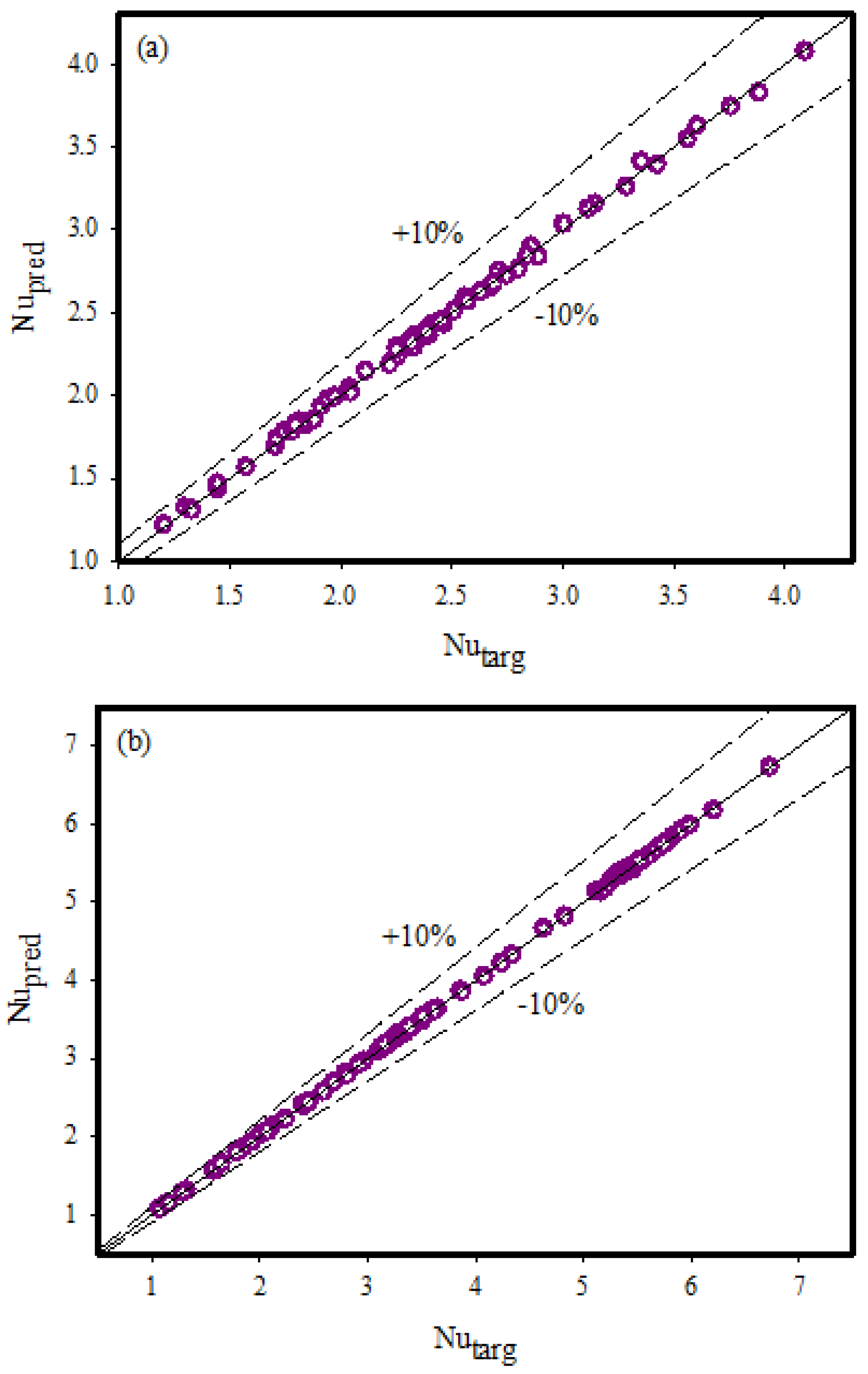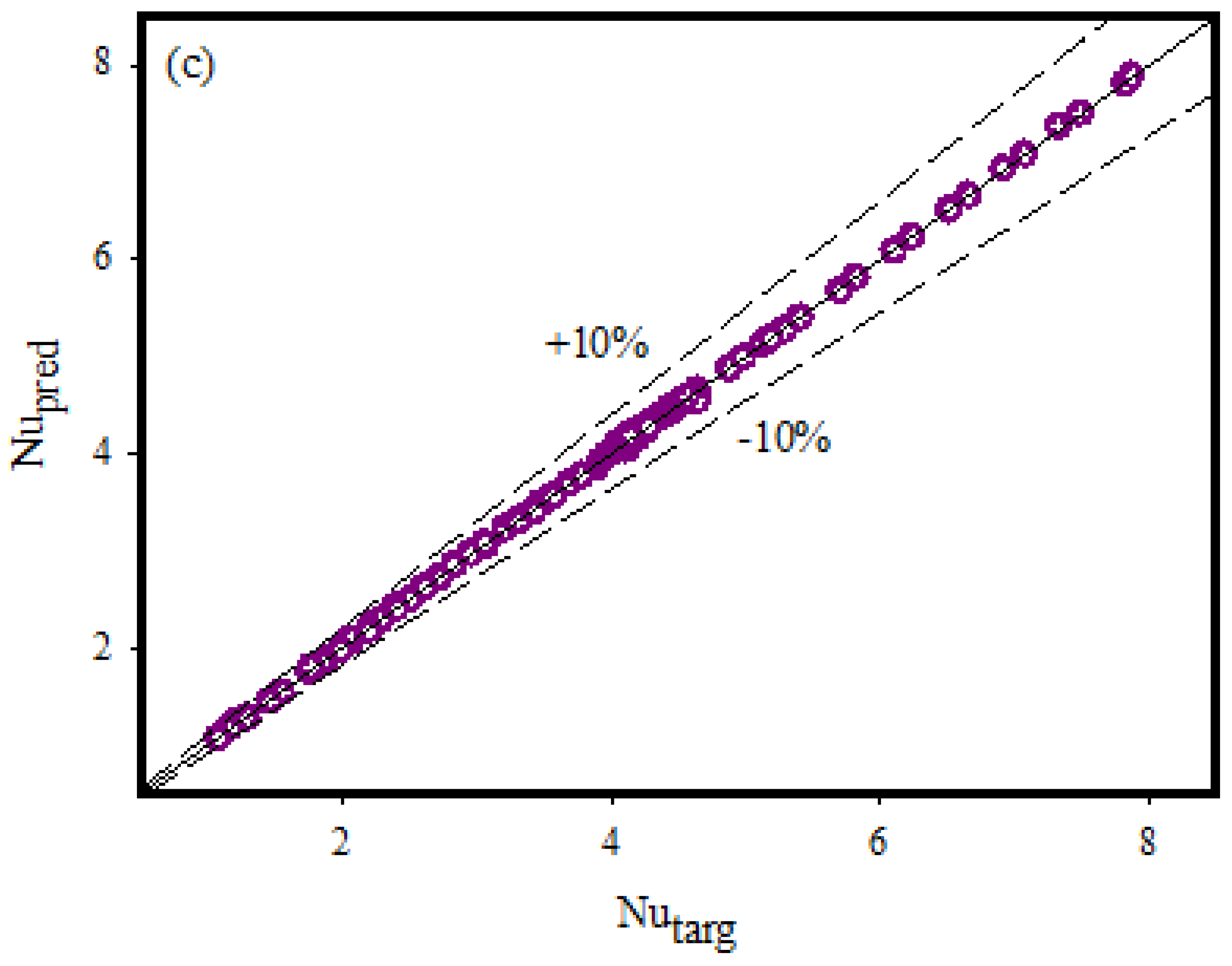Figure 7a–c titled Model-I, Model-II, and Model-III, respectively, illustrate the targeted and ANN outputs for each of the three ANN models. The data for each ANN model is often found on the zero-error line when the positions of the data points are taken into account. Additionally, it should be mentioned that the data points fall within a 10% error range. It is noticed that in the absence of magnetic field and heat generation effects, our problems reduced to Hayat et al. [31]. Additionally, for comparison, the Nusselt number is taken into consideration. In this direction,

Table 23. Comparison of Nusselt number with Hayat et al. [31].

$\mathit{\epsilon }$	$\mathit{\beta }$	$\mathit{\gamma }$	Hayat et al. [31]	Present Study
0.0	1.0	0.2	0.5276	0.5054
0.0	1.4	0.2	0.5316	0.5203
0.0	1.8	0.2	0.5336	0.5124
0.0	2.0	0.0	0.5442	0.5220
0.0	2.0	0.12	0.5336	0.5213
0.0	2.0	0.19	0.5279	0.5016
0.0	2.0	0.19	0.5739	0.5216
0.2	2.0	0.19	0.5308	0.5124
0.3	2.0	0.19	0.5123	0.5061

is offered in this regard. A perfect match that yields the surety of the present study was found.

6. Conclusions

An artificial neural networking models are developed to predict the heat transfer normal to the cylindrical surface for the incompressible flow of a two-dimensional mixed convection Casson fluid. The magnetic field is generated outside. In addition, it is presumed that the surface temperature is stronger than the surrounding fluid temperature. Further, the energy equation is carried with viscous dissipation, variable thermal conductivity, heat production, and thermal radiations. The following are the main results:

• Nusselt number shows inciting nature towards the Eckert number, curvature parameter, Prandtl number, and heat generation parameter
• Nusselt number admits declining trends toward the Casson fluid parameter, temperature-dependent thermal conductivity, and radiation parameters.
• The MSE and R values for Models I, II, and III are low and hence the developed ANN models can predict the Nusselt number with good accuracy.
• MoD outcomes show that there is not much of a discrepancy between the predicted and targeted values of the Nusselt number produced by the ANN models I, II, and III.
• The data points are often positioned on the zero-error line and fall within the 10% error region for ANN models I, II, and III to forecast the Nusselt number.
• Obtaining future data by using ANN models can provide many advantages in terms of both time and finance. In particular, obtaining specific parameters that can be obtained as a result of experimental studies by using ANN models can be considered an important advantage in both industrial applications and scientific studies.

References

1. Casson, N. A flow equation for pigment-oil suspensions of the printing ink type. In Rheology of Disperse Systems; Mill, C.C., Ed.; Pergamon Press: Oxford, UK, 1959; pp. 84–104. [Google Scholar]
2. Mustafa, M.; Hayat, T.; Ioan, P.; Hendi, A. Stagnation-point flow and heat transfer of a Casson fluid towards a stretching sheet. Z. Für Nat. A 2012, 67, 70–76. [Google Scholar] [CrossRef]
3. Mukhopadhyay, S. Casson fluid flow and heat transfer over a nonlinearly stretching surface. Chin. Phys. B 2013, 22, 074701. [Google Scholar] [CrossRef]
4. Mukhopadhyay, S.; Mondal, I.C.; Chamkha, A.J. Casson fluid flow and heat transfer past a symmetric wedge. Heat Transf. Asian Res. 2013, 42, 665–675. [Google Scholar] [CrossRef]
5. Pramanik, S. Casson fluid flow and heat transfer past an exponentially porous stretching surface in presence of thermal radiation. Ain Shams Eng. J. 2014, 5, 205–212. [Google Scholar] [CrossRef] [Green Version]
6. Mahdy, A. Heat transfer and flow of a Casson fluid due to a stretching cylinder with the Soret and Dufour effects. J. Eng. Phys. Thermophys. 2015, 88, 928–936. [Google Scholar] [CrossRef]
7. Abbas, Z.; Sheikh, M.; Motsa, S.S. Numerical solution of binary chemical reaction on stagnation point flow of Casson fluid over a stretching/shrinking sheet with thermal radiation. Energy 2016, 95, 12–20. [Google Scholar] [CrossRef]
8. Raju, C.S.K.; Hoque, M.M.; Sivasankar, T. Radiative flow of Casson fluid over a moving wedge filled with gyrotactic microorganisms. Adv. Powder Technol. 2017, 28, 575–583. [Google Scholar] [CrossRef]
9. Reddy, G.J.; Kethireddy, B.; Umavathi, J.C.; Sheremet, M.A. Heat flow visualization for unsteady Casson fluid past a vertical slender hollow cylinder. Therm. Sci. Eng. Prog. 2018, 5, 172–181. [Google Scholar] [CrossRef]
10. Sulochana, C.; Ashwinkumar, G.P.; Sandeep, N. Effect of frictional heating on mixed convection flow of chemically reacting radiative Casson nanofluid over an inclined porous plate. Alex. Eng. J. 2018, 57, 2573–2584. [Google Scholar] [CrossRef]
11. Ali, A.; Umar, M.; Bukhari, Z.; Abbas, Z. Pulsating flow of a micropolar-Casson fluid through a constricted channel influenced by a magnetic field and Darcian porous medium: A numerical study. Results Phys. 2020, 19, 103544. [Google Scholar] [CrossRef]
12. Gbadeyan, J.A.; Titiloye, E.O.; Adeosun, A.T. Effect of variable thermal conductivity and viscosity on Casson nanofluid flow with convective heating and velocity slip. Heliyon 2020, 6, e03076. [Google Scholar] [CrossRef] [Green Version]
13. Alizadeh, R.; Gomari, S.R.; Alizadeh, A.; Karimi, N.; Li, L.K. Combined heat and mass transfer and thermodynamic irreversibilities in the stagnation-point flow of Casson rheological fluid over a cylinder with catalytic reactions and inside a porous medium under local thermal nonequilibrium. Comput. Math. Appl. 2021, 81, 786–810. [Google Scholar] [CrossRef]
14. Jamshed, W.; Goodarzi, M.; Prakash, M.; Nisar, K.S.; Zakarya, M.; Abdel-Aty, A.H. Evaluating the unsteady Casson nanofluid over a stretching sheet with solar thermal radiation: An optimal case study. Case Stud. Therm. Eng. 2021, 26, 101160. [Google Scholar] [CrossRef]
15. Khan, M.R.; Al-Johani, A.S.; Elsiddieg, A.M.A.; Saeed, T.; Mousa, A.A.A. The computational study of heat transfer and friction drag in an unsteady MHD radiated Casson fluid flow across a stretching/shrinking surface. Int. Commun. Heat Mass Transf. 2022, 130, 105832. [Google Scholar] [CrossRef]
16. Ali, G.; Ali, F.; Khan, A.; Ganie, A.H.; Khan, I. A generalized magnetohydrodynamic two-phase free convection flow of dusty Casson fluid between parallel plates. Case Stud. Therm. Eng. 2022, 29, 101657. [Google Scholar] [CrossRef]
17. Ahmad, S.; Haq, S.U.; Ali, F.; Khan, I.; Nisar, K.S. Time fractional analysis of channel flow of couple stress Casson fluid using Fick’s and Fourier’s Laws. Sci. Rep. 2022, 12, 2956. [Google Scholar] [CrossRef]
18. Shahzad, H.; Wang, X.; Ghaffari, A.; Iqbal, K.; Hafeez, M.B.; Krawczuk, M.; Wojnicz, W. Fluid structure interaction study of non-Newtonian Casson fluid in a bifurcated channel having stenosis with elastic walls. Sci. Rep. 2011, 12, 12219. [Google Scholar] [CrossRef]
19. Xiao, B.; Wang, W.; Zhang, X.; Long, G.; Fan, J.; Chen, H.; Deng, L. A novel fractal solution for permeability and Kozeny-Carman constant of fibrous porous media made up of solid particles and porous fibers. Powder Technol. 2019, 349, 92–98. [Google Scholar] [CrossRef]
20. Liang, M.; Fu, C.; Xiao, B.; Luo, L.; Wang, Z. A fractal study for the effective electrolyte diffusion through charged porous media. Int. J. Heat Mass Transf. 2019, 137, 365–371. [Google Scholar] [CrossRef]
21. Hosseini, N.; Khoei, A.R. Modeling Fluid Flow in Fractured Porous Media with the Interfacial Conditions Between Porous Medium and Fracture. Transp. Porous Media 2021, 139, 109–129. [Google Scholar] [CrossRef]
22. Xiao, B.; Fang, J.; Long, G.; Tao, Y.; Huang, Z. Analysis of Thermal Conductivity of Damaged Tree-Like Bifurcation Network with Fractal Roughened Surfaces. Fractals 2022, 30, 2250104. [Google Scholar] [CrossRef]
23. Rehman, K.U.; Malik, M.Y.; Zehra, I.; Alqarni, M.S. Group theoretical analysis for MHD flow fields: A numerical result. J. Braz. Soc. Mech. Sci. Eng. 2019, 41, 156. [Google Scholar] [CrossRef]
24. Khan, I.; Rehman, K.U.; Malik, M.Y.; Aly, S. On magnetized non-Newtonian rotatory fluid flow field. Adv. Mech. Eng. 2019, 11, 1687814019878914. [Google Scholar] [CrossRef]
25. Çolak, A.B. An experimental study on the comparative analysis of the effect of the number of data on the error rates of artificial neural networks. Int. J. Energy Res. 2021, 45, 478–500. [Google Scholar] [CrossRef]
26. Öcal, S.; Gökçek, M.; Çolak, A.B.; Korkanç, M. A comprehensive and comparative experimental analysis on thermal conductivity of TiO2-CaCO3/Water hybrid nanofluid: Proposing new correlation and artificial neural network optimization. Heat Transf. Res. 2021, 52, 55–79. [Google Scholar] [CrossRef]
27. Çolak, A.; Güzel, T.; Yıldız, O.; Özer, M. An experimental study on determination of the shottky diode current-voltage characteristic depending on temperature with artificial neural network. Phys. B Condens. Matter 2021, 608, 412852. [Google Scholar] [CrossRef]
28. Rehman, K.U.; Shatanawi, W.; Çolak, A.B. Thermal analysis of flowing stream in partially heated double forward-facing step by using artificial neural network. Case Stud. Therm. Eng. 2022, 37, 102221. [Google Scholar] [CrossRef]
29. Çolak, A.B.; Karakoyun, Y.; Acikgoz, O.; Yumurtaci, Z.; Dalkilic, A.S. A numerical study aimed at finding optimal artificial neural network model covering experimentally obtained heat transfer characteristics of hydronic underfloor radiant heating systems running various nanofluids. Heat Transf. Res. 2022, 53, 51–71. [Google Scholar] [CrossRef]
30. Cao, Y.; Kamrani, E.; Mirzaei, S.; Khandakar, A.; Vaferi, B. Electrical efficiency of the photovoltaic/thermal collectors cooled by nanofluids: Machine learning simulation and optimization by evolutionary algorithm. Energy Rep. 2022, 8, 24–36. [Google Scholar] [CrossRef]
31. Hayat, T.; Asad, S.; Alsaedi, A. Flow of variable thermal conductivity fluid due to inclined stretching cylinder with viscous dissipation and thermal radiation. Appl. Math. Mech. 2014, 35, 717–728. [Google Scholar] [CrossRef]
Figure 1. The symbolic architecture of an MLP network model.
Mathematics 11 00342 g001
Figure 2. (a) Training performance of ANN model-I. (b) Training performance of ANN model-II. (c) Training performance of ANN model-III.
Mathematics 11 00342 g002aMathematics 11 00342 g002b
Figure 3. (a) Error histograms for of ANN model-I. (b) Error histograms for of ANN model-II. (c) Error histograms for of ANN model-III.
Mathematics 11 00342 g003aMathematics 11 00342 g003b
Figure 4. (a) The output values and target values obtained from ANN model-I. (b) The output values and target values obtained from ANN model-II. (c) The output values and target values obtained from ANN model-III.
Mathematics 11 00342 g004aMathematics 11 00342 g004b
Figure 5. (a) The MoD values for ANN model-I. (b) The MoD values for ANN model-II. (c) The MoD values for ANN model-III.
Mathematics 11 00342 g005aMathematics 11 00342 g005b
Figure 6. (a) The variations between the targeted values and the outputs of the ANN model-I. (b) The variations between the goal values and the outputs of the ANN model-II. (c) The variations between the goal values and the outputs of the ANN model-III.
Mathematics 11 00342 g006aMathematics 11 00342 g006b
Figure 7. (a) The target and prediction values for ANN model-I. (b) The target and prediction values for ANN model-II. (c) The target and prediction values for ANN model-III.
Mathematics 11 00342 g007aMathematics 11 00342 g007b