Constructing Traceability Links between Software Requirements and Source Code Based on Neural Networks

Abstract

Software requirement changes, code changes, software reuse, and testing are important activities in software engineering that involve the traceability links between software requirements and code. Software requirement documents, design documents, code documents, and test case documents are the intermediate products of software development. The lack of interrelationship between these documents can make it extremely difficult to change and maintain the software. Frequent requirements and code changes are inevitable in software development. Software reuse, change impact analysis, and testing also require the relationship between software requirements and code. Using these traceability links can improve the efficiency and quality of related software activities. Existing methods for constructing these links need to be better automated and accurate. To address these problems, we propose to embed software requirements and source code into feature vectors containing their semantic information based on four neural networks (NBOW, RNN, CNN, and self-attention). Accurate traceability links from requirements to code are established by comparing the similarity between these vectors. We develop a prototype tool RCT based on this method. These four networks’ performances in constructing links are explored on 18 open-source projects. The experimental results show that the self-attention network performs best, with an average $Recall@50$ value of 0.687 on the 18 projects, which is higher than the other three neural network models and much higher than previous approaches using information retrieval and machine learning.

1. Introduction

Approximately 40% of the problems in software development are related to software requirements engineering [1]. Software engineering is about solving real-life problems through software technology, whereas requirements engineering defines the issues that need to be solved. Its goal is to use a systematic approach and engineering management tools to efficiently develop software requirements specifications and specific performance parameters that accurately express user needs.

In the current era of rapidly changing software requirements, it is unrealistic to ask the customer to set forward all requirements at once and never change them again, which means that changes to software requirements are inevitable. Therefore, the difficulty of software requirements management is caused by the requirements’ volatility. It has been observed that requirements change at different stages of the software development lifecycle and that such changes play a critical role in the success of a project. Usually, requirements change is caused by differences in developer understanding, changes in user business requirements, and normal system upgrades. Changes to source code and related software engineering products inevitably accompany changes in requirements. Constructing links between software requirements and software design documents, source code, and test cases are essential for software requirement relationships. For example, to test the implementation code of a modified requirement, the test cases must be adjusted accordingly. Software test managers need to understand the possible impact of requirements changes on product quality and requirements testing. Therefore, analyzing the relationships between software engineering artifacts produced during different software development lifecycles can improve the accuracy of change impact analysis.

Requirements traceability is defined as the ability to describe and track the lifecycle of requirements, including the ability to trace backwards and forwards through periods of continuous refinement and iteration. The construction of requirements traceability relationships can support various software engineering activities, including change impact analysis, regression test selection, cost prediction, and compliance validation [2]. The need to establish and maintain traceability links between requirements, design, code, faults, and test cases to demonstrate that the software system is safe to use is specified in regulatory standards for high-reliability systems (e.g., Federal Aviation Authority (FAA) standard DO178b/c) [3]. However, creating traceability relationships is more difficult and is prone to errors or omissions. In practice, manually creating traceability links or capturing them as a byproduct of the development process is often incomplete and inaccurate [4], even in some critical security systems [5]. In particular, software source code has a higher level of structured information and inherent complexity than other modules in a software system, containing more semantic and functional features that represent the software system. This makes it possible to develop requirements-to-code tracing tools that will support the field of software engineering and are essential for improving the efficiency and quality of software development.

Existing automated methods for establishing requirements and code traceability links can be classified as follows: information retrieval, program analysis, machine learning, etc. Information retrieval (IR) is the most commonly used method for establishing links [6,7,8,9,10]. The core idea of using IR to establish traceability is to extract comments, tokens, and key phrases from source code and requirement documents, then vectorize them using LSA, VSM, TF-IDF, and topic modeling. Finally, the similarity between them is used to determine whether links exist. These methods all split software requirements or source code into combinations of words or terms without understanding the conceptual connections between them [11], and the embedded semantic information in these artifacts is lost. This is caused by the lack of ability of these techniques to reason about the semantic relatedness between software artifacts. These approaches ignore conceptually similar tokens. For example, “audio” may be represented as “audio” in the requirements but is often expressed as “stream” in the code. This is a vocabulary mismatch problem. As a result, conventional information retrieval methods may not be able to establish links between files that contain overlapping terms. Most current technologies cannot reason about semantic associations between artifacts. Thus, traceability links in software can only be constructed when the words used overlap.

Deep learning techniques have now been successfully applied to solve many natural language processing (NLP) tasks, including text parsing [12], sentiment analysis [13] and machine translation [14]. Deep learning techniques divide the problem into multiple layers of nonlinear processing nodes. They use supervised or unsupervised learning techniques to automatically learn a linguistic or textual representation, which is then used to perform complex NLP tasks. This paper aims to use deep learning to provide scalable, portable, and fully automated solutions for constructing links between software requirements and code to bridge the semantic gap that currently prevents traceability link creation algorithms.

Aiming at the problems existing in the automatic establishment of requirement-code traceability link and the advantages of deep learning in processing natural language, this paper proposes a neural-network-based software requirement and source code tracing method (RCT). The method can automatically construct horizontal tracing links between software requirements and source code. Hindle et al. [15] showed that programming languages are comparable and predictive, similar to natural languages. The semantic gap that prevents the construction of tracing links can be bridged using deep learning. Word embeddings can learn the semantics of each word and represent it as a continuous high-dimensional word vector so that similar words are adjacent in the vector space. Neural networks can use these word vectors to learn the semantics of requirements and sentences or code segments in source code. For example, recurrent neural networks (RNNs) are suitable for processing sequential data such as text and audio. The core idea of RCT is to convert requirements and source code documents into same-dimensional feature vectors and determine whether they are linked by comparing the similarity between them. First, requirement-code link data are collected from open-source software repositories (e.g., GitHub) and preprocessed. This includes removing useless information, such as constructors and duplicate functions, from the code files, and parsing function names or tokens within functions named with camel or underscore. Secondly, we use four neural network models to embed the preprocessed software requirements and words or sentences from the source code into spatial vectors and then fuse these vectors using pooling functions or fully connected layers. Since these embedded spatial vectors contain semantic information about each word and implicit semantic associations between the requirements and code segments, the problem of “vocabulary mismatch” and semantic gaps is solved compared to information retrieval or machine learning methods. Finally, the links between software requirements and source code are constructed by calculating the spatial distance or cosine similarity between them and ranking them according to their similarity. The optimal neural network model is selected based on the experimental results. In addition, the dataset used for training and validating includes many different open-source projects, reducing the impact of differences in developers’ coding styles and habits and improving the generalization of the tracing model to real-world scenarios. We made our codes publicly available at: https://drive.google.com/drive/folders/1MadnriCIU0ShohG_csfKaTzJqm6FvQsy?usp=share_link (accessed on 30 December 2022).

To sum up, the main contributions of this paper are as follows:

1.

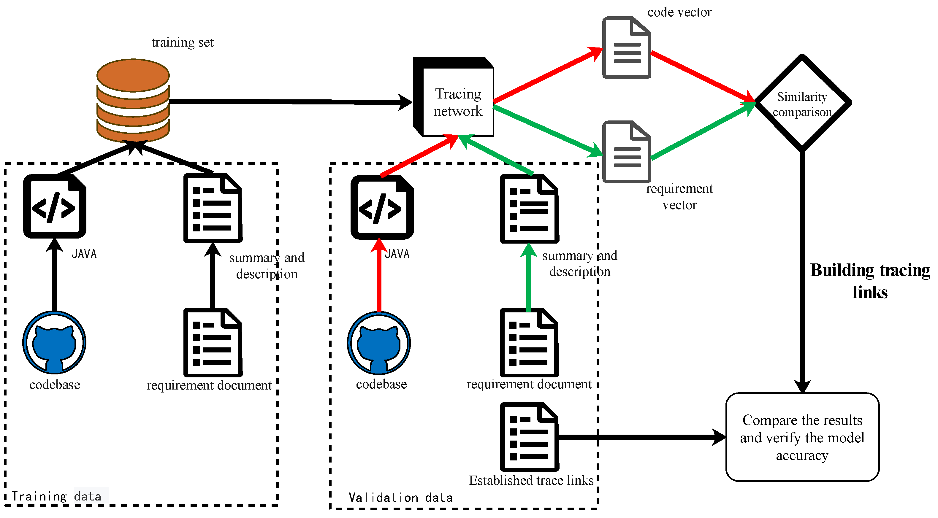
We propose a generic and automated technique for mapping software requirements to source code.

2.

We use a combination of neural network techniques to extract semantic information from software artifacts.

3.

We develop DCT, a tool for constructing traceability links between software requirements and source code.

4.

We demonstrate that self-attention is better at constructing traceability networks than other neural network models.

5.

We demonstrate that neural network technology can surpass or even substitute information retrieval techniques in traceability tasks.

The remainder of the paper is structured as follows. We first introduce techniques and works related to the tracing network in Section 2. The overview of our approach is described in Section 3. Section 4 and Section 5 describe the subject programs and metrics, our experiment process, the results achieved, and the discussion. Finally, the conclusion is summarized in Section 6.

2. Related Works

Change is an intrinsic feature of the software engineering discipline compared to other engineering disciplines. Due to the ever-changing scenarios and environments in which software is used, it is difficult to specify all its requirements simultaneously. Factors such as customer requirements, market changes, and peer competition can all lead to changes in requirements. Nurmuliani [16] defines requirements fluctuation as “the tendency for requirements to change over time in response to constant changes in the customer, the organization, and the work environment”. The main factors contributing to the failure of software projects are given in the Standish Group report [17]. As seen from the data in

Table 1. Factors that cause software projects to fail.

	Reasons for Failure	Proportions (%)
1	Incomplete requirements	13.1
2	Lack of user engagement	12.4
3	Lack of resources	10.6
4	Unrealistic expectations	9.9
5	Lack of administrative support	9.3
6	Changes in the requirements specification	8.7
7	Lack of project plan	8.1
8	The user no longer needs	7.5
9	Lack of IT management	6.2
10	Technical error	4.3
11	other	9.9

, the most significant causes of failure in these projects are related to requirements, particularly requirements change and the addition of new requirements. Their study also shows that requirements changes can increase project costs by a factor of three and project time by a factor of two. Furthermore, Huang et al.’s study also indicates that 40–90% of the total software development cost is spent on dealing with issues related to requirement changes [18]. Managing these change requirements has proven to be a significant challenge in requirements engineering [19,20]. Unmanaged or poorly managed changes to requirements can spell disaster for system development. These negative consequences can lead to software cost and schedule overruns, unstable requirements, endless testing, and, ultimately, project failure and business loss [16,21,22]. Therefore, change management can be both rewarding and challenging and is one of the essential factors in the success of a software project.

Requirements traceability is the core of software requirements management. A key component of requirements traceability is constructing links between software requirements and software design documents, source code, and test cases. However, much of the existing research is requirements-focused, ignoring the tracing of requirements to other software artifacts [23,24,25,26,27,28,29,30,31,32,33]. Changes to requirements can affect almost all software artifacts along the relationship between entities in the software development lifecycle. Analyzing the relationships between software engineering artifacts can improve the accuracy of change impact analysis. In particular, software source code has a higher level of structured information and inherent complexity than other modules in a software system. It can contain more semantic and functional features that represent the software system.

Manually creating links between software requirements and source code can be performed, but it is costly, especially for large software systems. The program analysis approach [9,34] is analyzed and implemented by automating the selection of the two main information dimensions in requirements and code, i.e., the dependencies between textual information (requirements text and source code files) and code elements (e.g., function call relationships and data dependencies). Information retrieval (IR) is still the most commonly used method for establishing traceability links [6,7,8,9,10]. Vale et al. [10] selected five representative methods to compare the performance of constructing links between them for feature-codes. The machine-learning-based methods first need to build training features representing the tracking characteristics, then use classifiers to identify the tracing links between requirements and code. Li Zeheng et al. [35] constructed a supervised mapped link classifier with access to additional training samples and features. In the supervised learning model proposed by Mills [36] to generate tracing links, the method first uses existing link data to train classifiers, and subsequently uses these classifiers to label possible links. Cleland et al. [8] used two machine-learning methods to improve the quality of links between code and software requirements. Although these machine-learning-based approaches improve information retrieval, they still train the classifier with specific features or word frequency scores and therefore need help identifying semantic information in the software requirements and source code.

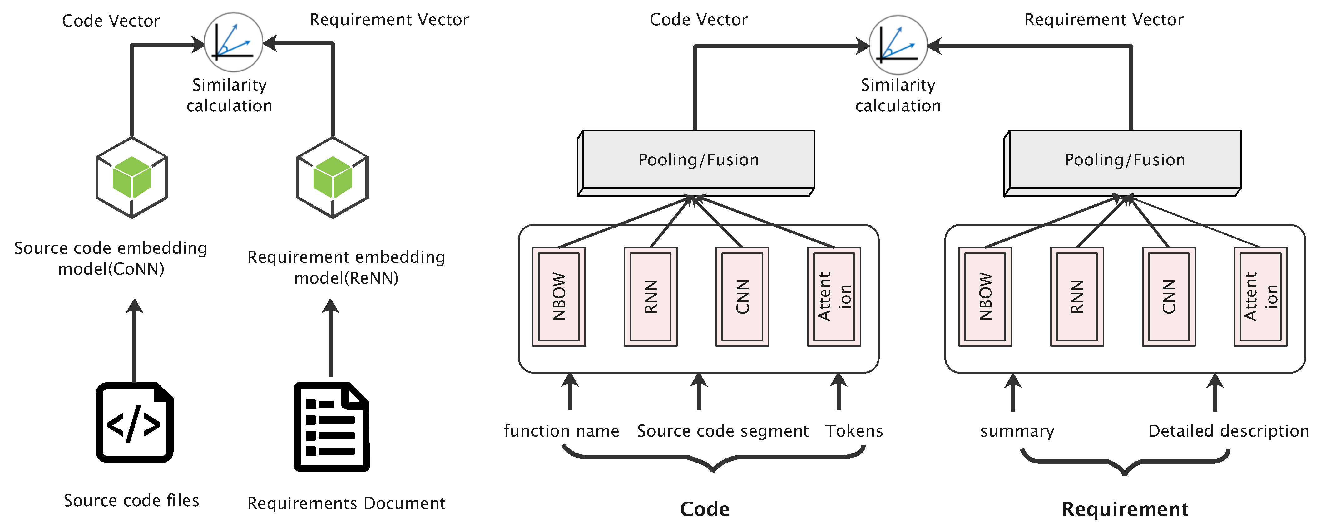
3. Overview of Approach

In view of the powerful representation and feature extraction capabilities of neural networks, this paper proposes a neural-network-based tracing model, RCT, which consists of four layers, as shown in Figure 1. These are the input layer, the embedding layer, the pooling/fusion layer, and the comparison layer. The source code and requirements are finally embedded into a unified vector space after passing through these four layers, and the similarity between them is compared.

Firstly, the input layer is the lowest level of the model and is used to input each requirement from the requirements document and the functions from the source code file into the tracing model. Each input requirement contains an overview and a detailed description of the requirement. The source code file input consists of function names, source code segments, and preprocessed tokens: (1) A function name is the name that defines a function. For each function, we extract its name and parse it into a sequence of tokens based on camel case or underscore naming. For example, valid_path or validPath would be parsed into valid and path tokens. (2) We extract the entire contents of each Java function body as a segment. (3) For the preprocessing of tokens, we first collect the tokens from the function, split each token according to camel or underscore nomenclature, and remove duplicate tokens. We also remove stop words (e.g., and, in, etc.) and keywords as they often appear in the source code and are indistinguishable. In addition, the functions’ APIs contain important semantic information. We obtain information about the API sequence of a function by parsing the abstract syntax tree (AST). The source code files are stripped of files such as build configurations, binaries, project descriptions, data descriptions, etc. We do not consider third-party files, such as various library files. Instead, the focus is only on the code files created by the developer. The CoNN and ReNN of the embedding layer are used to embed the requirements and source code input into the feature space to obtain the feature vectors, each containing the semantic information of the word. A total of four neural network architectures are chosen: neural bag of words (NBOW), recurrent neural network (RNN), convolutional neural network (CNN), and self-attention model. The performance of each neural network is compared in the subsequent experimental validation to select the optimal embedding model. The third layer is the pooling/fusion layer, where the embedding vectors obtained in the previous layer are fused into a sequence vector using a pooling function, generating a feature vector for each requirement ($Requirementvector$) and a feature vector for each function in the source code file ($Codevector$). The final layer is the comparison layer, which compares the cosine similarity or spatial distance between the software requirements and the feature vectors ($Requirementvector$ and $Codevector$) of the source code, and constructs a tracing relationship between the vectors with high similarity or short spatial distance. Next, we show how to use neural networks to transform software requirements and source code into feature vectors and build links between these feature vectors by calculating their similarities.

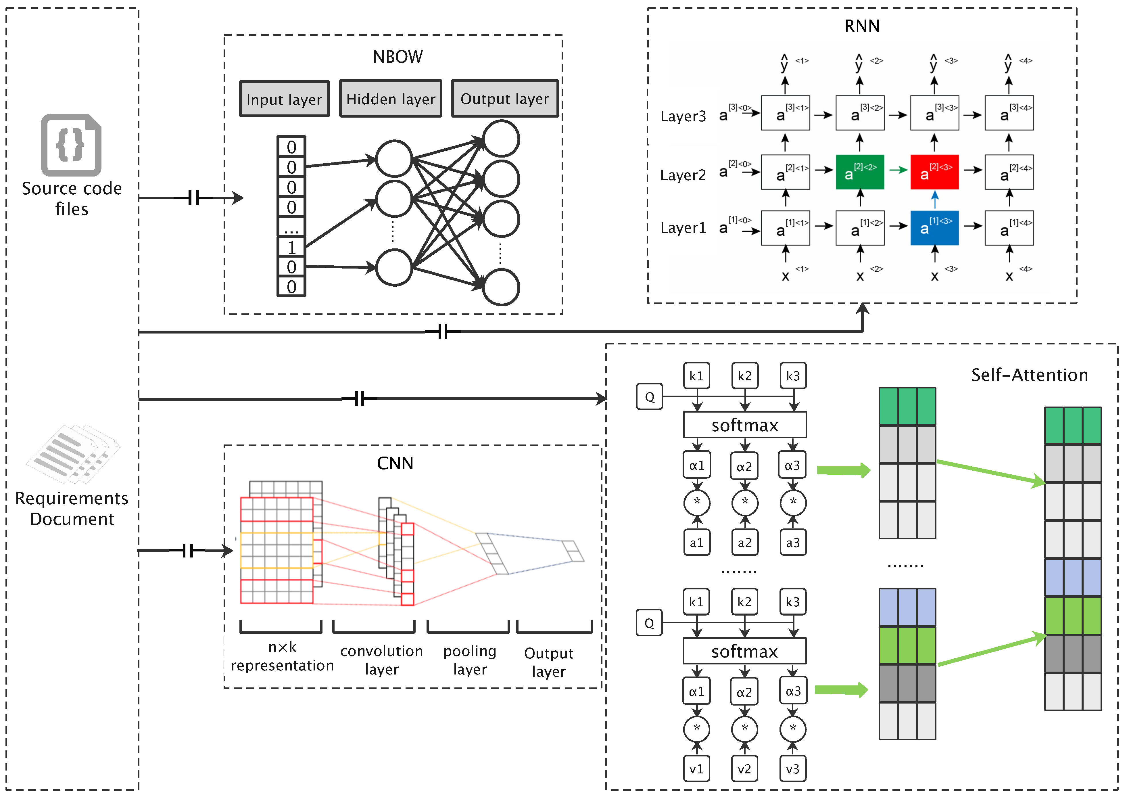
3.1. Neural Network Structures

Many existing deep learning models and related training methods have origins in studying artificial neural networks (ANNs). Inspired by advances in neuroscience, artificial neural networks have been designed to approximate the human brain’s complex functions by connecting a large number of computational units in a multilayer structure. Based on ANNs, deep learning models have a more complex network structure with more connected layers. Data features can be better represented from the more complex structures, which often allows more information to be extracted than more traditional machine learning techniques. In traditional machine learning techniques, human expertise is required to select data features for training. Backpropagation [37] is an effective method for training deep neural networks that indicates how a neural network should adjust its internal parameters to better compute the representation in each layer. Furthermore, as RCT is designed to create trace links and evaluate different neural network models, we will explain in depth how these techniques extract semantic information from software requirements and source code.

The tracing model’s most important component is converting the software requirements and source code into feature vectors via a neural network, which extracts the semantic information in the software requirements and source code as input to the comparison layer. The network consists of the embedding layer and the pooling/fusion layer. Due to the differences in the textual composition of software requirements and source code, the words included in these texts are only partially semantically relevant. Neural network models can be more accurate if they can process the contextual relationships and remove distracting words to obtain the textual semantics of sentences, paragraphs, and documents. Source code is a list of readable instructions under specific authoring rules and has a much more complex structure than text written in natural language. Source code files contain many file names, function names, variable names, etc. Some of these contain the textual semantics of the source code, while others are related to the implementation of functions. In this paper, four embedding neural network models are selected, namely, neural bag of words (NBOW), recurrent neural network (RNN), convolutional neural network (CNN), and self-attention network. The overall structure of the word embedding layer is shown in Figure 2.

3.1.1. Embedding Model Based on NBOW

The bag of words (BOW) model is initially used in text classification to represent documents as a vector of features. The basic idea is that a text is a collection of words, ignoring word order, syntax, and grammar. Each word in the text is independent, and each document is viewed as a bag of words. The neural bag of words model is a fully connected feedforward network with BOW input. It maps the text X (a sequence of words) to one of k output labels, where each vector has dimension d. The input used in this paper is the one-hot vector. The one-hot encoding represents a word in the text by a vector of word number dimensions, where the value corresponding to the word is 1, and the other values are 0. For each word $w\in X$ in this word sequence, its corresponding word vector is $v_w$. Based on the input set of vectors, their average is taken as the hidden vector z. Preliminary experiments indicate that averaging outperforms the vector sum used in NBOW from Kalchbrenner et al. [38].

$$z=\frac{1}{\left|X\right|}\sum _{w\in X}{v}_w.$$

(1)

This average vector z is then fed into a fully connected layer to obtain the probability of the output label. Its hidden layer consists of linear cells and does not require an activation function. The vector dimension of the output layer is the same as the dimension of the input layer and uses $softmax$ regression.

$$\widehat{y}=softmax(W_{l}z+b).$$

(2)

where $W_l$ is a matrix of $k\times d$, b is a bias vector, and $softmax\left(x\right)=exp\left(x\right)/{\sum }_{j=1}^{k}exp\left(x_j\right)$. The NBOW model can be trained using the stochastic gradient descent algorithm, where the loss function can be used as a cross-entropy function. Additional fully connected layers can be added into the NBOW model to form deep averaging networks (DANs) [39]. Both CBOW and skip-gram models [40] can be seen as an improvement of the neural bag-of-words model, although they are of opposite mindsets. The training input to the CBOW model is the contextually relevant words, and the output is the word vector of this particular word. The input to the skip-gram model is a particular word, and the output is the contextual word vector corresponding to it. The neural bag-of-words model embeds the vocabulary, as shown in Equation (3). Pooling functions later combine the feature vectors $e_1,e_2,...,e_n$.

$$e_1,e_2,...,e_n=embedding\left(wordsinrequirementorsourcecode\right).$$

(3)

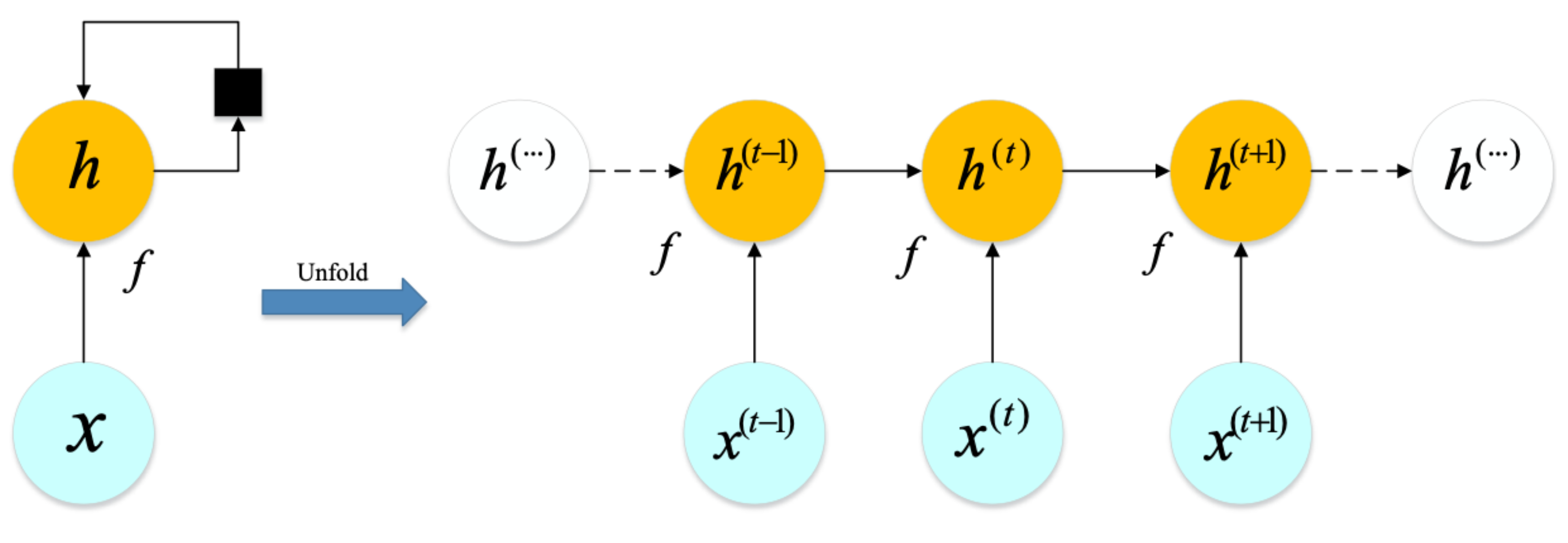
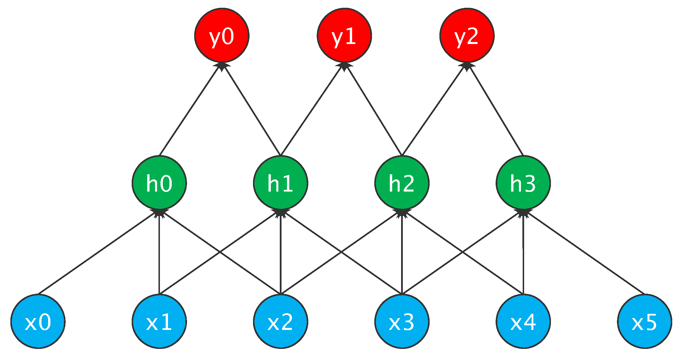
3.1.2. Embedding Model Based on RNN

Recurrent neural networks (RNNs) are mainly used for tasks related to natural language processing. In the case of textual information, the fact that the nodes of a conventional neural network are not connected at each layer means that such networks cannot deal with, for example, temporal problems. Because these neural networks can only process the content of the current input word, they need a reference to the context of the word and therefore miss a lot of information during training. Recurrent neural networks have neuronal feedback connections, allowing the network to store information about the most recent input data in a stimulated form (short-term memory). In Figure 3, it is clear that information about the state of the network at the last moment will act on the output computed at the next moment. We use a function $g^{\left(t\right)}$ to represent the computation after t steps of expansion.

$$h^{\left(t\right)}=g^{\left(t\right)}(x^{\left(t\right)},x^{(t-1)},x^{(t-2)},\dots ,x^{\left(2\right)},x^{\left(1\right)})=f(W{h}^{(t-1)}+U{x}^{\left(t\right)}+b).$$

(4)

where $W,U$ is the transformation matrix, b is the bias vector, and f is the nonlinear activation function, e.g., the hyperbolic tangent function $tanh\left(z\right)=(e^{\left(z\right)}-e^{(-z)})/(e^{\left(z\right)}+e^{(-z)})$.

Figure 3 shows a single-layer RNN network. The RNN network in Figure 2 is a stack of single-layer RNNs in a multilayer network, where $x^{<1>},\dots ,x^{<4>}$ is the input to the RNN network. In this paper, this is a vector of words from software requirements or source code text. ${\widehat{y}}^{<1>},\dots ,{\widehat{y}}^{<4>}$ is the output of the RNN. The output of the red neural unit is related to the green and blue neural units, and the equations are shown in (5). Since the RNN can store information on input data from the most recent time period (short-term memory), $y^{<4>}$ contains the semantic information of these words.

$$a^{\left[2\right]<3>}=g(W_a[a^{\left[2\right]<2>},a^{\left[1\right]<3>}]+b_a).$$

(5)

A significant problem with RNN models is that when there are long dependent terms in the sequence, the network degrades because of the gradient explosion or disappearance during backpropagation [41]. Using GRU or LSTM [42] can better solve the problem of gradient explosion and gradient disappearance. LSTM remembers information by adding unit states and reduces the possibility of gradient disappearance and gradient explosion by using input gates, output gates, and forget gates. This enables both short-term and long-term dependency problems to be dealt with. LSTM has been repeatedly applied to solve semantic relatedness tasks and has achieved convincing performance [13,43]. This paper, therefore, uses the LSTM network as a superordinate replacement for the RNN network. Since the LSTM network contains a vector of memory units in each cell, remembering longer history information is its default behavior rather than something they struggle to learn. Each LSTM unit contains an input gate $i_t$, an output gate $o_t$, and a forget gate $f_t$, and they are each calculated as shown below.

$$i_t=\sigma (W_i{x}_t+U_i{h}_{t-1}+b_i).$$

(6)

$$o_t=\sigma (W_o{x}_t+U_o{h}_{t-1}+b_o).$$

(7)

$$f_t=\sigma (W_f{x}_t+U_f{h}_{t-1}+b_f).$$

(8)

To update the information in the memory cell, a memory candidate vector ($\widetilde{c_t}$) is first calculated using the $tanh$ function. The memory unit $c_t$ is then obtained from the sum of the candidate vector ($\widetilde{c_t}$) passing through the input gate and the previous memory unit $c_{t-1}$ passing through the forget gate. The purpose of this memory candidate is to control how much of the candidate vector and information from the previous memory cell needs to be “remembered”.

$$\widetilde{c_t}=Tanh(W_c{x}_i+U_c{h}_{t-1}).$$

(9)

$$c_t=f_t\odot c_{t-1}+i_t\odot \widetilde{c_t}.$$

(10)

Finally, the LSTM unit calculates its output $h_t$ with an output gate as follows:

$$h_t=o_t\odot Tanh\left(c_t\right).$$

(11)

3.1.3. Embedding Model Based on Self-Attention

The self-attention model is one of the building modules in Transformer, a new network architecture proposed by Google in 2017 [44]. Encoder–decoders were previously implemented based on convolutional or recurrent neural networks. On the other hand, the Transformer is implemented entirely based on the attention mechanism. Their experiments on two machine translation tasks show that the model is easier to parallelize and requires less training time. This is because the traditional Seq2Seq model has difficulty processing long sequences of sentences and is not parallelizable.

The attention mechanism allows the neural network to learn the differences and weights of words in a sentence, which can improve the accuracy of the neural network model. The self-attention network used in this paper consists of several parallel attention layers, and the attention mechanism is an addressing process. Given a task-related queryvector Q, its attention distribution with respect to the key is computed and attached to the value.

The process is divided into three steps: (1) Information input: the $Q,K,V$ is represented by $X=[x_1,x_2,\dots ,x_n]$ as the input weight vector. For example, a sequence contains four words, then their embedding vectors are $a_1,a_2,a_3,a_4$. Each vector is multiplied by a different transformation matrix $W_q,W_k,W_v$, for example, using the vector $a_1$ to obtain $q_1,k_1,v_1$, respectively. (2) Calculate the attention distribution: compute the correlation by the dot product of Q and K, and compute the attention weight ${\alpha }_i=softmax\left(s(k_i,q)\right)=softmax(k_i^{T}q/\sqrt{d_k})$ by $softmax$. Attention is used to match the similarity of these two vectors. For example, computing $q_1$ and $k_2$ yields ${\alpha }_{1,2}$. Since the value of $q\times k$ increases as the dimensionality increases, dividing by the value of $\sqrt{d_k}$ is equivalent to normalization [45]. Next, all the computed ${\alpha }_{i,j}$ values are passed through the $softmax$ layer to obtain ${\tilde{\alpha }}_{i,j}$. The attention weight ${\alpha }_i$ is used to explain how much attention is paid to the ith attention weight information in the contextual query $q_i$. For example, when computing the spatial vector for a software requirement “read an object from an XML file”, the attention score for each word in the sentence is first computed, which ultimately determines the attention devoted to each part of the sentence when encoding the word embedding. (3) The output vector is computed from the attention weights. Since ${\tilde{\alpha }}_{i,j}$ has been obtained, it is multiplied and summed with all $v_j$. For example, $o_1={\sum }_j{\widehat{\alpha }}_{1,j}{v}_j$. Thus, it can be seen that $o_1$ is generated, taking into account the semantic information of the whole sentence.

To summarize the above steps: the input matrix is $I\in \mathbb{R}(d,N)$ containing N-dimensional vectors after word embedding. The I are multiplied by three different transformation matrices $W_q,W_k,W_v$ to obtain the intermediate matrices $Q,K,V\in \mathbb{R}(d,N)$. Transpose K and multiply it with Q to obtain the attention matrix $A\in \mathbb{R}(N,N)$, which is then subjected to $softmax$ to obtain $\widehat{A}\in \mathbb{R}(N,N)$. It is multiplied by the matrix V to obtain the final output matrix $O\in \mathbb{R}(d,N)$. The formulae are shown in (12) and (13).

$$\widehat{A}=softmax\left(A\right)=K^T·Q.$$

(12)

$$O=V·\widehat{A}.$$

(13)

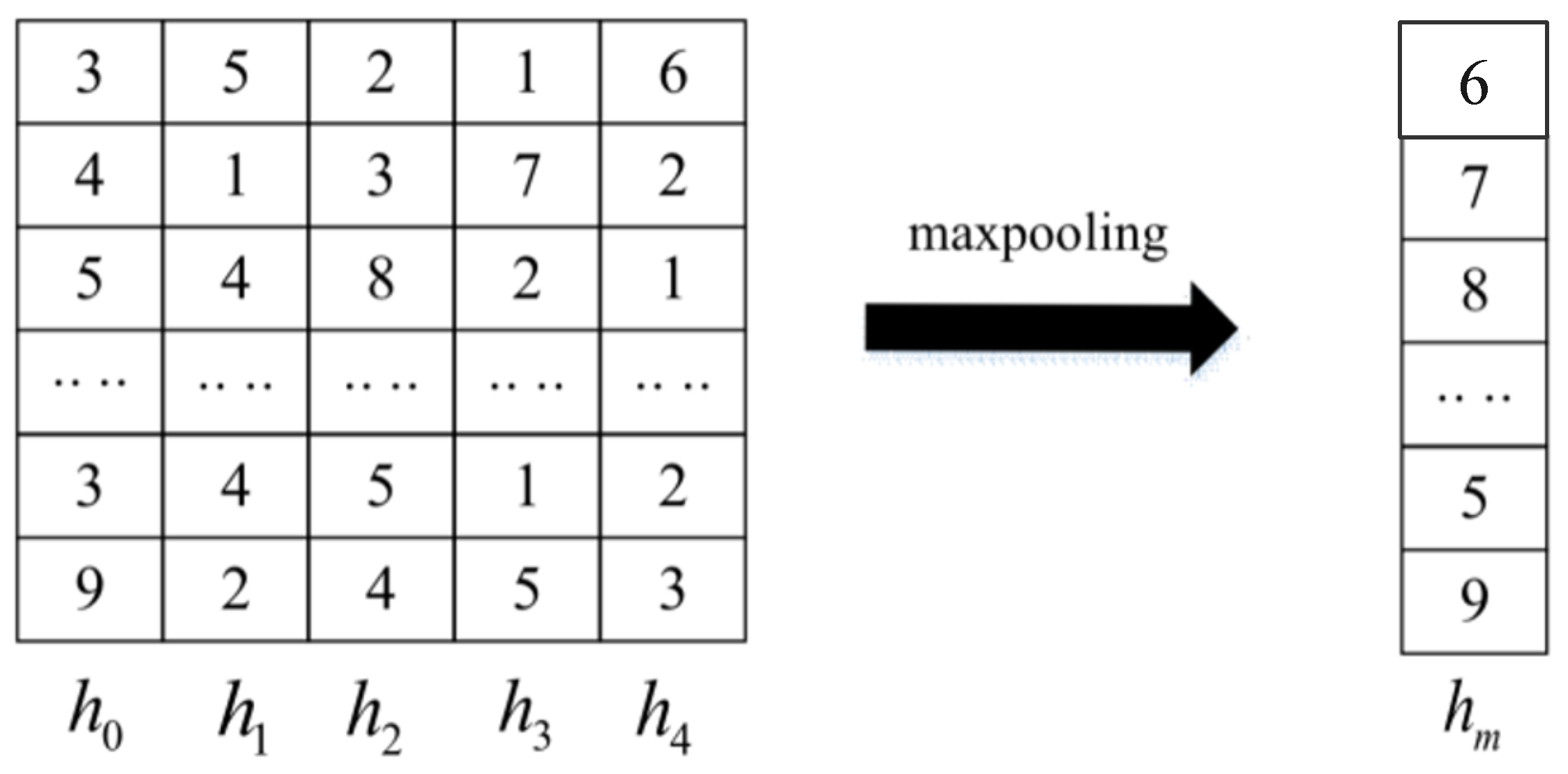
3.2. Embedding Model Based on CNN

Convolutional neural networks (CNNs) can learn local features and assume that these features are not constrained by absolute position. In the field of natural language processing, it is mainly used for lexical annotation, named entity recognition, etc. [38,46]. The convolutional layer applies a one-dimensional filter to each row of features in the sentence matrix. The same filter at each position in the sentence as the n-gram convolution allows features to be extracted independently. The model of the convolutional neural network is shown in Figure 4. For the green nodes $h_0=f(W(x_0,x_1,x_2)+b)=f(w_0{x}_0+w_1{x}_1+w_2{x}_2+b),h_1=f(W(x_1,x_2,x_3)+b)=f(w_1{x}_1+w_2{x}_2+w_3{x}_3+b)$. In each layer of the neural network, the value of W is shared. This leads to the following two characteristics of convolutional neural networks [47].

1.

Sparse connection: This enables each neuron in the neural network to focus on acquiring local features.

2.

Weight sharing: It increases efficiency by reducing the number of parameters to be learned and allows the model to be generalized.

CNN for natural language processing can be divided into single-convolutional layer CNN and multiconvolutional layer CNN, so the convolution used can be 1d, 2d, or even 3d. A single convolutional layer CNN extracts token features from word embeddings and learns sentence features through a layer of convolutional neural networks. The token and sentence features are then fed back into the neural network to predict the relationship between two given words in a sentence. A single convolutional layer CNN used by RCT is illustrated in Figure 2, and the structure is defined and applied to the semantic modeling of sentences, which can handle input sequences of different lengths. The layers in the network are divided into a one-dimensional convolutional layer and a dynamic $k-max$ pooling layer. Assuming that there are n words in a sentence and that the dimension of the word vector is k after each word is embedded, the input to the CNN network is an $n\times k$- dimensional matrix. We set a sliding window of length h, i.e., the number of words in the vertical direction. Using this sliding window to slide through the entire matrix, the window size of the convolution is $h\times k$, after which the vector c corresponding to one feature is calculated by Equation (14). The feature $c_i$ is generated from a window consisting of the words $x_{i:i+h-1}$. w is the weight and b is the bias.

$$c_i=f(W·x_{i:i+h-1}+b).$$

(14)

where the weights obtained from training in W correspond to feature detectors that learn to recognize specific classes of $n-grams$. $n-grams\le h$, where h is the width of the sliding window. A wide convolutional sliding window h is preferable to a narrow convolutional sliding window h. Wide convolution ensures that all weights in the filter reach the entire sentence, including words at the edges. This is particularly important when h is set to a relatively large value, such as 8 or 10. In addition, wide convolution ensures that applying the sliding window filter to the input sentence s always produces a valid nonempty result c, independent of the width h and sentence length n. Multiple feature vectors can be generated by varying the size of h, and the set of these vectors is called a $Featuremap$. $Featuremap\mathbf{c}=[c_1,c_2,\dots ,c_{n-h+1})]$. This $Featuremap\mathbf{c}$ is then passed through a dynamic $k-max$ pooling layer. The dynamic $k-max$ pooling layer is a morphing and generalization of $maxpooling$. The max pooling operator is a nonlinear subsampling function that returns the maximum of a set of values. The dynamic $k-max$ pooling layer has been improved in two ways. Firstly, for linear sequences of values $k-max$, the pooling layer will return a subsequence of k maxima in the sequence rather than a single maximum. Secondly, the pooling parameter k can be dynamically chosen by a function of other aspects, such as input. The pooling layer also solves the problem of variable-length sentence inputs. The final output layer is a fully connected layer + a $softmax$ layer for different NLP tasks, using dropout or L2 regularization to avoid overfitting the network [48].

3.3. Requirement and Source Code Feature Vector Generation

Based on these neural networks, it is possible to convert software requirement vocabularies or sentences and source code tokens into spatial vectors. RCT fuses these distributed feature vectors into a single feature vector representing the semantic information of the software requirements or source code functions through pooling or fully connected neural networks. Pooling-related techniques are also gaining interest in natural language processing. The pooling layer is responsible for maintaining invariance in the event of data changes and perturbations. A pooling operation is generally divided into two steps. First, the pooling operator scans the feature map or feature vector and aggregates the feature information within each local region. Information aggregation can enhance robustness against data translation and change to a certain extent. For example, an average or maximum pooling operation takes a local region’s average or maximum value. Secondly, the downsampling operation retains only a portion of the aggregated data for each feature channel and skips the rest with a fixed sampling step. A larger matrix of feature vectors is obtained after passing through the neural network for software requirements and source code. A simplified natural approach is used to statistically aggregate the data by calculating the mean, maximum, and L2 parity of particular values. Pooling results in fewer features and fewer parameters. Taking $Maxpooling$ as an example, $Maxpooling$ captures the most important features in each region, i.e., the features with the maximum values, as shown in Figure 5.

In RCT, $Maxpooling$ extracts the most important features in the vector for representing semantic information. The idea is to capture the most important feature for each feature vector—the feature with the highest value [49]. This pooling scheme naturally deals with variable sentence lengths. Thus, the source code is embedded to obtain a feature vector $\overrightarrow{h_M}$ for function names, a feature vector $\overrightarrow{h_{CS}}$ for source segment, and $\overrightarrow{h_{CT}}$ for tokens in the preprocessed source generation. The software requirements are passed through the embedding layer to obtain feature vectors, $\overrightarrow{h_{RS}}$, $\overrightarrow{h_{RD}}$, representing the requirement summary and description, respectively. After passing through the pooling network, the output vectors are calculated as shown in (15) and (16), respectively, where ⊕ denotes the pooling network or fully connected network, the final $Codevector$ and $Requirementvector$ represent the software requirements and the source codes. Theyare generated through the pooling network.

$$codevector=\overrightarrow{h_M}\oplus \overrightarrow{h_{CS}}\oplus \overrightarrow{h_{CT}}.$$

(15)

$$codevector=\overrightarrow{h_{RS}}\oplus \overrightarrow{h_{RD}}.$$

(16)

3.4. Similarity Calculation and Model Training

The software requirement and source code functions pass through the embedding and pooling/fusion layers to obtain a source code feature vector ($Codevector$) and a requirement feature vector ($Requirementvector$) containing their semantic information, respectively. These vectors are then used as input to the comparison layer, the final layer of the RCT model. It compares the $Codevector$ with the $Requirementvector$ and calculates the similarity between them, generating links between the requirements and the source code for the top-ranked requirements. The final traceability links between requirements and code are constructed and used to analyze the impact of requirements changes on the code or in software development and testing. Commonly used vector similarity calculation methods are shown in Equations (17)–(19).

$$PearsonCorrelationCoefficient:P_{sim}(x,y)=\frac{n\sum x_i{y}_i-\sum x_i\sum y_i}{\sqrt{n\sum {x_i}^2-{(\sum x_i)}^2}\sqrt{n\sum {y_i}^2-{(\sum y_i)}^2}}.$$

(17)

$$EuclideanDistance:E_{xim}(x,y)=\frac{1}{\sqrt{\sum {(x_i-y_i)}^2}+1}.$$

(18)

$$CosineSimilarity:C_{sim}(x,y)=\frac{\sum x_i{y}_i}{\sqrt{\sum x_i^2}\sqrt{\sum y_i^2}}.$$

(19)

Once a tracing neural network model has been built, training the neural network model is one of the key issues to be considered, as it is directly related to the accuracy of the final tracing relationship established. Traditional classification models can use exponential loss, Hinge loss, and cross-entropy loss functions. However, these functions are not suitable for this paper’s study because our tracing model aims to obtain the similarity between software requirements and code. In other words, given a code fragment C and a software requirement R, if there is a tracing link between C and R, the model will predict a high similarity; otherwise, a low similarity. Therefore, during training, each training datum is constructed as a triple $<C,R^{+},R^{-}>$: for each code fragment C there is a requirement $R^{+}$ with tracing relationship and a requirement $R^{-}$ without tracing relationship. The final loss function improves on the Hinge loss function. RCT predicts the cosine similarity between $<C,R^{+}>$ and $<C,R^{-}>$ and minimizes the ranking loss [50]. This is shown in Equation (20).

$$L\left(\theta \right)=\sum _{<c,R^{+},R^{-}>\in TS}max(\epsilon ,\lambda -sim(c,R^{+})+sim(c,R^{-})).$$

(20)

where $\theta$ represents the parameters of the model, $TS$ represents the training set, and the similarity between the software requirements and the source code is $sim(C,R^{+})$. $sim(C,R^{-})$ can be calculated using Equations (17)–(19). We use an initial value of $\lambda$ minus the similarity between $sim(C,R^{+})$ and add the similarity between $sim(C,R^{-})$ as the final loss function. It is not necessary to mark the similarity between software requirements and source code in each piece of data. This is because as the model is trained, this ranking loss function $L\left(\theta \right)$ will gradually increase the cosine similarity between software requirements and source code with tracing relationships and, conversely, decrease for those without tracing relationships. The RCT thus trained will result in a high similarity between requirement-code pairs with tracing relationships and a high ranking when constructing trace links. Requirement-code pairs without tracing relationships are less similar and are ranked lower. In addition, to prevent the loss function from being less than 0, a decimal “$\epsilon$”, which is slightly larger than 0, is used as a lower bound for the loss function.

4. Experiment Setup

4.1. Subject Programs and Metrics

This paper uses the natural language description-code corpus [51] provided by Microsoft as a training set. The corpus contains thousands of Java functions and their corresponding natural language descriptions, i.e., $<C,R^{+}>$. To obtain the $<C,R^{+},R^{-}>$ needed for training, we manually add a natural language description $R^{-}$ that does not have a tracing relationship to form $(C,R^{-})$. The tracing neural network is trained using the training set and the loss function $L\left(\theta \right)$. The validation and test set use traceability links between issues (including requirements, bug reports, and code change history) and the entire project source code (from 33 open source projects) provided by Rath et al. [52]. We select data with the issue types feature, new feature, feature request, improvement, and enhancement, then remove data with the issue types bugs, tasks, patches, etc. This means that the focus is only on new requirements for the product and enhancements to existing requirements. Each piece of data in this dataset contains a brief and detailed description of the requirement (for example, a new feature in the archiva project is outlined as “Repository purge feature for snapshots”, and the detailed description is “We need a way to purge a repository of snapshots older than a certain date, (optionally retaining the most recent one) and fixing the metadata”) and traceability links between it and the code files. A piece of data is $<R,C_1{1}^{+},C_2^{+},\dots ,C_n^{+}>$. A requirement R and the source code $C_n^{+}$ have tracing relationships. This dataset is stored in a relational database in SQLite, and the data in this database are filtered and integrated to obtain the final validation set. Once the model is trained, each requirement R is fed into the tracing neural network, and the number of code functions that the model predicts to have tracing relationship $C_n^{+}$ (true positive) is counted, which provides a visual representation of how well the tracing model performs. Theoretically, RCT can construct traceability links between source code and requirements written in any programming language. For this paper, only Java projects are used as experimental objects, so 18 projects developed in Java are selected from these 33 projects to verify the model performance. The specific project names and the number of requirements they contain, the number of source code files, and the number of traceability links between requirements and source code files are shown in

Table 2. Experimental data.

Project Name	Requirement Number	Number of Source Files	Number of Traceability Links
archiva 1	174	750	3028
cassandra 2	1992	2203	22,399
derby 3	980	2849	14,736
drools 4	654	4342	29,399
errai 5	152	3815	2630
flink 6	1177	5366	22,082
groovy 7	736	1376	2693
hbase 8	2169	3429	24,986
hibernate 9	819	9178	23,542
hive 10	1738	5544	15,468
kafka 11	257	1564	3156
keycloak 12	505	4343	21,820
maven 13	357	966	2782
railo 14	167	2788	1147
spark 15	513	857	2338
switchyard 16	334	2954	12,719
teiid 17	768	2 269	23,941
zookepper 18	229	603	2457
total	13,721	55,196	231,323

¹https://doi.org/10.7910/DVN/PDDZ4Q/SYQTC9; ²https://doi.org/10.7910/DVN/PDDZ4Q/E9PAND; ³https://doi.org/10.7910/DVN/PDDZ4Q/I74GST; ⁴https://doi.org/10.7910/DVN/PDDZ4Q/BFEOXT; ⁵https://doi.org/10.7910/DVN/PDDZ4Q/OPG8N9; ⁶https://doi.org/10.7910/DVN/PDDZ4Q/KFMXVI; ⁷https://doi.org/10.7910/DVN/PDDZ4Q/PLQP8O; ⁸https://doi.org/10.7910/DVN/PDDZ4Q/NO3KD8; ⁹https://doi.org/10.7910/DVN/PDDZ4Q/0ITQ9A; ¹⁰https://doi.org/10.7910/DVN/PDDZ4Q/CEUQJR; ¹¹https://doi.org/10.7910/DVN/PDDZ4Q/LYZAIU; ¹²https://doi.org/10.7910/DVN/PDDZ4Q/0IMEHO; ¹³https://doi.org/10.7910/DVN/PDDZ4Q/TFY2J1; ¹⁴https://doi.org/10.7910/DVN/PDDZ4Q/AVY9DX; ¹⁵https://doi.org/10.7910/DVN/PDDZ4Q/U2DEMZ; ¹⁶https://doi.org/10.7910/DVN/PDDZ4Q/HS3IF6; ¹⁷https://doi.org/10.7910/DVN/PDDZ4Q/J8NZXZ; ¹⁸https://doi.org/10.7910/DVN/PDDZ4Q/OVRUZW (accessed on 24 May 2019).

.

This experiment uses two common metrics to measure the performance of neural networks in constructing traceability links between software requirement and code, namely, $Recall@k$ and mean reciprocal rank (MRR), which are widely used in recommendation algorithms, information retrieval, etc. [53,54,55].

• The $Recall@k$ metric measures the percentage of correct relevant results among the first k results returned by each query or prediction [44], which is calculated as shown in Equation (21), where $TP@k$ is the correct relevant results among the first k results and $FN@k$ is the correct results that were not detected in the first k results.

  $$Recall@k=\frac{TP@k}{TP@k+FN@k}.$$

  (21)
  Because a requirement may be related to multiple code files in the software, a higher value of $Recall@k$ indicates a better performance in constructing traceability links between the software requirements and the source code.
• $Meanreciprocalrank\left(MRR\right)$ [44,50] is the position of the first relevant result $firs{t}_q$ in the ranked list obtained based on each query or search q, calculated as shown in (22):

  $$MRR=\frac{1}{\left|Q\right|}\sum _{q=1}^{\left|Q\right|}\frac{1}{firs{t}_q}.$$

  (22)

4.2. Experiment Process

We use the natural language description-code corpus provided by Microsoft as the training set. The traceability link data provided by Rath et al. from the open-source project mentioned above are used as validation and test data. These advantages are twofold: (1) there is no overlap between the training set and the validation and test sets, which allows for better evaluation of the tracing model’s properties and avoids errors in the test results due to the same data; (2) the projects in Rath et al.’s dataset are real open-source projects, and their job is to collect the traceability link data from these projects. Therefore, using them as a validation or test set gives an idea of how well the tracing model generalizes to real scenarios. These data are preprocessed as input to the tracing model. The processing of the requirements is relatively straightforward, extracting their general and detailed descriptions and removing the stop words. The source code is processed by first traversing all the project files, and RCT uses TreeSitter (a generic parser from Github) to compile the functions in these projects and extract the function name, function segment, and each token in them. Source code and natural language requirements are embedded in the same vector space. The similarity between $requirementvector$ and $codevector$ is calculated to determine whether there are traceability links. After the tracing model is trained, we use the validation and test set data to compare the performance of each neural network to select the best embedding network. Finally, we compare RCT with previous link-constructing methods (LSA, VSM, BM25, TraceNN, Poirot (PN)). The overall process is shown in Figure 6 below.

The implementation of the RCT model is written in Python. The neural network’s hyperparameters are continuously tuned during training to achieve the best combination of parameters, with the best average over all the source items, as the optimal parameter configuration, as shown in

Table 3. Tracing network configuration.

Network Type	NBOW, RNN, CNN, Self-Attention
Batch Size	1000
Learning Rate	0.01
Learning Rate Decay	0.98
Code Max Num Tokens	200
Query Max Num Tokens	30
Dropout Keep Rate	0.9
Max Epoch	500
Optimizer	Adam

. The “Code Max Num Tokens” and “Query Max Num Tokens” are the maximum length of each code segment and each requirement input into the network. Tokens after the maximum length are removed. The performance of the resulting tracing model is guaranteed to converge under the optimal parameter configuration.

5. Results

In order to evaluate the effectiveness of the tracking network, the following two questions (RQ) are investigated.

1.

RQ1: Which neural network model in RCT can obtain better results for constructing traceability links between software requirements and source code?

2.

RQ2: Is RCT better than other methods of constructing traceability links between software requirements and source code?

5.1. RQ1 Comparative Experimental Analysis

To answer RQ1, this paper uses four neural networks (NBOW, RNN, CNN, and self-attention) to embed software requirements and source code, and conducts comparative experiments using training datasets. The experimental results are shown in Figure 7.

Figure 7 shows the change in the loss function values of the model and the MRR values as the training process continues to advance. The overall performance of the neural bag-of-words model (NBOW) changes less as the training process progresses. In addition, the convolutional neural network (CNN), recurrent neural network (RNN), and self-attention models gradually decrease the value of the loss function and increase the value of MRR as the training process progresses. CNN has the slowest convergence rate and the worst MRR value in the validation set. Self-attention has the best performance on the validation set and performs slightly better than RNN.

To further compare the performance of each neural network in various real-world projects, we use 18 practical projects as the test set. The testing metrics are $Recall@10$, $Recall@30$, and $Recall@50$. In the context of constructing traceability links, recall is the key measure because it shows the percentage of correct links between requirements and code that the model can find. A high recall means there is little likelihood that our model will miss a correct link, which is in line with the ultimate goal of traceability research. It is not appropriate to use $precision@k$ as a metric because the number of source codes corresponding to each software requirement is different. Once RCT has found all the source code for a requirement, increasing the value of k at this point will cause the $Precision@k$ value to decrease, resulting in inaccurate results. For example, all ten source code functions related to a requirement are in the top 10 prediction results, showing that RCT can construct accurate traceability links for that requirement. $Recall@10$, $Recall@30$, and $Recall@50$ all have a value of 1; however, $Precision@10$, $Precision@30$, and $Precision@50$ have values of 1 (10/10), 0.333 (10/30), and 0.2 (10/50), respectively. It can be seen that $Precision@k$ does not reflect the performance of RCT; therefore, it is better to use $Recall@k$ as a metric.

Table 4. Performance of 4 neural network models under $Recall@10$.

Project Name	NBOW	CNN	RNN	Self-Attention
archiva	0.281	0.443	0.449	0.298
cassandra	0.419	0.384	0.411	0.416
derby	0.520	0.213	0.622	0.521
drools	0.325	0.255	0.312	0.334
errai	0.358	0.334	0.365	0.337
flink	0.349	0.333	0.343	0.340
groovy	0.736	0.727	0.709	0.743
hbase	0.398	0.381	0.380	0.382
hibernate	0.443	0.434	0.460	0.461
hive	0.419	0.401	0.392	0.410
kafka	0.367	0.333	0.396	0.343
keycloak	0.357	0.316	0.340	0.326
maven	0.485	0.434	0.509	0.481
railo	0.434	0.397	0.409	0.397
spark	0.598	0.476	0.538	0.554
switchyard	0.484	0.492	0.288	0.502
teiid	0.290	0.301	0.293	0.309
zookepper	0.480	0.481	0.459	0.479

,

Table 5. Performance of 4 neural network models under $Recall@30$.

Project Name	NBOW	CNN	RNN	Self-Attention
archiva	0.483	0.532	0.579	0.553
cassandra	0.543	0.540	0.531	0.546
derby	0.639	0.458	0.675	0.605
drools	0.480	0.419	0.427	0.452
errai	0.511	0.516	0.476	0.519
flink	0.487	0.461	0.487	0.502
groovy	0.793	0.768	0.788	0.768
hbase	0.516	0.511	0.518	0.523
hibernate	0.581	0.562	0.614	0.590
hive	0.562	0.552	0.544	0.536
kafka	0.503	0.514	0.504	0.527
keycloak	0.484	0.494	0.497	0.511
maven	0.595	0.570	0.611	0.604
railo	0.569	0.510	0.590	0.527
spark	0.700	0.614	0.633	0.682
switchyard	0.714	0.702	0.572	0.741
teiid	0.439	0.418	0.437	0.448
zookepper	0.621	0.609	0.586	0.640

and

Table 6. Performance of 4 neural network models under $Recall@50$.

Project Name	NBOW	CNN	RNN	Self-Attention
archiva	0.574	0.651	0.629	0.621
cassandra	0.620	0.630	0.617	0.636
derby	0.713	0.767	0.683	0.676
drools	0.544	0.548	0.526	0.550
errai	0.561	0.596	0.557	0.587
flink	0.578	0.572	0.579	0.599
groovy	0.812	0.800	0.821	0.799
hbase	0.604	0.595	0.594	0.610
hibernate	0.665	0.639	0.690	0.647
hive	0.638	0.625	0.620	0.625
kafka	0.610	0.625	0.593	0.670
keycloak	0.564	0.580	0.612	0.586
maven	0.677	0.647	0.688	0.662
railo	0.661	0.558	0.622	0.601
spark	0.735	0.701	0.700	0.720
switchyard	0.822	0.740	0.701	0.838
teiid	0.517	0.499	0.533	0.599
zookepper	0.683	0.692	0.677	0.723

show the significant variation in the evaluation metric $Recall@k$ between projects. They also verify that there is a large variation in the number of traceability links for different requirements. The results for each neural network on the test set are consistent with the results using $MRR$ as the evaluation metric on the validation set. NBOW performs best under the $Recall@10$ metric (with the best performance on 7/18 projects, average $Recall@10$ is 0.430); self-attention performs best under the $Recall@30$ metric (with the best performance on 9/18 projects, average $Recall@10$ is 0.571) and the $Recall@50$ metric (with the best performance on 8/18 projects, average $Recall@50$ is 0.687). In total, self-attention has the best performance (best performance on 22/54 projects, average is 0.561) when all of the above results are tallied. This also shows that the performance of each neural network on the test set is consistent with the performance results on the validation set. The performance of CNN is the worst in $Recall@10$ (0.396) and $Recall@30$ (0.542). Therefore, CNN has the worst performance (average is 0.524) when all of the above results are tallied.

The best performance achieved by self-attention is explainable. This is because in constructing software traceability, the goodness of the remote dependencies between sequences in the learned text determines the final prediction performance. A key factor affecting the ability to learn such dependencies is the length of the signal’s forward versus backward traversal path in the neural network. The shorter the path between any combination of positions in the input and output sequences, the easier it is to learn remote dependencies. The maximum path length in self-attention is $O\left(1\right)$, in RNN it is $O\left(n\right)$, and in CNN it is $O\left(lo{g}_k^{\left(n\right)}\right)$ [44]. n is the length of the text sequence, and k is the convolutional kernel size. The neural bag-of-words model does not have dependencies between learning sequences. Since the convolutional kernel $k\le n$, the maximum path length in both RNN and CNN is larger than self-attention. In addition, self-attention can accept all vectors as input simultaneously, so, to some extent, self-attention is more efficient than RNN.

In summary, this experiment use several projects and evaluation metrics to compare the performance of each neural network in constructing software traceability. It is verified that self-attention has the best performance results and is thus the most suitable for constructing the links between software requirements and source code.

We also compare the time overhead of each neural network model. In Figure 8, the vertical coordinate is the time required to train or validate the data within a single epoch. The NBOW structure is relatively simple, and the CNN can reduce the time overhead through weight sharing and sparse connections. Self-attention has the best performance but also has more time overhead. However, in practice, when using RCT to construct the requirement-code traceability links, the difference in time overhead is not significant (as can be seen from the time difference in seconds required to perform the validation set analysis). Thus, it does not cause problems for the user due to excessive overhead time. Self-attention is still the best neural network model.

5.2. RQ2 Comparative Experimental Analysis

To answer this question, we compare the performance of RCT with existing automated methods for constructing software tracing links. First, the information retrieval algorithms include LSA, VSM, and BM25. These three methods are chosen for comparison because the LSA and VSM algorithms are the most commonly used information retrieval methods for constructing links between software artifacts. In Vale’s experimental results [10], BM25 achieved the best recall results on the five retrieval methods (CV, LSI, NN, EB, and BM25) when constructing traceability links between software feature-codes. The results of the comparative experiments are shown in

Table 7. Performance comparison of RCT with existing techniques for constructing traceability links under $Recall@50$.

Projects Name	RCT [Self-Attention]	LSA	BM25	VSM	TraceNN	Poirot (PN)
archiva	0.621	0.154	0.102	-	0.374	0.201
cassandra	0.636	0.234	0.070	-	0.432	0.181
derby	0.676	0.247	-	-	0.411	0.112
drools	0.550	0.188	-	-	0.387	0.231
errai	0.587	0.191	0.128	-	0.365	0.215
flink	0.599	0.188	0.166	-	0.401	0.224
groovy	0.799	0.312	0.074	-	0.525	0.281
hbase	0.610	0.171	-	-	0.372	0.264
hibernate	0.647	0.203	-	-	0.390	0.275
hive	0.625	0.295	-	-	0.501	0.223
kafka	0.670	0.193	-	0.149	0.421	0.301
keycloak	0.586	0.231	0.115	-	0.347	0.211
maven	0.662	0.345	0.155	-	0.476	0.292
railo	0.601	0.205	0.101	-	0.365	0.177
spark	0.720	0.379	0.196	-	0.545	0.286
switchyard	0.838	0.394	-	-	0.582	0.216
teiid	0.599	0.210	0.165	-	0.388	0.257
zookepper	0.723	0.401	0.089	-	0.491	0.208

.

The performance of using neural networks to build links significantly improved compared to LSA, BM25, and VSM. In terms of mean values, self-attention averaged 0.687, and LSA averaged 0.252 on the 18 projects. VSM obtained inferior results when constructing traceability links on the experimental dataset. The recall results of VSM on many projects converged to 0, suggesting that this method has difficulty finding traceability links between requirements and source code in these projects. The performance of BM25 (average $Recall@50$ is 0.076) is intermediate between LSA and VSM. A careful analysis of the principles of the VSM reveals that it uses the TF-IDF algorithm, which is based on the core idea that if a word is relatively rare and occurs several times in a given text, then it is likely to reflect the characteristics of that text, i.e., the keywords of that text. However, in most experimental projects, the requirements and the corresponding source code have difficulty with the same keywords due to the different styles and habits of vocabulary used by those who formulate the requirements and those who write the code. As a result, VSM has difficulty constructing links between them. The BM25 algorithm is a modified version of the TF-IDF algorithm, as it sums the TF-IDF values of each word in the requirements and source code text to obtain a similarity score between the requirements and the source code text. The similarity score between the requirement and the source text is obtained. In addition, the traditional TF value is theoretically infinite, whereas BM25 adds a constant k to the calculation of the TF to limit the growth limit of it. The LSA can obtain part of the underlying semantic information and therefore has better predictions than the BM25 and VSM. Conversely, RCT can identify the embedded semantic information in software requirements and source code to construct links between them. This confirms that the most important reason for the low accuracy of tracing requirements to source code using information retrieval methods is that they only represent requirements, code, and other documents as simple word sets but cannot identify their embedded semantics. This experimental result is consistent with the results of Guo et al. [56] in comparing neural networks with information retrieval methods for constructing traceability links between individual artifacts in software.

To further validate the advantages of RCT in constructing traceability links between software requirement and source code, we compare it to existing deep learning or probabilistic network-based methods for building tracing links (TraceNN [56], Poirot). TraceNN is implemented in the scripting language Lua and can be deployed directly to run and train locally. We also trained TraceNN using the training set Microsoft Corpus [51], with TraceNN hyperparameters configured according to the paper [56]. Poirot is a software tracking tool for industrial research developed by members of the Cleland-Huang [8] team, which uses a probabilistic network model to construct links between software artifacts. In this paper, we validate the performance of Poirot by implementing a probabilistic network model (PN) in order to obtain complete results of the tool for constructing software requirement-source code links on 18 projects in the validation set. Poirot also preprocesses software artifacts before constructing traceability links, for example, by removing discontinued words and keywords from the source code. We therefore also input the preprocessed software requirements and source code files into the probabilistic network model. The experimental results obtained by these two methods in the test project are shown in Table 7.

As can be seen from Table 7, RCT (self-attention) (average $Recall@50$ is 0.687) performs better than TraceNN (average $Recall@50$ is 0.432) and Poirot (average $Recall@50$ is 0.231) in constructing links. Combined with the experimental data in Table 6, TraceNN also does not perform as well as RCT (RNN) (average $Recall@50$ is 0.635). Although both methods use RNN (LSTM or GRU) to extract semantic information from software artifacts, TraceNN constructs the trace link between software requirements and source code without preprocessing the software requirements as well as the source code, and without removing stop words from the requirements and configuration file library files from the source code, etc., which reduces the accuracy of the results. The probabilistic network approach used by Poirot still calculates a weighted score for how often a particular term appears in the text and then ranks the terms in decreasing order according to the weight score. It converts the raw probability score into a more intuitive confidence level, and once the algorithm has calculated a credit score, it returns a set of candidate links. Methods such as information retrieval still have difficulty extracting semantic information from requirements and source code. The performance is, therefore, far inferior to that of the deep-learning-based approach.

Therefore, RCT has a more significant advantage over previous traceability link construction methods and is more instructive and practically valuable. The above experimental results demonstrated the difference in the performance of different neural networks in constructing links between software requirements and source code, and showed the significant improvement over previous methods such as information retrieval or machine learning. The importance of applying neural networks in requirements traceability was verified. Developers, testers, and others can use RCT to quickly and accurately find the corresponding code when requirements are changed.

6. Discussion

6.1. Why Does RCT Work?

We identified three advantages of RCT that may explain its effectiveness in constructing traceability links:

A unified representation of heterogeneous data. Source code and natural language requirements are heterogeneous. By jointly embedding source code and natural language requirements in the same vector space, it is possible to more accurately measure the similarity between the two and, thus, construct traceability links between them.

Better requirement and code understanding through deep learning. Unlike traditional techniques, RCT learns requirements and source code representations through deep learning. The model considers requirements and source code features such as semantically relevant words, word order, statement structure, etc. As a result, it can better identify the semantics of requirements and code.

Clustering requirement and code by semantic similarity. RCT embeds semantically similar code segments and software requirements into vectors close to each other. Semantically similar code segments are grouped according to their semantics. As a result, RCT can quickly find code segments with traceability relationships to requirements.

6.2. Limitation of RCT

Despite advantages such as extracting semantic information about software artifacts, RCT can still return inaccurate results. It will sometimes rank results that do not have a traceability relationship ahead of correct results. This is because RCT only ranks results based on the textual semantic vector of the source code and requirements. In future work, our model could consider more code features (e.g., control flow, data flow, etc. [57]) to optimize the query results further.

6.3. Threats to Validity

We then explore threats to effectiveness in terms of both external validity and internal validity.

• External validity: Firstly, the dataset used for this experiment is the natural language description-code base provided by Microsoft and some projects on GitHub, so the results of this paper may not apply to all open-source projects. At the same time, the code in these datasets is well written, which helps build links between software requirements and source code. However, due to the varying levels of programmers, there are many irregularities in writing, such as poor naming. Therefore, more actual projects can be considered in the future. In addition, we use Java projects as the subject of the experiment. However, the coding specifications and syntax vary between programming languages, so the performance of building links may also be different. The performance of RCT will be further evaluated.
• Internal validity: RCT uses neural networks to extract textual semantic information from software requirements and code and uses the similarity between their feature vectors to construct traceability links. However, the functionality of the code implementation sometimes cannot be summarized from the vocabulary used in the code text alone but needs to be analyzed in terms of the code’s abstract syntax tree, control flow graphs, etc., to understand the code functionality better. Therefore, the following work will further improve the neural network models: combine multiple neural network models to better extract semantic information from the source code, or use other neural networks (tree-LSTM [58], GNN [59]) to extract a source code’s control flow graph and deeper structural semantic information in the abstract syntax tree. This will further improve the accuracy of constructing traceability.

7. Conclusions

In this paper, we proposed a novel deep neural network named RCT for constructing traceability links. Instead of matching keywords in the text, RCT learns a uniform vector representation of source code and natural language requirements so that code fragments semantically related to the requirements can be retrieved based on these vectors. We selected four neural network models to extract semantic information from requirements and source code. Our experimental studies show that the method is effective and that self-attention performs best (recall 0.687) and outperforms related approaches (TraceNN: 0.432, LSA: 0.252, Poirot: 0.231, BM25: 0.076, VSM: very bad).

RCT is geared toward the current market demand for software engineering. It provides a new software engineering support tool, significantly improving software development efficiency and shortening the software development cycle. The approach of studying optimal neural networks also has applicability to other fields. In the future, we will investigate more aspects of source code, such as abstract syntax trees, to better represent the high-level semantics of source code.

References

1. Hall, T.; Beecham, S.; Rainer, A. Requirements problems in twelve software companies: An empirical analysis. Iee Proc. Softw. 2002, 149, 153–160. [Google Scholar] [CrossRef]
2. Gotel, O.; Cleland-Huang, J.; Hayes, J.H.; Zisman, A.; Egyed, A.; Grünbacher, P.; Dekhtyar, A.; Antoniol, G.; Maletic, J.; Mäder, P. Traceability fundamentals. In Software and Systems Traceability; Springer: Berlin/Heidelberg, Germany, 2012; pp. 3–22. [Google Scholar]
3. Knight, J.C. Safety critical systems: Challenges and directions. In Proceedings of the 24th International Conference on Software Engineering, Orlando FL, USA, 19–25 May 2002; pp. 547–550. [Google Scholar]
4. Cleland-Huang, J.; Rahimi, M.; Mäder, P. Achieving lightweight trustworthy traceability. In Proceedings of the 22nd ACM Sigsoft International Symposium on Foundations of Software Engineering, Hong Kong, China, 16–21 November 2014; pp. 849–852. [Google Scholar]
5. Rempel, P.; Mäder, P.; Kuschke, T.; Cleland-Huang, J. Traceability Gap Analysis for Assessing the Conformance of Software Traceability to Relevant Guidelines. In Proceedings of the Software Engineering & Management, Dresden, Germany, 17–20 March 2015; pp. 120–121. [Google Scholar]
6. Shao, J.; Wu, W.; Geng, P. An improved approach to the recovery of traceability links between requirement documents and source codes based on latent semantic indexing. In Proceedings of the International Conference on Computational Science and Its Applications, Ho Chi Minh City, Vietnam, 24–27 July 2013; pp. 547–557. [Google Scholar]
7. Chen, X.; Grundy, J. Improving automated documentation to code traceability by combining retrieval techniques. In Proceedings of the 2011 26th IEEE/ACM International Conference on Automated Software Engineering (ASE 2011), Lawrence, KS, USA, 6–10 November 2011; pp. 223–232. [Google Scholar]
8. Cleland-Huang, J.; Czauderna, A.; Gibiec, M.; Emenecker, J. A machine learning approach for tracing regulatory codes to product specific requirements. In Proceedings of the 32nd ACM/IEEE International Conference on Software Engineering-Volume 1, Cape Town, South Africa, 1–8 May 2010; pp. 155–164. [Google Scholar]
9. Eaddy, M.; Aho, A.V.; Antoniol, G.; Guéhéneuc, Y.G. Cerberus: Tracing requirements to source code using information retrieval, dynamic analysis, and program analysis. In Proceedings of the 2008 16th IEEE International Conference on Program Comprehension, Amsterdam, The Netherlands, 10–13 June 2008; pp. 53–62. [Google Scholar]
10. Vale, T.; de Almeida, E.S. Experimenting with information retrieval methods in the recovery of feature-code SPL traces. Empir. Softw. Eng. 2019, 24, 1328–1368. [Google Scholar] [CrossRef]
11. Cleland-Huang, J.; Guo, J. Towards more intelligent trace retrieval algorithms. In Proceedings of the 3rd International Workshop on Realizing Artificial Intelligence Synergies in Software Engineering, Hyderabad, India, 3 June 2014; pp. 1–6. [Google Scholar]
12. Socher, R.; Lin, C.C.; Manning, C.; Ng, A.Y. Parsing natural scenes and natural language with recursive neural networks. In Proceedings of the 28th International Conference on Machine Learning (ICML-11), Bellevue, WA, USA, 28 June–2 July 2011; pp. 129–136. [Google Scholar]
13. Tai, K.S.; Socher, R.; Manning, C.D. Improved semantic representations from tree-structured long short-term memory networks. arXiv 2015, arXiv:1503.00075. [Google Scholar]
14. Bahdanau, D.; Cho, K.; Bengio, Y. Neural machine translation by jointly learning to align and translate. arXiv 2014, arXiv:1409.0473. [Google Scholar]
15. Hindle, A.; Barr, E.T.; Gabel, M.; Su, Z.; Devanbu, P. On the naturalness of software. Commun. ACM 2016, 59, 122–131. [Google Scholar] [CrossRef]
16. Nurmuliani, N.; Zowghi, D.; Powell, S. Analysis of requirements volatility during software development life cycle. In Proceedings of the 2004 Australian Software Engineering Conference. Proceedings, Melbourne, Australia, 13–16 April 2004; pp. 28–37. [Google Scholar]
17. Clancy, T. The Chaos Report; The Standish Group: Yarmouth, MA, USA, 1995. [Google Scholar]
18. Cleland-Huang, J.; Chang, C.K.; Christensen, M. Event-based traceability for managing evolutionary change. IEEE Trans. Softw. Eng. 2003, 29, 796–810. [Google Scholar] [CrossRef]
19. Nuseibeh, B.; Easterbrook, S. Requirements engineering: A roadmap. In Proceedings of the Conference on the Future of Software Engineering, Limerick, Ireland, 4–11 June 2000; pp. 35–46. [Google Scholar]
20. Curtis, B.; Krasner, H.; Iscoe, N. A field study of the software design process for large systems. Commun. ACM 1988, 31, 1268–1287. [Google Scholar] [CrossRef]
21. Boehm, B.W.; Papaccio, P.N. Understanding and controlling software costs. IEEE Trans. Softw. Eng. 1988, 14, 1462–1477. [Google Scholar] [CrossRef] [Green Version]
22. Lock, S.; Kotonya, G. Requirement Level Change Management and Impact Analysis. 1998. Available online: https://eprints.lancs.ac.uk/id/eprint/11646/ (accessed on 7 July 2011).
23. Ziftci, C.; Krueger, I. Tracing requirements to tests with high precision and recall. In Proceedings of the 2011 26th IEEE/ACM International Conference on Automated Software Engineering (ASE 2011), Lawrence, KS, USA, 6–10 November 2011; pp. 472–475. [Google Scholar]
24. Yu, D.; Geng, P.; Wu, W. Constructing traceability between features and requirements for software product line engineering. In Proceedings of the 2012 19th Asia-Pacific Software Engineering Conference, Hong Kong, China, 4–7 December 2012; Volume 2, pp. 27–34. [Google Scholar]
25. Eder, S.; Femmer, H.; Hauptmann, B.; Junker, M. Configuring latent semantic indexing for requirements tracing. In Proceedings of the 2015 IEEE/ACM 2nd International Workshop on Requirements Engineering and Testing, Florence, Italy, 18 May 2015; pp. 27–33. [Google Scholar]
26. Zhou, J.; Lu, Y.; Lundqvist, K. A context-based information retrieval technique for recovering use-case-to-source-code trace links in embedded software systems. In Proceedings of the 2013 39th Euromicro Conference on Software Engineering and Advanced Applications, Santander, Spain, 4–6 September 2013; pp. 252–259. [Google Scholar]
27. Mahmoud, A.; Niu, N.; Xu, S. A semantic relatedness approach for traceability link recovery. In Proceedings of the 2012 20th IEEE International Conference on Program Comprehension (ICPC), Passau, Germany, 11–13 June 2012; pp. 183–192. [Google Scholar]
28. Mahmood, K.; Takahashi, H.; Alobaidi, M. A semantic approach for traceability link recovery in aerospace requirements management system. In Proceedings of the 2015 IEEE Twelfth International Symposium on Autonomous Decentralized Systems, Taichung, Taiwan, 25–27 March 2015; pp. 217–222. [Google Scholar]
29. Ali, N.; Jaafar, F.; Hassan, A.E. Leveraging historical co-change information for requirements traceability. In Proceedings of the 2013 20th Working Conference on Reverse Engineering (WCRE), Koblenz, Germany, 14–17 October 2013; pp. 361–370. [Google Scholar]
30. Mahmoud, A. An information theoretic approach for extracting and tracing non-functional requirements. In Proceedings of the 2015 IEEE 23rd International Requirements Engineering Conference (RE), Ottawa, ON, Canada, 24–28 August 2015; pp. 36–45. [Google Scholar]
31. Zhang, Y.; Wan, C.; Jin, B. An empirical study on recovering requirement-to-code links. In Proceedings of the 2016 17th IEEE/ACIS International Conference on Software Engineering, Artificial Intelligence, Networking and Parallel/Distributed Computing (SNPD), Shanghai, China, 30 May–1 June 2016; pp. 121–126. [Google Scholar]
32. Gervasi, V.; Zowghi, D. Supporting traceability through affinity mining. In Proceedings of the 2014 IEEE 22nd International Requirements Engineering Conference (RE), Karlskrona, Sweden, 25–29 August 2014; pp. 143–152. [Google Scholar]
33. Guo, J.; Gibiec, M.; Cleland-Huang, J. Tackling the term-mismatch problem in automated trace retrieval. Empir. Softw. Eng. 2017, 22, 1103–1142. [Google Scholar] [CrossRef]
34. Mahmoud, A.; Niu, N. Supporting requirements to code traceability through refactoring. Requir. Eng. 2014, 19, 309–329. [Google Scholar] [CrossRef]
35. Li, Z.; Chen, M.; Huang, L.; Ng, V. Recovering traceability links in requirements documents. In Proceedings of the Nineteenth Conference on Computational Natural Language Learning, Beijing, China, 30–31 July 2015; pp. 237–246. [Google Scholar]
36. Mills, C. Towards the automatic classification of traceability links. In Proceedings of the 2017 32nd IEEE/ACM International Conference on Automated Software Engineering (ASE), Urbana, IL, USA, 30 October–3 November 2017; pp. 1018–1021. [Google Scholar]
37. Rumelhart, D.E.; Hinton, G.E.; Williams, R.J. Learning representations by back-propagating errors. Nature 1986, 323, 533–536. [Google Scholar] [CrossRef]
38. Kalchbrenner, N.; Grefenstette, E.; Blunsom, P. A convolutional neural network for modelling sentences. arXiv 2014, arXiv:1404.2188. [Google Scholar]
39. Iyyer, M.; Manjunatha, V.; Boyd-Graber, J.; Daumé, H., III. Deep unordered composition rivals syntactic methods for text classification. In Proceedings of the 53rd Annual Meeting of the Association for Computational Linguistics and the 7th International Joint Conference on Natural Language Processing (Volume 1: Long Papers), Beijing, China, 26–31 July 2015; pp. 1681–1691. [Google Scholar]
40. Mikolov, T.; Chen, K.; Corrado, G.; Dean, J. Efficient estimation of word representations in vector space. arXiv 2013, arXiv:1301.3781. [Google Scholar]
41. Bengio, Y.; Simard, P.; Frasconi, P. Learning long-term dependencies with gradient descent is difficult. IEEE Trans. Neural Netw. 1994, 5, 157–166. [Google Scholar] [CrossRef] [PubMed]
42. Hochreiter, S.; Schmidhuber, J. Long short-term memory. Neural Comput. 1997, 9, 1735–1780. [Google Scholar] [CrossRef]
43. Rocktäschel, T.; Grefenstette, E.; Hermann, K.M.; Kočiskỳ, T.; Blunsom, P. Reasoning about entailment with neural attention. arXiv 2015, arXiv:1509.06664. [Google Scholar]
44. Vaswani, A.; Shazeer, N.; Parmar, N.; Uszkoreit, J.; Jones, L.; Gomez, A.N.; Kaiser, Ł.; Polosukhin, I. Attention is all you need. Adv. Neural Inf. Process. Syst. 2017, 30, 5998–6008. [Google Scholar]
45. Britz, D.; Goldie, A.; Luong, M.T.; Le, Q. Massive exploration of neural machine translation architectures. arXiv 2017, arXiv:1703.03906. [Google Scholar]
46. Collobert, R.; Weston, J. A unified architecture for natural language processing: Deep neural networks with multitask learning. In Proceedings of the 25th International Conference on Machine Learning, Helsinki, Finland, 5–9 July 2008; pp. 160–167. [Google Scholar]
47. Chen, Y. Convolutional Neural Network for Sentence Classification. Master’s Thesis, University of Waterloo, Waterloo, ON, Canada, 2015. [Google Scholar]
48. Srivastava, N.; Hinton, G.; Krizhevsky, A.; Sutskever, I.; Salakhutdinov, R. Dropout: A simple way to prevent neural networks from overfitting. J. Mach. Learn. Res. 2014, 15, 1929–1958. [Google Scholar]
49. Yoon, K. Convolutional Neural Networks for Sentence Classification. arXiv 2014, arXiv:1408.5882. [Google Scholar]
50. Frome, A.; Corrado, G.S.; Shlens, J.; Bengio, S.; Dean, J.; Ranzato, M.; Mikolov, T. Devise: A deep visual-semantic embedding model. Adv. Neural Inf. Process. Syst. 2013, 26, 2121–2129. [Google Scholar]
51. Husain, H.; Wu, H.H.; Gazit, T.; Allamanis, M.; Brockschmidt, M. Codesearchnet challenge: Evaluating the state of semantic code search. arXiv 2019, arXiv:1909.09436. [Google Scholar]
52. Rath, M.; Mäder, P. The SEOSS 33 dataset—Requirements, bug reports, code history, and trace links for entire projects. Data Brief 2019, 25, 104005. [Google Scholar] [CrossRef] [PubMed]
53. Liu, B.; Yu, T.; Lane, I.; Mengshoel, O.J. Customized nonlinear bandits for online response selection in neural conversation models. In Proceedings of the Thirty-Second AAAI Conference on Artificial Intelligence, New Orleans, LA, USA, 2–7 February 2018. [Google Scholar]
54. Lv, F.; Zhang, H.; Lou, J.g.; Wang, S.; Zhang, D.; Zhao, J. Codehow: Effective code search based on api understanding and extended boolean model (e). In Proceedings of the 2015 30th IEEE/ACM International Conference on Automated Software Engineering (ASE), Lincoln, NE, USA, 9–13 November 2015; pp. 260–270. [Google Scholar]
55. Ye, X.; Bunescu, R.; Liu, C. Learning to rank relevant files for bug reports using domain knowledge. In Proceedings of the 22nd ACM Sigsoft International Symposium on Foundations of Software Engineering, Hong Kong, China, 16–21 November 2014; pp. 689–699. [Google Scholar]
56. Guo, J.; Cheng, J.; Cleland-Huang, J. Semantically enhanced software traceability using deep learning techniques. In Proceedings of the 2017 IEEE/ACM 39th International Conference on Software Engineering (ICSE), Buenos Aires, Argentina, 20–28 May 2017; pp. 3–14. [Google Scholar]
57. Zhao, G.; Huang, J. Deepsim: Deep learning code functional similarity. In Proceedings of the 2018 26th ACM Joint Meeting on European Software Engineering Conference and Symposium on the Foundations of Software Engineering, Lake Buena Vista, FL, USA, 4–9 November 2018; pp. 141–151. [Google Scholar]
58. Ahmed, M.; Samee, M.R.; Mercer, R.E. Improving tree-LSTM with tree attention. In Proceedings of the 2019 IEEE 13th International Conference on Semantic Computing (ICSC), Newport Beach, CA, USA, 30 January–1 February 2019; pp. 247–254. [Google Scholar]
59. Li, Y.; Tarlow, D.; Brockschmidt, M.; Zemel, R. Gated graph sequence neural networks. arXiv 2015, arXiv:1511.05493. [Google Scholar]
Figure 1. Tracing model between software requirement and source code based on neural network.
Mathematics 11 00315 g001
Figure 2. Requirement and source code embedding layer model based on neural network.
Mathematics 11 00315 g002
Figure 3. Recurrent neural network (RNN) model.
Mathematics 11 00315 g003
Figure 4. Convolutional neural network (CNN) model.
Mathematics 11 00315 g004
Figure 5. Maxpooling model.
Mathematics 11 00315 g005
Figure 6. Overall experiment process of RCT.
Mathematics 11 00315 g006
Figure 7. Comparison of learning curve and performance of four embedding neural networks.
Mathematics 11 00315 g007
Figure 8. The time cost of training and validating four neural networks.
Mathematics 11 00315 g008