Robust Cascade Control inside a New Model-Matching Architecture

Abstract

Whenever additional states of a plant can be measured, closing nested feedback loops can be exploited in a variety of ways. The goal here is to reduce the bandwidth of feedback controllers and thus reduce the amplification of sensor noise that can otherwise spoil the expected performance when the actuator saturates. This can be particularly relevant for demanding tracking specifications and large plant uncertainties. In this context, the current work proposes a novel model-matching control architecture with a feedforward controller and two feedback controllers, which is accompanied by a new robust design method in the frequency domain of Quantitative Feedback Theory (QFT). The use of a feedforward controller reduces the amount of feedback to the minimum necessary to constrain the spread of the tracking error responses as specified. Furthermore, this amount of feedback is quantitatively distributed along the frequency between the inner and outer loops to reduce the total sensor noise at the control input as much as possible. A theoretical example illustrates the method and highlights the advantages of the new architecture over two other previously feasible QFT solutions: one with double feedback and another with single feedback plus feedforward. The importance of choosing the correct switching frequency between loops is also demonstrated. Finally, the angle of rotation of a commercial servo motor is successfully controlled using the motor speed as an internal measure.

1. Introduction

Robust control methods ensure compliance with performance and stability specifications for a given set of plants. Among them, Quantitative Feedback Theory (QFT) provides a transparent design framework for balancing the amount of feedback across the frequency band [1,2]. In fact, the native QFT philosophy [3] recommends using the open-loop control gain that is strictly necessary at low frequencies to achieve the required performance and then reducing that gain as fast as stability requirements allow to minimize the amount of feedback at mid-high frequencies. Whatever the practical limitations to narrowing the control bandwidth, one of its immediate benefits is to reduce the amplification of sensor noise. This can saturate actuators and prevent the satisfactory functioning of the feedback system, especially for systems with severe tracking sensitivity specification and/or large plant uncertainty [2,4]. The effect of sensor noise amplification can be diminished if additional states of the plant are accessible for measurements and more than one feedback loop can be closed as Figure 1a illustrates. To this end, an outer-inner sequence in the loop closure is proposed in [2,5]: the initial design of $C_1$ sets the maximum bandwidth; then, $C_2$ is designed, which allows reducing the bandwidth of $C_1$ in a new design iteration. At this point, let us mention that many other cascaded methods prefer the inner-outer sequence of design. Thus, a fast inner loop aims to improve the closed-loop performance by quickly attenuating disturbances enclosed in the inner loop before they affect the primary output [6,7,8,9]. However, this has an unpredictable effect on how large the outer controller bandwidth might be [10]. Bandwidth saving is prioritized hereafter, and robust QFT design strategies are considered.

QFT designs are made on the complex plane (logarithmic magnitude-phase axis) by shaping a nominal open-loop frequency response that must meet certain bounds at specific frequencies [1,2]. These bounds are a formal map from the plant uncertainty and the closed-loop specifications; these specifications are first formalized as constraints on the magnitude frequency responses of closed-loop transfer functions. Ingenious manual (i.e., graphical) procedures were provided to sketch the bounds in seminal works (see [2,5] for cascaded loops). Later CAD tools alleviated much of the tedious burden for bound generation and eased the design procedure; the toolbox [11] is probably the most-widely used. It deals with classical problems inside structures with a feedback controller C and a prefilter F, and the bounds are computed as formal solutions to quadratic inequalities [12]. Some multi-loop problems are included as long as the specification can be formulated by a single inequality. Its standard form is $\left|\right(A+BC)/(D+EC\left)\right|<W$, where C is the feedback controller to be designed, $A,B,D,E$ are known functions of elements in the system, and W is the constraint placed on the magnitude frequency response of the closed-loop transfer function. A sequential design of $C_1$ and $C_2$ is affordable with the said formulas, and therefore the tool [11] allows solving robust disturbance rejection and robust stability problems in cascade architectures. However, a robust tracking, which must incorporate a feedforward prefilter F, is not affordable (Figure 1a). Robust tracking is formulated in classical QFT by a double inequality: the magnitude frequency response of the complementary sensitivity function is constrained above and below. In the case of double feedback and following the same procedure as in [12] to compute the bounds, the said double-inequality specification is mapped into a quartic inequality, which cannot be simplified to a quadratic one as it happens in single feedback plus prefilter structures.

A recent branch of QFT formulates the robust tracking problem with a single-inequality specification that constrains the tracking error. The design of a prefilter F and a feedback controller C were involved in [13,14]. Those works provided a conservative solution to the problem since the bounds expressed the need of more controller gain than the strictly necessary. Later, Ref. [15] found a non-conservative solution equivalent to the classical tracking problem. This proposed a model-matching structure (Figure 1b), which explicitly incorporated the desired tracking model M, and then the tracking-error signal appeared in the control scheme. A new formalism was provided to make the design of feedforward G and feedback C controllers independent, which led to a quadratic inequality that could be added to the standard algorithms in [11] to compute the bounds. In fact, the new functions could deal with specifications of the form $\left|\right(A+PG)/(1+PC\left)\right|<W$, with P being the plant. Following the same procedure, Ref. [16] solved a quartic inequality to handle specifications of a more general form $\left|\right(A+BG)/(D+EC\left)\right|<W$, where the coefficients of G and C were independent functions. The said work [16] faced a robust tracking problem for a multi-input single-output (MISO) system. Other notable works on QFT model matching and tracking error include [17,18].

Under these premises, the current work will present a model-matching structure to deal with the robust QFT tracking problem in cascaded feedback systems. The wise arrangement of elements will allow using the functions in [11,16] to compute the bounds and then perform the design of double-feedback and feedforward controllers with the following advantages. On the one hand, the use of feedforward will reduce the need of feedback to the minimum necessary to satisfy the tracking-error specification. On the other hand, that total amount of feedback will be conveniently allocated along the frequency between the inner and outer loops with the aim of conveniently reducing each controller bandwidth. The optimum will be to reduce as much as possible the amplification of sensor noise at the actuator. A pioneering work, Ref. [19] studied the best distribution of feedback in MISO systems, where plants and controllers were not arranged in cascade but in parallel to solve a disturbance rejection problem. A second work, Ref. [20] arranged the control loops in cascade to feed the parallel-plant inputs. New structures incorporated feedforward controllers for tracking [16] and measurable disturbances [21]. All these control pioneers for MISO systems chose the best-conditioned plants to work along the frequency such that feedback controllers with the lowest possible gain at each frequency were obtained; these controllers inhibited or enabled the participation of plants (inputs). There were provided methods to compute the bounds and strategies to shape the open-loop functions. In a similar fashion, the current work will provide a method to decide the best participation of inner and outer open-loop functions along the frequency, which is linked to the plants. Once the design of the double-feedback and feedforward controllers has been executed accordingly, a function will evaluate the total noise at the control input.

In summary, the present work claims two main contributions to the control of systems where additional plant states are accessible for measurement:

• A new control structure with nested feedback loops from the states and feedforward loops from the set point will be proposed. A novel QFT solution will be given to compute the bounds and design the feedforward and the two feedback controllers for robust tracking, robust stability, and robust disturbance rejection.
• A method will be provided for determining the best distribution between the inner and outer loops of a predetermined amount of feedback over a fixed control bandwidth; a switching frequency will separate the working frequency bands of each loop. This will result in a pair of feedback controllers that minimize the amount of noise at the control input coming from the sensors. A sequential method will be detailed to design first the inner feedback controller, then the outer feedback controller, and finally the feedforward controller.

A theoretical example will illustrate the method and highlight the benefits of the new structure. The proposal will be compared with those solutions feasible to date: on the one hand, double feedback with no feedforward (Figure 1a), and on the other hand, single feedback plus feedforward (Figure 1b); this will reveal the utility of the new degrees of freedom. For the new control structure, two other robust control solutions will also be given, which distribute the amount of feedback between the two loops differently; this will validate the proposed method for selecting the best switching frequency between loops. Finally, an application example will validate the new contributions in a commercial servomotor.

The paper is organized as follows. Section 2 describes the new control architecture, defines the robust control problem to be solved under the QFT paradigm, and justifies the method to allocate the control bandwidth between loops. Section 3 describes the sequential method for designing the controllers. The theoretical and application examples are presented in Section 4 and Section 5, respectively. Section 6 summarizes the main conclusions.

2. Architecture and Control Fundamentals

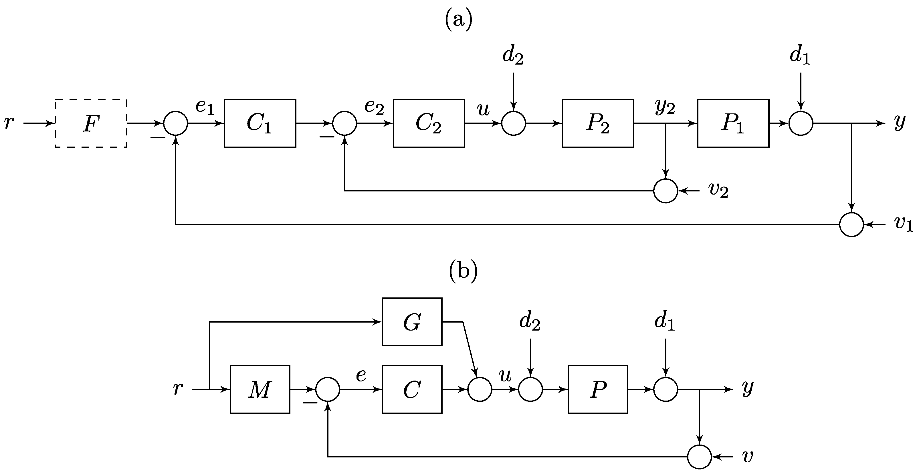
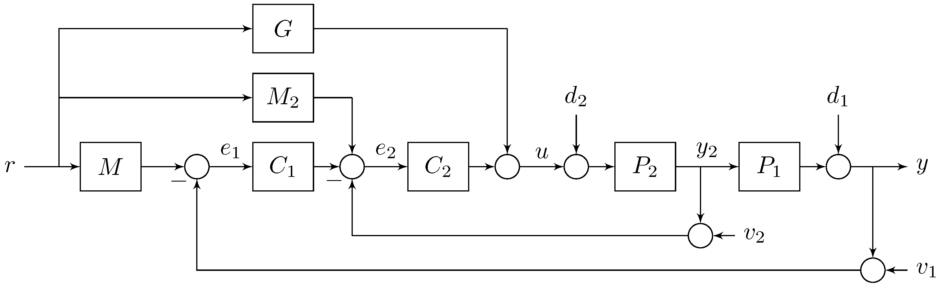
2.1. Control Structure

Figure 2 shows the proposed architecture. Transfer-function models and signals in the block diagram can be described as follows. The inner measurement $y_2$ divides the plant from the single control input u to the controlled output y into two plant models: the outer $P_1$ and the inner $P_2$ ones. Outer y and inner $y_2$ measurements are contaminated with high frequency-band noise of zero mean, $v_1$ and $v_2$, respectively. External disturbances $d_1$ and $d_2$ can be also incorporated in the system. The model M expresses the desired behavior of the controlled output y for the tracking of the reference r; deviations between $rM$ and y are detected in the feedback error signal $e_1$ to be corrected. Similarly, $M_2$ is the r tracking model for $y_2$, and $e_2$ detects the mismatches. The elements object of design are the two feedback controllers, $C_1$ and $C_2$, and the feedforward controller, G. The use of a single feedforward controller G will impose some restrictions to solve the robust control problem under QFT paradigm. In particular, the tracking model for $y_2$ must be defined in close relation to the tracking model for $y=y_1$ as follows:

$$M_2=M/P_1,$$

(1)

under the assumption that $P_1$ is a fixed transfer function, i.e., no uncertainty can be defined for this plant model. This corresponds to reality when $P_1$ is a pure integrator, and the output and its derivative can be measured for feedback; position and speed are illustrative examples in motion systems [9,22,23]. M should be also cautiously chosen to obtain a strictly proper transfer function in (1).

According to the control scheme, the controlled output depends on the external inputs as follows:

$$\begin{array}{c}\hfill y=\frac{(M{C}_1{C}_2+M_2{C}_2+G)P_1{P}_2}{1+L_t}r+\frac{(1+L_2)}{1+L_t}{d}_1+\frac{P_1{P}_2}{1+L_t}{d}_2-\frac{L_1}{1+L_t}{v}_1-\frac{L_t/C_1}{1+L_t}{v}_2,\end{array}$$

(2)

where $L_t$ is the total open-loop transfer function

$$L_t=L_1+L_2,$$

(3)

which is contributed by the open-loop transfer functions of the outer loop

$$L_1=C_1{C}_2{P}_1{P}_2$$

(4)

and the inner loop

$$L_2=C_2{P}_2.$$

(5)

The tracking error $e=e_1$ can be obtained by computing $Mr-y$, which after substituting y of (2) and some simplifications yields

$$e=\frac{M-G{P}_1{P}_2}{1+L_t}r-\frac{(1+L_2)}{1+L_t}{d}_1-\frac{P_1{P}_2}{1+L_t}{d}_2-\frac{(1+L_2)}{1+L_t}{v}_1-\frac{C_2{P}_1{P}_2}{1+L_t}{v}_2.$$

(6)

Some intermediate results to obtain the first term of (6) are

$$\begin{array}{cc}{e}_r=Mr-y_r\hfill & =Mr-\frac{(M{C}_1{C}_2+M_2{C}_2+G)P_1{P}_2}{1+L_1+L_2}r\hfill \\ & \hfill =\frac{M+M{L}_1+M{L}_2-M{L}_1-M_2{C}_2{P}_1{P}_2-G{P}_1{P}_2}{1+L_1+L_2}r=\frac{M-G{P}_1{P}_2}{1+L_1+L_2}r,\end{array}$$

(7)

considering

$$M_2{C}_2{P}_1{P}_2=M{P}_1^{-1}{C}_2{P}_1{P}_2=M{C}_2{P}_2=M{L}_2.$$

(8)

The control action, expressed as a function of the external inputs, is

$$u=\frac{(M{C}_1{C}_2+M_2{C}_2+G)}{1+L_t}r-\frac{C_1{C}_2}{1+L_t}{d}_1-\frac{L_t}{1+L_t}{d}_2-\frac{C_1{C}_2}{1+L_t}{v}_1-\frac{C_2}{1+L_t}{v}_2.$$

(9)

2.2. Robust Control under QFT Paradigm

Robust reference tracking, robust disturbance rejection, and robust stability mean that those control specifications are met by any plant in the uncertain set defined. For the present study, let us define the vector

$$\mathrm{q}=[q_1,q_2,q_3,\cdots ,q_w],$$

(10)

which contains the w parameters used to define the parametric uncertainty of model $P_2$. The value of each parameter $q_i\in \mathrm{q}$ can vary in-between a lower $q_i^{-}$ and an upper $q_i^{+}$ limit. Hence the uncertainty vector q belongs to an hyper-rectangle in ${\mathbb{R}}^w$ called the uncertainty space $\mathcal{Q}$, i.e.,

$$\mathrm{q}\in \mathcal{Q}\triangleq \{\mathrm{q}\in {\mathbb{R}}^w|q_i^{-}\le q_i\le q_i^{+},i=1,\cdots ,w\},$$

(11)

which yields a set of inner plant models

$${\mathcal{P}}_2=\{P_2(s;\mathrm{q}):\mathrm{q}\in \mathcal{Q}\}.$$

(12)

Let us remember that no uncertainty is possible for $P_1$, and the most common case will be adopted hereinafter for the outer plant:

$$P_1=\frac{1}{s}.$$

(13)

QFT is a frequency domain method. The frequency response ($s=j\omega$) of a discrete set of plants in ${\mathcal{P}}_2$ together with the frequency response of $P_1$ will be handled. Robust control specifications will be formulated as inequalities that constrain the magnitude frequency response of closed-loop transfer functions.

Robust stability requirements affect both feedback loops, which is formulated as

$$\left|\frac{C_1\left(j\omega \right)C_2\left(j\omega \right)P_1\left(j\omega \right)P_2\left(j\omega \right)}{1+C_2\left(j\omega \right)P_2\left(j\omega \right)+C_1\left(j\omega \right)C_2\left(j\omega \right)P_1\left(j\omega \right)P_2\left(j\omega \right)}\right|\le B_{s_1}\left(\omega \right);\forall P_2\in {\mathcal{P}}_2$$

(14)

and

$$\left|\frac{C_2\left(j\omega \right)P_2\left(j\omega \right)}{1+C_2\left(j\omega \right)P_2\left(j\omega \right)}\right|\le B_{s_2}\left(\omega \right);\forall P_2\in {\mathcal{P}}_2,$$

(15)

where $B_{s_1}\left(\omega \right)$ and $B_{s_2}\left(\omega \right)$ are upper tolerances for the complementary sensitivity function of their respective feedback loops. These tolerances are related with the desired stability margins [24]; includes some arguments about it. At designer’s discretion, take

$$B_{s_{i=1,2}}=\frac{1}{2sin(\mathrm{PM}/2)},$$

(16)

if the phase margin (PM) is chosen, or

$$B_{s_{i=1,2}}=\frac{\mathrm{GM}}{\mathrm{GM}-1},$$

(17)

if the gain margin (GM) is preferred.

Robust disturbance rejection can be considered by

$$\left|\frac{e\left(j\omega \right)}{d_2\left(j\omega \right)}\right|=\left|\frac{-P_1\left(j\omega \right)P_2\left(j\omega \right)}{1+C_2\left(j\omega \right)P_2\left(j\omega \right)+C_1\left(j\omega \right)C_2\left(j\omega \right)P_1\left(j\omega \right)P_2\left(j\omega \right)}\right|\le B_{d_2}\left(\omega \right);\forall P_2\in {\mathcal{P}}_2$$

(18)

for disturbances at the plant input, and by

$$\left|\frac{e\left(j\omega \right)}{d_1\left(j\omega \right)}\right|=\left|\frac{-(1+C_2\left(j\omega \right)P_2\left(j\omega \right))}{1+C_2\left(j\omega \right)P_2\left(j\omega \right)+C_1\left(j\omega \right)C_2\left(j\omega \right)P_1\left(j\omega \right)P_2\left(j\omega \right)}\right|\le B_{d_1}\left(\omega \right);\forall P_2\in {\mathcal{P}}_2$$

(19)

for disturbances at the plant output. Upper tolerances $B_{d_1}$ and $B_{d_2}$ can be selected as in any other QFT problem [1,25]. As long as the novelty of the new structure is for reference tracking, disturbance rejection specifications play a secondary role hereinafter.

Robust reference tracking constrains the tracking error as

$$\begin{array}{cc}\left|\frac{e\left(j\omega \right)}{r\left(j\omega \right)}\right|=\hfill & \left|\frac{M\left(j\omega \right)-G\left(j\omega \right)P_1\left(j\omega \right)P_2\left(j\omega \right)}{1+L_t\left(j\omega \right)}\right|=\hfill \\ & \hfill \left|\frac{M\left(j\omega \right)-G\left(j\omega \right)P_1\left(j\omega \right)P_2\left(j\omega \right)}{1+C_2\left(j\omega \right)P_2\left(j\omega \right)+C_1\left(j\omega \right)C_2\left(j\omega \right)P_1\left(j\omega \right)P_2\left(j\omega \right)}\right|\le B_r\left(\omega \right);\forall P_2\in {\mathcal{P}}_2\end{array}$$

(20)

The selection of the upper tracking tolerance $B_r$ follows the criteria of error-tracking or model-matching works, as per example [1,15].

The design of G must be separated from the design of $C_1$ y $C_2$ as follows. In a similar fashion to [15], Equation (20) is rewritten as

$$\left|\frac{-M\left(j\omega \right)}{P_1\left(j\omega \right)P_2\left(j\omega \right)}+G\left(j\omega \right)\right|\le B_r\left(\omega \right)\left|\frac{1+L_t\left(j\omega \right)}{P_1\left(j\omega \right)P_2\left(j\omega \right)}\right|;\forall P_2\in {\mathcal{P}}_2,$$

(21)

which reveals as valid G those inside the region delimited by a circumference of center

$$\frac{-M\left(j\omega \right)}{P_1\left(j\omega \right)P_2\left(j\omega \right)},$$

(22)

and radii

$$B_r\left(\omega \right)\left|\frac{1+L_t\left(j\omega \right)}{P_1\left(j\omega \right)P_2\left(j\omega \right)}\right|$$

(23)

in the complex plane. For a discrete $\omega$ frequency, each plant within a discrete set ${\mathcal{P}}_2$ defines its own circumference. Then two plant cases $P_{2_u},P_{2_v}\in {\mathcal{P}}_2$ share a common solution G if the distance between the centers of circumferences is equal to or shorter than the sum of their radii. This condition responds to

$$\begin{array}{cc}\left|\frac{M\left(j\omega \right)}{P_1\left(j\omega \right)P_{2_u}\left(j\omega \right)}-\frac{M\left(j\omega \right)}{P_1\left(j\omega \right)P_{2_v}\left(j\omega \right)}\right|\hfill & \le \hfill \\ & \hfill B_r\left(\omega \right)\left|\frac{1+L_{t_u}\left(j\omega \right)}{P_1\left(j\omega \right)P_{2_u}\left(j\omega \right)}\right|+B_r\left(\omega \right)\left|\frac{1+L_{t_v}\left(j\omega \right)}{P_1\left(j\omega \right)P_{2_v}\left(j\omega \right)}\right|,\end{array}$$

(24)

which evidences the mission of the feedback controllers $C_1$ and $C_2$ in $L_t$. These must enlarge the circumference radii (23) sufficiently such that any plant pair in the uncertainty set, $\forall P_{2_u},P_{2_v}\in {\mathcal{P}}_2$, met (24), which in turn ensures the existence of G. Hence, to achieve (20), $C_1$ and $C_2$ are firstly designed for (24), and then G to finally satisfy (21).

Let us notice that (24) expresses the strictly minimum amount of feedback $L_t$ that is necessary, and this would be the same whatever the number of nested loops; global feedback $L_t$ only depends on the global plant $P_1{P}_2$ and the specification $M,Br$. That unique $L_t$ is contributed by $L_t=C{P}_1{P}_2$ for single feedback (Figure 1b) and by $L_t=C_1{C}_2{P}_1{P}_2+C_2{P}_2$ for double feedback (Figure 2), which reveals $C_1{C}_2<C$. Then, a relevant benefit of double feedback is reducing the individual controller bandwidth, which mainly reduces the sensor noise amplification at u. For single feedback, the v noise transmission is $u=-C/(1+L_t)v$, whereas for double feedback how the two noise sources $v_1,v_2$ are transmitted to u (9) can be shaped and the $v_1=v$ noise transmission $u=-C_1{C}_2/(1+L_t)v_1$ is definitely reduced in comparison to single feedback.

To quantify the global influence of all noise sources, let us define the Root Mean Squared value $V_t$ of total noise at u such that

$$V_t^2=V_{t_1}^2+V_{t_2}^2={\int }_0^{\infty }{\left|\frac{C_1\left(j\omega \right)C_2\left(j\omega \right)}{1+L_t\left(j\omega \right)}\right|}^2{\Phi }_1\left(\omega \right)d\omega +{\int }_0^{\infty }{\left|\frac{C_2\left(j\omega \right)}{1+L_t\left(j\omega \right)}\right|}^2{\Phi }_2\left(\omega \right)d\omega ,$$

(25)

where ${\Phi }_{i=1,2}$ is the power spectral density of noise source $v_{i=1,2}$ (sensors are modeled as white noise sources, i.e., ${\Phi }_i\left(\omega \right)$ takes a constant value over the frequency band), and $V_{t_i}^2$ represents a mean-squared value that measures the individual contribution. Then, $L_t$ can be conveniently allocated between $L_1=C_1{C}_2{P}_1{P}_2$ and $L_2=C_2{P}_2$ to reduce as much as possible the gain of feedback controllers over the frequency band: $|C_1\left(j\omega \right)C_2\left(j\omega \right)|$ on the one side and $|C_2\left(j\omega \right)|$ on the other side. In this case, the branches $L_1$ and $L_2$ are not independent since $C_2$ contributes to both, similarly to what happened in the serial structure of controllers for MISO systems [20]. A similar procedure to [19,20] will be followed to allocate the bandwidth. Thus, the new method firstly analyzes the two extreme cases in which only one of the two loops provides the $L_t$ that is fixed by (24). If only $L_2$ works ($C_1=0$), the needed controller becomes $C_2\left(j\omega \right)=L_t\left(j\omega \right)/P_2\left(j\omega \right)$. On the other hand, if only $L_1$ works (the inner loop is opened), the needed controller becomes $C_1\left(j\omega \right)C_2\left(j\omega \right)=L_t\left(j\omega \right)/\left(P_1\left(j\omega \right)P_2\left(j\omega \right)\right)$. Therefore, since $L_t$ is fixed, the magnitude frequency response of controllers will depend on the magnitude frequency response of the plants. The higher the plant magnitude, the lower the controller gain. In the present case, $P_1$ is an integrator, $|P_1\left(j\omega \right)P_2\left(j\omega \right)|$ is higher than $|P_2\left(j\omega \right)|$ over low frequencies, and the other way round happens over high frequencies. The switching frequency is $\omega =1$ from $|P_1\left(j\omega \right)P_2\left(j\omega \right)|=|P_2\left(j\omega \right)|$ and $P_1\left(j\omega \right)=j{\omega }^{-1}$. Consequently, $L_1$ should work over $\omega \le 1$ and $L_2$ over $\omega \ge 1$ to obtain the minimum possible gain of $C_1{C}_2$ and $C_2$ over the whole frequency band; the working band of one loop must be understood as the frequencies where this loop contributes with a higher gain than the other.

For any other plant $P_1$ different from an integrator, a comparison between $|P_1\left(j\omega \right)P_2\left(j\omega \right)|$ and $|P_2\left(j\omega \right)|$ should be done. Thus, $L_1$ should work over the frequencies where $|P_1\left(j\omega \right)|\le 1$, and $L_2$ over the frequencies where $|P_1\left(j\omega \right)|\ge 1$.

The previous strategy minimizes $V_t$ (25) under the assumption that the noise sources $v_1$ and $v_2$ are equal, which is probably not a real case. If ${\Phi }_1<{\Phi }_2$, the working band of $L_1$ should be widened with respect to the previous criterion, whereas ${\Phi }_1>{\Phi }_2$ should widen the working band of $L_2$. In summary, any $L_t$ load-sharing between $L_1$ and $L_2$ can be established. Once the working bands are chosen, a method for designing the controllers that satisfy them is indicated below.

3. Design Methodology

As usual in QFT, feedback controllers $C_1$ and $C_2$ are designed first, and then the feedforward controller G. Feedback $C_1$ and $C_2$ are in charge of achieving robust stability specifications (14) and (15), robust disturbance specifications (18), and (19) if they exist, and the part of the robust reference tracking (20) that attains feedback, i.e., (24). Later, the design of the feedforward G at a second stage must meet (21), which finally implies that the set $C_1$, $C_2$, and G achieves (20).

The designs are performed in the frequency domain by shaping certain functions of $\omega$ that must meet bounds at a discrete set of frequencies

$$\Omega =[{\omega }_1,{\omega }_2,{\omega }_3,\cdots {\omega }_z].$$

(26)

The bounds that guide the loop-shaping are depicted on the complex plane (phase, logarithmic magnitude).

For feedback designs, the bounds represent the closed-loop specifications in terms of a nominal open-loop transfer function, $L_{1_0}\left(j\omega \right)$, or $L_{2_0}\left(j\omega \right)$, in such a way that if $L_{i_0}\left(j\omega \right)$ satisfies its bound set for the nominal plant case, the whole set of plants will satisfy it. Previously, plant templates were computed. They represented the frequency response of a discrete set of plants plants in ${\mathcal{P}}_2$ (12) multiplied by plant $P_1$ (13); any plant in the template could be chosen as the nominal case $P_{1_0}{P}_{2_0}$. Templates and bounds could be computed with standard CAD tools whenever the specifications followed standard formulas (the terminology in the original works has been adapted to the current nomenclature). In particular, tracking specifications with feedback C and feedforward G must respond to the general format [16]

$$\left|\frac{A+BG}{D+EC}\right|\le W,$$

(27)

and specifications with solely feedback C must follow the format [11]

$$\left|\frac{A+BC}{D+EC}\right|\le W.$$

(28)

In these equations, G and C denote the feedforward and feedback controllers, respectively; W is the upper tolerance for the magnitude of the closed-loop frequency response; and A, B, D and E are expressions that include known functions such as the plants $P_1$ and $P_2$, the models M and $M_2$, or the feedback controller that is taken as fixed when the other feedback controller is going to be designed. The work [16] developed how to separately obtain the bounds for feedback and feedforward from (27), and how to integrate them in the CAD tool [11]; a procedure similar to the one in Section 2.2 and [15] was followed. Specifications of the form (28) were handled with the original function genbnds of the toolbox [11].

There are infinity couples, $C_1\left(j\omega \right),C_2\left(j\omega \right)$, which achieve the control specifications. The targets are those that allocate the control bandwidth between $L_1$ and $L_2$ as per predefined. There is a single pair of feedback controllers that reduces as much as possible the sensor noise amplification $V_t$ (25). A sequential procedure is proposed in the following to shape firstly $L_{2_0}\left(j\omega \right)$, which is in charge of the high frequencies, and secondly $L_{1_0}\left(j\omega \right)$, which is in charge of the low frequencies; Section 2.2 proposed guidelines to choose the switching frequency between both loops. Step-by-step procedures of loop-shaping to allocate the control bandwidth between loops are given in [19,20]. Once $C_1$ and $C_2$ are designed, some guidelines on the design of G will be given for the full achievement of tracking specification.

3.1. First Stage: Design of the Inner Feedback Controller

The controllers are initially set to zero, $C_1=C_2=0$; in the case of returning back to this step, the controllers could take non null values. The sequence begins with the design of $C_2$ by shaping $L_{2_o}\left(j\omega \right)=C_2\left(j\omega \right)P_{2_o}\left(j\omega \right)$; this inner loop will be in charge of the mid-high frequencies inside the control bandwidth. Bounds for $L_2$ loop are computed as follows considering that $C_2$ is the unknown.

Comparing (15) with the standard (28), the $L_2$-bounds for inner loop stability can be computed by choosing $A=0$, $B=P_2$, $D=1$, $E=P_2$, $C=C_2$ and $W=B_{s_2}$ in (28).

Comparing (14) with the standard (28), the $L_2$-bounds for outer loop stability can be computed by choosing $A=0$, $B=C_1{P}_1{P}_2$, $D=1$, $E=P_2+P_2{P}_1{C}_1$, $C=C_2$ and $W=B_{s_1}$ in (28).

Comparing (20) with the standard (27), the G-bounds and the $L_2$-bounds for tracking can be independently computed by choosing $A=M$, $B=-P_1{P}_2$, $G=G$, $D=1$, $E=P_2+P_2{P}_1{C}_1$, $C=C_2$ and $W=B_r$ in (27). At the current step, only the $L_2$-bounds are being considered.

In a similar fashion, the $L_2$-bounds for disturbance rejection problems can be obtained comparing (18) and (19) with the standard (28). For the sake of clarity, no disturbance rejection specifications are being considered hereinafter.

Once the whole set of bounds is found, the less favorable set is computed by intersecting the bounds that represent the specifications at each frequency. A single bound prevails at each discrete frequency: ${\beta }_{L_2}\left(\omega \right)$, $\omega \in \Omega$ (26). Subsequently, $L_{2_o}\left(j\omega \right)$ is shaped to only meet the bounds ${\beta }_{L_2}\left(\omega \right)$ at frequencies in $\Omega$ above the switching frequency between loops $L_1$ and $L_2$. Therefore, $L_{2_o}\left(j\omega \right)$ momentarily violates the bounds at the working frequencies of the other loop. The $L_2$-shaping yields $C_2$.

3.2. Second Stage: Design of the Outer Feedback Controller

This outer loop will be in charge of the low frequencies (up to the switching frequency). Bounds for $L_1$ loop are computed as follows considering that $C_1$ is the unknown; let us take for $C_2$ the controller that was obtained in the previous step.

Comparing (14) with the standard (28), the $L_1$-bounds for outer loop stability can be computed by choosing $A=0$, $B=C_2{P}_2{P}_1$, $D=1+C_2{P}_2$, $E=C_2{P}_2{P}_1$, $C=C_1$ and $W=B_{s_1}$ in (28).

Comparing (20) with the standard (27), the G-bounds and the $L_1$-bounds for tracking can be independently computed by choosing $A=M$, $B=-P_1{P}_2$, $G=G$, $D=1+C_2{P}_2$, $E=C_2{P}_2{P}_1$, $C=C_1$ and $W=B_r$ in (27). In the present step, only the $L_1$ bounds are being taking into account.

In a similar fashion, the $L_1$-bounds for disturbance rejection can be obtained comparing (18) and (19) with the standard (28). For the sake of clarity, no disturbance rejection specifications are being considered hereinafter.

The intersection of the whole set of previous bounds at each discrete frequency (26) yields ${\beta }_{L_1}\left(\omega \right)$, $\omega \in \Omega$. Subsequently, $L_{1_o}\left(j\omega \right)$ is shaped to meet the bounds ${\beta }_{L_1}\left(\omega \right)$ at the whole set of frequencies $\Omega$ (26). At this design step, $L_2$ has already provided the necessary feedback for tracking at frequencies above the inter-loop switching frequency, and consequently the bounds ${\beta }_{L_1}\left(\omega \right)$ take on a circular shape at these frequencies to preserve the necessary stability margins. The switching frequency between loops can be taken as a roll-off frequency for $L_1$ in such a way that it is advisable to reduce the $L_{1_o}\left(j\omega \right)$ gain as fast as possible from this frequency ahead. The $L_1$-shaping yields $C_1$.

Once $C_1$ is designed, the $L_2$-bounds are updated. As a result the new disposition of ${\beta }_{L_2}\left(\omega \right)$ must evidence that $L_{2_o}\left(j\omega \right)$ now satisfies them at the whole set of design frequencies $\Omega$ (26). A new iteration (coming back to the first stage) is recommended if this does not happen or over-design is detected (more $L_{2_o}$ gain than ${\beta }_{L_2}$ demands at certain $\omega$). Then, $L_{2_o}\left(j\omega \right)$ and $L_{1_o}\left(j\omega \right)$ can be sequentially re-shaped, which yields new feedback controllers; these will be used as initial values to recompute the bounds on the other loop. Let us recall that the final objective of double feedback was reducing as much as possible the controller gains to minimize $V_t$ (25). Thus, it is recommended that $L_{2_o}\left(j\omega \right)$ and $L_{1_o}\left(j\omega \right)$ finally lie on their respective bounds, ${\beta }_{L_2}\left(\omega \right)$ and ${\beta }_{L_1}\left(\omega \right)$, or as close as possible to them.

For a different switching frequency between loops, there would be another pair of $L_{2_o}\left(j\omega \right)$, $L_{1_o}\left(j\omega \right)$ that exactly lie on their bounds, i.e., that satisfy the performance and stability specifications. Then, it is convenient to compute $V_t$ (25) in such a way that the switching frequency between loops may be altered at any moment in the design sequence to reduce $V_t$.

3.3. Third Stage: Design of the Feedforward Controller

Let us take the feedback controllers $C_1$ and $C_2$ that were computed after the previous steps. The unknown is now the feedforward element G, which must complete the fulfillment of the tracking specification (20). Comparing it with the standard (28), the G-bounds can be computed by choosing $A=M$, $B=-P_1{P}_2$, $D=1+P_2{C}_2+P_1{P}_2{C}_1{C}_2$, $E=0$, and $C=G$ in (28).

Let us denote the G-bounds as ${\beta }_G\left(\omega \right)$. At each discrete frequency $\omega \in \Omega$ (26), ${\beta }_G\left(\omega \right)$ delimits a closed region in the complex plane, which contains possible solutions for $G\left(j\omega \right)$. Those regions enlarge with the over-design of feedback controllers; over-design happens when controllers have more gain than the strictly necessary to satisfy the specifications or, in other words, when $L_{i_o}\left(j\omega \right)$ does not exactly lie on ${\beta }_{L_i}\left(\omega \right)$ bounds. Some feedback over-design is recommended to ease the shaping of $G\left(j\omega \right)$ or to reduce the order of $G\left(s\right)$. The price paid is that $V_t$ (25) increases.

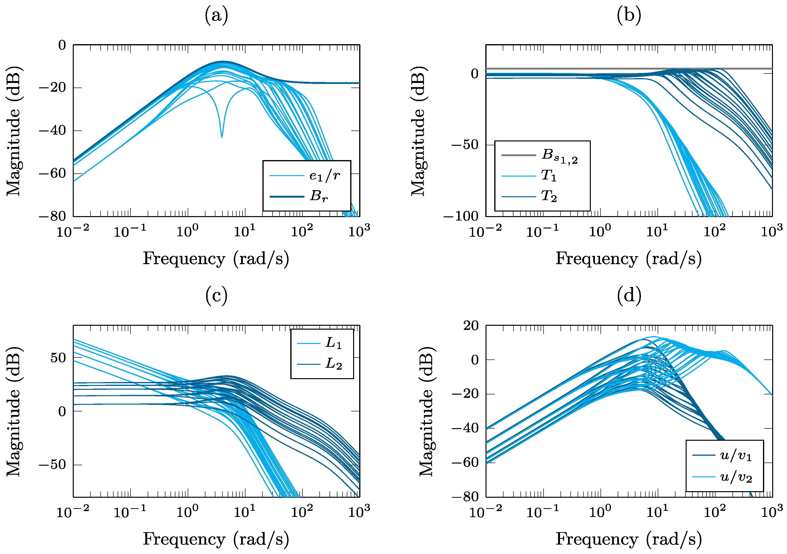
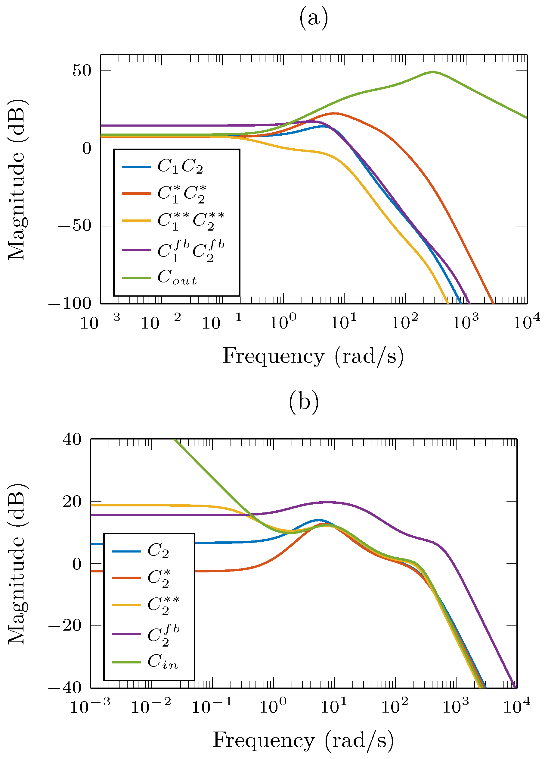
4. Design Example and Comparisons

The following robust control problem is proposed. The plants are

$$P_2\left(s\right)=\frac{k\times a}{(s+a)},k\in \left[110\right],a\in \left[110\right];P_1\left(s\right)=\frac{1}{s}.$$

(29)

The tracking specification (20) considers the model

$$M\left(s\right)=\frac{{\omega }_n^2}{(s^2+2\delta {\omega }_{n}s+{\omega }_n^2)}=\frac{32.65}{(s^2+8s+32.65)},$$

(30)

and the upper tolerance for the magnitude frequency response of error

$$B_r\left(\omega \right)={\left|\frac{0.2s(s/25+1)}{{(s/4+1)}^2}\right|}_{s=j\omega }.$$

(31)

A phase margin of at least ${40}^{\circ }$ is desired for robust stability of the outer and inner loops. Taking $\mathrm{PM}=40$ in (16), the upper tolerances for the magnitude frequency response of complementary sensitivity functions (14) and (15) became

$$B_{s_1}\left(\omega \right)=B_{s_2}\left(\omega \right)=1.46.$$

(32)

For the sake of clarity, no disturbance specifications will be considered. In addition, identical power spectral ${\Phi }_1={\Phi }_2$ of the noises from both sensors $v_1$ and $v_2$ will be assumed. The set of discrete frequencies is

$$\Omega =[0.1,0.3,0.6,1,3,6,10,100].$$

(33)

Firstly, the said robust control problem will be solved to illustrate the new design methodology and the benefits of the new control structure. A second subsection will establish some comparisons to highlight the novelties of the proposal. The new structure [Figure 2] will be compared with the two control architectures that were feasible to date in robust QFT control [Figure 1, cascading and model-matching structures]; this will reveal the utility of the new degrees of freedom. For the new control structure, two other robust QFT control solutions will be given that allocate the feedback control bandwidth differently between both loops; this will validate the proposed method to choose the best switching frequency between loops. In all the comparisons, let us remember that the final objective is to reduce as much as possible the amplification of sensor noises $v_1$ and $v_2$ at the actuation u. Equation (9) revealed that this was closely related to the magnitude frequency response of feedback controllers in the outer loop ($C_1{C}_2$) and the inner loop ($C_2$). In addition, Equation (25) computed an accumulative impact of this noise transmission along the frequency; $V_{t_1}^2$ and $V_{t_2}^2$ measured the total impact of each source, which were added to give $V_t^2$. Then, to compare all solutions mentioned, a figure will show the magnitude frequency response of feedback controllers and a table will collect the noise impacts. To compute (25), the noise sources will be simulated as Band-Limited White Noise of power amplitude = $0.0001$, sample time = $0.001$ s; integrals will be approximated by a discrete integration over the frequency range $\omega \in [{10}^{-2},{10}^3]$.

4.1. Solution Achieved by the New Proposal

As Section 3 indicated, $L_1\left(j\omega \right)$ should work over $\omega \le 1$ and $L_2\left(j\omega \right)$ should work over $\omega \ge 1$, and accordingly a design method of three main steps was proposed. For the current robust control problem (29)–(33), it yields the feedback controllers

$$C_2\left(s\right)=\frac{93451(s+40)(s+1.56)(s+0.018)}{(s+0.019)(s^2+9.462s+32.49)(s^2+535.7s+8.294\times {10}^4)},$$

(34)

$$C_1\left(s\right)=\frac{53.9}{(s^2+9.8s+49)},$$

(35)

and the feedforward controller

$$G\left(s\right)=\frac{722.35s(s+1.2)(s^2+16.32s+277.2)}{(s+86)(s^2+6.702s+24.5)(s^2+14.98s+207.4)}.$$

(36)

Figure 3 depicts how the bounds ${\beta }_{L_1}\left(\omega \right)$, ${\beta }_{L_2}\left(\omega \right)$ and ${\beta }_G\left(\omega \right)$ are finally met by shaping of $L_{1_o}\left(j\omega \right)$, $L_{2_o}\left(j\omega \right)$ and $G\left(j\omega \right)$, respectively.

Figure 4 validates the designs by showing those frequency responses of interest (magnitude Bode diagrams are used). Fourteen plant cases were considered for (29). Figure 4a shows the fulfillment of the robust tracking-error specification; let us note as the upper tolerance $B_r$ is tightly met up to $\omega \approx 40$ rad/s. Figure 4b shows the fulfillment of robust stability; inner $T_2$ and outer $T_1$ complementary sensitivity functions are depicted. Figure 4c shows the prescribed frequency allocation of $L_t$ between both loops with a switching frequency around $\omega =1$. Figure 4d shows the implicit target about the transmission of sensor noises $v_1$ and $v_2$ to the plant input u; it is depicted the magnitude frequency response of the transmission functions $|C_1{C}_2/(1+L_t)|$ and $|C_2/(1+L_t)|$. These reveal how noise amplifications happen from the switching frequency $\omega =1$ up to around the gain cross-over frequency of each $L_i$, i.e., up to $\omega =20$ for $L_1$ and up to $\omega =200$ for $L_2$. Obviously, the noise amplification of the inner sensor is larger since $L_2$ has a higher gain cross-over frequency than $L_1$. Plot (d) will gain meaning in the comparisons with other solutions. In a quantitative manner, the accumulative noise transmission at the control input (25) yields $V_t=0.3429$, and the individual squared contributions of each sensor are $V_{t_1}^2=0.01$ and $V_{t_2}^2=0.1076$.

Figure 5 shows the time-domain behavior of fourteen plant cases. It considers the following external inputs: the reference $r\left(t\right)$ suffers a unity step change at $t=1$ s, and the sensor noises $v_1\left(t\right)$ and $v_2\left(t\right)$ are built with Band-Limited White Noise sources (power amplitude = $0.0001$, sample time = $0.001$ s). Figure 5a shows how the closed-loop responses $y\left(t\right)$ are conveniently distributed up and down the desired response $m\left(t\right)$, which corresponds to the model M (30). Let us recall that the contained dispersion obeys to the tolerance $B_r$ (31). There are also depicted the control efforts [Figure 5b,c]: the control action to the actuator $u\left(t\right)$ is built by the sum of feedback $u_c\left(t\right)$ and feedforward $u_g\left(t\right)$ actions. It could be assimilated $u_g\left(t\right)$ to the control effort that is needed to produce $m\left(t\right)$ whereas $u_c\left(t\right)$ compensates output deviations due to the plant uncertainty. Sensor noises hardly affect the output while they are noticeable at the control input; a moderate impact has been achieved thanks to an adequate distribution of the amount of feedback between both loops.

4.2. Comparatives with Other Structures and Strategies

Another solution to the robust control problem (29)–(33) is given below using a model-matching structure of single feedback [see Figure 1b]. It yields a feedback controller

$$C_{out}\left(s\right)=\frac{92434(s+68.74)(s+0.5971)}{(s+16.87)(s^2+346.2s+8.325\times {10}^4)}$$

(37)

and a feedforward controller

$$G_{out}\left(s\right)=\frac{556.16s(s+1.293)(s+2.206)(s+24.87)}{(s+10.29)(s+2.792)(s+68.04)(s^2+9.704s+35.35)}.$$

(38)

Figure 6a shows how the solution of outer single feedback implies a considerably large bandwidth of controller $C_{out}$ since it has been forced to work in the high frequency band where $P_1{P}_2$ presents very small magnitude in comparison with $P_2$. In addition, since $L_t$ is the same as in double feedback ($C_1{C}_2$), the magnitude frequency response $|u/v_1|$ will have a much larger peak than in Figure 4d. Finally, this means a huge amplification of the single sensor noise at the actuator. It results in a RMS value (25) of $V_t=78.0065$, this being much higher than for the new architecture that employs double feedback [see rows 1 and 2 of

Table 1. Effective values of sensor noise transmissions at the actuator (25).

Design Strategy	Degrees of Freedom			${\mathit{V}}_{\mathit{t}}$	${\mathit{V}}_{{\mathit{t}}_1}^2$	${\mathit{V}}_{{\mathit{t}}_2}^2$
New architecture; ${\omega }_{sw}=1$	G (36)	$C_1$ (35)	$C_2$ (34)	0.3429	0.001	0.1076
Model matching; outer feedback	$G_{out}$ (38)	$C_{out}$ (37)	——	78.0065	6085	0
Model matching; inner feedback	$G_{in}$ (40)	—-	$C_{in}$ (39)	0.3780	0	0.1429
Double feedback; no feedforward	—–	$C_1^{fb}$ (42)	$C_2^{fb}$ (43)	1.1882	0.0053	1.4065
New architecture; ${\omega }_{sw}=5$	$G^{*}$ (46)	$C_1^{*}$ (44)	$C_2^{*}$ (45)	0.6929	0.3797	0.1004
New architecture; ${\omega }_{sw}=0.5$	$G^{**}$ (49)	$C_1^{**}$ (47)	$C_2^{**}$ (48)	0.3586	0.00022	0.1284

]. This situation would spoil the expected performance in real life, which if this noise did not exist would coincide with $y\left(t\right)$ in Figure 5a. This fact highlights the usefulness of cascade feedback loops when inner state measurements are available.

* * *

The control structure of previous solution [Figure 1b] is equivalent to cut off the feedback and feedforward connections to $e_2$ sum point in the new control architecture [Figure 2]. Similarly to only using the outer loop, let us consider as another theoretically possible solution the use of only the inner loop, i.e., feedback and feedforward connections to $e_1$ sum point are cut off. This control architecture would be viable for tracking since $P_1\left(s\right)$ has no uncertainty, but the constant presence of disturbances makes the feedback of output necessary in practice. Nevertheless, the solution will help to understand how the load-sharing between loops affects the noise amplification. To solve the robust control problem (29)–(33), the said structure employs the feedback controller

$$C_{in}\left(s\right)=\frac{70976(s+56)(s+2.9)(s+1)}{s(s^2+15.3s+72.25)(s^2+322.4s+6.76\times {10}^4)},$$

(39)

and the feedforward controller

$$G_{in}\left(s\right)=\frac{739.14s(s+1.2)}{(s+70)(s^2+6.72s+23.04)}.$$

(40)

Figure 6b shows how the solution of inner single feedback implies a considerably larger gain of $C_{in}$ at low frequencies since the inner loop has been forced to work at low frequencies without the help of the outer controller. However, $|1+L_t|$ also reaches high values over these frequencies, which constrains $|C_{in}/(1+L_2)|$. Therefore, it is around the cross-over frequency of $L_t=L_2$ where the excess of feedback gain affects the noise amplification. Finally, the inner single feedback results in an RMS value of $V_t=0.3780$; it is entirely contributed by $V_{t_2}^2=0.1429$, which results slightly higher than that of the new architecture with double feedback [compare rows 1 and 3 of Table 1]. However, let us remark that the weak point of this architecture is the impossibility of rejecting disturbances outside the internal feedback loop, i.e., the output is in open loop.

* * *

Until the present work, there was no formal method for the design of double-feedback plus feedforward within the QFT paradigm. In fact, the architecture of Figure 1a, which lacks of feedforward loops, was used for robust disturbance rejection problems. Now, the architecture of Figure 2 with $G=0$ will be used to solve the robust tracking problem (29)–(33). Let us note that feedforward loops with known information (M and $M_2$) remain for a fair comparison with the new structure, i.e., the only difference is the lack of tunable feedforward. Then, Equation (20) turns into

$$\begin{array}{c}\hfill \left|\frac{e\left(j\omega \right)}{r\left(j\omega \right)}\right|=\left|\frac{M\left(j\omega \right)}{1+C_2\left(j\omega \right)P_2\left(j\omega \right)+C_1\left(j\omega \right)C_2\left(j\omega \right)P_1\left(j\omega \right)P_2\left(j\omega \right)}\right|\le B_r\left(\omega \right);\forall P_2\in {\mathcal{P}}_2,\end{array}$$

(41)

which corresponds to the format (28). Then, $L_i$-bounds can be computed by using the classical function genbnds of the Terasoft toolbox [11]. The same frequency band assignment will be made for $L_1$ and $L_2$ as in the first solution (switching frequency at $\omega =1$). The same design method yields the feedback controllers

$$C_1^{fb}=\frac{19.66}{(s^2+6.58s+22.09)}$$

(42)

and

$$C_2^{fb}=\frac{8.7098\times {10}^5(s+132)(s+1.5)}{(s+29)(s+2.6)(s^2+868s+3.844\times {10}^5)}.$$

(43)

Figure 6 shows how both feedback controllers have more gain than their counterparts $C_1$ (35) and $C_2$ (34). Feedback has supplied the lack of adjustable feedforward in the current case. However, feedback has a negative side effect: the amplification of sensor noise that becomes especially important around the crossover frequency of $L_t$. Thus the total RMS value of noise amplification at the control input results in $V_t=1.1882$, which is 346.5% higher than in the feedforward solution [compare rows 1 and 4 of Table 1]. The contribution of individual noise sources is $V_{t_1}^2=0.0053$ and $V_{t_2}^2=1.4065$. Notice how the gain of $C_2^{fb}$ is much higher than the gain of $C_2$, while $L_t$ is the same for both solutions. This results in a larger increase of $V_{t_2}^2$ compared to the solution with feedforward.

* * *

The new proposal includes a method [Section 2.2] to allocate the working frequency band (frequencies until the cross-over frequency of $L_t\left(j\omega \right)$) between loops in order to reduce the noise amplification at the plant input as much as possible; a switching frequency ${\omega }_{sw}$ separates the working frequencies for $L_1$ and $L_2$. Since the plant $P_1$ is a pure integrator and both sensors $v_1$-$v_2$ introduce identical noise (${\Phi }_1={\Phi }_2$), the switching frequency should be ${\omega }_{sw}=1$. The consequences of a different selection are discussed below. Two cases will be considered: ${\omega }_{sw}=5$ and ${\omega }_{sw}=0.5$, above and below the recommended switching frequency, respectively.

The former case, ${\omega }_{sw}=5$, yields the set of feedback controllers:

$$C_1^{*}\left(s\right)=\frac{7500}{(s^2+80s+2500)},$$

(44)

$$C_2^{*}\left(s\right)=\frac{82275(s+40)(s+0.8)}{(s^2+10.2s+46.24)(s^2+495s+7.563\times {10}^4)};$$

(45)

and the feedforward controller

$$G^{*}\left(s\right)=\frac{446.19s(s+1.25)(s^2+36.96s+576)}{(s+50){(s+19.3)}^2(s^2+7.28s+31.36)}.$$

(46)

The switching at ${\omega }_{sw}=5$ widens to the right the working frequency band of $L_1$ and increases its gain cross-over frequency. Thus, Figure 6a shows how $C_1^{*}{C}_2^{*}$ magnitude is larger than $C_1{C}_2$ magnitude over $\omega \ge 1$. This will have special impact until the gain cross over frequency of $L_1$. Finally, a considerable increase is noticed in $V_{t_1}^2$ [compare rows 1 and 5 of Table 1]. On the other hand, the working frequency band of $L_2$ widens to the left; thus, $C_2^{*}$ magnitude is smaller than $C_2$ magnitude over $\omega \le 10$ [Figure 6b]. This has little impact on the gain of $u/v_2$ over the frequency range between the switching frequency and the $L_2$ gain cross-over frequency. Thus, $V_{t_2}^2$ is slightly reduced at the cost of a considerable increase in $V_{t_1}^2$, which ultimately makes $V_t$ worse [compare rows 1 and 5 of Table 1].

The latter case, ${\omega }_{sw}=0.5$, yields the set of feedback controllers

$$C_1^{**}\left(s\right)=\frac{10.08}{{(s+6)}^2},$$

(47)

$$C_2^{**}\left(s\right)=\frac{61643(s+56)(s+3.6)(s+0.93)}{(s+0.3)(s^2+15.3s+72.25)(s^2+308.8s+6.2\times {10}^4)};$$

(48)

and the feedforward controller

$$G^{**}\left(s\right)=\frac{1051.6s(s+1.3)(s^2+56s+1600)}{(s+87.5){(s+41)}^2(s^2+7.28s+27.04)}.$$

(49)

The switching at ${\omega }_{sw}=0.5$ narrows to the left the working frequency band of $L_1$, which reduces its gain cross-over frequency. Hence, the magnitude of $C_1^{**}{C}_2^{**}$ becomes smaller than the magnitude of $C_1{C}_2$ over frequencies $\omega \le 0.5$ [Figure 6a], which has little impact around the new cross-over frequency of $L_1$. Thus $V_{t_1}^2$, which already had a small value, now reaches a negligible value of $V_{t_1}^2=2.2214\times {10}^{-4}$ [compare the first and last rows of Table 1]. On the other hand, the working frequency band of $L_2$ widens to the left and the magnitude of $C_2^{**}$ becomes larger than the magnitude of $C_2$, which is especially noticeable over frequencies $\omega \le 1$ [Figure 6b]. Note that a higher gain requirement at low frequencies results in a slightly higher gain at high frequencies (including the cross-over frequency of $L_t=L_2$), which increases $V_{t_2}^2$ more than the decrease of $V_{t_1}^2$. The total noise impact yields $V_t=0.3586$, which is slightly worse than the first solution [compare the first and last rows of Table 1].

4.3. Remarks on Disturbance Rejection and Integral Control

The contribution of the present work concerns tracking problems. Therefore, in order to clearly illustrate the advantages of the new architecture over the previous ones, the example omitted specifications for disturbance rejection. Since the plant contained an integrator, the feedback controllers did not need to add an integral part for zero tracking error in steady state. Of course, integrators should be added to the inner and/or outer feedback controllers to achieve zero steady-state error in the output when disturbances are considered, as is common in the cascade control literature [7,9,23,26].

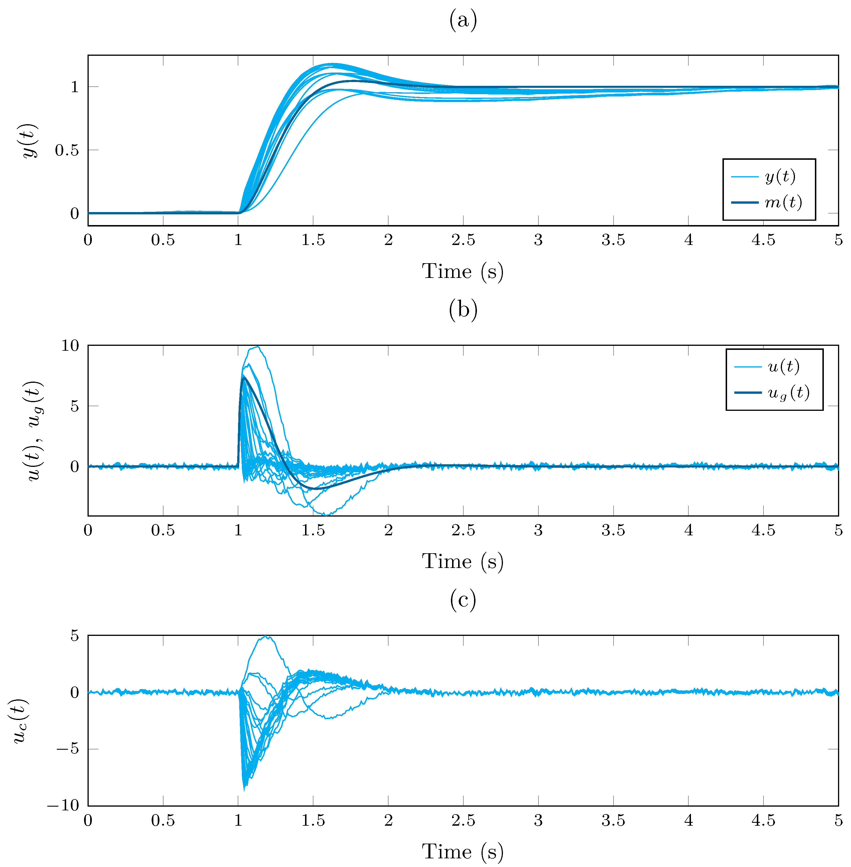
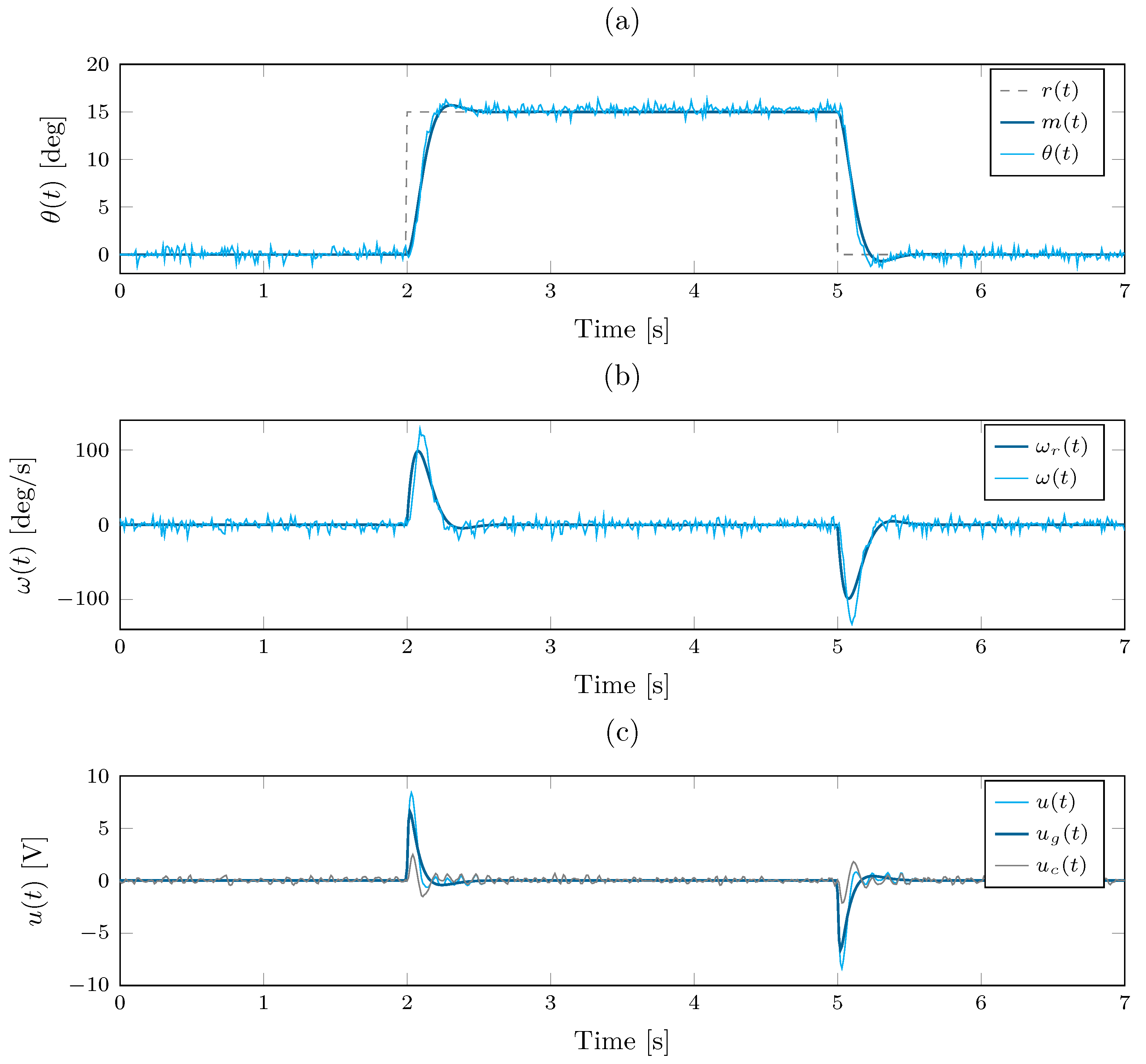
5. Validation on a Real System

Cascade structures are widely used in servo motor control [23]. This section presents the implementation of the proposed design strategy for the control of a servo motor marketed by Feedback Instruments Ltd., Crawley, UK. A permanent magnet motor is DC armature controlled by a single excitation signal $u\left(t\right)$ in the range $\pm 10$ [V]. Two analog sensors, a potentiometer and a tachogenerator, measure the state of the servo motor. Thus, the output shaft angle $\theta \left(t\right)$ [deg] and its rotational speed $\omega \left(t\right)$ [deg/s] are obtained for cascading feedback within the control architecture shown in Figure 2. The mechanical unit 33–100 is equipped with a magnetic brake, which can be adjusted manually to provide different loads. The behavior of the motor changes significantly with the applied braking torque. This results in a dynamic model with parameter uncertainty. Specifically, the motor speed response can be approximated by a first-order model

$$P_2\left(s\right)=\frac{k}{(\tau s+1)},k\in \left[28.12563.750\right],\tau \in \left[0.080.2\right],$$

(50)

and the servo position $P_1\left(s\right)$ corresponds to a pure integrator (13).

Robust tracking error (20) and robust stability (14) and (15) are required as control specifications. The desired tracking behavior is determined by the output model

$$M\left(s\right)=\frac{204.1}{(s^2+20s+204.1)}$$

(51)

and the error tolerance

$$B_r\left(\omega \right)={\left|\frac{0.2s(s+50)}{{(s+10)}^2}\right|}_{s=j\omega },$$

(52)

while the stability requirements use bounds $B_{s_1}\left(\omega \right)=B_{s_2}\left(\omega \right)=1.46$ on complementary sensitivity functions to ensure phase margins of at least ${40}^{\circ }$ in both loops.

The proposed strategy yields the feedback controllers

$$C_1\left(s\right)=\frac{5.5}{(s+5.5)},$$

(53)

$$C_2\left(s\right)=\frac{951.56(s+12.85)(s+8)}{(s+62)(s+1.3)(s^2+169.6s+1.124\times {10}^4)};$$

(54)

and the feedforward controller

$$G\left(s\right)=\frac{64.949s(s+7)}{(s^2+21.84s+161.3)(s+108)}.$$

(55)

Figure 7 shows the performance of the proposed control system in the real servomotor; the experiment corresponds to 0 % of magnetic brake. Figure 7a shows how the angle $\theta \left(t\right)$ behaves faithfully to the model $m\left(t\right)$ in tracking the reference $r\left(t\right)$. Further deviations are expected for other brake torques. However, let us remember that the tracking error is limited by the tolerance $B_r$ (52). Figure 7b shows the internal state, i.e., the rotating speed of the output shaft $\omega \left(t\right)$. The signal ${\omega }_r\left(t\right)$ sums the output of $C_1$ and the output of $M_2=sM$ and can therefore be interpreted as a virtual reference for the internal feedback loop that controls the speed. Finally, Figure 7c shows the control action $u\left(t\right)$, which attacks the DC armature circuit. This action is provided by the feedback and feedforward components, $u_c\left(t\right)$ and $u_g\left(t\right)$, respectively. Note how moderate noise affects the states $\theta \left(t\right)$ and $\omega \left(t\right)$, and the feedback action $u_c\left(t\right)$. This limited amplification of sensor noise was made possible by a smart use of feedback: first, the use of feedforward channels reduced the total amount of feedback needed, and, second, this feedback was split between two controllers.

6. Conclusions

For a given robust performance, the current work has focused on reducing the bandwidth of the feedback controllers as much as possible in order to cut off the sensor noise at the actuator. To this end, a new control architecture has been proposed. It takes advantage of two structural elements that have been used separately or suboptimally in the past. On the one hand, it is possible to feedforward the reference in tracking problems. By using a feedforward controller within a model-matching structure, the amount of feedback has been reduced to the minimum necessary for all plants in the uncertainty set to satisfy the robust tracking error specification. On the other hand, in systems where internal plant states are accessible, it is possible to close nested feedback loops. A method of frequency distribution of the total feedback between the internal and external loops has been proposed in such a way that the total sensor noise at the plant input is reduced to a minimum. All this has been done within the framework of QFT, allowing robust designs to be made using standard CAD tools. The new contributions may be particularly relevant in control systems with demanding tracking specifications and large plant uncertainties. Thus, for the sake of clarity, robust stability and reference tracking problems have been addressed in the examples. However, robust disturbance rejection could also be included in the specifications. The new proposal assumes an inner measurement that divides the plant from the control input to the controlled output into two plant models, and that no uncertainty can be defined for the outer plant model; a pure integrator is probably the most realistic case.

Two examples were presented. A theoretical example illustrated the design methodology and verified the expected control behavior. The same example then highlighted the advantages of the new architecture (double feedback plus feedforward controllers) compared to other feasible QFT solutions so far (a structure with double feedback and no feedforward, and two different structures with single feedback plus feedforward). In addition, the same case was solved by performing a non-optimal distribution of the frequency band between the two feedback loops. A total of five different cases (structures and/or loop frequency assignments) were compared with the current proposal, whose set of feedback controllers offered the least amplification of sensor noise at the plant actuator to achieve the same tracking performance. Quantitative comparisons were made using magnitude-frequency responses of the controllers and calculating representative values of total sensor noise transfer to the control input. Finally, a second example validated the new architecture and design method in practice. The angle of rotation of a commercial servo motor was successfully controlled using its speed as an internal measure.

References

1. Garcia-Sanz, M. Robust Control Engineering: Practical QFT Solutions; CRC Press: Boca Raton, FL, USA, 2017. [Google Scholar] [CrossRef]
2. Sidi, M.J. Design of Robust Control Systems: From Classical to Modern Practical Approaches; Krieger Publishing Company: Malabar, FL, USA, 2001. [Google Scholar]
3. Horowitz, I. Quantitative Feedback Design Theory (QFT); QFT Publications: Boulder, CO, USA, 1993. [Google Scholar]
4. Liu, P.; Song, Y.; Yan, P.; Sun, Y. Actuator Saturation Compensation for Fast Tool Servo Systems with Time Delays. IEEE Access 2021, 9, 6633–6641. [Google Scholar] [CrossRef]
5. Horowitz, I.; Sidi, M. Synthesis of cascaded multiple-loop feedback systems with large plant parameter ignorance. Automatica 1973, 9, 589–600. [Google Scholar] [CrossRef]
6. Marlin, T.E. Process Control: Designing Processes and Control Systems for Dynamic Performance; McGraw-Hill Science, Engineering & Mathematics: New York, NY, USA, 2000. [Google Scholar]
7. Siddiqui, M.A.; Anwar, M.; Laskar, S.; Mahboob, M. A unified approach to design controller in cascade control structure for unstable, integrating and stable processes. ISA Trans. 2021, 114, 331–346. [Google Scholar] [CrossRef]
8. Alfaro, V.; Vilanova, R.; Arrieta, O. Robust tuning of Two-Degree-of-Freedom (2-DoF) PI/PID based cascade control systems. J. Process Control 2009, 19, 1658–1670. [Google Scholar] [CrossRef]
9. Jia, B.; Mikalsen, R.; Smallbone, A.; Zuo, Z.; Feng, H.; Roskilly, A.P. Piston motion control of a free-piston engine generator: A new approach using cascade control. Appl. Energy 2016, 179, 1166–1175. [Google Scholar] [CrossRef]
10. Wu, W.; Jayasuriya, S. A new QFT design method for SISO cascaded-loop design. J. Dyn. Syst. Meas. Control Trans. ASME 2001, 123, 31–34. [Google Scholar] [CrossRef]
11. Borghesani, C.; Chait, Y.; Yaniv, O. Quantitative Feedback Theory Toolbox. For Use with Matlab, 2nd ed.; Terasoft: San Diego, CA, USA, 2002. [Google Scholar]
12. Chait, Y.; Yaniv, O. Multi-input/single-output computer-aided control design using the quantitative feedback theory. Int. J. Robust Nonlinear Control 1993, 3, 47–54. [Google Scholar] [CrossRef]
13. Eitelberg, E. Quantitative feedback design for tracking error tolerance. Automatica 2000, 36, 319–326. [Google Scholar] [CrossRef]
14. Boje, E. Pre-filter design for tracking error specifications in QFT. Int. J. Robust Nonlinear Control 2003, 13, 637–642. [Google Scholar] [CrossRef]
15. Elso, J.; Gil-Martínez, M.; García-Sanz, M. Quantitative feedback-feedforward control for model matching and disturbance rejection. IET Control Theory Appl. 2013, 7, 894–900. [Google Scholar] [CrossRef]
16. Rico-Azagra, J.; Gil-Martínez, M. Feedforward for Robust Reference Tracking in Multi-Input Feedback Control. IEEE Access 2021, 9, 92553–92567. [Google Scholar] [CrossRef]
17. Pretorius, A.; Boje, E. Robust plant by plant control design using model-error tracking sets. Int. J. Robust Nonlinear Control 2019, 29, 3330–3340. [Google Scholar] [CrossRef]
18. Jeyasenthil, R.; Kobaku, T. Quantitative Synthesis to Tracking Error Problem Based on Nominal Sensitivity Formulation. IEEE Trans. Circuits Syst. II Express Briefs 2021, 68, 2483–2487. [Google Scholar] [CrossRef]
19. Rico-Azagra, J.; Gil-Martínez, M.; Elso, J. Quantitative feedback control of multiple input single output systems. Math. Probl. Eng. 2014, 2014, 1–17. [Google Scholar] [CrossRef]
20. Gil-Martínez, M.; Rico-Azagra, J.; Elso, J. Frequency domain design of a series structure of robust controllers for multi-input single-output systems. Math. Probl. Eng. 2018, 2018. [Google Scholar] [CrossRef]
21. Rico-Azagra, J.; Gil-Martínez, M. Feedforward of measurable disturbances to improve multi-input feedback control. Mathematics 2021, 9, 2114. [Google Scholar] [CrossRef]
22. Velazquez, M.; Cruz, D.; Garcia, S.; Bandala, M. Velocity and Motion Control of a Self-Balancing Vehicle Based on a Cascade Control Strategy. Int. J. Adv. Robot. Syst. 2016, 13, 106. [Google Scholar] [CrossRef]
23. Lin, P.; Wu, Z.; Fei, Z.; Sun, X.M. A Generalized PID Interpretation for High-Order LADRC and Cascade LADRC for Servo Systems. IEEE Trans. Ind. Electron. 2022, 69, 5207–5214. [Google Scholar] [CrossRef]
24. Rico-Azagra, J.; Gil-Martínez, M.; Rico, R.; Maisterra, P. QFT bounds for robust stability specifications defined on the open-loop function. Int. J. Robust Nonlinear Control 2018, 28, 1116–1125. [Google Scholar] [CrossRef]
25. Houpis, C.; Rasmussen, S.; Garcia-Sanz, M. Quantitative Feedback Theory: Fundamentals and Applications, 3rd ed.; CRC Press: Boca Raton, FL, USA, 2006. [Google Scholar]
26. Visioli, A. Practical PID Control; Springer Science & Business Media: Berlin, Germany, 2006. [Google Scholar]
Figure 1. Earlier control architectures: (a) Cascade control, and (b) Model matching.
Mathematics 11 02523 g001
Figure 2. Cascade model matching (proposed architecture).
Mathematics 11 02523 g002
Figure 3. Bounds (colored lines) and shaping functions (black lines) for: (a) feedback controller  C 1 , (b) feedback controller  C 2 , and (c) feedforward controller G.
Mathematics 11 02523 g003
Figure 4. Magnitude frequency responses: (a) tracking error, (b) complementary sensitivity functions, (c) inner and outer open-loop functions, and (d) noise inputs to control effort.
Mathematics 11 02523 g004
Figure 5. Time-domain responses: (a) output and model output, (b) control effort and its feedforward component, and (c) feedback contribution to control effort.
Mathematics 11 02523 g005
Figure 6. Magnitude frequency responses of feedback controllers: (a) outer loop, and (b) inner loop.
Mathematics 11 02523 g006
Figure 7. Time-domain behavior: (a) angle-related responses, (b) speed-related responses, and (c) control signals.
Mathematics 11 02523 g007