Explicit Properties of Apostol-Type Frobenius–Euler Polynomials Involving q-Trigonometric Functions with Applications in Computer Modeling

Abstract

In this article, we define q-cosine and q-sine Apostol-type Frobenius–Euler polynomials and derive interesting relations. We also obtain new properties by making use of power series expansions of q-trigonometric functions, properties of q-exponential functions, and q-analogues of the binomial theorem. By using the Mathematica program, the computational formulae and graphical representation for the aforementioned polynomials are obtained. By making use of a partial derivative operator, we derived some interesting finite combinatorial sums. Finally, we detail some special cases for these results.

1. Introduction

Recently, many authors have considered and applied the generating functions techniques to new families of special polynomials, including two parametric kinds of polynomials, such as Bernoulli, Euler, Genocchi, etc. (see [1,2,3,4,5,6,7,8,9,10]). They have firstly derived the basic identities of these polynomials. Additionally, they have established more identities and relations among trigonometric functions, using two parametric kinds of polynomials by using generating functions. By applying the partial derivative operator to these generating functions, derivative formulae, and finite combinatorial sums involving the special polynomials and numbers are obtained. We would like to note that these special polynomials facilitate the derivation of various helpful properties in a fairly straightforward way and lead to introducing new families of special polynomials. The Apostol-type polynomials appear in combinatorial mathematics and play an important role in theory, generalization, applications and modeling; thus, many number theorists and combinatorics experts have extensively investigated their properties and obtained a series of interesting results (see [5,8,9,11,12,13]). Inspired by the above polynomials, in this study, we are in a position to state the parametric kinds of Apostol-type Frobenius–type Euler polynomials by introducing the two specific q-analogues of exponential generating functions. Additionally, we prove many formulas and relations for these polynomials, including some implicit summation formulas, differentiation rules and correlations with the earlier polynomials by utilizing some series manipulation methods. Additionally, as an application, we show the zero values of q-Apostol-type Frobenius–type Euler polynomials using tables and draw some graphical representations.

We begin by stating the following definitions and notations of q-calculus reviewed here, which are taken from (see [14]):

A q-analogue of the shifted factorial ${\left(a\right)}_n$ is given by

$${(a;q)}_0=1,{(a;q)}_n=\prod _{m=0}^{n-1}(1-q^{m}a),\hspace{0.17em}n\in \mathbb{N}.$$

A q-analogue of a complex number a and of the factorial function are given by

$${\left[a\right]}_q=\frac{1-q^a}{1-q},(q\in \mathbb{C}\backslash \left\{1\right\};a\in \mathbb{C}),$$

$${\left[n\right]}_q!=\prod _{m=1}^n{\left[m\right]}_q={\left[1\right]}_q{\left[2\right]}_q\cdots {\left[n\right]}_q=\frac{{(q;q)}_n}{{(1-q)}^n},q\ne 1;n\in \mathbb{N},$$

$${\left[0\right]}_q!=1,q\in \mathbb{C};0<\mid q\mid <1.$$

The Gauss q-binomial coefficient ${\left(\begin{array}{c}n\\ k\end{array}\right)}_q$ is given by

$${\left(\begin{array}{c}n\\ k\end{array}\right)}_q=\frac{{\left[n\right]}_q!}{{\left[k\right]}_q!{[n-k]}_q!}=\frac{{(q;q)}_n}{{(q;q)}_k{(q;q)}_{n-k}},k=0,1,\cdots ,n.$$

The q-analogue of the function ${(x+y)}_q^n$ is given by

$${(x+y)}_q^n=\sum _{k=0}^n{\left(\begin{array}{c}n\\ k\end{array}\right)}_q{q}^{k(k-1)/2}{x}^{n-k}{y}^k,n\in {\mathbb{N}}_0.$$

(1)

The q-analogues of exponential functions are given by

$$e_q\left(x\right)=\sum _{n=0}^{\infty }\frac{x^n}{{\left[n\right]}_q!}=\frac{1}{{((1-q)x;q)}_{\infty }},0<\mid q\mid <1;\mid x\mid <\mid 1-q{\mid }^{-1},$$

(2)

$$E_q\left(x\right)=\sum _{n=0}^{\infty }\frac{q^{(\frac{n}{2})}}{{\left[n\right]}_q!}{x}^n={(-(1-q)x;q)}_{\infty },0<\mid q\mid <1;x\in \mathbb{C}.$$

(3)

These two functions are related by the equation (see [14])

$$e_q\left(x\right)E_q(-x)=1.$$

A q-derivative operator of a function is defined by

$$D_{q,z}f\left(z\right):=D_{q}f\left(z\right)=\frac{f\left(qz\right)-f\left(z\right)}{qz-z},0<\mid q\mid <1,$$

and $D_{q}f\left(0\right)=f^{\prime }\left(0\right)$ provided that f is differentiable at $x=0$.

A q-derivative fulfills the following product and quotient rules

$$D_{q,z}\left(f\left(z\right)g\left(z\right)\right)=f\left(z\right)D_{q,z}g\left(z\right)+g\left(qz\right)D_{q,z}f\left(z\right),$$

(4)

$$D_{q,z}\left(\frac{f\left(z\right)}{g\left(z\right)}\right)=\frac{g\left(qz\right)D_{q,z}f\left(z\right)-f\left(qz\right)D_{q,z}g\left(z\right)}{g\left(z\right)g\left(qz\right)}.$$

(5)

The Apostol-type q-Bernoulli polynomials ${\mathbb{B}}_{n,q}^{\left(\alpha \right)}(x;\lambda )$ of order $\alpha$, the Apostol-type q-Euler polynomials ${\mathbb{E}}_{n,q}^{\left(\alpha \right)}(x;\lambda )$ of order $\alpha$ and the Apostol-type q-Genocchi polynomials ${\mathbb{G}}_{n,q}^{\left(\alpha \right)}(x;\lambda )$ of order $\alpha$ are defined by (see [15,16]):

$${\left(\frac{t}{\lambda e_q\left(t\right)-1}\right)}^{\alpha }{e}^{xt}=\sum _{n=0}^{\infty }{\mathbb{B}}_{n,q}^{\left(\alpha \right)}(x;\lambda )\frac{t^n}{{\left[n\right]}_q!},$$

(6)

$${\left(\frac{2}{\lambda e_q\left(t\right)+1}\right)}^{\alpha }{e}^{xt}=\sum _{n=0}^{\infty }{\mathbb{E}}_{n,q}^{\left(\alpha \right)}(x;\lambda )\frac{t^n}{{\left[n\right]}_q!},$$

(7)

$${\left(\frac{2t}{\lambda e_q\left(t\right)+1}\right)}^{\alpha }{e}^{xt}=\sum _{n=0}^{\infty }{\mathbb{G}}_{n,q}^{\left(\alpha \right)}(x;\lambda )\frac{t^n}{{\left[n\right]}_q!},$$

(8)

respectively.

Clearly, we can obtain

$${\mathbb{B}}_{n,q}^{\left(\alpha \right)}\left(\lambda \right)={\mathbb{B}}_{n,q}^{\left(\alpha \right)}(0;\lambda ),{\mathbb{E}}_{n,q}^{\left(\alpha \right)}\left(\lambda \right)={\mathbb{E}}_{n,q}^{\left(\alpha \right)}(0;\lambda ),{\mathbb{G}}_{n,q}^{\left(\alpha \right)}\left(\lambda \right)={\mathbb{G}}_{n,q}^{\left(\alpha \right)}(0;\lambda ),$$

and

$${\mathbb{B}}_{n,q}^{\left(1\right)}(x;\lambda )={\mathbb{B}}_{n,q}(x;\lambda ),{\mathbb{E}}_{n,q}^{\left(1\right)}(x;\lambda )={\mathbb{E}}_{n,q}(x;\lambda ),{\mathbb{G}}_{n,q}^{\left(1\right)}(x;\lambda )={\mathbb{G}}_{n,q}(x;\lambda ).$$

Let $u\in \mathbb{C}$ with $u\ne 1$ and $\xi \in \mathbb{R}$. The Apostol-type q-Frobenius–Euler polynomials ${\mathbb{H}}_{n,q}^{\left(\alpha \right)}(x,y;u;\lambda )$ of order $\alpha \in \mathbb{C}$ are defined by (see [11,12]):

$${\left(\frac{1-u}{\lambda e_q\left(t\right)-u}\right)}^{\alpha }{e}_q\left(xt\right)E_q\left(yt\right)=\sum _{n=0}^{\infty }{\mathbb{H}}_{n,q}^{\left(\alpha \right)}(x,y;u;\lambda )\frac{t^n}{{\left[n\right]}_q!},\left|z\right|<\left|ln,\left(\frac{\lambda }{u}\right)\right|.$$

(9)

It is obvious that

$${\mathbb{H}}_{n,q}^{\left(\alpha \right)}(u;\lambda )={\mathbb{H}}_{n,q}^{\left(\alpha \right)}(0,0;u;\lambda )\underset{q\to 1^{-}}{lim}{\mathbb{H}}_{n,q}^{\left(\alpha \right)}(x,y;u;\lambda )={\mathbb{H}}_n^{\left(\alpha \right)}(x+y;u;\lambda ).$$

Kang et al. [2,4] introduced the q-Bernoulli and q-Euler polynomials defined by

$$\frac{z}{e_q\left(z\right)-1}{e}_q\left(\xi z\right)CO{S}_q\left(\eta z\right)=\sum _{j=0}^{\infty }\frac{{\mathbb{B}}_{j,q}({(\xi +i\eta )}_q)+{\mathbb{B}}_j({(\xi -i\eta )}_q)}{2}\frac{z^j}{{\left[j\right]}_q!}=\sum _{j=0}^{\infty }{\mathbb{B}}_{j,q}^{\left(C\right)}(\xi ,\eta )\frac{z^j}{{\left[j\right]}_q!},$$

(10)

$$\frac{z}{e_q\left(z\right)-1}{e}_q\left(\xi z\right)SI{N}_q\left(\eta z\right)=\sum _{j=0}^{\infty }\frac{{\mathbb{B}}_{j,q}({(\xi +i\eta )}_q)-{\mathbb{B}}_{j,q}({(\xi -i\eta )}_q)}{2i}\frac{z^j}{{\left[j\right]}_q!}=\sum _{j=0}^{\infty }{\mathbb{B}}_{j,q}^{\left(S\right)}(\xi ,\eta )\frac{z^j}{{\left[j\right]}_q!},$$

(11)

and

$$\frac{2}{e_q\left(z\right)+1}{e}_q\left(\xi z\right)CO{S}_q\left(\eta z\right)=\sum _{j=0}^{\infty }\frac{{\mathbb{E}}_{j,q}({(\xi +i\eta )}_q)+{\mathbb{E}}_{j,q}({(\xi -i\eta )}_q)}{2}\frac{z^j}{{\left[j\right]}_q!}=\sum _{j=0}^{\infty }{\mathbb{E}}_{j,q}^{\left(C\right)}(\xi ,\eta )\frac{z^j}{{\left[j\right]}_q!},$$

(12)

$$\frac{2}{e_q\left(z\right)+1}{e}_q\left(\xi z\right)SI{N}_q\left(\eta z\right)=\sum _{j=0}^{\infty }\frac{{\mathbb{E}}_j({(\xi +i\eta )}_q)-{\mathbb{E}}_j{((\xi -i\eta ))}_q}{2i}\frac{z^j}{{\left[j\right]}_q!}=\sum _{j=0}^{\infty }{\mathbb{E}}_{j,q}^{\left(S\right)}(\xi ,\eta )\frac{z^j}{{\left[j\right]}_q!},$$

(13)

respectively.

Additionally, they have proved that (see [2,4]):

$$e_q\left(\xi z\right)CO{S}_q\left(\eta z\right)=\sum _{r=0}^{\infty }{C}_{r,q}(\xi ,\eta )\frac{z^r}{{\left[r\right]}_q!},$$

(14)

and

$$e_q\left(\xi z\right)SI{N}_q\left(\eta z\right)=\sum _{r=0}^{\infty }{S}_{r,q}(\xi ,\eta )\frac{z^r}{{\left[r\right]}_q!},$$

(15)

where

$$C_{r,q}(\xi ,\eta )=\sum _{j=0}^{\left[\frac{r}{2}\right]}{\left(\begin{array}{c}r\hfill \\ 2j\hfill \end{array}\right)}_q{(-1)}^j{q}^{2j-1}{\xi }^{r-2j}{\eta }^{2j},$$

(16)

and

$$S_{r,q}(\xi ,\eta )=\sum _{j=0}^{[\frac{r-1}{2}]}{\left(\begin{array}{c}r\hfill \\ 2j+1\hfill \end{array}\right)}_q{(-1)}^j{q}^{(2j+1)j}{\xi }^{r-2j-1}{\eta }^{2j+1}.$$

(17)

2. q-Apostol-Type Frobenius–Euler Polynomials of Complex Variable

In this section, we consider the q-Cosine and q-Sine Apostol-type Frobenius–Euler polynomials of a complex variable and deduce some identities of these polynomials. First, we present the following definition.

$${\left(\frac{1-u}{\lambda e_q\left(t\right)-u}\right)}^{\alpha }{e}_q\left(xt\right)E_q\left(ity\right)=\sum _{n=0}^{\infty }{\mathbb{H}}_{n,q}^{\left(\alpha \right)}({(\xi +iy)}_q;u;\lambda )\frac{t^n}{{\left[n\right]}_q!}.$$

(18)

It is well-known from ([4] Definition 5) that

$$e_q\left(xt\right)E_q\left(ity\right)=e_q\left(xt\right)(CO{S}_q\left(yt\right)+iSI{N}_q\left(yt\right)).$$

(19)

Thus, by (18) and (19), we have

$$\sum _{n=0}^{\infty }{\mathbb{H}}_{n,q}^{\left(\alpha \right)}({(x+iy)}_q;u;\lambda )\frac{t^n}{n!}={\left(\frac{1-u}{\lambda e_q\left(t\right)-u}\right)}^{\alpha }{e}_q\left(xt\right)E_q\left(ity\right)$$

$$={\left(\frac{1-u}{\lambda e_q\left(t\right)-u}\right)}^{\alpha }{e}_q\left(xt\right)(CO{S}_q\left(yz\right)+iSI{N}_q\left(yz\right)),$$

(20)

and

$$\sum _{n=0}^{\infty }{\mathbb{H}}_{n,q}^{\left(\alpha \right)}({(x-iy)}_q;u;\lambda )\frac{t^n}{{\left[n\right]}_q!}={\left(\frac{1-u}{\lambda e_q\left(t\right)-u}\right)}^{\alpha }{e}_q\left(xt\right)E_q(-ity)$$

$$={\left(\frac{1-u}{\lambda e_q\left(t\right)-u}\right)}^{\alpha }{e}_q\left(xt\right)(CO{S}_q\left(yt\right)-iSI{N}_q\left(yt\right)).$$

(21)

From (20) and (21), we get

$${\left(\frac{1-u}{\lambda e_q\left(t\right)-u}\right)}^{\alpha }{e}_q\left(xt\right)CO{S}_q\left(yt\right)=\sum _{n=0}^{\infty }\left(\frac{{\mathbb{H}}_{n,q}^{\left(\alpha \right)}({(x+iy)}_q;u;\lambda )+{\mathbb{H}}_{n,q}^{\left(\alpha \right)}({(x-iy)}_q;u;\lambda )}{2}\right)\frac{t^n}{{\left[n\right]}_q!},$$

(22)

and

$${\left(\frac{1-u}{\lambda e_q\left(t\right)-u}\right)}^{\alpha }{e}_q\left(xt\right)SI{N}_q\left(yt\right)=\sum _{n=0}^{\infty }\left(\frac{{\mathbb{H}}_{n,q}^{\left(\alpha \right)}({(x+iy)}_q;u;\lambda )-{\mathbb{H}}_{n,q}^{\left(\alpha \right)}({(x-iy)}_q;u;\lambda )}{2}\right)\frac{t^n}{{\left[n\right]}_q!}.$$

(23)

Definition 1.

Let $j\ge 0$. We define two parametric kinds of q-Cosine Apostol-type Frobenius–Euler polynomials ${\mathbb{H}}_{n,q}^{(\alpha ,c)}(x,y;u;\lambda )$ and q-Sine Apostol-type Frobenius–Euler polynomials ${\mathbb{H}}_{n,q}^{(\alpha ,s)}(x,y;u;\lambda )$, for a non negative integer n, by

$${\left(\frac{1-u}{\lambda e_q\left(t\right)-u}\right)}^{\alpha }{e}_q\left(xt\right)CO{S}_q\left(yt\right)=\sum _{n=0}^{\infty }{\mathbb{H}}_{j,q}^{(\alpha ,c)}(x,y;u;\lambda )\frac{t^n}{{\left[n\right]}_q!},$$

(24)

and

$${\left(\frac{1-u}{\lambda e_q\left(t\right)-u}\right)}^{\alpha }{e}_q\left(xt\right)SI{N}_q\left(yt\right)=\sum _{n=0}^{\infty }{\mathbb{H}}_{n,q}^{(\alpha ,s)}(x,y;u;\lambda )\frac{t^n}{{\left[n\right]}_q!},$$

(25)

respectively.

Note that ${\mathbb{H}}_{n,q}^{(\alpha ,c)}(0,0;u;\lambda )={\mathbb{H}}_{n,q}(u;\lambda ),{\mathbb{H}}_{n,q}^{(\alpha ,s)}(0,0;u;\lambda )=0,(n\ge 0)$.

From (22)–(25), we have

$${\mathbb{H}}_{n,q}^{(\alpha ,c)}(x,y;u;\lambda )=\frac{{\mathbb{H}}_{n,q}({(x+iy)}_q;u;\lambda )+{\mathbb{H}}_{n,q}({(x-iy)}_q;u;\lambda )}{2},$$

(26)

$${\mathbb{H}}_{n,q}^{(\alpha ,s)}(x,y;u;\lambda )=\frac{{\mathbb{H}}_{n,q}({(x+iy)}_q;u;\lambda )-{\mathbb{H}}_{n,q}({(x-iy)}_q;u;\lambda )}{2i}.$$

(27)

Remark 1.

For $x=0$ in (24) and (25), we obtain

$${\left(\frac{1-u}{\lambda e^t-u}\right)}^{\alpha }CO{S}_q\left(yt\right)=\sum _{j=0}^{\infty }{\mathbb{H}}_{n,q}^{(\alpha ,c)}(y;u;\lambda )\frac{t^n}{{\left[n\right]}_q!},$$

(28)

and

$${\left(\frac{1-u}{\lambda e^t-u}\right)}^{\alpha }SI{N}_q\left(yt\right)=\sum _{n=0}^{\infty }{\mathbb{H}}_{n,q}^{(\alpha ,s)}(y;u;\lambda )\frac{t^n}{{\left[n\right]}_q!},$$

(29)

respectively.

It is clear that

$${\mathbb{H}}_{n,q}^{(\alpha ,c)}(0;u;\lambda )={\mathbb{H}}_{n,q}(u;\lambda ),{\mathbb{H}}_{n,q}^{(\alpha ,s)}(0;u;\lambda )=0,(n\ge 0).$$

Now, we provide some basic properties of these polynomials.

Theorem 1.

Let $n\ge 0$. Then,

$${\mathbb{H}}_{n,q}^{(\alpha ,c)}(y;u;\lambda )=\sum _{v=0}^{\left[\frac{n}{2}\right]}{\left(\begin{array}{c}n+v\hfill \\ 2v\hfill \end{array}\right)}_q{(-1)}^v{q}^{(2v-1)v}{y}^{2v}{\mathbb{H}}_{n-2v,q}(u;\lambda ),$$

(30)

and

$${\mathbb{H}}_{j,q}^{(\alpha ,s)}(u;\lambda )=\sum _{v=0}^{[\frac{n-1}{2}]}{\left(\begin{array}{c}n+v\hfill \\ 2v+1\hfill \end{array}\right)}_q{(-1)}^v{q}^{(2v+1)v}{y}^{2v+1}{\mathbb{H}}_{n-2v-1,q}(u;\lambda ).$$

(31)

Proof. 

By (28) and (29), we can derive the following equations

$$\sum _{n=0}^{\infty }{\mathbb{H}}_{n,q}^{(\alpha ,c)}(y;u;\lambda )\frac{t^n}{{\left[n\right]}_q!}={\left(\frac{1-u}{\lambda e_q\left(t\right)-u}\right)}^{\alpha }CO{S}_q\left(yt\right)$$

$$=\sum _{n=0}^{\infty }{\mathbb{H}}_{n,q}^{\left(\alpha \right)}(u;\lambda )\frac{t^n}{{\left[n\right]}_q!}\sum _{v=0}^{\infty }{(-1)}^v{q}^{(2v-1)v}{y}^{2v}\frac{t^v}{{\left[2v\right]}_q!}.$$

$$=\sum _{n=0}^{\infty }\left(\sum _{v=0}^{\left[\frac{n}{2}\right]},{\left(\begin{array}{c}n+v\hfill \\ 2v\hfill \end{array}\right)}_q,{(-1)}^v,q^{(2v-1)v},y^{2v},{\mathbb{H}}_{n-2v,q},(u;\lambda )\right)\frac{t^n}{{\left[n\right]}_q!},$$

(32)

and

$$\sum _{n=0}^{\infty }{\mathbb{H}}_{n,q}^{(\alpha ,s)}(y;u;\lambda )\frac{t^n}{n!}={\left(\frac{1-u}{\lambda e_q\left(t\right)-u}\right)}^{\alpha }SI{N}_q\left(yt\right)$$

$$=\sum _{n=0}^{\infty }\left(\sum _{v=0}^{[\frac{n-1}{2}]},{\left(\begin{array}{c}n\hfill \\ 2v+1\hfill \end{array}\right)}_q,{(-1)}^v,q^{(2v+1)v},y^{2v+1},{\mathbb{H}}_{j-2v-1,q},(u;\lambda )\right)\frac{t^n}{{\left[n\right]}_q!}.$$

(33)

Therefore, with (32) and (33), we get (30) and (31). □

Theorem 2.

Let $n\ge 0$. Then,

$${\mathbb{H}}_{n,q}^{\left(\alpha \right)}({(x+iy)}_q;u;\lambda )=\sum _{k=0}^n{\left(\genfrac{}{}{0pt}{}{n}{k}\right)}_q{(x+iy)}_q^k{\mathbb{H}}_{n-k,q}^{\left(\alpha \right)}(u;\lambda )$$

$$=\sum _{k=0}^n{\left(\genfrac{}{}{0pt}{}{n}{k}\right)}_q{\left(iy\right)}^k{\mathbb{H}}_{j-k,q}^{\left(\alpha \right)}(x;u;\lambda ),$$

(34)

and

$${\mathbb{H}}_{n,q}^{\left(\alpha \right)}({(x-iy)}_q;u;\lambda )=\sum _{k0}^n{\left(\genfrac{}{}{0pt}{}{n}{k}\right)}_q{(x-iy)}_q^k{\mathbb{H}}_{n-k,q}^{\left(\alpha \right)}(u;\lambda )$$

$$=\sum _{k=0}^n{\left(\genfrac{}{}{0pt}{}{n}{k}\right)}_q{(-1)}^k{\left(iy\right)}^k{\mathbb{H}}_{n-k,q}(x;u;\lambda ).$$

(35)

Proof. 

By using (20) and (21), we obtain (34) and (35). So, we omit the proof. □

Theorem 3.

Let $n\ge 0$. Then,

$${\mathbb{H}}_{n,q}^{(\alpha ,c)}(x,y;u;\lambda )=\sum _{k=0}^n{\left(\begin{array}{c}n\\ k\end{array}\right)}_q{\mathbb{H}}_{k,q}^{\left(\alpha \right)}(u;\lambda )C_{n-k,q}(x,y),$$

(36)

and

$${\mathbb{H}}_{n,q}^{(\alpha ,s)}(x,y;u;\lambda )=\sum _{k=0}^n{\left(\begin{array}{c}n\\ k\end{array}\right)}_q{\mathbb{H}}_{k,q}(u;\lambda )S_{n-k,q}(x,y).$$

(37)

Proof. 

Consider

$$\left(\sum _{n=0}^{\infty },a_n,\frac{t^n}{n!}\right)\left(\sum _{k=0}^{\infty },b_k,\frac{t^k}{k!}\right)=\sum _{n=0}^{\infty }\left(\sum _{k=0}^j,a_{n-k},b_k\right)\frac{t^n}{n!}.$$

Now,

$$\sum _{n=0}^{\infty }{\mathbb{H}}_{j,q}^{(\alpha ,c)}(x,y;u;\lambda )\frac{t^n}{{\left[n\right]}_q!}={\left(\frac{1-u}{\lambda e_q\left(t\right)-u}\right)}^{\alpha }{e}_q\left(xt\right)CO{S}_q\left(yt\right)$$

$$=\left(\sum _{k=0}^{\infty },{\mathbb{H}}_{k,q}^{\left(\alpha \right)},(u;\lambda ),\frac{t^k}{k!}\right)\left(\sum _{n=0}^{\infty },C_{n,q},(x,y),\frac{t^n}{{\left[n\right]}_q!}\right)$$

$$=\sum _{n=0}^{\infty }\left(\sum _{k=0}^n,{\left(\begin{array}{c}n\\ k\end{array}\right)}_q,{\mathbb{H}}_{k,q}^{\left(\alpha \right)},(u;\lambda ),C_{n-k,q},(x,y)\right)\frac{t^n}{{\left[n\right]}_q!},$$

which proves (36). The proof of (37) is similar.

□

By using Definition 1, we can easily obtain the following Theorems. So, we omit the proofs.

Theorem 4.

Let $j\ge 0$. Then,

$${\mathbb{H}}_{j,q}^{(\alpha ,c)}(x+s,y;u;\lambda )=\sum _{k=0}^n{\left(\begin{array}{c}n\\ k\end{array}\right)}_q{\mathbb{H}}_{k,q}^{(\alpha ,c)}(x,y;u;\lambda )r^{n-k},$$

(38)

and

$${\mathbb{H}}_{n,q}^{(\alpha ,s)}(x,y;u;\lambda )=\sum _{k=0}^n{\left(\begin{array}{c}n\\ k\end{array}\right)}_q{\mathbb{H}}_{k,q}^{(\alpha ,s)}(x,y;u;\lambda )r^{n-k}.$$

(39)

Theorem 5.

Let $j\ge 1$. Then,

$$\frac{\partial }{\partial x}{\mathbb{H}}_{n,q}^{(\alpha ,c)}(x,y;u;\lambda )={\left[n\right]}_q{\mathbb{H}}_{n-1,q}^{(\alpha ,c)}(x,y;u;\lambda ),$$

(40)

$$\frac{\partial }{\partial y}{\mathbb{H}}_{n,q}^{(\alpha ,c)}(x,y;u;\lambda )=-{\left[n\right]}_q{\mathbb{H}}_{n-1,q}^{(\alpha ,s)}(x,qy;u;\lambda ),$$

(41)

and

$$\frac{\partial }{\partial x}{\mathbb{H}}_{n,q}^{(\alpha ,s)}(x,y;u;\lambda )={\left[n\right]}_q{\mathbb{H}}_{n-1,q}^{(\alpha ,s)}(x,y;u;\lambda ),$$

(42)

$$\frac{\partial }{\partial y}{\mathbb{H}}_{n,q}^{(\alpha ,s)}(x,y;u;\lambda )={\left[n\right]}_q{\mathbb{H}}_{n-1,q}^{(\alpha ,c)}(x,qy;u;\lambda ).$$

(43)

Theorem 6.

Let n be a nonnegative integer, the following formulas hold true.

$$\lambda {\mathbb{H}}_{n,q}^{(\alpha ,c)}(1,y;u;\lambda )-u{\mathbb{H}}_{n,q}^{(\alpha ,c)}(0,y;u;\lambda )$$

$$=(1-u){\mathbb{H}}_{n,q}^{(\alpha -1,c)}(0;y;u;\lambda ),$$

(44)

$$\lambda {\mathbb{H}}_{n,q}^{(\alpha ,s)}(1,y;u;\lambda )-u{\mathbb{H}}_{n,q}^{(\alpha ,s)}(0,y;u;\lambda )$$

$$=(1-u){\mathbb{H}}_{n,q}^{(\alpha -1,s)}(0;y;u;\lambda ),$$

(45)

Theorem 7.

The following relations hold true.

$${\mathbb{H}}_{n,q}^{(\alpha +\beta ,c)}(x,y;u;\lambda )=\sum _{m=0}^n{\left(\genfrac{}{}{0pt}{}{n}{m}\right)}_q{\mathbb{H}}_{n-m,q}^{(\alpha ,c)}(x,y;u;\lambda ){\mathbb{H}}_{m,q}^{(\beta )}(u;\lambda ),$$

(46)

$${\mathbb{H}}_{n,q}^{(\alpha +\beta ,s)}(x,y;u;\lambda )=\sum _{m=0}^n{\left(\genfrac{}{}{0pt}{}{n}{m}\right)}_q{\mathbb{H}}_{n-m,q}^{(\alpha ,s)}(x,y;u;\lambda ){\mathbb{H}}_{m,q}^{(\beta )}(u;\lambda ),$$

(47)

$${\mathbb{H}}_{n,q}^{(\alpha -\beta ,c)}(x,y;u;\lambda )=\sum _{m=0}^n{\left(\genfrac{}{}{0pt}{}{n}{m}\right)}_q{\mathbb{H}}_{n-m,q}^{(\alpha ,c)}(x,y;u;\lambda ){\mathbb{H}}_{m,q}^{(-\beta )}(u;\lambda ),$$

(48)

$${\mathbb{H}}_{n,q}^{(\alpha -\beta ,s)}(x,y;u;\lambda )=\sum _{m=0}^n{\left(\genfrac{}{}{0pt}{}{n}{m}\right)}_q{\mathbb{H}}_{n-m,q}^{(\alpha ,s)}(x,y;u;\lambda ){\mathbb{H}}_{m,q}^{(-\beta )}(u;\lambda ),$$

(49)

Theorem 8.

Let $x,y,$ and r be any real numbers. Then, we have

(i) 

$${\mathbb{H}}_{n,q}^{(\alpha ,c)}({(x+r)}_q,y;u;\lambda )+{\mathbb{H}}_{n,q}^{(\alpha ,s)}({(x-r)}_q,y;u;\lambda )$$

$$=\sum _{k=0}^n{\left(\genfrac{}{}{0pt}{}{n}{l}\right)}_q{q}^{(\genfrac{}{}{0pt}{}{n-l}{2})}{r}^{n-l}\left({\mathbb{H}}_{n,q}^{(\alpha ,c)},(x,y;u;\lambda ),+,{(-1)}^{n-k},{\mathbb{H}}_{n,q}^{(\alpha ,s)},(x,y;u;\lambda )\right),$$

(50)

(ii) 

$${\mathbb{H}}_{n,q}^{(\alpha ,s)}({(x+r)}_q,y;u;\lambda )+{\mathbb{H}}_{n,q}^{(\alpha ,c)}({(x-r)}_q,y;u;\lambda )$$

$$=\sum _{k=0}^n{\left(\genfrac{}{}{0pt}{}{n}{l}\right)}_q{q}^{(\genfrac{}{}{0pt}{}{n-l}{2})}{r}^{n-l}\left({\mathbb{H}}_{n,q}^{(\alpha ,s)},(x,y;u;\lambda ),+,{(-1)}^{n-k},{\mathbb{H}}_{n,q}^{(\alpha ,c)},(x,y;u;\lambda )\right).$$

(51)

Corollary 1.

Let $j\ge 0$. Then,

$${\mathbb{H}}_{n,q}^{\left(c\right)}({(x+r)}_q,y;u;\lambda )+{\mathbb{H}}_{n,q}^{\left(c\right)}({(x-r)}_q,y;u;\lambda )$$

$$=\sum _{k=0}^n{\left(\genfrac{}{}{0pt}{}{n}{k}\right)}_q{q}^{(\genfrac{}{}{0pt}{}{k}{2})}{r}^k\left({\mathbb{H}}_{n-k,q}^{\left(c\right)},(x,y;u;\lambda ),+,{(-1)}^k,{\mathbb{H}}_{n-k,q}^{\left(c\right)},(x,y;u;\lambda )\right),$$

(52)

and

$${\mathbb{H}}_{n,q}^{\left(s\right)}({(x+r)}_q,y;u;\lambda )+{\mathbb{H}}_{n,q}^{\left(s\right)}({(x-r)}_q,y;u;\lambda )$$

$$=\sum _{k=0}^n{\left(\genfrac{}{}{0pt}{}{n}{k}\right)}_q{q}^{(\genfrac{}{}{0pt}{}{k}{2})}{r}^k\left({\mathbb{H}}_{n-k,q}^{\left(s\right)},(x,y;u;\lambda ),+,{(-1)}^k,{\mathbb{H}}_{n-k,q}^{\left(s\right)},(x,y;u;\lambda )\right).$$

(53)

Corollary 2.

For $r=1$ in Theorem 8, we obtain

$${\mathbb{H}}_{n,q}^{\left(c\right)}({(x+1)}_q,y;u;\lambda )+{\mathbb{H}}_{n,q}^{\left(s\right)}({(x-1)}_q,y;u;\lambda )$$

$$=\sum _{k=0}^n{\left(\genfrac{}{}{0pt}{}{n}{k}\right)}_q{q}^{(\genfrac{}{}{0pt}{}{k}{2})}{r}^k\left({\mathbb{H}}_{n-k,q}^{\left(c\right)},(x,y;u;\lambda ),+,{(-1)}^k,{\mathbb{H}}_{n-k,q}^{\left(s\right)},(x,y;u;\lambda )\right),$$

(54)

and

$${\mathbb{H}}_{n,q}^{\left(s\right)}({(x+1)}_q,y;u;\lambda )+{\mathbb{H}}_{n,q}^{\left(c\right)}({(x-1)}_q,y;u;\lambda )$$

$$=\sum _{k=0}^n{\left(\genfrac{}{}{0pt}{}{n}{k}\right)}_q{q}^{(\genfrac{}{}{0pt}{}{n-k}{2})}{r}^{n-k}\left({\mathbb{H}}_{k,q}^{\left(s\right)},(x,y;u;\lambda ),+,{(-1)}^{n-k},{\mathbb{H}}_{k,q}^{\left(c\right)},(x,y;u;\lambda )\right).$$

(55)

3. Summation Formulas for q-Cosine and q-Sine Apostol-Type Frobenius–Euler Polynomials

In this section, we derive some correlations for the q-cosine and q-sine Apostol-type Frobenius–Euler polynomials of order $\alpha$ associated with the q-Bernoulli, Euler, and Genocchi polynomials and the q-Stirling numbers of the second kind. We first provide the following theorems.

Theorem 9.

The following results hold true:

$$(2u-1)\sum _{k=0}^n{\left(\begin{array}{c}n\\ k\end{array}\right)}_q{\mathbb{H}}_{k,q}(x,0;u;\lambda ){\mathbb{H}}_{n-k,q}^{\left(c\right)}(0,y;1-u;\lambda )$$

$$=u{\mathbb{H}}_{n,q}^{\left(c\right)}(x,y;u;\lambda )-(1-u){\mathbb{H}}_{n,q}^{\left(c\right)}(x,y;1-u;\lambda ),$$

(56)

and

$$(2u-1)\sum _{k=0}^n{\left(\begin{array}{c}n\\ k\end{array}\right)}_q{\mathbb{H}}_{k,q}(x,0;u;\lambda ){\mathbb{H}}_{n-k,q}^{\left(s\right)}(0,y;1-u;\lambda )$$

$$=u{\mathbb{H}}_{n,q}^{\left(s\right)}(x,y;u;\lambda )-(1-u){\mathbb{H}}_{n,q}^{\left(s\right)}(x,y;1-u;\lambda ).$$

(57)

Proof. 

We set

$$\frac{(2u-1)}{(\lambda e_q\left(t\right)-u)(\lambda e_q\left(t\right)-(1-u))}=\frac{1}{\lambda e_q\left(t\right)-u}-\frac{1}{\lambda e_q\left(t\right)-(1-u)}.$$

From the above equation, we see that

$$(2u-1)\frac{(1-u)e_q\left(xt\right)(1-(1-u))CO{S}_q\left(yt\right)}{(\lambda e_q\left(t\right)-u)(\lambda e_q\left(t\right)-(1-u))}$$

$$=\frac{(1-u)e_q\left(xt\right)uCO{S}_q\left(yt\right)}{\lambda e_q\left(t\right)-u}-\frac{(1-u)e_q\left(xt\right)CO{S}_q\left(yt\right)(1-(1-u))}{\lambda e_q\left(t\right)-(1-u)},$$

which when using Equations (9) and (24) on both sides, we can obtain

$$(2u-1)\left(\sum _{k=0}^{\infty },{\mathbb{H}}_{k,q},(x,0;u;\lambda ),\frac{t^k}{{\left[k\right]}_q!}\right)\left(\sum _{n=0}^{\infty },{\mathbb{H}}_{n,q}^{\left(c\right)},(0,y;1-u;\lambda ),\frac{t^n}{{\left[n\right]}_q!}\right)$$

$$=u\sum _{n=0}^{\infty }{\mathbb{H}}_{n,q}^{\left(c\right)}(x,y;u;\lambda )\frac{t^n}{{\left[n\right]}_q!}-(1-u)\sum _{n=0}^{\infty }{\mathbb{H}}_{n,q}^{\left(c\right)}(x,y;1-u;\lambda )\frac{t^n}{{\left[n\right]}_q!}.$$

By applying the Cauchy product rule in the above equation and then equating the coefficients of like powers of t on both sides of the resultant equation, assertion (56) follows. Similarly, we obtain (57). □

Theorem 10.

The following relations hold true:

$$u{\mathbb{H}}_{n,q}^{\left(c\right)}(x,y;u;\lambda )=\sum _{k=0}^n{\left(\begin{array}{c}n\\ k\end{array}\right)}_q{\mathbb{H}}_{n,q}^{\left(c\right)}(x,y;u;\lambda )-(1-u)C_{n,q}(x,y),$$

(58)

and

$$u{\mathbb{H}}_{n,q}^{\left(s\right)}(x,y;u;\lambda )=\sum _{k=0}^n{\left(\begin{array}{c}n\\ k\end{array}\right)}_q{\mathbb{H}}_{n,q}^{\left(s\right)}(x,y;u;\lambda )-(1-u)S_{n,q}(x,y).$$

(59)

Proof. 

Consider the following identity

$$\frac{u}{\lambda (\lambda e_q\left(t\right)-u)e_q\left(t\right)}=\frac{1}{(\lambda e_q\left(t\right)-u)}-\frac{1}{\lambda e_q\left(t\right)}.$$

Evaluating the following fraction using the above identity, we find

$$\frac{u(1-u)e_q\left(xt\right)CO{S}_q\left(yt\right)}{\lambda (\lambda e_q\left(t\right)-u)e_q\left(t\right)}=\frac{(1-u)e_q\left(xt\right)CO{S}_q\left(yt\right)}{\lambda e_q\left(t\right)-u}-\frac{(1-u)e_q\left(xt\right)CO{S}_q\left(yt\right)}{\lambda e_q\left(t\right)}$$

$$u\sum _{n=0}^{\infty }{\mathbb{H}}_{n,q}^{\left(c\right)}(x,y;u;\lambda )\frac{t^n}{{\left[n\right]}_q!}=\lambda \sum _{n=0}^{\infty }{\mathbb{H}}_{n,q}^{\left(c\right)}(x,y;u;\lambda )\frac{t^n}{{\left[n\right]}_q!}\sum _{k=0}^{\infty }\frac{t^k}{{\left[k\right]}_q!}-(1-u)\sum _{n=0}^{\infty }{C}_{n,q}(x,y)\frac{t^n}{{\left[n\right]}_q!}.$$

By applying the Cauchy product rule in the above equation and then equating the coefficients of like powers of t on both sides of the resultant equation, assertion (58) follows. Similarly, we obtain (59). □

The following Theorems can be easily derived by making use of the definitions of used polynomials and series manipulations. So, we omit the proofs.

Theorem 11.

The following relation holds true:

$${\mathbb{H}}_{n,q}^{(\alpha ,c)}(x,y;u;\lambda )$$

$$=\frac{1}{1-u}\sum _{k=0}^n{\left(\begin{array}{c}n\\ k\end{array}\right)}_q\left[\lambda {\mathbb{H}}_{n-k,q}(u;\lambda ){\mathbb{H}}_{k,q}^{(\alpha ,c)}(x,y;u;\lambda )\right.$$

$$\left.-u{\mathbb{H}}_{n-k,q}(u;\lambda ){\mathbb{H}}_{k,q}^{(\alpha ,c)}(x,y;u;\lambda )\right].$$

(60)

and

$${\mathbb{H}}_{n,q}^{(\alpha ,s)}(x,y;u;\lambda )$$

$$=\frac{1}{1-u}\sum _{k=0}^n{\left(\begin{array}{c}n\hfill \\ k\hfill \end{array}\right)}_q\left[\lambda {\mathbb{H}}_{n-k,q}(u;\lambda ){\mathbb{H}}_{k,q}^{(\alpha ,s)}(x,y;u;\lambda )\right.$$

$$\left.-u{\mathbb{H}}_{n-k,q}(u;\lambda ){\mathbb{H}}_{k,q}^{(\alpha ,s)}(x,y;u;\lambda )\right].$$

(61)

Theorem 12.

The following relations hold true:

$${\mathbb{H}}_{n,q}^{(\alpha ,c)}(x,y;u;\lambda )=\sum _{k=0}^{n+1}{\left(\begin{array}{c}n+1\hfill \\ k\hfill \end{array}\right)}_q\left(\lambda ,\sum _{r=0}^k,{\left(\begin{array}{c}k\\ r\end{array}\right)}_q,{\mathbb{B}}_{k-r,q},(x;\lambda ),-,{\mathbb{B}}_{k,q},(x;\lambda )\right)$$

$$\times {\mathbb{H}}_{n-k+1,q}^{(\alpha ,c)}(0,y;u;\lambda ).$$

(62)

and

$${\mathbb{H}}_{n,q}^{(\alpha ,s)}(x,y;u;\lambda )=\sum _{k=0}^{n+1}{\left(\begin{array}{c}n+1\hfill \\ k\hfill \end{array}\right)}_q\left(\lambda ,\sum _{r=0}^k,{\left(\begin{array}{c}k\\ r\end{array}\right)}_q,{\mathbb{B}}_{k-r,q},(x;\lambda ),-,{\mathbb{B}}_{k,q},(x;\lambda )\right)$$

$$\times {\mathbb{H}}_{n-k+1,q}^{(\alpha ,s)}(0,y;u;\lambda ).$$

(63)

Theorem 13.

The following relations hold true:

$${\mathbb{H}}_{n,q}^{(\alpha ,c)}(x,y;u;\lambda )=\frac{1}{2}\sum _{k=0}^n{\left(\begin{array}{c}n\\ k\end{array}\right)}_q(\lambda \sum _{r=0}^k{\left(\begin{array}{c}k\\ r\end{array}\right)}_q{\mathbb{E}}_{k-r,q}\left(\lambda \right)+{\mathbb{E}}_{k,q}\left(\lambda \right))$$

$$\times {\mathbb{H}}_{n-k,q}^{(\alpha ,c)}(x,y;u;\lambda ).$$

(64)

and

$${\mathbb{H}}_{n,q}^{(\alpha ,s)}(x,y;u;\lambda )=\frac{1}{2}\sum _{k=0}^n{\left(\begin{array}{c}n\\ k\end{array}\right)}_q(\lambda \sum _{r=0}^k{\left(\begin{array}{c}k\\ r\end{array}\right)}_q{\mathbb{E}}_{k-r,q}\left(\lambda \right)+{\mathbb{E}}_{k,q}\left(\lambda \right))$$

$$\times {\mathbb{H}}_{n-k,q}^{(\alpha ,s)}(x,y;u;\lambda ).$$

(65)

Theorem 14.

The following relations hold true:

$${\mathbb{H}}_{n,q}^{(\alpha ,c)}(x,y;u;\lambda )=\frac{1}{2}\sum _{k=0}^{n+1}{\left(\begin{array}{c}n+1\hfill \\ k\hfill \end{array}\right)}_q(\lambda \sum _{r=0}^k{\left(\begin{array}{c}k\\ r\end{array}\right)}_q{\mathbb{G}}_{k-r,q}\left(\lambda \right)+{\mathbb{G}}_{k,q}\left(\lambda \right))$$

$$\times {\mathbb{H}}_{n-k+1,q}^{(\alpha ,c)}(x,y;u;\lambda ).$$

(66)

and

$${\mathbb{H}}_{n,q}^{(\alpha ,s)}(x,y;u;\lambda )=\frac{1}{2}\sum _{k=0}^{n+1}{\left(\begin{array}{c}n+1\hfill \\ k\hfill \end{array}\right)}_q(\lambda \sum _{r=0}^k{\left(\begin{array}{c}k\\ r\end{array}\right)}_q{\mathbb{G}}_{k-r,q}\left(\lambda \right)+{\mathbb{G}}_{k,q}\left(\lambda \right))$$

$$\times {\mathbb{H}}_{n-k+1,q}^{(\alpha ,s)}(x,y;u;\lambda ).$$

(67)

Theorem 15.

Let α and γ be nonnegative integers. The following relations hold true:

$${\left(\frac{1-u}{u}\right)}^{\alpha }{C}_{n,q}(x,y)=\alpha !\sum _{l=0}^n{\left(\begin{array}{c}n\\ l\end{array}\right)}_q{\mathbb{H}}_{n-l,q}^{(\alpha ,c)}(x,y;u;\lambda )S(l,\alpha ,\frac{\lambda }{u}:q),$$

(68)

$${\left(\frac{1-u}{u}\right)}^{\alpha }{S}_{n,q}(x,y)=\alpha !\sum _{l=0}^n{\left(\begin{array}{c}n\\ l\end{array}\right)}_q{\mathbb{H}}_{n-l,q}^{(\alpha ,s)}(x,y;u;\lambda )S(l,\alpha ,\frac{\lambda }{u}:q),$$

(69)

$${\mathbb{H}}_{n,q}^{(\alpha -\gamma ,c)}(x,y;u;\lambda )$$

$$=\gamma !{\left(\frac{u}{1-u}\right)}^{\gamma }\alpha !\sum _{l=0}^n{\left(\begin{array}{c}n\\ l\end{array}\right)}_q{\mathbb{H}}_{n-l,q}^{(\alpha ,c)}(x,y;u;\lambda )S(l,\alpha ,\frac{\lambda }{u}:q),$$

(70)

and

$${\mathbb{H}}_{n,q}^{(\alpha -\gamma ,s)}(x,y;u;\lambda )$$

$$=\gamma !{\left(\frac{u}{1-u}\right)}^{\gamma }\alpha !\sum _{l=0}^n{\left(\begin{array}{c}n\\ l\end{array}\right)}_q{\mathbb{H}}_{n-l,q}^{(\alpha ,s)}(x,y;u;\lambda )S(l,\alpha ,\frac{\lambda }{u}:q).$$

(71)

Theorem 16.

The following relations hold true:

$${\mathbb{H}}_{n,q}^{(\alpha ,c)}(x,y;u;\lambda )$$

$$=\sum _{j=0}^n\sum _{l=j}^n{\left(\begin{array}{c}\alpha +j-1\hfill \\ j\hfill \end{array}\right)}_{q}j!{\left(\begin{array}{c}n\\ l\end{array}\right)}_q{(1-u)}^{-j}S(l,j;\lambda :q){(\lambda -1)}^{l-j}{C}_{n-l,q}(x,y).$$

(72)

and

$${\mathbb{H}}_{n,q}^{(\alpha ,s)}(x,y;u;\lambda )$$

$$=\sum _{j=0}^n\sum _{l=j}^n{\left(\begin{array}{c}\alpha +j-1\hfill \\ j\hfill \end{array}\right)}_{q}j!{\left(\begin{array}{c}n\\ l\end{array}\right)}_q{(1-u)}^{-j}S(l,j;\lambda :q){(\lambda -1)}^{l-j}{S}_{n-l,q}(x,y).$$

(73)

Theorem 17.

The following relationships hold true:

$${\mathbb{H}}_{n,q}^{(\alpha ,c)}(x,y;u;\lambda )=\sum _{k=0}^n{\left(\alpha \right)}_k{(u-1)}^{-k}{S}_{n,q}^{(k,c)}(x,y;\lambda )$$

(74)

and

$${\mathbb{H}}_{n,q}^{(\alpha ,s)}(x,y;u;\lambda )=\sum _{k=0}^n{\left(\alpha \right)}_k{(u-1)}^{-k}{S}_{n,q}^{(k,s)}(x,y;\lambda ),$$

(75)

where

$$e_q\left(xt\right)CO{S}_q\left(yt\right)\frac{{(\lambda e_q\left(t\right)-1)}^k}{{\left[k\right]}_q!}=\sum _{n=k}^{\infty }{S}_{n,q}^{(k,c)}(x,y;\lambda )\frac{t^n}{{\left[n\right]}_q!}$$

and

$$e_q\left(xt\right)SI{N}_q\left(yt\right)\frac{{(\lambda e_q\left(t\right)-1)}^k}{{\left[k\right]}_q!}=\sum _{n=k}^{\infty }{S}_{n,q}^{(k,s)}(x,y;\lambda )\frac{t^n}{{\left[n\right]}_q!}.$$

4. Symmetry Identities for q-Cosine and q-Sine Apostol-Type Frobenius–Euler Polynomials

In this section, we describe the general symmetry identities for the q-cosine and q-sine Apostol-type Frobenius–Euler polynomials and generalized Apostol-type Frobenius–Euler polynomials by applying the generating functions (9), (24) and (25). We begin with the following theorem.

Theorem 18.

Let $a,b,>0$ with $a\ne b$ and $j\ge 0$. Then,

(i) 

$$\sum _{k=0}^n{\left(\begin{array}{c}n\\ k\end{array}\right)}_q{b}^k{a}^{n-k}{\mathbb{H}}_{n-k,q}^{(\alpha ,c)}(bx,by;u;\lambda ){\mathbb{H}}_{k,q}^{(\alpha ,c)}(ax,ay;u;\lambda )$$

$$=\sum _{k=0}^n{\left(\begin{array}{c}n\\ k\end{array}\right)}_q{a}^k{b}^{n-k}{\mathbb{H}}_{n-k,q}^{(\alpha ,c)}(ax,ay;u;\lambda ){\mathbb{H}}_{k,q}^{(\alpha ,c)}(bx,by;u;\lambda ),$$

(76)

(ii) 

$$\sum _{k=0}^n{\left(\begin{array}{c}n\\ k\end{array}\right)}_q{b}^k{a}^{n-k}{\mathbb{H}}_{n-k,q}^{(\alpha ,s)}(bx,by;u;\lambda ){\mathbb{H}}_{k,q}^{(\alpha ,s)}(ax,ay;u;\lambda )$$

$$=\sum _{k=0}^n{\left(\begin{array}{c}n\\ k\end{array}\right)}_q{a}^k{b}^{n-k}{\mathbb{H}}_{n-k,q}^{(\alpha ,s)}(ax,ay;u;\lambda ){\mathbb{H}}_{k,q}^{(\alpha ,s)}(bx,by;u;\lambda ).$$

(77)

Proof. 

Let

$$A\left(z\right)={\left(\frac{{(1-u)}^2{\left(e_q\left(abxt\right)CO{S}_q\left(abyt\right)\right)}^2}{(\lambda e_q\left(az\right)-u)(\lambda e_q\left(bz\right)-u)}\right)}^{2\alpha }.$$

(78)

Then, the expression for $A\left(z\right)$ is symmetric in a and b, and we obtain

$$A\left(z\right)=\sum _{n=0}^{\infty }{\mathbb{H}}_{n,q}^{(\alpha ,c)}(bx,by;u;\lambda )\frac{{\left(at\right)}^n}{{\left[n\right]}_q!}\sum _{k=0}^{\infty }\hspace{0.17em}{H}_{k,q}^{(\alpha ,c)}(ax,ay;u;\lambda )\frac{{\left(bt\right)}^k}{{\left[k\right]}_q!}$$

$$=\sum _{n=0}^{\infty }\left(\sum _{k=0}^n{\left(\begin{array}{c}j\\ k\end{array}\right)}_q{b}^k{a}^{j-k}{\mathbb{H}}_{n-k,q}^{(\alpha ,c)}(bx,by;u;\lambda ){\mathbb{H}}_{k,q}^{(\alpha ,c)}(ax,ay;u;\lambda )\right)\frac{t^n}{{\left[n\right]}_q!}.$$

Similarly, we can show that

$$A\left(z\right)=\sum _{n=0}^{\infty }{\mathbb{H}}_{n,q}^{(\alpha ,c)}(ax,ay;u;\lambda )\frac{{\left(bt\right)}^n}{{\left[n\right]}_q!}\sum _{k=0}^{\infty }{\mathbb{H}}_{k,q}^{(\alpha ,c)}(bx,by;u;\lambda )\frac{{\left(at\right)}^k}{k!}$$

$$=\sum _{n=0}^{\infty }\left(\sum _{k=0}^n{\left(\begin{array}{c}n\\ k\end{array}\right)}_q{a}^k{b}^{n-k}{\mathbb{H}}_{n-k,q}^{(\alpha ,c)}(ax,ay;u;\lambda ){\mathbb{H}}_{k,q}^{(\alpha ,c)}(bx,by;u;\lambda )\right)\frac{t^n}{{\left[n\right]}_q!}.$$

On comparing the coefficients of $t^n$ on the right hand sides of the last two equations, we arrive at the desired result (76). Similarly, we obtain (77). □

Remark 2.

For $\alpha =1$ in Theorem 18, the result reduces to

(i) 

$$\sum _{k=0}^n{\left(\begin{array}{c}n\\ k\end{array}\right)}_q{b}^k{a}^{n-k}{\mathbb{H}}_{n-k,q}^{\left(c\right)}(bx,by;u;\lambda ){\mathbb{H}}_{k,q}^{\left(c\right)}(ax,ay;u;\lambda )$$

$$=\sum _{k=0}^n{\left(\begin{array}{c}n\\ k\end{array}\right)}_q{a}^k{b}^{n-k}{\mathbb{H}}_{n-k,q}^{\left(c\right)}(ax,ay;u;\lambda ){\mathbb{H}}_{k,q}^{\left(c\right)}(bx,by;u;\lambda ),$$

(79)

(ii) 

$$\sum _{k=0}^n{\left(\begin{array}{c}n\\ k\end{array}\right)}_q{b}^k{a}^{n-k}{\mathbb{H}}_{n-k,q}^{\left(s\right)}(bx,by;u;\lambda ){\mathbb{H}}_{k,q}^{\left(s\right)}(ax,ay;u;\lambda )$$

$$=\sum _{k=0}^n{\left(\begin{array}{c}n\\ k\end{array}\right)}_q{a}^k{b}^{n-k}{\mathbb{H}}_{n-k,q}^{\left(s\right)}(ax,ay;u;\lambda ){\mathbb{H}}_{k,q}^{\left(s\right)}(bx,by;u;\lambda ).$$

(80)

Remark 3.

Assume $q\to 1$ in Theorem 18, the result reduces to

(i) 

$$\sum _{k=0}^n\left(\begin{array}{c}n\\ k\end{array}\right)b^k{a}^{n-k}{\mathbb{H}}_{n-k}^{(\alpha ,c)}(bx,by;u;\lambda ){\mathbb{H}}_k^{(\alpha ,c)}(ax,ay;u;\lambda )$$

$$=\sum _{k=0}^n\left(\begin{array}{c}n\\ k\end{array}\right)a^k{b}^{n-k}{\mathbb{H}}_{n-k}^{(\alpha ,c)}(ax,ay;u;\lambda ){\mathbb{H}}_k^{(\alpha ,c)}(bx,by;u;\lambda ),$$

(81)

(ii) 

$$\sum _{k=0}^n\left(\begin{array}{c}n\\ k\end{array}\right)b^k{a}^{n-k}{\mathbb{H}}_{n-k}^{(\alpha ,s)}(bx,by;u;\lambda ){\mathbb{H}}_k^{(\alpha ,s)}(ax,ay;u;\lambda )$$

$$=\sum _{k=0}^n\left(\begin{array}{c}n\\ k\end{array}\right)a^k{b}^{n-k}{\mathbb{H}}_{n-k}^{(\alpha ,s)}(ax,ay;u;\lambda ){\mathbb{H}}_k^{(\alpha ,s)}(bx,by;u;\lambda ).$$

(82)

Theorem 19.

Let $a,b,>0$ with $a\ne b$ and $n\ge 0$. Then,

(i) 

$$\sum _{k=0}^n{\left(\begin{array}{c}n\\ k\end{array}\right)}_q\sum _{i=0}^{a-1}\sum _{j=0}^{b-1}{(-\lambda )}^{i+j}{a}^{n-k}{b}^k{\mathbb{H}}_{n-k,q}^{(\alpha ,c)}(bx+\frac{b}{a}i+j,by;u;\lambda ){\mathbb{H}}_{k,q}^{(\alpha ,c)}(ax,ay;u;\lambda )$$

$$=\sum _{k=0}^n{\left(\begin{array}{c}n\\ k\end{array}\right)}_q\sum _{i=0}^{b-1}\sum _{j=0}^{a-1}{(-\lambda )}^{i+j}{b}^{n-k}{a}^k{\mathbb{H}}_{n-k,q}^{(\alpha ,c)}(ax+\frac{a}{b}i+j,ay;u;\lambda ){\mathbb{H}}_{k,q}^{(\alpha ,c)}(bx,by;u;\lambda ).$$

(83)

(ii) 

$$\sum _{k=0}^n{\left(\begin{array}{c}n\\ k\end{array}\right)}_q\sum _{i=0}^{a-1}\sum _{j=0}^{b-1}{(-\lambda )}^{i+j}{a}^{n-k}{b}^k{\mathbb{H}}_{n-k,q}^{(\alpha ,s)}(bx+\frac{b}{a}i+j,by;u;\lambda ){\mathbb{H}}_{k,q}^{(\alpha ,s)}(ax,ay;u;\lambda )$$

$$=\sum _{k=0}^n{\left(\begin{array}{c}n\\ k\end{array}\right)}_q\sum _{i=0}^{b-1}\sum _{j=0}^{a-1}{(-\lambda )}^{i+j}{b}^{n-k}{a}^k{\mathbb{H}}_{n-k,q}^{(\alpha ,s)}(ax+\frac{a}{b}i+j,ay;u;\lambda ){\mathbb{H}}_{k,q}^{(\alpha ,s)}(bx,by;u;\lambda ).$$

(84)

Proof. 

Consider the identity

$$B\left(t\right)={\left(\frac{{(1-u)}^2}{(\lambda e_q\left(at\right)-u)(\lambda e_q\left(bt\right)-u)}\right)}^{2\alpha }\frac{1+\lambda {(-1)}^{a+1}{e}^{abz}}{(\lambda e^{at}+1)(\lambda e^{bz}+1)}{(e_q\left(abxt\right)CO{S}_q\left(abyt\right))}^2.$$

(85)

$$B\left(t\right)={\left(\frac{1-u}{\lambda e_q\left(az\right)-u}\right)}^{\alpha }{e}_q\left(abxt\right)CO{S}_q\left(abyt\right)\left(\frac{1-\lambda {(-e_q(-bt))}^a}{\lambda e_q\left(bt\right)+1}\right){\left(\frac{1-u}{\lambda e_q\left(bz\right)-u}\right)}^{\alpha }$$

$$\times \left(\frac{1-\lambda {(-e_q(-az))}^b}{\lambda e_q\left(az\right)+1}\right)e_q\left(abxt\right)CO{S}_q\left(abyt\right)$$

$$={\left(\frac{1-u}{\lambda e_q\left(az\right)-u}\right)}^{\alpha }{e}_q\left(abxt\right)CO{S}_q\left(abyt\right)\sum _{i=0}^{a-1}{(-\lambda )}^i{e}_q\left(bzi\right){\left(\frac{1-u}{\lambda e_q\left(bt\right)-u}\right)}^{\alpha }{e}_q\left(abxt\right)CO{S}_q\left(abyt\right)\sum _{j=0}^{b-1}{(-\lambda )}^j{e}_q\left(azj\right)$$

$$={\left(\frac{1-u}{\lambda e_q\left(az\right)-u}\right)}^{\alpha }Co{s}_q\left(abyt\right)\sum _{i=0}^{a-1}\sum _{j=0}^{b-1}{(-\lambda )}^{i+j}{e}_q((bx+\frac{b}{a}i+j)at)\sum _{k=0}^{\infty }{\mathbb{H}}_{k,q}^{(\alpha ,c)}(ax,ay;u;\lambda )\frac{{\left(bt\right)}^k}{{\left[k\right]}_q!}$$

$$=\sum _{n=0}^{\infty }\sum _{i=0}^{a-1}\sum _{j=0}^{b-1}{(-\lambda )}^{i+j}{\mathbb{H}}_{n,q}^{(\alpha ,c)}(bx+\frac{b}{a}i+j,by;u;\lambda )\frac{{\left(at\right)}^n}{{\left[n\right]}_q!}\sum _{k=0}^{\infty }{\mathbb{H}}_{k,q}^{(\alpha ,c)}(ax,ay;u;\lambda )\frac{{\left(bt\right)}^k}{{\left[k\right]}_q!}$$

$$=\sum _{n=0}^{\infty }\sum _{k=0}^n{\left(\begin{array}{c}n\\ k\end{array}\right)}_q\sum _{i=0}^{a-1}\sum _{j=0}^{b-1}{(-\lambda )}^{i+j}{a}^{s-k}{b}^k{\mathbb{H}}_{n-k,q}^{(\alpha ,c)}(byx+\frac{b}{a}i+j,b\eta ;u;\lambda )$$

$$\times {\mathbb{H}}_{k,q}^{(\alpha ,c)}(ax,ay;u;\lambda )\frac{t^n}{{\left[n\right]}_q!}.$$

(86)

On the other hand, we obtain

$$B\left(t\right)=\sum _{n=0}^{\infty }\sum _{k=0}^n{\left(\begin{array}{c}n\\ k\end{array}\right)}_q\sum _{i=0}^{b-1}\sum _{j=0}^{a-1}{(-\lambda )}^{i+j}{b}^{n-k}{a}^k{\mathbb{H}}_{n-k}^{(\alpha ,c)}(ax+\frac{a}{b}i+j,ay;u;\lambda )$$

$$\times {\mathbb{H}}_{k,q}^{(\alpha ,c)}(bx,by;u;\lambda )\frac{t^n}{{\left[n\right]}_q!}.$$

(87)

By using (86) and (87), we arrive at the desired result (82). Similarly, we obtain (83). □

Theorem 20.

Let $a,b,>0$ with $a\ne b$ and $j\ge 0$. Then,

$$\sum _{k=0}^n{\left(\begin{array}{c}n\\ k\end{array}\right)}_q{b}^k{a}^{n-k}{\mathbb{H}}_{n-k,q}^{(\alpha ,c)}(bx,by;u;\lambda ){\mathbb{H}}_{k,q}^{(\alpha ,s)}(ax,ay;u;\lambda )$$

$$=\sum _{k=0}^n{\left(\begin{array}{c}n\\ k\end{array}\right)}_q{a}^k{b}^{n-k}{\mathbb{H}}_{n-k,q}^{(\alpha ,s)}(ax,ay;u;\lambda ){\mathbb{H}}_{k,q}^{(\alpha ,c)}(bx,by;u;\lambda ).$$

(88)

Proof. 

Suppose that

$$A\left(t\right)={\left(\frac{{(1-u)}^2{\left(e_q\left(abxt\right)\right)}^{2}CO{S}_q\left(abyt\right)SI{N}_q\left(abyt\right)}{(\lambda e^{az}-u)(\lambda e^{bz}-u)}\right)}^{2\alpha }.$$

(89)

Then, the expression for $A\left(t\right)$ is symmetric in a and b, and we obtain

$$C\left(t\right)=\sum _{n=0}^{\infty }{\mathbb{H}}_{n,q}^{(\alpha ,c)}(bx,by;u;\lambda )\frac{{\left(at\right)}^n}{{\left[n\right]}_q!}\sum _{k=0}^{\infty }{\mathbb{H}}_{k,q}^{(\alpha ,s)}(ax,ay;u;\lambda )\frac{{\left(bt\right)}^k}{{\left[k\right]}_q!}$$

$$=\sum _{n=0}^{\infty }\left(\sum _{k=0}^n{\left(\begin{array}{c}j\\ k\end{array}\right)}_q{b}^k{a}^{j-k}{\mathbb{H}}_{n-k,q}^{(\alpha ,c)}(bx,by;u;\lambda ){\mathbb{H}}_{k,q}^{(\alpha ,s)}(ax,ay;u;\lambda )\right)\frac{t^n}{{\left[n\right]}_q!}.$$

Similarly, we can show that

$$A\left(z\right)=\sum _{n=0}^{\infty }{\mathbb{H}}_{n,q}^{(\alpha ,s)}(ax,ay;u;\lambda )\frac{{\left(bt\right)}^n}{n!}\sum _{k=0}^{\infty }{\mathbb{H}}_{k,q}^{(\alpha ,c)}(bx,by;u;\lambda )\frac{{\left(at\right)}^k}{k!}$$

$$=\sum _{n=0}^{\infty }\left(\sum _{k=0}^n{\left(\begin{array}{c}n\\ k\end{array}\right)}_q{a}^k{b}^{n-k}{\mathbb{H}}_{n-k,q}^{(\alpha ,s)}(ax,ay;u;\lambda ){\mathbb{H}}_{k,q}^{(\alpha ,c)}(bx,by;u;\lambda )\right)\frac{t^n}{n!}.$$

On comparing the coefficients of $t^n$ on the right hand sides of the last two equations, we arrive at the desired result (88). □

Remark 4.

Assume that $q\to 1$ in Theorem 18, for which the result reduces to

$$\sum _{k=0}^n\left(\begin{array}{c}n\\ k\end{array}\right)b^k{a}^{n-k}{\mathbb{H}}_{n-k}^{(\alpha ,c)}(bx,by;u;\lambda ){\mathbb{H}}_k^{(\alpha ,s)}(ax,ay;u;\lambda )$$

$$=\sum _{k=0}^n\left(\begin{array}{c}n\\ k\end{array}\right)a^k{b}^{n-k}{\mathbb{H}}_{n-k}^{(\alpha ,s)}(ax,ay;u;\lambda ){\mathbb{H}}_k^{(\alpha ,c)}(bx,by;u;\lambda ).$$

(90)

5. Symmetric Structure of Approximate Roots for q-Cosine Apostol-Type Frobenius–Euler Polynomials and Their Application

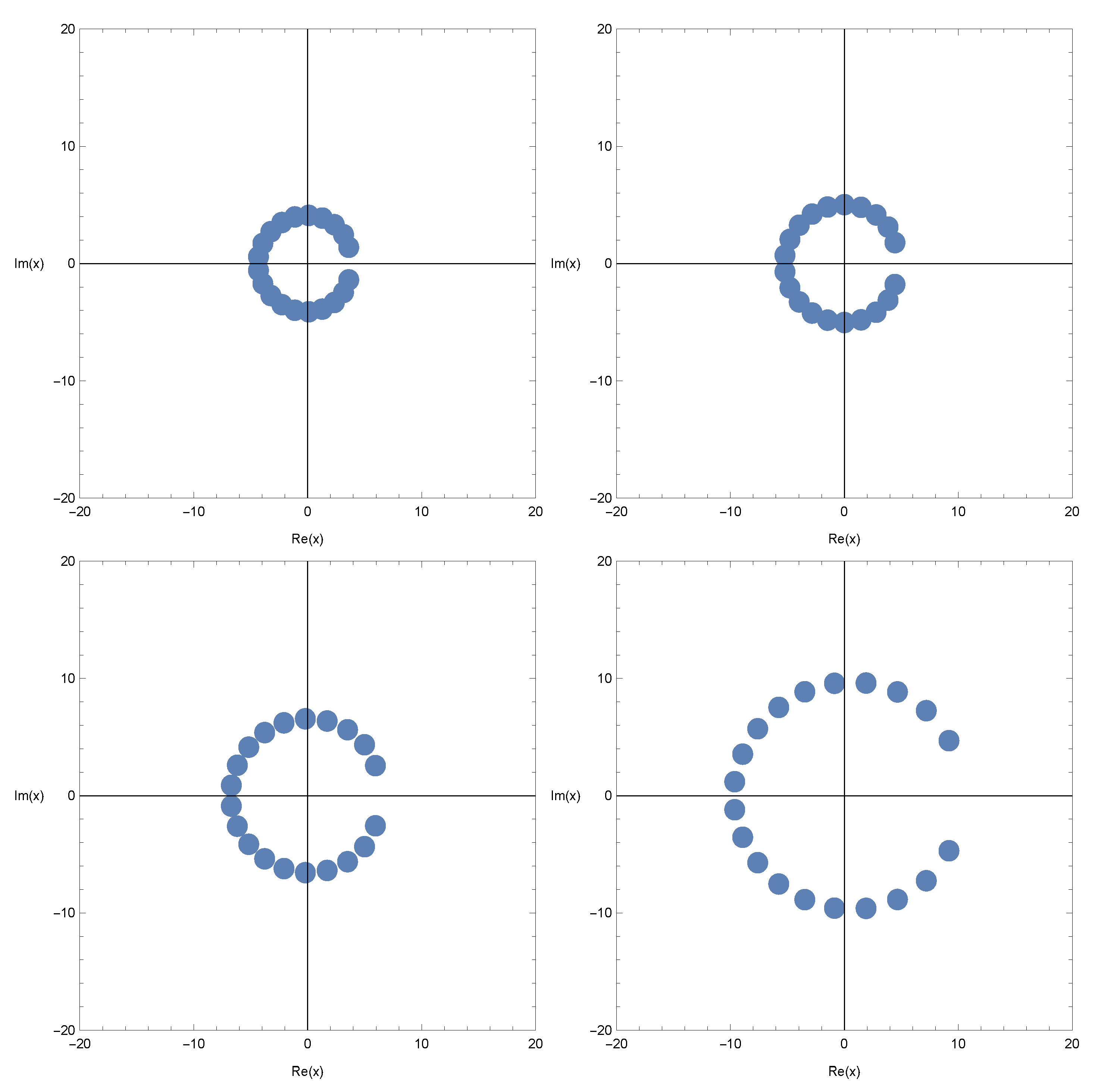
In this section, certain zeros of the q-Cosine Apostol-type Frobenius–Euler polynomials ${\mathbb{H}}_{n,q}^{(\alpha ,c)}(x,y;u;\lambda )$ and graphical representations are shown.

A few of them are as follows:

$$\begin{array}{l}{\mathbb{H}}_{0,q}^{(\alpha ,c)}(x,y;u;\lambda )={\left({\displaystyle \frac{-1+u}{u-\lambda }}\right)}^{\alpha },\hfill \\ {\mathbb{H}}_{1,q}^{(\alpha ,c)}(x,y;u;\lambda )=-{\displaystyle \frac{ux{\left(\frac{-1+u}{u-\lambda }\right)}^{\alpha }}{-u+\lambda }}+{\displaystyle \frac{x{\left(\frac{-1+u}{u-\lambda }\right)}^{\alpha }\lambda }{-u+\lambda }}-{\displaystyle \frac{\alpha {\left(\frac{-1+u}{u-\lambda }\right)}^{\alpha }\lambda }{-u+\lambda }},\hfill \\ {\mathbb{H}}_{2,q}^{(\alpha ,c)}(x,y;u;\lambda )={\displaystyle \frac{x^2{\left(\frac{-1+u}{u-\lambda }\right)}^{\alpha }}{(1-q)(1+q)}}-{\displaystyle \frac{q^2{x}^2{\left(\frac{-1+u}{u-\lambda }\right)}^{\alpha }}{(1-q)(1+q)}}-{\displaystyle \frac{y^2{\left(\frac{-1+u}{u-\lambda }\right)}^{\alpha }}{(1-q)(1+q)}}+{\displaystyle \frac{q^2{y}^2{\left(\frac{-1+u}{u-\lambda }\right)}^{\alpha }}{(1-q)(1+q)}}\hfill \\ +{\displaystyle \frac{u\alpha {\left(\frac{-1+u}{u-\lambda }\right)}^{\alpha }\lambda }{(1-q)(1+q){(-u+\lambda )}^2}}-{\displaystyle \frac{q^{2}u\alpha {\left(\frac{-1+u}{u-\lambda }\right)}^{\alpha }\lambda }{(1-q)(1+q){(-u+\lambda )}^2}}-{\displaystyle \frac{\alpha {\left(\frac{-1+u}{u-\lambda }\right)}^{\alpha }{\lambda }^2}{2(1-q)(1+q){(-u+\lambda )}^2}}\hfill \\ +{\displaystyle \frac{q\alpha {\left(\frac{-1+u}{u-\lambda }\right)}^{\alpha }{\lambda }^2}{2(1-q)(1+q){(-u+\lambda )}^2}}+{\displaystyle \frac{q^2\alpha {\left(\frac{-1+u}{u-\lambda }\right)}^{\alpha }{\lambda }^2}{2(1-q)(1+q){(-u+\lambda )}^2}}-{\displaystyle \frac{q^3\alpha {\left(\frac{-1+u}{u-\lambda }\right)}^{\alpha }{\lambda }^2}{2(1-q)(1+q){(-u+\lambda )}^2}}\hfill \\ +{\displaystyle \frac{{\alpha }^2{\left(\frac{-1+u}{u-\lambda }\right)}^{\alpha }{\lambda }^2}{2(1-q)(1+q){(-u+\lambda )}^2}}+{\displaystyle \frac{q{\alpha }^2{\left(\frac{-1+u}{u-\lambda }\right)}^{\alpha }{\lambda }^2}{2(1-q)(1+q){(-u+\lambda )}^2}}-{\displaystyle \frac{q^2{\alpha }^2{\left(\frac{-1+u}{u-\lambda }\right)}^{\alpha }{\lambda }^2}{2(1-q)(1+q){(-u+\lambda )}^2}}\hfill \\ -{\displaystyle \frac{q^3{\alpha }^2{\left(\frac{-1+u}{u-\lambda }\right)}^{\alpha }{\lambda }^2}{2(1-q)(1+q){(-u+\lambda )}^2}}-{\displaystyle \frac{x\alpha {\left(\frac{-1+u}{u-\lambda }\right)}^{\alpha }\lambda }{(1-q)(-u+\lambda )}}+{\displaystyle \frac{q^{2}x\alpha {\left(\frac{-1+u}{u-\lambda }\right)}^{\alpha }\lambda }{(1-q)(-u+\lambda )}}.\hfill \end{array}$$

We investigate the zeros of the q-Cosine Apostol-type Frobenius–Euler polynomials ${\mathbb{H}}_{n,q}^{(\alpha ,c)}(x,y;u;\lambda )$ by using a computer. We plot the zeros of the q-Cosine Apostol-type Frobenius–Euler polynomials ${\mathbb{H}}_{n,q}^{(\alpha ,c)}(x,y;u;\lambda )=0$ for $n=20$ (Figure 1).

In Figure 1 (top-left), we choose $\alpha =4,\lambda =2,u=3,$ and $q=\frac{1}{10},y=3$. In Figure 1 (top-right), we choose $\alpha =4,\lambda =2,u=3,$ and $q=\frac{3}{10},y=3$. In Figure 1 (bottom-left), we choose $\alpha =4,\lambda =2,u=3,$ and $q=\frac{5}{10},y=3$. In Figure 1 (bottom-right), we choose $\alpha =4,\lambda =2,u=3,$ and $q=\frac{7}{10},y=3$.

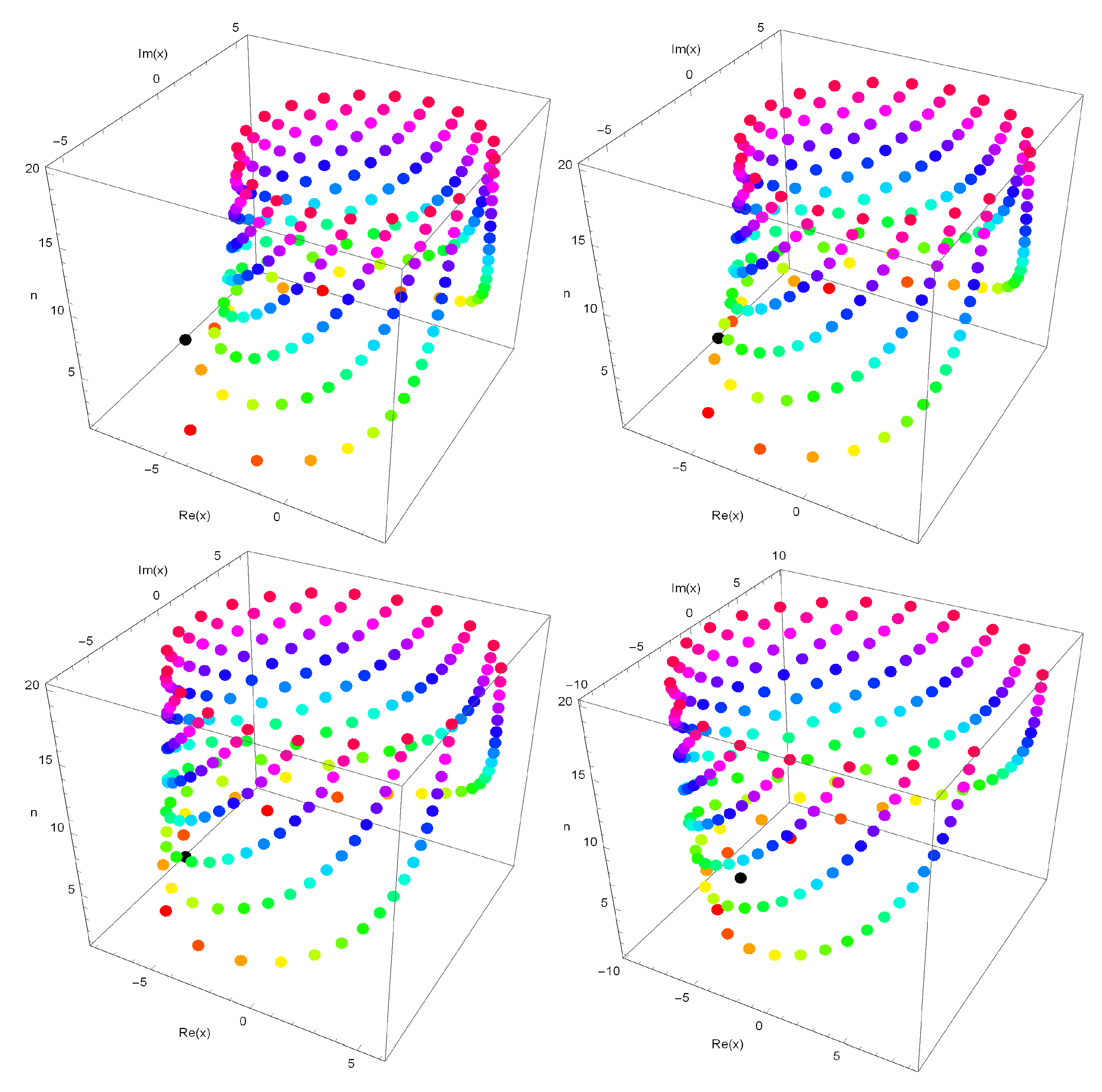
Stacks of zeros of the q-Cosine Apostol-type Frobenius–Euler polynomials ${\mathbb{H}}_{n,q}^{(\alpha ,c)}(x,y;u;\lambda )=0$ for $1\le n\le 20$, forming a 3D structure, are presented (Figure 2).

In Figure 2 (top-left), we choose $\alpha =4,\lambda =2,u=3,$ and $q=\frac{1}{10},y=3$. In Figure 2 (top-right), we choose $\alpha =4,\lambda =2,u=3,$ and $q=\frac{3}{10},y=3$. In Figure 2 (bottom-left), we choose $\alpha =4,\lambda =2,u=3,$ and $q=\frac{5}{10},y=3$. In Figure 2 (bottom-right), we choose $\alpha =4,\lambda =2,u=3,$ and $q=\frac{7}{10},y=3$.

Next, we calculated an approximate solution satisfying the q-Cosine Apostol-type Frobenius–Euler polynomials ${\mathbb{H}}_{n,q}^{(\alpha ,c)}(x,y;u;\lambda )=0$ for $q=\frac{1}{10}$. The results are provided in

Table 1. Approximate solutions of ${\mathbb{H}}_{n,q}^{(4,c)}(x,3;3;2)=0$.

Degree n	x
1	−8.0000
2	−4.4000 − 4.8621 i,    −4.4000 + 4.8621 i
3	−6.5429,    −1.1686 − 5.5743 i,    −1.1686 + 5.5743 i
4	−5.1586 − 2.9339 i,    −5.1586 + 2.9339 i,
	0.7146 − 5.2176 i,    0.7146 + 5.2176 i
5	−5.8344,    −3.3214 − 4.2756 i,    −3.3214 + 4.2756 i,
	1.7942 − 4.6626 i,    1.7942 + 4.6626 i
6	−5.1069 − 2.0266 i,    −5.1069 + 2.0266 i,    −1.7739 − 4.7670 i,
	−1.7739 + 4.7670 i,    2.4363 − 4.1334 i,    2.4363 + 4.1334 i
7	−5.4063,    −3.9859 − 3.2720 i,    −3.9859 + 3.2720 i,    −0.5893 − 4.8378 i,
	−0.5893 + 4.8378 i,    2.8338 − 3.6774 i,    2.8338 + 3.6774 i
8	−4.9566 − 1.5254 i,    −4.9566 + 1.5254 i,    −2.8747 − 3.9790 i,
	−2.8747 + 3.9790 i,    0.2982 − 4.7116 i,    0.2982 + 4.7116 i,
	3.0887 − 3.2950 i,    3.0887 + 3.2950 i
9	−5.1150,    −4.2106 − 2.6028 i,    −4.2106 + 2.6028 i,
	−1.8968 − 4.3377 i,    −1.8968 + 4.3377 i,    0.9638 − 4.5004 i,
	0.9638 + 4.5004 i,    3.2566 − 2.9754 i,    3.2566 + 2.9754 i

.

6. Symmetric Structure of Approximate Roots for q-Sine Apostol-Type Frobenius–Euler Polynomials and Their Application

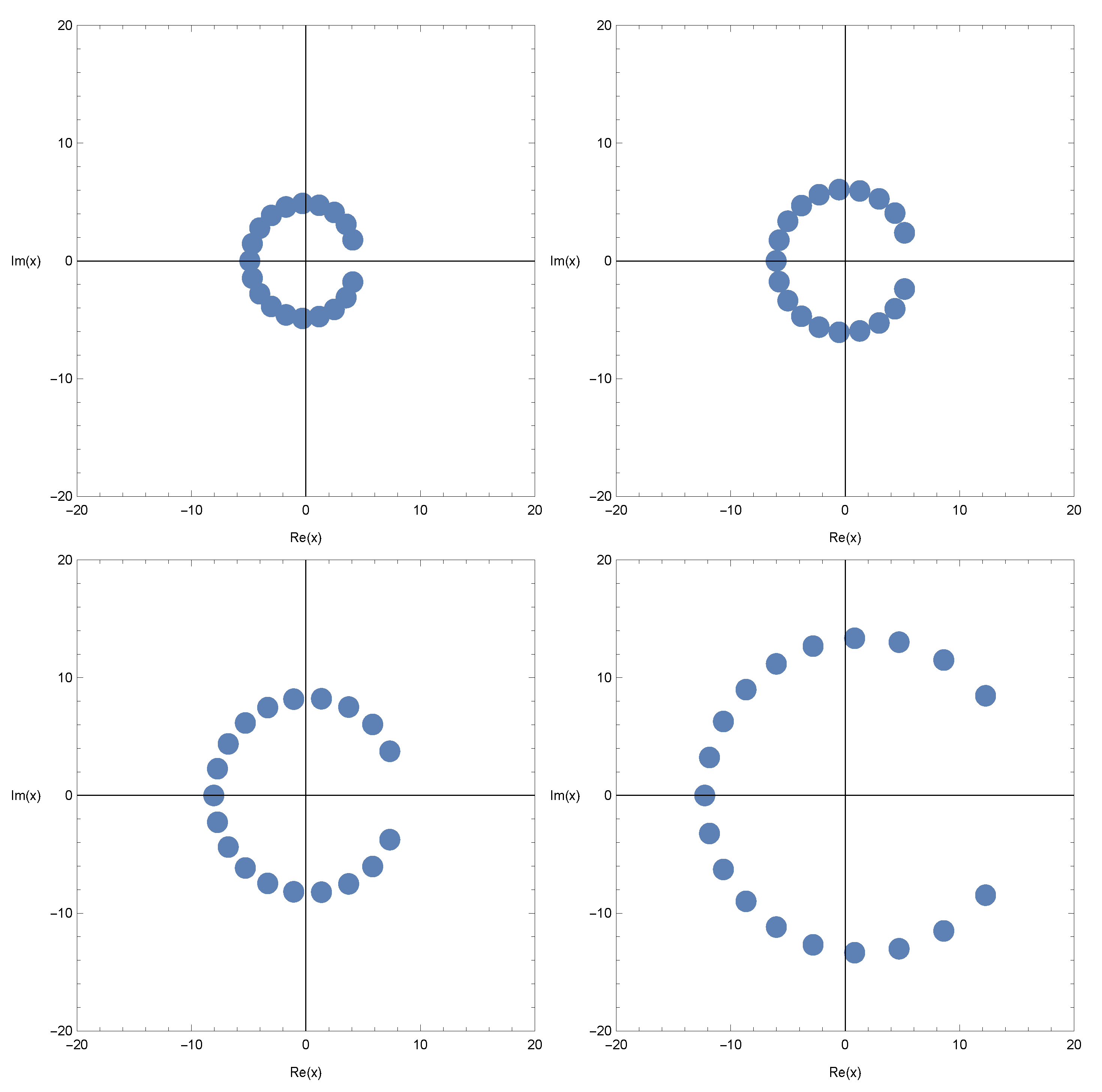
In this section, certain zeros of the q-Sine Apostol-type Frobenius–Euler polynomials ${\mathbb{H}}_{n,q}^{(\alpha ,s)}(x,y;u;\lambda )$ and beautiful graphical representations are shown.

A few of them are as follows:

$$\begin{array}{l}{\mathbb{H}}_{0,q}^{(\alpha ,s)}(x,y;u;\lambda )=0,\hfill \\ {\mathbb{H}}_{1,q}^{(\alpha ,s)}(x,y;u;\lambda )=y{\left({\displaystyle \frac{-1+u}{u-\lambda }}\right)}^{\alpha },\hfill \\ {\mathbb{H}}_{2,q}^{(\alpha ,s)}(x,y;u;\lambda )=-{\displaystyle \frac{uxy{\left(\frac{-1+u}{u-\lambda }\right)}^{\alpha }}{(1-q)(-u+\lambda )}}+{\displaystyle \frac{q^{2}uxy{\left(\frac{-1+u}{u-\lambda }\right)}^{\alpha }}{(1-q)(-u+\lambda )}}+{\displaystyle \frac{xy{\left(\frac{-1+u}{u-\lambda }\right)}^{\alpha }\lambda }{(1-q)(-u+\lambda )}}\hfill \\ -{\displaystyle \frac{q^{2}xy{\left(\frac{-1+u}{u-\lambda }\right)}^{\alpha }\lambda }{(1-q)(-u+\lambda )}}-{\displaystyle \frac{y\alpha {\left(\frac{-1+u}{u-\lambda }\right)}^{\alpha }\lambda }{(1-q)(-u+\lambda )}}+{\displaystyle \frac{q^{2}y\alpha {\left(\frac{-1+u}{u-\lambda }\right)}^{\alpha }\lambda }{(1-q)(-u+\lambda )}},\hfill \\ {\mathbb{H}}_{3,q}^{(\alpha ,s)}(x,y;u;\lambda )={\displaystyle \frac{x^{2}y{\left(\frac{-1+u}{u-\lambda }\right)}^{\alpha }}{{(1-q)}^2(1+q)}}-{\displaystyle \frac{q^2{x}^{2}y{\left(\frac{-1+u}{u-\lambda }\right)}^{\alpha }}{{(1-q)}^2(1+q)}}-{\displaystyle \frac{q^3{x}^{2}y{\left(\frac{-1+u}{u-\lambda }\right)}^{\alpha }}{{(1-q)}^2(1+q)}}\hfill \\ +{\displaystyle \frac{q^5{x}^{2}y{\left(\frac{-1+u}{u-\lambda }\right)}^{\alpha }}{{(1-q)}^2(1+q)}}-{\displaystyle \frac{q^3{y}^3{\left(\frac{-1+u}{u-\lambda }\right)}^{\alpha }}{{(1-q)}^2(1+q)(1+q+q^2)}}+{\displaystyle \frac{q^5{y}^3{\left(\frac{-1+u}{u-\lambda }\right)}^{\alpha }}{{(1-q)}^2(1+q)(1+q+q^2)}}\hfill \\ +{\displaystyle \frac{q^6{y}^3{\left(\frac{-1+u}{u-\lambda }\right)}^{\alpha }}{{(1-q)}^2(1+q)(1+q+q^2)}}-{\displaystyle \frac{q^8{y}^3{\left(\frac{-1+u}{u-\lambda }\right)}^{\alpha }}{{(1-q)}^2(1+q)(1+q+q^2)}}+{\displaystyle \frac{uy\alpha {\left(\frac{-1+u}{u-\lambda }\right)}^{\alpha }\lambda }{{(1-q)}^2(1+q){(-u+\lambda )}^2}}\hfill \\ -{\displaystyle \frac{q^{2}uy\alpha {\left(\frac{-1+u}{u-\lambda }\right)}^{\alpha }\lambda }{{(1-q)}^2(1+q){(-u+\lambda )}^2}}-{\displaystyle \frac{q^{3}uy\alpha {\left(\frac{-1+u}{u-\lambda }\right)}^{\alpha }\lambda }{{(1-q)}^2(1+q){(-u+\lambda )}^2}}+{\displaystyle \frac{q^{5}uy\alpha {\left(\frac{-1+u}{u-\lambda }\right)}^{\alpha }\lambda }{{(1-q)}^2(1+q){(-u+\lambda )}^2}}\hfill \\ -{\displaystyle \frac{y\alpha {\left(\frac{-1+u}{u-\lambda }\right)}^{\alpha }{\lambda }^2}{2{(1-q)}^2(1+q){(-u+\lambda )}^2}}+{\displaystyle \frac{qy\alpha {\left(\frac{-1+u}{u-\lambda }\right)}^{\alpha }{\lambda }^2}{2{(1-q)}^2(1+q){(-u+\lambda )}^2}}+{\displaystyle \frac{q^{2}y\alpha {\left(\frac{-1+u}{u-\lambda }\right)}^{\alpha }{\lambda }^2}{2{(1-q)}^2(1+q){(-u+\lambda )}^2}}\hfill \end{array}$$

$$\begin{array}{c}-{\displaystyle \frac{q^{4}y\alpha {\left(\frac{-1+u}{u-\lambda }\right)}^{\alpha }{\lambda }^2}{2{(1-q)}^2(1+q){(-u+\lambda )}^2}}-{\displaystyle \frac{q^{5}y\alpha {\left(\frac{-1+u}{u-\lambda }\right)}^{\alpha }{\lambda }^2}{2{(1-q)}^2(1+q){(-u+\lambda )}^2}}+{\displaystyle \frac{q^{6}y\alpha {\left(\frac{-1+u}{u-\lambda }\right)}^{\alpha }{\lambda }^2}{2{(1-q)}^2(1+q){(-u+\lambda )}^2}}\hfill \\ +{\displaystyle \frac{y{\alpha }^2{\left(\frac{-1+u}{u-\lambda }\right)}^{\alpha }{\lambda }^2}{2{(1-q)}^2(1+q){(-u+\lambda )}^2}}+{\displaystyle \frac{qy{\alpha }^2{\left(\frac{-1+u}{u-\lambda }\right)}^{\alpha }{\lambda }^2}{2{(1-q)}^2(1+q){(-u+\lambda )}^2}}-{\displaystyle \frac{q^{2}y{\alpha }^2{\left(\frac{-1+u}{u-\lambda }\right)}^{\alpha }{\lambda }^2}{2{(1-q)}^2(1+q){(-u+\lambda )}^2}}\hfill \\ -{\displaystyle \frac{q^{3}y{\alpha }^2{\left(\frac{-1+u}{u-\lambda }\right)}^{\alpha }{\lambda }^2}{{(1-q)}^2(1+q){(-u+\lambda )}^2}}-{\displaystyle \frac{q^{4}y{\alpha }^2{\left(\frac{-1+u}{u-\lambda }\right)}^{\alpha }{\lambda }^2}{2{(1-q)}^2(1+q){(-u+\lambda )}^2}}+{\displaystyle \frac{q^{5}y{\alpha }^2{\left(\frac{-1+u}{u-\lambda }\right)}^{\alpha }{\lambda }^2}{2{(1-q)}^2(1+q){(-u+\lambda )}^2}}\hfill \\ +{\displaystyle \frac{q^{6}y{\alpha }^2{\left(\frac{-1+u}{u-\lambda }\right)}^{\alpha }{\lambda }^2}{2{(1-q)}^2(1+q){(-u+\lambda )}^2}}-{\displaystyle \frac{xy\alpha {\left(\frac{-1+u}{u-\lambda }\right)}^{\alpha }\lambda }{{(1-q)}^2(-u+\lambda )}}+{\displaystyle \frac{q^{2}xy\alpha {\left(\frac{-1+u}{u-\lambda }\right)}^{\alpha }\lambda }{{(1-q)}^2(-u+\lambda )}}\hfill \\ +{\displaystyle \frac{q^{3}xy\alpha {\left(\frac{-1+u}{u-\lambda }\right)}^{\alpha }\lambda }{{(1-q)}^2(-u+\lambda )}}-{\displaystyle \frac{q^{5}xy\alpha {\left(\frac{-1+u}{u-\lambda }\right)}^{\alpha }\lambda }{{(1-q)}^2(-u+\lambda )}}\hfill \end{array}$$

In Figure 3 (top-left), we choose $\alpha =4,\lambda =2,u=3,$ and $q=\frac{2}{10},y=3$. In Figure 3 (top-right), we choose $\alpha =4,\lambda =2,u=3,$ and $q=\frac{4}{10},y=3$. In Figure 3 (bottom-left), we choose $\alpha =4,\lambda =2,u=3,$ and $q=\frac{6}{10},y=3$. In Figure 3 (bottom-right), we choose $\alpha =4,\lambda =2,u=3,$ and $q=\frac{8}{10},y=3$.

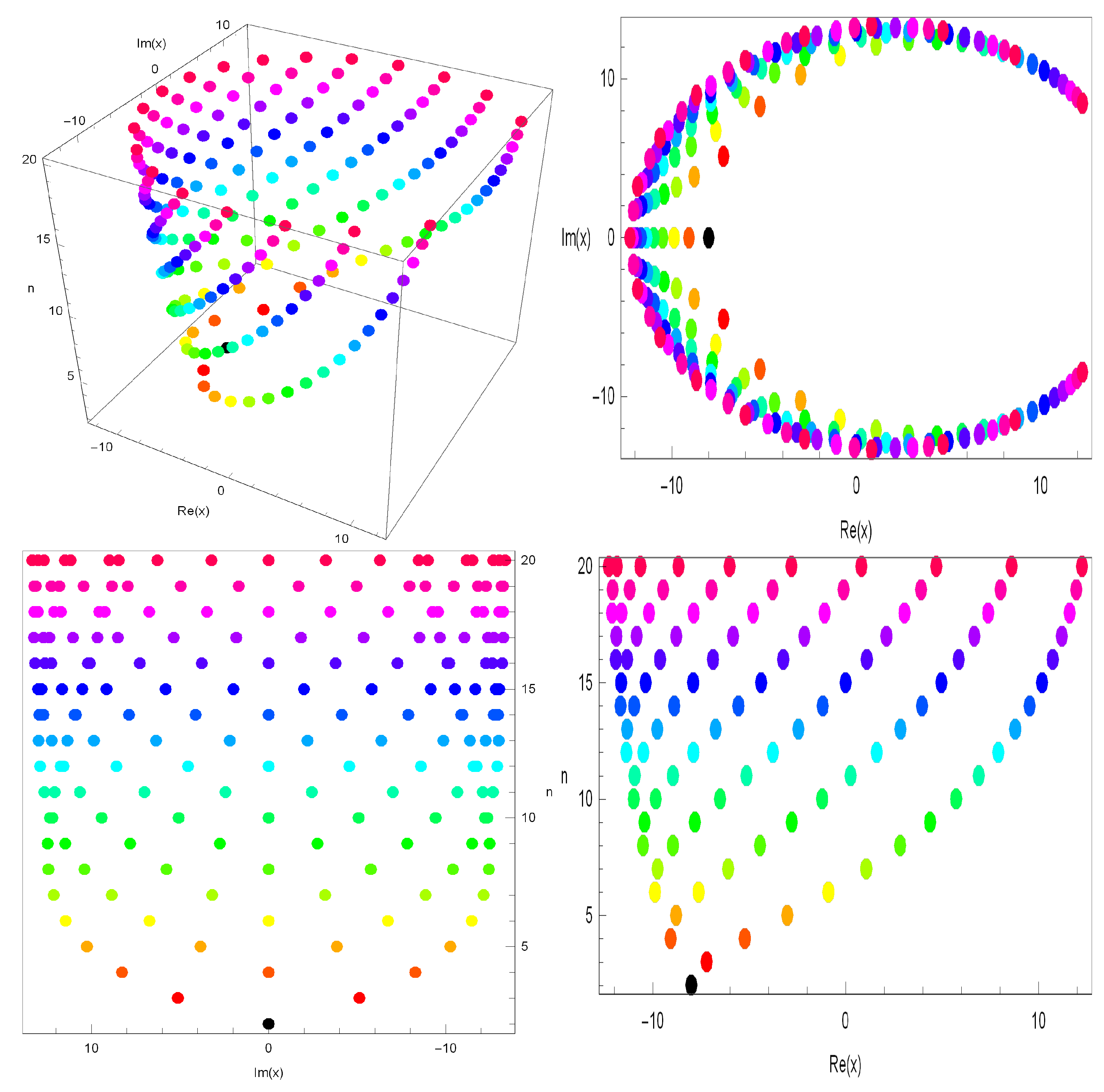
Stacks of zeros of the q-Sine Apostol-type Frobenius–Euler polynomials ${\mathbb{H}}_{n,q}^{(\alpha ,s)}(x,y;u;\lambda )=0$ for $2\le n\le 20$, forming a 3D structure, are presented (Figure 4).

In Figure 4 (top-left), we plot stacks of zeros of ${\mathbb{H}}_{n,q}^{(\alpha ,s)}(x,y;u;\lambda )=0$ for $2\le n\le 30$, $q=\frac{8}{10},\alpha =4,\lambda =2,u=3,y=3$. In Figure 4 (top-right), we draw x and y axes but no z axis in three dimensions. In Figure 4 (bottom-left), we draw y and z axes but no x axis in three dimensions. In Figure 4 (bottom-right), we draw x and z axes but no y axis in three dimensions.

Next, we calculated an approximate solution satisfying the q-Sine Apostol-type Frobenius–Euler polynomials ${\mathbb{H}}_{n,q}^{(\alpha ,s)}(x,y;u;\lambda )=0$ for $q={\displaystyle \frac{8}{10}}$. The results are given in

Table 2. Approximate solutions of ${\mathbb{H}}_{n,q}^{(4,s)}(x,3;3;2)=0$.

Degree n	x
2	−8.0000
3	−7.2000 − 5.1256 i,    −7.2000 + 5.1256 i
4	−9.0707,    −5.2247 − 8.2772 i,    −5.2247 + 8.2772 i
5	−8.7853 − 3.8486 i,    −8.7853 + 3.8486 i,
	−3.0227 − 10.2577 i,    −3.0227 + 10.2577 i
6	−9.8793,    −7.6190 − 6.7293 i,    −7.6190 + 6.7293 i,
	−0.8878 − 11.4618 i,    −0.8878 + 11.4618 i
7	−9.7452 − 3.1858 i,    −9.7452 + 3.1858 i,    −6.0868 − 8.8578 i,
	−6.0868 + 8.8578 i,    1.0748 − 12.1326 i,    1.0748 + 12.1326 i
8	−10.501,    −8.9527 − 5.7661 i,    −8.9527 + 5.7661i,    −4.4346 − 10.3981 i,
	−4.4346 + 10.3981 i,    2.8319 − 12.4327 i,    2.8319 + 12.4327 i
9	−10.4252 − 2.7531 i,    −10.4252 + 2.7531 i,    −7.8126 − 7.8189 i,
	−7.8126 + 7.8189 i,    −2.7879 − 11.4801 i,    −2.7879 + 11.4801 i,
	4.3811 − 12.4748 i,    4.3811 + 12.4748 i
10	−10.985,    −9.8411 − 5.0793 i,    −9.8411 + 5.0793 i,
	−6.5042 − 9.4234 i,    −6.5042 + 9.4234 i,    −1.2119 − 12.2069 i,
	−1.2119 + 12.2069 i,    5.7340 − 12.3389 i,    5.7340 + 12.3389 i
11	−10.9347 − 2.4373 i,    −10.9347 + 2.4373 i,    −8.9518 − 7.0112 i,
	−8.9518 + 7.0112 i,    −5.1343 − 10.6536 i,    −5.1343 + 10.6536 i,
	0.2605 − 12.6598 i,    0.2605 + 12.6598 i,    6.9078 − 12.0821 i,
	6.9078 + 12.0821 i

.

7. Conclusions

By making use of q-numbers and q-concepts, Jang et al. [2,4] defined q-Bernoulli polynomials and numbers, q-Genocchi polynomials and numbers and q-Euler polynomials and numbers and provided some new and interesting identities and formulae. With this viewpoint, several authors have introduced q-analogues of special numbers and polynomials and have investigated their properties. In this paper, by making use of the q-cosine polynomials and q-sine polynomials, we have considered a new class of q-analogues of Apostol-type Frobenius–Euler polynomials and have obtained new properties and identities. In addition, we have analysed the behaviour of q-integral and q-derivative representations. Additionally, we have checked the roots and graphical representations of these polynomials by making use of Mathematica software. This approach led us to consider different methods, and special cases of used variables of newly defined polynomial in the paper. In this viewpoint, we will try to continue working on newly considered polynomials in this line.

References

- Alam, N.; Khan, W.A.; Ryoo, C.S. A note on Bell-based Apostol-type Frobenius-Euler polynomials of complex variable with its certain applications. Mathematics 2022, 10, 2109. [Google Scholar] [CrossRef]
- Kang, J.Y.; Ryoo, C.S. Various structures of the roots and explicit properties of q-cosine Bernoulli polynomials and q-sine Bernoulli polynomials. Mathematics 2020, 8, 463. [Google Scholar] [CrossRef]
- Muhiuddin, G.; Khan, W.A.; Al-Kadi, D. Construction on the degenerate poly-Frobenius-Euler polynomials of complex variable. J. Funct. Spaces 2021, 2021, 3115424. [Google Scholar] [CrossRef]
- Ryoo, C.S.; Kang, J.Y. Explicit properties of q-Cosine and q-Sine Euler polynomials containing symmetric structures. Symmetry 2020, 12, 1247. [Google Scholar] [CrossRef]
- Kim, D.S.; Kim, T.; Lee, H. A Note on Degenerate Euler and Bernoulli Polynomials of Complex Variable. Symmetry 2019, 11, 1168. [Google Scholar] [CrossRef]
- Kim, T.; Ryoo, C.S. Some Identities for Euler and Bernoulli Polynomials and Their Zeros. Axioms 2018, 7, 56. [Google Scholar] [CrossRef]
- Masjed-Jamei, M.; Beyki, M.R.; Koepf, W. A New Type of Euler Polynomials and Numbers. Mediterr. J. Math. 2018, 15, 138. [Google Scholar] [CrossRef]
- Srivastava, H.M.; Masjed-Jamei, M.; Beyki, M.R. A Parametric Type of the Apostol-Bernoulli, Apostol-Euler and Apostol-Genocchi Polynomials. Appl. Math. Inf. Sci. 2018, 12, 907–916. [Google Scholar] [CrossRef]
- Arjika, S. On q2-Trigonometric functions and their q2-Fourier transform. J. Math. Syst. Sci. 2019, 9, 130–135. [Google Scholar] [CrossRef]
- Koekoek, R.; Lesky, P.A.; Swarttouw, R.F. Hypergeometric Orthogonal Polynomials and Their q-Analogues; Springer: Berlin/Heidelberg, Germany, 2010. [Google Scholar]
- Kurt, B. A note on the Apostol type q-Frobenius-Euler polynomials and generalizations of the Srivastava-Pinter addition theorems. Filomat 2016, 30, 65–72. [Google Scholar] [CrossRef]
- Kang, J.Y.; Khan, W.A. A new class of q-Hermite based Apostol type Frobenius Genocchi polynomials. Commun. Korean Math. Soc. 2020, 35, 759–771. [Google Scholar]
- Kim, T.; Kim, D.S.; Jang, L.C.; Kim, H.-Y. On type 2 degenerate Bernoulli and Euler polynomials of complex variable. Adv. Differ. Equ. 2019, 2019, 490. [Google Scholar] [CrossRef]
- Kac, V.; Cheung, P. Quantum Calculus; Springer: New York, NY, USA, 2001. [Google Scholar]
- Mahmudov, N.I. q-analogues of the Bernoulli and Genocchi polynomials and the Srivastava-Pinter addition theorems. Discrete Dyn. Nat. Soc. 2012, 2012, 169348. [Google Scholar] [CrossRef]
- Mahmudov, N.I. On a class of q-Bernoulli and q-Euler polynomials. Adv. Differ. Equ. 2013, 2013, 108. [Google Scholar] [CrossRef]