
Denoising in Representation Space via Data-Dependent Regularization for Better Representation

1
School of Computer Science and Engineering, Northeastern University, Shenyang 110169, China
2
School of Automation and Electrical Engineering, Shenyang Ligong University, Shenyang 110159, China
*
Author to whom correspondence should be addressed.
Mathematics 2023, 11(10), 2327; https://doi.org/10.3390/math11102327
Submission received: 11 April 2023
/
Revised: 11 May 2023
/
Accepted: 15 May 2023
/
Published: 16 May 2023
(This article belongs to the Special Issue Advances in Computer Vision and Machine Learning)
Abstract
:Despite the success of deep learning models, it remains challenging for the over-parameterized model to learn good representation under small-sample-size settings. In this paper, motivated by previous work on out-of-distribution (OoD) generalization, we study the representation learning problem from an OoD perspective to identify the fundamental factors affecting representation quality. We formulate a notion of “out-of-feature subspace (OoFS) noise” for the first time, and we link the OoFS noise in the feature extractor to the OoD performance of the model by proving two theorems that demonstrate that reducing OoFS noise in the feature extractor is beneficial in achieving better representation. Moreover, we identify two causes of OoFS noise and prove that the OoFS noise induced by random initialization can be filtered out via L2 regularization. Finally, we propose a novel data-dependent regularizer that acts on the weights of the fully connected layer to reduce noise in the representations, thus implicitly forcing the feature extractor to focus on informative features and to rely less on noise via back-propagation. Experiments on synthetic datasets show that our method can learn hard-to-learn features; can filter out noise effectively; and outperforms GD, AdaGrad, and KFAC. Furthermore, experiments on the benchmark datasets show that our method achieves the best performance for three tasks among four.
MSC:
68T071. Introduction
Although deep learning has made great progress in recent years, many questions remain to be answered, such as why some models can generalize well despite the fact that they are over-parameterized [1], why adversarial examples exist [2], why representations learned by models are difficult to transfer across various domains [3], and why handling out-of-distribution (OoD) samples is difficult for models [4]. Thus, the mechanisms underlying deep learning still require further exploration. In particular, in the small-sample-size regime, models are more prone to overfitting. In order to achieve better generalization, careful capacity control is needed via methods such as regularization.
We consider deep neural networks (DNNs) to be a functional composition of the following form: , where denotes a feature extractor that maps the input into an internal representation space and then a linear classifier is used to predict the class label. We can infer that, in a small-sample-size setting, good generalization performance depends more on good representations. However, most research on generalization [5,6] is based on an assumption that the training and test samples are from the same distribution, and many studies on representation learning [7,8] are based on this assumption; however, the theoretical bounds, methods, and experimental studies based on such an assumption cannot guarantee that the model learns good representations, especially in situations where the sample size is small. Specifically, biases of stochastic gradient descent (SGD) and cross-entropy loss might maximize the margins of the training set [9], which seems beneficial for generalization with sufficient data and under the i.i.d. assumption. However, for more complex and difficult applications, such as domain generalization (DG) [3,10,11], open set recognition (OSR) [4,12], or OOD generalization [13,14], or in situations with insufficient training samples [15], these representations may not be sufficient.
Inspired by the questions and research in fields such as OSR and OoD generalization, here, we study a representation learning problem under a small-sample-size setting via a broader perspective, i.e., we take both in-distribution generalization and OoD generalization performance into consideration to learn better representations. This paper is based on the following assumption: A good representation should achieve good in-distribution performance, without compromising OoD performance. Therefore, we argue that good OoD performance may be an indicator of good representation.
The first questions we ask are as follows: What is a good representation? Or, what makes a good feature extractor? However, these questions are not easy to answer; hence, we ask the following questions instead:
What makes a not-so-good feature extractor? Why does the model learn a poor ? What is the impact of a poor (noisy) ? Additionally, how can we encourage the model to learn a better ?
In this paper, we try to explore these questions from a signal-processing perspective. Specifically, we formulate the notion “out-of-feature subspace (OoFS) noise” for a single-hidden-layer neural network with the aid of a feature dictionary and employ this notion to characterize “what makes a poor ”, i.e., when contains a lot of “OoFS noise”. We identify two causes of such a noisy and study the impact of OoFS noise in on random OoD samples. Furthermore, we propose a data-dependent regularizer that acts on the weights of the fully connected layer and rely on the back-propagation scheme to force to focus more on signal and to rely less on noise.
The way we consider the representation learning problem is similar to the hypothesis in [16], in which the author tried to explain the success of dropout training as such: dropout achieves gains much like a marathon runner who practices at altitudes, i.e., once a model learns to perform well on corrupted training samples, it performs very well on an uncorrupted test set. In our study, we seek to improve the performance of representation learning by forcing the model to solve a more difficult problem. Intuitively, we argue that the OoFS noise in acts as an indicator of the quality of and a noisy hurts generalization. Under this assumption, we require the model to seek a solution that contains less OoFS noise and view this kind of solution as a better solution that may be beneficial for generalization potentially.
Our contributions are as follows:
- (1)
- Using a data model based on a feature dictionary, we propose the notion of OoFS noise and argue that OoFS noise is a factor that leads to poor representation and hurts generalization. To our knowledge, we are the first to propose this notion. Additionally, we theoretically study OoFS noise in the feature extractor of a single-hidden-layer neural network and prove two theorems to (probabilistically) bound the output of a random OoD test point. Moreover, we identify two sources of OoFS noise and prove that OoFS noise due to random initialization can be filtered out via L2 regularization (Section 3).
- (2)
- Because both the noises in the data and the model are embedded in the representations, we propose a novel approach to regularizing the weights of the fully connected layer in a data-dependent way, which aims to reduce noise in the representation space and implicitly force the feature extractor to focus more on informative features instead of relying on noise (Section 4).
- (3)
- We propose a new method to examine the behavior and to evaluate the performance of a learning algorithm via a simple task. Specifically, we disentangle the model’s performance into two distinct aspects and, thus, inspect each aspect individually (Section 5.1).
The rest of the paper is structured as follows: In Section 2, we review related work. In Section 3, we consider a data model based on a feature dictionary and a single-hidden-layer convolutional neural network and present some novel notions under this setting; then, we study the impact of OoFS noise in the feature extractor on OoD test samples theoretically. Based on this understanding, in Section 4, we focus on the signals and noise in the representation space of DNNs and propose a data-dependent regularization method that acts on the weights of the fully connected layer. In Section 5, we present the experimental results on synthetic and benchmark datasets. Finally, we provide the conclusions in Section 6.
2. Related Work
Two lines of previous work are related to our work. The first focuses on the feature learning process. Among them, the authors of [17] studied a two-layer ReLU network and proved that the feature learned by each neuron contains a non-robust dense mixture of the features, and these mixtures are one of the causes of adversarial examples. The authors suggested that adversarial training is actually a feature purification process. The authors of [18] designed a multi-view data model and proposed that, when the dataset has this multi-view structure, a network trained with cross-entropy loss via gradient descent (GD) quickly picks up a subset of features for each label such that the majority of the training examples are classified correctly; then, the model memorizes the remaining single-view data without learning other informative features. The authors of [19] studied how momentum improves generalization and proved that a model trained via GD initially only learns the large-margin data and then memorizes the remaining small-margin data. In contrast, a model trained via GD with momentum accumulates large historical gradients and, thus, can keep learning features and memorizing less noise. The authors of [20] considered a linear DNN and proposed that the learning dynamics is closely related to the singular value decomposition (SVD) of the input–output correlation matrix and that modes with stronger explanatory power, as quantified by the singular value, are learned more quickly. The authors of [21] studied the learning dynamics of a single-hidden-layer ReLU neural network and showed that input norm and the features’ frequency in the dataset lead to distinct convergence speeds, which might be related to the generalization performance of the model. They identified a phenomenon named gradient starvation, where the most frequent features in a dataset prevent the learning of other less frequent but equally informative features. The authors of [22] defined gradient starvation via the SVD of the neural tangent random feature (NTRF) matrix to characterize the phenomenon in which the model minimizes cross-entropy loss by capturing only a subset of features and fails to discover other predictive features. The authors also provided a theoretical explanation for this feature imbalance. The authors of [23,24,25,26] studied the simplicity bias in DNNs, i.e., the model can rely on the simplest features and remains invariant to other predictive complex features. The authors of [27] split the Jacobian spectrum into “information” and “nuisance” spaces associated with large and small singular values and showed that the generalization capability of the model is controlled by how well the label vector is aligned with the information space. Many studies have tried to improve the feature learning process from an optimization perspective. The authors of [28] proposed the AdaGrad optimization algorithm; they used historical information of gradients to enable the model to better learn those highly predictive but rare features that are hard to learn. The authors of [29] proved that natural gradient descent (NGD) [30] outperforms GD in the misaligned setting, whereas GD has an advantage when the signal is aligned. The authors showed that a preconditioned update that interpolates between GD and NGD can be performed to obtain an optimal empirical risk.
The second line related to our work is the capacity control based on explicit or implicit regularization. Among them, weight decay is widely used, and it has been proven that, for SGD, weight decay is equivalent to L2 regularization with a specific regularization coefficient [31]. It is well known that, for underdetermined least square problems, GD converges to the minimum Euclidean norm solution, and for logistic regression problems, GD converges to the L2 maximum margin separator [9]. However, the bias towards the minimum Euclidean norm or the max-margin solution is not necessarily optimal. The authors of [32] proposed that this bias is one of the failure modes of OoD generalization. The authors of [33] proved that max-margin bias induces bias towards non-robust networks. The authors of [34,35] suggested that capacity control based on L2 norm is not necessarily well linked to generalization performance. The authors of [36] studied a linear predictor for the ridgeless least square problem and provided a bias-variance decomposition of the prediction risk, where the bias term was expressed by a matrix norm with respect to the covariance of the data; this hints at the generalization being related to the geometry of the data. The authors of [37] identified a regularization effect induced by a dynamical alignment of the neural tangent kernel (NTK) along a small number of task-relevant directions and showed that meaningful norm-based capacity control is closely related to the geometry of features and labels. The authors of [38] proved that, for matrix completion, dropout induces a data-dependent regularizer that directly controls the complexity of the underlying class of DNNs. The authors of [39] showed that dropout can be viewed as a low-rank regularizer with data-dependent singular-value thresholding. The authors of [40] considered a single-hidden-layer linear neural network, and showed that, as a regularizer, dropout is closely related to path regularization. The authors of [41] showed that dropout can be viewed as a form of adaptive regularization and is related to AdaGrad, and that the dropout regularizer is first-order equivalent to an L2 regularizer applied after scaling the features using an estimate of the inverse diagonal Fisher information matrix. The authors of [42] considered the cross-domain generalization problem and proposed a method that iteratively challenges the dominant features to force the network to activate remaining features. The authors of [43] proposed a Jacobian regularizer to increase the margins of a model under input perturbations. Moreover, many studies regularized activations in the latent space to improve generalization. The authors of [44] proposed a regularizer to encourage diverse representations by minimizing the cross-covariance of hidden activations. The authors of [45] proposed performing class-wise regularization to minimize the pairwise distances between representations of a class. Finally, the authors of [15] proposed a topological regularizer that acts on the samples drawn from the probability measure of the representation space and proved the existence of a mass concentration effect, which is beneficial for generalization.
3. Theoretical Analysis of the Noise in Hidden Neurons
When training and test data are sampled from the same underlying distribution and when the amount of data is sufficient, things are, in some sense, controllable most of the time; a noisy model may still achieve good performance because neurons can cooperate to cancel noise for the in-distribution input. However, things can change wildly under more complex settings, such as, for OoD samples, the model extrapolating arbitrarily and the noise hurting generalization in an unpredictable manner. In small-sample-size learning, we face a similar problem. In this paper, we argue that to achieve good performance when data are insufficient, understanding the signal and noise in the model is crucial, and this knowledge can be incorporated into the learning algorithm as a means of capacity control.
Therefore, in this section, we focus on the signal and noise in the model theoretically; in particular, we consider the noise in the OoF subspace (we refer to it as “OoFS noise” for simplicity in the following) in the hidden neurons. We first introduce the data model and the neural network model; then, we present some notions and theoretical analyses. Specifically, we bound the impact of the OoFS noise in the model on random Gaussian OoD test samples using Theorem 1 and Theorem 2, thus linking OoFS noise to generalization. We also identify two causes of OoFS noise in the model; the first cause is due to the noise in the training data, which is memorized by the model, and this memorization can be reduced via a better feature learning process; the second cause is due to the noise induced by random initialization, and it can be reduced via proper capacity control methods, such as L2 regularization, as formulated in Theorem 3.
3.1. Data Distribution, Model, and Definitions
To understand the learned features from a signal-processing perspective, in particular, to understand the signal and noise in neurons, we need to consider the signal and noise in the data first. In this subsection, we adopt a data model based on a feature dictionary [17] to formulate some notions.
Let be a feature dictionary. There are features in the dictionary, and each feature is a d-dimensional vector. We denote the i-th feature by , i.e., the i-th column of . For simplicity, we adopt the same assumption as in [17]; let and be a unitary matrix, i.e., . Assume that the training data are generated based on this dictionary. We denote the training set by , where is the input, is the label, and n is the number of training samples. Furthermore, assume that each input is composed of P patches; let it be .
Take a binary classification task as an illustrative example: Let . Assume that the points in Class 1 contain features and and that the points in Class 2 contain features and . Figure 1 shows a sample from Class 1. We refer to ~ as the ground-truth features and denote the submatrix composed of the first four columns of by .
Under the above setting, we can decompose the d-dimensional space spanned by the columns of the feature dictionary into two subspaces: (1) One is the feature subspace (FS; note that this is not the feature space in the DNN literature) relevant to the task, denoted by . We view it as the signal subspace. In this example, it is the subspace spanned by . (2) The other is the out-of-feature subspace (OoF subspace, OoFS). The other features in the dictionary are not relevant to the task as they span the OoF subspace. This subspace is the orthogonal complement of the feature subspace; we denote it by and view it as the noise subspace (with respect to the current task).
Next, considering the support of the data distribution, the feature subspace can be further divided into two subsets: (1) If there is no OoFS noise in the data, then the support of the data distribution is generally a bounded subset of the feature subspace . We call it the “data support in the feature subspace”, denoted by . When there is OoFS noise in the data, corresponds to the projection of the support onto the feature subspace. (2) The complementary set of (CoS) in the feature subspace is denoted by .
Figure 2 shows the division of the -dimensional space. From this viewpoint, we argue that a good model should focus on the signal in the feature subspace instead of relying on the OoFS noise, and the learning algorithm should filter out the OoFS noise in the model as much as possible.
In the following, to keep the theoretical analysis simple, we follow the setting in [19] and consider a special case, i.e., there is only one feature relevant to the task; we denote it by for simplicity. The data distribution is determined as follows:
- (1)
- Uniformly sample the label from {−1, 1}.
- (2)
- Let , where each patch .
- (3)
- Signal patch: choose one signal patch such that , where , , and .
- (4)
- is distributed as with probability , and otherwise, where corresponds to the majority of the samples that have a large margin and corresponds to the minority of samples that have a small margin.
- (5)
- Noisy patches: , for .
Now that we have defined the data distribution and differentiated the signal and noise in the data, we are in a place to study the signal and noise in the model. Consider a single-hidden-layer neural network as in [19]:
where m is the number of hidden neurons, and the weights of the first layer are denoted by . We denote the r-th row of by , corresponding to the incoming weights of the hidden neuron r. We refer to as the feature (i.e., the hidden weight) of the r-th neuron. The weights of the second layer are fixed to .
Then, we can characterize and measure signals and OoFS noise in the neurons during training. Let , , , , and the hidden weight of the r-th neuron at time t be denoted by . Let represent the gradient of with respect to . Let be the projection of onto the ground-truth feature , which can be viewed as the signal contained in the hidden weight of the r-th neuron. Let be the projection of onto the OoF subspace, which can be viewed as the OoFS noise contained in the hidden weight of the r-th neuron. Let be the maximum signal, where . Let for .
The objective is . Let and for . Moreover, we use , , and to hide the logarithmic dependency on d. The parameters are chosen as in [19]: , , ,, , , , , and . Finally, is used to describe when the sigmoid term is small such that
3.2. The Impact of OoFS Noise in the Model
In this subsection, assume that there is OoFS noise in the training data. According to the feature learning process described in [18,19], the network quickly picks up the dominant features that appear in the large-margin data to decrease their training loss. Once the large-margin data are classified correctly, the gradient terms stemming from them become negligible. Consequently, the gradient becomes a sum of the gradients of the small-margin data. Thus, the model memorizes the noise in these samples to decrease the training loss. In short, the model memorizes noise to fit small-margin samples.
According to [19], the weights learned via GD and GD with momentum (GD+M) satisfy the following for :
- (1)
- For GD, and for all .
- (2)
- For GD+M, at least one of , and for all .
Based on these results, and noting that corresponds to the OoFS noise in the hidden weight of the r-th neuron, we prove the following Theorems 1 and 2. In Theorem 1, we turn off the signal patch and bound the model’s output for a random OoD test sample, in which each patch is sampled from a Gaussian distribution on the OoF subspace.
Theorem 1.
For the above-mentioned single-hidden-layer model, assume that we run GD/GD+M for T iterations with the above parameterization and that is a random test sample that satisfies for all ; then, we have the following:
- (1)
- For GD and arbitrary , . Specifically, setting , we have: .
- (2)
- For GD and GD+M, we have: . Specifically, for GD, we have: , and for GD+M, we have: .
Proof.
According to Equations (1) and (3), the output of the model for the test sample is:
- (1)
- For GD, since holds for all , then, according to Lemma K.12 in [19], for , we have:
- (2)
- We know that ; then, by Lemma K.13 in [19], we have: is -subGaussian.>
Using Lemma K.2 in [19], we know that is -subGaussian. Applying Lemma K.2 again, we obtain that is -subGaussian.
Then, we use Lemma K.3 in [19] to upper bound this subGaussian random variable and obtain:
Thus,
For GD, since , and , we have:
For GD+M, we have: ; then, we have:
□
Theorem 1 shows that because the OoFS noise terms in the hidden weight of the neurons may have non-zero correlations with a test sample from the OoF subspace, the output of the model is non-zero. From (2) in Theorem 1, we see that as increases, the upper bound of becomes looser, which indicates a larger probability of the output exceeding a pre-determined value. This is consistent with our intuition that when the noise level in the data increases, the noise in the output also increases. Furthermore, Theorem 1 demonstrates that when increases, the upper bound becomes looser, which means that when the noise in the neurons increases, the noise in the output increases consequently. Therefore, increasing the noise in the data or increasing the noise in the model results in a noisier output, corresponding to a larger probability of misclassifying the OoD point as an in-distribution point.
In Theorem 2, we turn on the signal patch, i.e., assume the OoD test sample has a non-zero correlation with the feature in some patch and bound the model’s output for such a test sample.
Theorem 2.
For the above-mentioned single-hidden-layer model, assume that we run GD/GD+M for T iterations with the above parameterization and assume that is a random OoD test sample that contains some feature noise, i.e., for some , let and let for simplicity, and for all , let ; then, we have the following:
- (1)
- For GD, ;
- (2)
- For GD+M, ;
- (3)
- For GD, ;
- (4)
- For GD+M, .
Proof.
(1) First, let us consider the upper bound of , we have:
(i) For GD, according to Induction hypothesis D.2 [19], we have: ; then,
Since is -subGaussian; then, according to Lemma K.3 in [19], we have:
Then, we have:
Therefore,
Then, we have:
Combined with Equation (11), we obtain:
Since , we have:
(ii) For GD+M, according to Induction hypothesis D.5 in [19], ; then, combined with Equation (10), we have:
Since , combined with Equation (12), we have:
Thus,
Then, we have:
Consequently, we have:
i.e.,
(2) Then, we consider the lower bound, we have:
(i) For GD, we have:
According to Lemma K.12 in [19], we know that:
Thus, we have:
Combined with Equation (25), we have:
Setting , we obtain:
(ii) For GD+M, according to Lemma 6.3 in [19], we have: , and thus, ; then, combined with Equation (24), we have:
Using Lemma K.3 in [19], we have:
Then, we have:
Thus, we obtain:
Combined with Equation (30), we have:
We note that ; then, we obtain:
□
Theorem 2 shows that for an OoD sample that has a non-zero correlation with the feature, we have the following: (1) As (i.e., the correlation with the feature) increases, the output increases and the upper bound of the output becomes looser, which is consistent with our intuition. (2) As decreases, the upper bound of the output becomes looser, which means that when the signal in the neurons increases, the output increases. (3) As increases, i.e., the noise in the data increases, the bound becomes looser, which means that we are less confident that the output will be smaller than a pre-determined value. (4) As increases, i.e., the OoFS noise in the neurons increases, the bound becomes looser, again, and we are less confident that the output will be smaller than a pre-determined value.
In the above, we discuss the first cause of OoFS noise in the model, i.e., the model memorizes the noise in the small-margin data during training to decrease their training losses. In order to reduce this kind of noise, we may employ methods that favor hard-to-learn features [22,28,42], and we may also resort to regularization methods, such as those in [41].
3.3. The OoFS Noise in the Model Induced by Random Initialization
In this subsection, we use the same model and data distribution as in Section 3.2, except that we assume that there is no OoFS noise in the data (i.e., the noise patches are all zero); then, we can identify another cause of OoFS noise in the model, i.e., the noise induced by random initialization. In this setting, for the r-th neuron, assume that we have for at least one k, where , i.e., is one of the features that are irrelevant to the task (remember that is the only feature relevant to the task).
Take the linear model as an illustrative example when using GD and squared loss without regularization; because the gradients of the loss are always constrained to the fixed subspace spanned by the data [46], the weight are confined to the low-dimensional affine manifold . If there is no OoFS noise in the data, then we have: ; hence, for all and . This demonstrates that if we do not impose any capacity control, the OoFS noise remains in the model; although it is irrelevant to the task, the model has no incentive to filter them out.
Since forms the orthogonal basis of the OoF subspace, let , where and ; then, characterizes the OoFS noise in the hidden neurons induced by random initialization. For GD and GD+M, we can write , since ; then, we have: , i.e., , and thus, . According to Theorems 1 and 2, we know that reducing is beneficial for OoD samples; in the following Theorem 3, we prove that L2 regularization can filter out the OoFS noise in the model, thus reducing .
Theorem 3.
Assume that we run GD on the above-mentioned single-hidden-layer model with the above parameterization. Assume that , , , and the training objective is . Let , where and ; then, we have: for all r and k, where is the learning rate and when , .
In order to ensure for some , should satisfy . To ensure for all r and k, T should satisfy . Moreover, to ensure , we may require , which means
Proof.
Via gradient update, for , we have:
where .
According to Lemma E.1 in [19], we know the following:
Since for , the gradients are constrained to the fixed one-dimensional subspace spanned by ; thus, , and we obtain the following:
To satisfy , we should have:
Thus, we have: . In practice, we know that is small; so, we can use the Taylor expansion for . Using , we have
□
From Theorem 3, we know that weight decay or L2 regularization can be used to filter out the OoFS noise in the model, but there are also trade-offs: First, the convergence is slow; we need to train for a long time to reduce the noise below a pre-defined threshold. Second, weight decay imposes the same level of penalty for all the parameters in the model regardless of the geometry of the data. Third, setting the weight decay to a large value hurts generalization. Therefore, we need other capacity control schemes to filter out the OoFS noise.
Based on the above understanding, we can infer that the OoD generalization performance is related to both the test distribution and the model’s properties. First, we can evaluate the performance of the model from two aspects:
- (1)
- The performance in the feature subspace, which further depends on two factors: (i) Does the model learn all the informative features, i.e., does the model learn the basis of and the relative strength of the learned features, i.e., the signal strength , in the hidden neurons? (ii) How does the model explain the data in ? Different algorithms have different biases and provide different explanations;
- (2)
- The performance in the OoF subspace, which is determined by the OoFS noise in the model.
Second, considering the distribution of the test data, we can evaluate the performance by sampling test data from the feature subspace and the OoF subspace individually and by obtaining the model’s responses to them, as we show in Section 5.1.
Therefore, we can evaluate algorithms under this simple setting to understand their behaviors and to evaluate their performance from the above two distinct aspects, which may help us to improve existing algorithms or to develop new algorithms.
4. From Neurons to Representations—Data-Dependent Regularization for the Fully Connected Layer
In Section 3, we study the impact of the OoFS noise in the model on the OoD test samples under a simplified setting, i.e., a single-hidden-layer neural network and a data model based on a feature dictionary. Although things are more complicated for natural datasets and DNNs, we can still gather some insights from the above analysis. First, in order to learn a good representation, we should suppress the OoFS noise in the feature extractor. Although we cannot directly measure OoFS noise anymore for DNNs, from Theorems 1 and 2, we can see that both the noise in the data and the noise in the model are embedded in the output; thus, in order to reduce the noise in the feature extractor, we focus on the representations. However, signal and noise in the representations are still difficult to define and measure; hence, inspired by [20,22,37] in which modes with stronger explanatory power can be quantified by the singular value, we resort to using the SVD. For the model , we shift attention away from the properties of and instead focus on the representations and the fully connected layer , i.e., we view the representations as noisy data that should be processed by the fully connected layer.
On the other hand, we know from Theorem 3 that L2 regularization is beneficial in reducing OoFS noise in the model; inspired by this effect and considering that both the signal/noise structure in the data and in the model are reflected in the structure of the representations, we take the geometry of the representations into consideration and regularize the parameters of via a data-dependent norm. Our reasons are as follows:
First, the fully connected layer is flexible and prone to overfitting, which can be further constrained by some capacity control scheme in addition to or instead of weight decay.
Second, according to the learning dynamics [21], by changing the dynamics of the fully connected layer, the behavior of the feature extractor also changes accordingly; thus, we can promote to learn better features via back-propagation by regularizing the weights of the fully connected layer.
Third, from the perspective of the fully connected layer, its input (i.e., the presentations) is highly anisotropic and has a low rank; hence, uniform L2 shrinkage without being aware of the geometry of the data may not be the best choice. Moreover, since there may be a lot of noise in the representations that should be filtered out by the fully connected layer, setting the same level of penalty for all weights is not very reasonable.
In short, we seek to reduce the noise in the representations via a data-dependent regularizer that acts on the weights of the fully connected layer; then, we rely on the back-propagation scheme to push this bias back to the feature extractor, and in this way, we can implicitly force the feature extractor to focus on signals and to suppress noise, hence increasing the signal-to-noise ratio (SNR) in the feature extractor.
Let denote the matrix norm of with respect to the matrix A, i.e., . For the DNN model , let denote the parameters of the fully connected layer, where m is the dimension of the representation space and C is the number of different classes. Let , ; we denote all the representations in a mini-batch by , where b is the batch size. Suppose that and that there are d non-zero singular values; assume the singular values are sorted from largest to smallest. Then, we have: , where ; ; ; is the i-th column of V, which represents the i-th (latent) feature; is the strength of that (latent) feature; and is the i-th column of , which contains the weights of this (latent) feature in each example. Then, we have: .
Similar to principal component analysis (PCA) [47], we assume that the large singular values are more likely to correspond to the signal, and the small singular values are more likely to correspond to the noise.
4.1. Data-Dependent Regularization on the Weights of the Fully Connected Layer for Binary Classification
First, let us consider the case of a single output. We denote the weights of the fully connected layer by ; then, we need to determine a matrix to ensure that, with the regularizer , is encouraged to align with the signal, i.e., in the directions corresponding to larger singular values, the penalty is smaller, and vice versa. We introduce a parameter to control the strength of this bias; p can be fixed during training or can be set in an adaptive way dynamically. We restrict the matrix A to the class of matrices: , and let
Then, we have the following:
Consequently, we have: ; hence, .
Let , and putting the results into a matrix form, we have:
Let ; then, , and we can also write the following:
In practice, we can set to balance convergence speed and accuracy, with leading to faster convergence. Intuitively, by the inclusion of a data-dependent whitening term in the weight vector , we encourage to focus more on the signal direction and to rely less on the noise, thus preventing the fully connected layer from fitting data with noise; consequently, this implicitly prevents the feature extractor from learning noisy features via back-propagation. Moreover, because L2 regularization for corresponds to the special case when , we can also view the parameter p as controlling the (geometric) interpolation between (i.e., ) and (i.e., ).
Let ; suppose that lies in the subspace spanned by the columns of V, i.e., . Then, we have:
Let ; then,
The inequality follows from the Cauchy–Schwarz inequality. Hence, the regularizer is lower-bounded by , with equality if, and only if, is parallel to , i.e., when for all , that is, . Therefore, the regularization term favors directions corresponding to larger singular values.
We can also calculate the gradient of the regularizer:
Then, we obtain: , i.e., .
We can see that, in the directions corresponding to larger singular values, the correlations between the directions and the weight vector decrease at a slower rate, while in the directions corresponding to smaller singular values, the correlations between the directions and the weight vector decrease at a faster rate. Thus, our regularizer filters out noise in the representation space in a data-dependent manner.
4.2. Extension to Multi-Class Classification
Here, we extend this method to the case of multi-class classification; we denote the weight vector corresponding to the c-th logit by ; we define the regularization for the c-th logit by ; and then, we sum the results for all the logits to obtain the final regularization item: . We can also formulate it into a matrix form:
where tr(X) represents the trace of the matrix X.
Let ; we apply the Cauchy–Schwarz inequality again and obtain:
The equality holds if, and only if, is parallel to . Therefore, for multi-class classification, the bias of the regularizer is to bring the first C singular values closer.
The training process of the proposed method is described in Algorithm 1:
| Algorithm 1 The training process of the proposed method |
| Input: the training set, ; the model, ; max number of steps, ; the size of a mini-batch, ; the number of mini-batches, ; the weighting of the regularizer, ; the parameter of the regularizer, ; |
| Output: the model, |
| for to do |
| for to do |
| Sample a mini-batch of training inputs, , and the ground-truth labels, ; |
| Compute the outputs and representations with current , ; |
| Compute the cross-entropy loss, ; |
| Compute the SVD decomposition of the representations, ; |
| Compute with formula (43), i.e., ; |
| Compute the regularization item with formula (49), ; |
| Compute the mini-batch loss, ; |
| Update by taking an SGD step on the mini-batch loss, ; end for |
| end for |
Finally, because we do not incorporate the label information into the regularizer and the regularizer encourages the weights of the fully connected layer to align with the representations, we actually push the pressure back to the feature extractor to force it to learn class-specific representations instead of letting it learn shared and mixed representations and then relying on the final layer to fit the label. Additionally, this can take advantage of GD, which performs better when the task and the data are aligned [29].
5. Experiments
In this section, we evaluate our approach with experiments. We first consider synthetic datasets to examine the behavior and show the advantages of the proposed method; then, we evaluate the performance on the image classification task.
5.1. Binary Classification Task with a Synthetic Dataset
In this subsection, we consider a binary classification task with a data model based on a feature dictionary. We generate a dataset that contains hard-to-learn features to highlight the power of our method. We carry on multiple kinds of tests to examine the effect and the bias of our regularizer from the feature learning perspective, as presented in Section 3, and compare our algorithm with GD, AdaGrad [28], Kronecker-Factored approximate curvature (KFAC) [48].
Considering a binary classification task, we generate training data as follows: assume that the feature dictionary contains six features, denoted by ~, where , , and for . We denote the training set by , where , i.e., each class contains 300 training samples. Let , where , is the hidden variable and denoted by , and is the random Gaussian noise. The label is generated by , where is the task vector. The latent variables are determined as follows: for all samples in Class 1, first, let for , ; then, randomly select a minority of them (we set it to 10%) and let for these samples. The samples of Class 2 are generated in a similar way, i.e., let for , ; then, select 10% of the samples randomly and let . Because and are always equal to zero, and are irrelevant to the task, i.e., they span the OoF (noise) subspace.
Under the above setting, ~ are all useful signals informative of the class; however, they correspond to different levels of difficulty to be learned, i.e., and are strongly correlated to the label and easy-to-learn, while and are relatively weaker and harder to learn. Intuitively, from the frequency perspective, features that appear in the majority of the samples are easier to learn [49]; features that appear only in the minority of samples are more difficult to learn.
We use a two-layer leaky-ReLU neural network with hidden neurons; the weight matrix of the first layer is denoted by , and the weight vector corresponding to the r-th hidden neuron is denoted by , where . The bias of the hidden layer is denoted by , where , and the weight vector of the second layer is denoted by . The output of the model is a scalar denoted by . The loss objective is and .
In the following of Section 5.1, we compared our approach with GD, AdaGrad, and KFAC; all the results are obtained with the same initialization.
5.1.1. The Signal and Noise in a Hidden Neuron
To measure the features (i.e., hidden weights) learned by the neurons, we use as a measure of the correlation between vector z and z’. We calculate the following quantities during training:
- The correlation between the hidden weight of the r-th neuron and the k-th ground-truth feature (i.e., the k-th feature in the feature dictionary) : ;
- The correlation between the gradient of the loss with respect to the weight of the r-th neuron and the k-th ground-truth feature: ;
- The norm of the weight vector of the r-th neuron: ;
- The norm of the gradient: ;
- The weight of the fully connected layer corresponding to the r-th neuron: ;
- The bias of the r-th neuron: .
- (1)
- Optimization via GD
Figure 3 visualizes the above quantities during training via GD for the third neuron in the hidden layer; we set the learning rate and the weight decay to 1e-3 and set the momentum to 0.9. The x-axis represents the epoch number, . Figure 3a plots , and Figure 3b plots . In Figure 3a,b, the blue and green solid lines represent the correlations with the two easy-to-learn features (i.e., and , respectively), while the orange and red dashed lines represent the correlations with the two hard-to-learn features (i.e., and ); finally, the purple and brown dotted lines represent the correlations with the two remaining irrelevant features (i.e., and ). Figure 3c plots (blue), (orange), (green), and (red).
In Figure 3, for the third neuron, the correlations with ~ evolve in different ways, and the hidden weight has a positive correlation with and a negative correlation with , thus corresponding to a negative . Because and only appear in a minority of the samples, they are hard to learn, and this neuron tends to “forget” them instead of learning them, i.e., their correlations converge to some values near zero. Moreover, the correlations with and also converge to some values near zero.
We can also compare the convergence speed of the correlations in Figure 3a; the neuron learns very fast but filters out and at a relatively slow rate. Although training for longer durations seems beneficial for filtering out OoFS noise, this also makes the neuron “forget” and more completely. It seems that GD cannot differentiate well between the hard-to-learn features and noise; it filters out noise as well as forgets the informative features.
- (2)
- Optimization via AdaGrad
It is known that AdaGrad can learn highly predictive but rare features better than GD. Figure 4 shows the results when training via AdaGrad; the learning rate and the weight decay are set to 1 × 10⁻³. It can be seen that, for the third neuron, AdaGrad performs better when learning compared with GD, at the expense of performing worse when filtering out noise, i.e., Figure 4a shows that the correlations with and do not converge to zero. It seems that AdaGrad also cannot differentiate well between hard-to-learn features and noise; it favors hard-to-learn features at the expense of memorizing more noise.
- (3)
- Optimization via KFAC
KFAC is an efficient second-order optimization method proposed for approximating NGD in neural networks. It can be seen in Figure 5 that KFAC learns well, but the gradient correlations with ~ are much noisier than GD and AdaGrad. Moreover, it memorizes the irrelevant noise . It also favors hard-to-learn features at the expense of memorizing noise.
- (4)
- Optimization via GD with the proposed regularizer
Figure 6 shows the results of training via GD with our regularizer. To highlight the effect of our method, we set the weight decay of the weights of the fully connected layer to zero, and the other super-parameters are set to the same values as in GD; moreover, , and the weighting of our regularization term is set to 1.
It can be seen that the correlations with ~ all converge at a relatively fast rate, and it performs well in learning ; meanwhile, it filters out and better than AdaGrad and KFAC.
Specifically, compared with GD with weight decay, training with our regularizer makes it easier to learn and . Meanwhile, it performs better than GD in filtering out OoFS noise and , which demonstrates the power of our method; in particular, it exhibits the ability to differentiate signal and noise in some sense.
It can be seen from Figure 3, Figure 4, Figure 5 and Figure 6 that these methods share some common properties:
- (i)
- Due to the existence of underlying noise in the data (i.e., the gradients have non-zero correlation with the two OoFS features and .
- (ii)
- The correlations between the gradients and the ground-truth features tend to converge, and the norm of the gradients converges to zero fast.
- (iii)
- The correlations between the hidden weights and the ground-truth features tend to converge but with different rates.
- (iv)
- Due to both the OoFS noise in the data and the influence of the random initialization, the learned features (i.e., the hidden weights) have non-zero correlations with and , which may induce noise in the output for the OoFS test samples.
- (v)
- Although the six ground-truth features in the feature dictionary are orthogonal, the neurons in the models do not learn these pure ground-truth features; instead, they learn a mixture of the ground-truth features ~ and contain OoFS noise (i.e., and ) as well.
5.1.2. Test with Samples within the Feature Subspace
In this test, we generate the latent variables as follows: for Test 1 (corresponds to Class 1 but contains out-of-support samples), we set for , and sample 2500 points uniformly on the two-dimensional mesh . Let correspond to the coordinates of these points, i.e., the x and y coordinates correspond to and , respectively. We generate samples for Test 2 in a similar way, i.e., we set for , and sample 2500 points uniformly on the two-dimensional mesh . Let the x and y coordinates correspond to and , respectively.
After we generate the hidden variables, we use to generate the inputs, where we set . Then, we have 2500 test points for each test and feed them into the model to obtain the outputs. Figure 7, Figure 8, Figure 9 and Figure 10 visualize the results for GD, AdaGrad, KFAC, and our method. In each figure, the first row shows the results for Test 1, while the second row shows the results for Test 2. The left column plots the original outputs, while the right column plots the sigmoid of the outputs. All the super-parameters are set as in Section 5.1.1.
- (1)
- Optimization via GD
Figure 7 shows the results for GD. It can be seen that the contour is almost vertical to the x-axis, i.e., when the x coordinate is fixed, the output is almost independent of the y coordinate; therefore, the model has hardly learned and . This example shows the feature imbalance mentioned in [18,21,22,26,28,32].
From the contour of the sigmoid, we can see that, for the points within the support of the training data (i.e., [0.7, 1] * [0.8, 1]), the model is very confident in its prediction; however, different algorithms present different explanations for the points outside the support. Some algorithms make conservative predictions, while others choose to be more tolerant. For example, consider the point (0.5, 0.1); although it is outside of the support of the training data, the model trained via GD still produces very confident predictions.
- (2)
- Optimization via AdaGrad
Figure 8 shows the results for AdaGrad. It can be seen that AdaGrad performs better when learning than GD, but it still can hardly learn . Moreover, it provides more tolerant predictions than GD; it predicts that a point, such as [0.35, 0.1], is from Class 1 with high confidence.
- (3)
- KFAC
The results for KFAC are shown in Figure 9. As a second-order optimization algorithm, the learned features (i.e., the hidden weights) seem more complicated, and it performs better when learning than other methods, in some sense.
- (4)
- Optimization via GD with the proposed regularizer
The results for the model trained via GD with our regularizer are presented in Figure 10; it can be seen that compared with GD and AdaGrad, the model trained with our regularizer performs better when learning the hard-to-learn features, i.e., and . We can see that, for the same x, as the y coordinate increases, the model is more confident in its predictions. Furthermore, our model is more conservative for the points belonging to , i.e., it is not as confident as GD and AdaGrad when the test point lies outside the support of the training set.
In this test, we show that the model trained with our regularizer performs better on both the easy-to-learn features and the hard-to-learn features than GD, AdaGrad, and KFAC, which demonstrates its ability to learn features (i.e., signal). On the other hand, for the test points in , our method provides more conservative predictions.
5.1.3. Test with Samples within the OoFS
This test is similar to the test in Section 5.1.2, except that the coordinates of the points within the mesh correspond to and , and the other components of the latent variable are all set to zero. It can be seen that these test samples lie in the OoF subspace.
Figure 11 shows the results of the four methods. The four rows correspond to GD, AdaGrad, KFAC, and our method; the left column shows the original output, while the right column shows the sigmoid of the output. It can be seen that our method produces smaller outputs than the other methods and provides the best sigmoid confidence value (i.e., all near 0.5). This demonstrates that our model contains less OoFS noise, which means that our regularizer performs well in filtering out OoFS noise.
5.1.4. The Signal and Noise in the Hidden Layer
In the test in Section 5.1.1, we measured the signal and noise in the hidden weight of each neuron; however, here, to obtain the whole picture, we capture the signal and noise of the whole hidden layer via the following quantities:
We measure the signal learned by the hidden layer using: , where and , i.e., the number of hidden neurons, and we measure the noise in the hidden layer using , where . Remember that and are hard-to-learn features, and that and span the OoF subspace.
In Figure 12, the x-axis represents the epoch number, the y-axis represents the signal or noise. Specifically, the blue and green solid lines correspond to and , respectively; the orange and red dashed lines correspond to and , respectively; and the purple and brown dotted lines correspond to and , respectively.
It can be seen that, for GD, the signal strength on and increases quickly during the early phase of training, while the signal strength on and only increases a little at the beginning and then decreases. The noise strength measured by and approaches zero at a slow rate. We can say that, during the training, GD forgets and almost does not learn at all, which is consistent with the results given in Section 5.1.2. We can infer that if we train for a longer duration, the amount of OoFS noise decreases, but the model also forgets about more of .
Figure 12b shows that AdaGrad does not forget as GD does, and it learns better than GD; however, it filters out noise at a slower rate.
The results for KFAC are given in Figure 12c; it can be seen that KFAC learns and well, and it even puts more focus on the hard-to-learn feature than the easy-to-learn feature . However, when we shift our attention to the noise, its performance is poor. The model trained via KFAC contains much OoFS noise, which hurts generalization.
Figure 12d shows the results of our method. It can be seen that the model trained with our regularizer indeed learns the hard-to-learn features and . Moreover, it performs a bit better than GD and obviously better than AdaGrad and KFAC when filtering out OoFS noise.
5.1.5. The Effective Rank, Trace Ratios, and Spectrum
In another test, we measure the effective rank based on spectral entropy and the trace ratios [37]. Given a kernel matrix with positive eigenvalues , let be the trace-normalized eigenvalues. The effective rank is defined as follows:
where is the Shannon entropy. The effective rank is a real number between 1 and r, upper bounded by , which measures the “uniformity” of the spectrum through the entropy. The trace ratios are defined as: , and it quantifies the relative importance of the top k eigenvalues.
Figure 13, Figure 14, Figure 15 and Figure 16 show the effective rank and trace ratios of the representations during training via GD, AdaGrad, KFAC, and our method. We also plot the spectrum of the representations for the final models trained via the four methods.
It can be seen that GD and AdaGrad are more or less similar under this perspective, while the model trained with KFAC apparently contains much noise. Our method leads to a smaller effective rank in the representation space and suppresses noise better than the other methods.
5.2. Linear Binary Classification Task
In this subsection, we evaluate our regularizer on a binary classification task with input from a mixture of Gaussian distribution with two components. Assume that there are two classes; each contains 150 data points, and and , where , , and . The linear model is trained with the cross-entropy loss. We visualize the decision boundaries and plot the contour lines for the models trained via SGD, AdaGrad, KFAC, and our method.
Figure 17 shows the results for SGD; it can be seen in Figure 17a that, due to the noise in the training data, the decision boundary is skewed. In Figure 17b, we see that the model is over-confident near the decision boundary.
Figure 18 shows the results for AdaGrad; the decision boundary is similar to that of SGD, but the model trained with AdaGrad is less confident near the decision boundary, which indicates better performance in uncertainty estimation.
The results for KFAC are shown in Figure 19; the decision boundary is closer to the ground-truth boundary compared with SGD and AdaGrad, and it presents better uncertainty estimations near the boundary.
Figure 20 shows the results for our method. The regularization acts on the parameter ; we set , and the weighting of the regularizer is 0.1. It can be seen that the decision boundary is the closest to the ground-truth boundary compared with the other methods, which indicates better generalization. Furthermore, it provides the best uncertainty estimate near the decision boundary.
From this experiment, we can see that, although this is only a linear model without any hidden layer and we have no chance to enforce a good representation via back-propagation, we can still benefit from data-dependent regularization. It can be seen that our regularizer can deal with noisy data in a better way; thus, we obtain a decision boundary closest to the ground truth, along with the best uncertainty estimation performance.
5.3. Image Classification Task on Benchmark Datasets
In this section, we evaluate our method on three vision benchmark datasets: MNIST (MNIST dataset link: http://yann.lecun.com/exdb/mnist/ (accessed on 9 February 2023)) [50], SVHN (SVHN dataset link: http://ufldl.stanford.edu/housenumbers/ (accessed on 2 March 2023)) [51], and CIFAR10 (CIFAR10 dataset link: http://www.cs.toronto.edu/~kriz/cifar.html (accessed on 4 March 2023)) [52]. We use the same models and settings as in [15]. For MNIST and SVHN, we use 250 samples to train the model; for CIFAR10, we use 500 and 1000 samples to train the model.
For SVHN and CIFAR10, the CNN-13 architecture [53] is used, and for MNIST, we use a simpler CNN architecture, as in [15]. We train the model using an SGD optimizer with a momentum of 0.9 and employ a cosine annealing learning rate scheduler [54].
The cross-entropy loss is employed; we set the super-parameter p of the regularizer to 1/2; the batch size is set to 32; the weight decay on the feature extractor is set to 1 × 10⁻³; and the weight decay on the linear classifier is set to 1 × 10⁻³, except for CIFAR10-1k, which we set to 5 × 10⁻⁴. For SVHN and CIFAR10, the weighting of the regularization term is set to 0.35, and the initial learning rate is set to 0.2. For MNIST, both the weighting of the regularization term and the initial learning rate are set to 0.1.
Table 1 compares our method with Vanilla (including batch normalization, dropout [55] and weight decay) and the regularizers proposed in relevant work, including the Jacobian regularizer [43], regularizers based on statistics of representations [44,45], and the topological regularizer [15]. We report the average test error (%) and the standard deviation over 10 cross-validation runs. The number attached to the dataset names indicates the number of training instances used. It can be seen that our method achieves the lowest average error for MNIST-250, CIFAR10-500, and CIFAR10-1k.
It should be mentioned that the topological regularization method in [15] relies on sub-batch construction, i.e., each mini-batch consists of n sub-batches, and each sub-batch consists of b samples from the same class. However, this construction is not commonly used in modern practice, and our method achieves the best performance on three tasks among four without any dependence on special construction.
Figure 21 visualizes the representations for CIFAR10-500. It can be seen that, for our method, although we do not explicitly force clustering within a class or separation of different classes, the representations of samples from the same class are clustered more tightly, and there are no outliers. Moreover, samples from different classes are well separated, and the representation space is more structured. However, we should also mention that Figure 21 is only a low-dimensional visualization of the representations; although it may serve as an illustration of the bias of the algorithms, some information is lost during dimensionality reduction, and the performance of the fully connected layer is not included. Thus, the generalization capability cannot be reliability inferred via this visualization. Specifically, Figure 21d shows the result for the cw-CR method. This method explicitly utilizes class information and performs representation shaping per class. It targets a reduction in the covariance of representations calculated from same-class samples to encourage feature independence. We can infer that, due to this feature independence effect, more information is lost in the dimensionality reduction for the cw-CR method than for other methods, and the impact of the lost information on the generalization performance is difficult to estimate. Moreover, Figure 21g shows the results of the topological regularizer proposed in [15]. This regularizer controls the representation space by extracting topological information from the representations. Since the topological method collects information from all dimensions and can capture the global shape of high-dimensional data, its advantage may not be fully captured by low-dimensional visualization.
We also compare the trace ratios in Table 2 and plot the spectrum of the representations in Figure 22. It can be seen from Table 2 and Figure 22 that, for our method, the dominant singular values are more balanced, which is consistent with the theoretical analysis presented in Section 4.2. In particular, Figure 22 shows the bias of our method in suppressing noise such that almost all the variances can be explained with the first 10 singular values. We think that, due to this strong bias toward the suppression of noise, the model is forced to learn hard-to-learn features instead of fitting hard samples with noise; hence, we achieve better generalization performance by suppressing noise and favoring hard-to-learn features over noise simultaneously.
6. Discussion
Motivated by previous work on OoD generalization and OSR, we studied the representation learning problem in a small-sample-size regime and identified a factor that affects the representation quality in this paper. The division of the data space and the notion of OoFS noise proposed in Section 3 can be used in a theoretical analysis of representation learning; moreover, they may serve as powerful tools in research on OoD generalization, OSR, and uncertainty estimates. Furthermore, in contrast to GD, AdaGrad, and KFAC, which struggle to balance learning hard-to-learn features and filtering out noise, the proposed method can simultaneously learn hard-to-learn features and filter out noise, which not only demonstrates the power of the proposed method but also hints at the potential of the proposed notion.
However, there is room for improvement. First, our regularizer introduces additional hyperparameters, i.e., the weighting and the parameter p. Although they can be determined empirically or by using a grid search, this workload can be reduced by designing some adaptive tuning algorithms. Second, a theoretical analysis of the generalization error of the proposed method can be performed using the PAC-Bayesian approach. Finally, some other failure modes of representation learning methods exist, such as a dense mixture of the features, as proposed by [17] from the perspective of adversarial examples; therefore, their impact on the representation quality should also be explored, with further understanding giving rise to better representation learning algorithms.
7. Conclusions
A good representation is generally beneficial for generalization in deep learning, especially when the amount of data is insufficient. In this paper, we studied the representation learning problem via a novel perspective and argued that the model’s response to OoD samples can be seen as an indicator of the quality of the feature extractor. Based on this assumption, we proposed decomposing the data space into three subspaces and formulated a notion of OoFS noise. Then, we theoretically studied the OoFS noise in the feature extractor for a single-hidden-layer neural network and bound the impact of the OoFS noise by proving two theorems. Furthermore, we identified two distinct causes of OoFS noise and demonstrated the effect of L2 regularization on filtering out the OoFS noise induced by random initialization. Finally, we proposed a novel data-dependent regularization approach to filtering out the noise in the representation space.
We evaluated our approach both on synthetic and benchmark datasets. For the synthetic datasets, we considered a binary classification task, and the experiments showed that our method could simultaneously learn hard-to-learn features and filter out OoFS noise and outperformed GD, AdaGrad, and KFAC. These results demonstrated that the proposed regularizer could effectively force the feature extractor to focus on informative features instead of memorizing noise via a back-propagation mechanism. For the vision benchmark datasets, experiments on image classification showed that our method outperformed other methods in three tasks among four. These experiments demonstrated the advantages of our proposed method.
Future work includes exploring other failure modes of representation learning methods in small-sample-size settings. Moreover, exploring the potential of the proposed method in more involved scenarios, such as noise reduction [56] and feature mining [57,58,59], and testing our method on new datasets [60] are also challenging. Furthermore, studying the learning dynamics of the proposed method will be beneficial in understanding backward feature correction effects. Finally, using the notion of OoFS noise to study the OoD generalization problem and to develop better methods based on this new understanding would be interesting.
Author Contributions
M.C. and D.W. worked on conceptualization, methodology, software, and writing—original draft preparation; S.F. and Y.Z. conducted validation and writing—review and editing. All authors have read and agreed to the published version of the manuscript.
Funding
This research was funded by the National Natural Science Foundation of China (grant nos.: 62172086 and 62272092).
Data Availability Statement
The data used in this study are available from the references.
Acknowledgments
The authors would like to express our sincere gratitude to the editor and reviewers for their valuable comments.
Conflicts of Interest
The authors declare no conflict of interest.
References
- Zhang, C.; Bengio, S.; Hardt, M.; Recht, B.; Vinyals, O. Understanding Deep Learning Requires Rethinking Generalization. In Proceedings of the International Conference on Learning Representations, Toulon, France, 24–26 April 2017. [Google Scholar]
- Buckner, C. Understanding Adversarial Examples Requires a Theory of Artefacts for Deep Learning. Nat. Mach. Intell. 2020, 2, 731–736. [Google Scholar] [CrossRef]
- Wang, M.; Deng, W. Deep Visual Domain Adaptation: A Survey. Neurocomputing 2018, 312, 135–153. [Google Scholar] [CrossRef]
- Salehi, M.; Mirzaei, H.; Hendrycks, D.; Li, Y.; Rohban, M.H.; Sabokrou, M. A Unified Survey on Anomaly, Novelty, Open-Set, and Out-of-Distribution Detection: Solutions and Future Challenges. arXiv 2021, arXiv:2110.14051. [Google Scholar]
- Allen-Zhu, Z.; Li, Y.; Liang, Y. Learning and Generalization in Overparameterized Neural Networks, Going Beyond Two Layers. In Proceedings of the Advances in Neural Information Processing Systems 32, Montreal, QC, Canada, 2–8 December 2018. [Google Scholar]
- Jiang, Y.; Krishnan, D.; Mobahi, H.; Bengio, S. Predicting the Generalization Gap in Deep Networks with Margin Distributions. In Proceedings of the International Conference on Learning Representations, Vancouver, BC, Canada, 30 April–3 May 2018. [Google Scholar]
- Zhang, R.; Zhai, S.; Littwin, E.; Susskind, J. Learning Representation from Neural Fisher Kernel with Low-Rank Approxima-tion. In Proceedings of the International Conference on Learning Representations, Online, 25–29 April 2022. [Google Scholar]
- Yu, Y.; Chan, K.H.R.; You, C.; Song, C.; Ma, Y. Learning Diverse and Discriminative Representations via the Principle of Maximal Coding Rate Reduction. In Proceedings of the Advances in Neural Information Processing Systems, Online, 6–12 December 2020. [Google Scholar]
- Soudry, D.; Hoffer, E.; Nacson, M.S.; Gunasekar, S.; Srebro, N. The Implicit Bias of Gradient Descent on Separable Data. J. Mach. Learn. Res. 2018, 19, 2822–2878. [Google Scholar]
- Zhou, K.; Liu, Z.; Qiao, Y.; Xiang, T.; Loy, C.C. Domain Generalization: A Survey. IEEE Trans. Pattern Anal. Mach. Intell. 2022, 45, 4396–4415. [Google Scholar] [CrossRef]
- Zhou, K.; Liu, Z.; Qiao, Y.; Xiang, T.; Loy, C.C. Domain Generalization in Vision: A Survey. arXiv 2021, arXiv:2103.02503. [Google Scholar]
- Sun, J.; Wang, H.; Dong, Q. MoEP-AE: Autoencoding Mixtures of Exponential Power Distributions for Open-Set Recognition. IEEE Trans. Circuits Syst. Video Technol. 2023, 33, 312–325. [Google Scholar] [CrossRef]
- Shen, Z.; Liu, J.; He, Y.; Zhang, X.; Xu, R.; Yu, H.; Cui, P. Towards Out-Of-Distribution Generalization: A Survey. arXiv 2021, arXiv:2108.13624. [Google Scholar]
- Ye, N.; Li, K.; Hong, L.; Bai, H.; Chen, Y.; Zhou, F.; Li, Z. OoD-Bench: Benchmarking and Understanding Out-of-Distribution Generalization Datasets and Algorithms. In Proceedings of the IEEE/CVF Conference on Computer Vision and Pattern Recognition (CVPR), New Orleans, LA, USA, 18–24 June 2022. [Google Scholar]
- Hofer, C.D.; Graf, F.; Niethammer, M.; Kwitt, R. Topologically Densified Distributions. In Proceedings of the 37th International Conference on Machine Learning, Online, 13–18 July 2020. [Google Scholar]
- Wager, S.; Fithian, W.; Wang, S.; Liang, P. Altitude Training: Strong Bounds for Single-Layer Dropout. In Proceedings of the Advances in Neural Information Processing Systems, Montreal, QC, Canada, 8–13 December 2014. [Google Scholar]
- Allen-Zhu, Z.; Li, Y. Feature Purification: How Adversarial Training Performs Robust Deep Learning. In Proceedings of the IEEE 62nd Annual Symposium on Foundations of Computer Science (FOCS), Denver, CO, USA, 7–10 February 2020. [Google Scholar]
- Allen-Zhu, Z.; Li, Y. Towards Understanding Ensemble, Knowledge Distillation and Self-Distillation in Deep Learning. arXiv 2021, arXiv:2012.09816. [Google Scholar]
- Jelassi, S.; Li, Y. Towards Understanding How Momentum Improves Generalization in Deep Learning. In Proceedings of the 39th International Conference on Machine Learning, Baltimore, MD, USA, 17–23 July 2022. [Google Scholar]
- Saxe, A.M.; McClelland, J.L.; Ganguli, S. A Mathematical Theory of Semantic Development in Deep Neural Networks. Proc. Natl. Acad. Sci. 2019, 116, 11537–11546. [Google Scholar] [CrossRef]
- Tachet, R.; Pezeshki, M.; Shabanian, S.; Courville, A.; Bengio, Y. On the Learning Dynamics of Deep Neural Networks. arXiv 2020, arXiv:1809.06848. [Google Scholar]
- Pezeshki, M.; Kaba, S.-O.; Bengio, Y.; Courville, A.; Precup, D.; Lajoie, G. Gradient Starvation: A Learning Proclivity in Neural Networks. In Proceedings of the Advances in Neural Information Processing Systems, Online, 6–12 December 2020. [Google Scholar]
- Geirhos, R.; Jacobsen, J.-H.; Michaelis, C.; Zemel, R.; Brendel, W.; Bethge, M.; Wichmann, F.A. Shortcut Learning in Deep Neural Networks. Nat. Mach. Intell. 2020, 2, 665–673. [Google Scholar] [CrossRef]
- Huh, M.; Mobahi, H.; Zhang, R.; Cheung, B.; Agrawal, P.; Isola, P. The Low-Rank Simplicity Bias in Deep Networks. arXiv 2022, arXiv:2103.10427. [Google Scholar]
- Teney, D.; Abbasnejad, E.; Lucey, S.; Van den Hengel, A. Evading the Simplicity Bias: Training a Diverse Set of Models Discovers Solutions with Superior OOD Generalization. In Proceedings of the IEEE/CVF Conference on Computer Vision and Pattern Recognition (CVPR), New Orleans, LA, USA, 21–23 June 2022. [Google Scholar]
- Shah, H.; Tamuly, K.; Raghunathan, A. The Pitfalls of Simplicity Bias in Neural Networks. In Proceedings of the Advances in Neural Information Processing Systems, Online, 6–12 December 2020. [Google Scholar]
- Oymak, S.; Fabian, Z.; Li, M.; Soltanolkotabi, M. Generalization Guarantees for Neural Networks via Harnessing the Low-Rank Structure of the Jacobian. arXiv 2019, arXiv:1906.05392. [Google Scholar]
- Duchi, J.; Hazan, E.; Singer, Y. Adaptive Subgradient Methods for Online Learning and Stochastic Optimization. Adaptive subgradient methods for online learning and stochastic optimization. J. Mach. Learn. Res. 2011, 12, 2121–2159. [Google Scholar]
- Amari, S.; Ba, J.; Grosse, R.; Li, X.; Nitanda, A.; Suzuki, T.; Wu, D.; Xu, J. When Does Preconditioning Help or Hurt General-ization? In Proceedings of the International Conference on Learning Representations, Addis Ababa, Ethiopia, 26 April 2020. [Google Scholar]
- Martens, J. New Insights and Perspectives on the Natural Gradient Method. J. Mach. Learn. Res. 2020, 21, 5776–5851. [Google Scholar]
- Loshchilov, I.; Hutter, F. Decoupled Weight Decay Regularization. In Proceedings of the International Conference on Learning Representations, Toulon, France, 24–26 April 2017. [Google Scholar]
- Nagarajan, V.; Andreassen, A. Understanding the Failure Modes of Out-of-distribution Generalization. In Proceedings of the International Conference on Learning Representations, Addis Ababa, Ethiopia, 26 April 2020. [Google Scholar]
- Vardi, G.; Yehudai, G.; Shamir, O. Gradient Methods Provably Converge to Non-Robust Networks. arXiv 2022, arXiv:2202.04347. [Google Scholar]
- Belkin, M.; Ma, S.; Mandal, S. To Understand Deep Learning We Need to Understand Kernel Learning. In Proceedings of the 35th International Conference on Machine Learning, Stockholm, Sweden, 10–15 July 2018. [Google Scholar]
- Muthukumar, V. Classification vs. Regression in Overparameterized Regimes: Does the Loss Function Matter? J. Mach. Learn. Res. 2021, 22, 1–69. [Google Scholar]
- Hastie, T.; Montanari, A.; Rosset, S.; Tibshirani, R.J. Surprises in High-Dimensional Ridgeless Least Squares Interpolation. Ann. Stat. 2022, 50, 949–986. [Google Scholar] [CrossRef]
- Baratin, A.; George, T.; Laurent, C.; Hjelm, R.D.; Lajoie, G.; Vincent, P.; Lacoste-Julien, S. Implicit Regularization via Neural Feature Alignment. In Proceedings of the 24th International Conference on Artificial Intelligence and Statistics, San Diego, CA, USA, 13–15 April 2021. [Google Scholar]
- Arora, R.; Bartlett, P.; Mianjy, P.; Srebro, N. Dropout: Explicit Forms and Capacity Control. In Proceedings of the 37th International Conference on Machine Learning, Online, 13–18 July 2020. [Google Scholar]
- Cavazza, J.; Morerio, P.; Haeffele, B.; Lane, C.; Murino, V.; Vidal, R. Dropout as a Low-Rank Regularizer for Matrix Factorization. In Proceedings of the 21st International Conference on Artificial Intelligence and Statistics, Playa Blanca, Lanzarote, Canary Islands, 9–11 April 2018. [Google Scholar]
- Mianjy, P.; Arora, R.; Vidal, R. On the Implicit Bias of Dropout. In Proceedings of the 35th International Conference on Machine Learning, Stockholm, Sweden, 10–15 July 2018. [Google Scholar]
- Wager, S.; Wang, S.; Liang, P. Dropout Training as Adaptive Regularization. In Proceedings of the Advances in Neural Information Processing Systems, Lake Tahoe, NV, USA, 5–10 December 2013. [Google Scholar]
- Huang, Z.; Wang, H.; Xing, E.P.; Huang, D. Self-Challenging Improves Cross-Domain Generalization. In Computer Vision—ECCV 2020; Vedaldi, A., Bischof, H., Brox, T., Frahm, J.-M., Eds.; Lecture Notes in Computer Science; Springer: Cham, Switzerland, 2020; Volume 12347, pp. 124–140. [Google Scholar] [CrossRef]
- Hoffman, J.; Roberts, D.A.; Yaida, S. Robust Learning with Jacobian Regularization. arXiv 2019, arXiv:1908.02729. [Google Scholar]
- Cogswell, M.; Ahmed, F.; Girshick, R.; Zitnick, L.; Batra, D. Reducing Overfitting in Deep Networks by Decorrelating Representations. In Proceedings of the International Conference on Learning Representations, San Juan, PR, USA, 2–4 May 2016. [Google Scholar]
- Choi, D.; Rhee, W. Utilizing Class Information for Deep Network Representation Shaping. In Proceedings of the AAAI Conference on Artificial Intelligence, Honolulu, HI, USA, 27 January 2019. [Google Scholar]
- Gunasekar, S.; Lee, J.; Soudry, D.; Srebro, N. Characterizing Implicit Bias in Terms of Optimization Geometry. In Proceedings of the 35th International Conference on Machine Learning, Stockholmsmässan, Stockholm, Sweden, 10–15 July 2018. [Google Scholar]
- Shlens, J. A Tutorial on Principal Component Analysis. arXiv 2014, arXiv:1404.1100. [Google Scholar]
- Martens, J.; Grosse, R. Optimizing Neural Networks with Kronecker-Factored Approximate Curvature. In Proceedings of the 32nd International Conference on Machine Learning, Lille, France, 6–11 July 2015. [Google Scholar]
- Chatterjee, S. Coherent Gradients: An Approach to understanding generalization in gradient descent-based optimization. In Proceedings of the International Conference on Learning Representations, Addis Ababa, Ethiopia, 26 April 2020. [Google Scholar]
- LeCun, Y.; Bottou, L.; Bengio, Y.; Haffner, P. Gradient-based learning applied to document recognition. Proc. IEEE 1998, 86, 2278–2324. [Google Scholar] [CrossRef]
- Netzer, Y.; Wang, T.; Coates, A.; Bissacco, A.; Wu, B.; Ng, A.Y. Reading Digits in Natural Images with Unsupervised Feature Learning. In Proceedings of the Conference on Neural Information Processing Systems, Granada, Spain, 12–17 December 2011. [Google Scholar]
- Krizhevsky, A. Learning Multiple Layers of Features from Tiny Images; Technical Report; University of Toronto: Toronto, ON, Canada, 2009. [Google Scholar]
- Laine, S.; Aila, T. Temporal ensembling for semisupervised learning. In Proceedings of the International Conference on Learning Representations, Toulon, France, 24–26 April 2017. [Google Scholar]
- Loshchilov, I.; Hutter, F. SGDR: Stochastic Gradient Descent with Warm Restarts. In Proceedings of the International Conference on Learning Representations, Toulon, France, 24–26 April 2017. [Google Scholar]
- Hinton, G.E.; Srivastava, N.; Krizhevsky, A.; Sutskever, I.; Salakhutdinov, R.R. Improving Neural Networks by Preventing Co-Adaptation of Feature Detectors. arXiv 2012, arXiv:1207.0580. [Google Scholar]
- Ma, P.; Ren, J.; Sun, G.; Zhao, H.; Jia, X.; Yan, Y.; Zabalza, J. Multiscale Superpixelwise Prophet Model for Noise-Robust Feature Extraction in Hyperspectral Images. IEEE Trans. Geosci. Remote Sens. 2023, 61, 1–12. [Google Scholar] [CrossRef]
- Fu, H.; Sun, G.; Zhang, A.; Shao, B.; Ren, J.; Jia, X. Tensor Singular Spectral Analysis for 3D feature extraction in hyperspectral images. IEEE Trans. Geosci. Remote Sens. 2023. [Google Scholar] [CrossRef]
- Li, Y.; Ren, J.; Yan, Y.; Petrovski, A. CBANet: An End-to-end Cross Band 2-D Attention Network for Hyperspectral Change Detection in Remote Sensing. IEEE Trans. Geosci. Remote Sens. 2023; in press. [Google Scholar]
- Xie, G.; Ren, J.; Marshall, S.; Zhao, H.; Li, R.; Chen, R. Self-attention Enhanced Deep Residual Network for Spatial Image Steganalysis. Digit. Signal Process. 2023, 104063. [Google Scholar] [CrossRef]
- Chen, R.; Huang, H.; Yu, Y.; Ren, J.; Wang, P.; Zhao, H.; Lu, X. Rapid Detection of Multi-QR Codes Based on Multistage Stepwise Discrimination and a Compressed MobileNet. IEEE Internet Things J. 2023. [Google Scholar] [CrossRef]
Figure 1.
Illustration of a data point from Class 1.

Figure 2.
The division of the d-dimensional space according to the task-relevant features and the data distribution.
Figure 2.
The division of the d-dimensional space according to the task-relevant features and the data distribution.

Figure 3.
The evolution of the quantities for Neuron 3 during training via GD. (a) The correlations between and ~: note that and are easy to learn and that and are hard to learn. (b) The correlations between and ~. (c) The norm of the hidden weight , the norm of the gradient , the outgoing weight , and the bias of the hidden neuron.

Figure 4.
The evolution of the quantities for Neuron 3 during training via AdaGrad: (a) The correlations between and ~. (b) The correlations between and ~. (c) The norm of the hidden weight , the norm of the gradient , the outgoing weight , and the bias of the hidden neuron.
Figure 4.
The evolution of the quantities for Neuron 3 during training via AdaGrad: (a) The correlations between and ~. (b) The correlations between and ~. (c) The norm of the hidden weight , the norm of the gradient , the outgoing weight , and the bias of the hidden neuron.

Figure 5.
The evolution of the quantities for Neuron 3 during training via KFAC: (a) The correlations between and ~. (b) The correlations between and ~. (c) The norm of the hidden weight , the norm of the gradient , the outgoing weight , and the bias of the hidden neuron.
Figure 5.
The evolution of the quantities for Neuron 3 during training via KFAC: (a) The correlations between and ~. (b) The correlations between and ~. (c) The norm of the hidden weight , the norm of the gradient , the outgoing weight , and the bias of the hidden neuron.

Figure 6.
The evolution of the quantities for Neuron 3 during training via GD with our regularizer. (a) The correlation between and ~. (b) The correlation between and ~. (c) The norm of the hidden weight , the norm of the gradient , the outgoing weight , and the bias of the hidden neuron.
Figure 6.
The evolution of the quantities for Neuron 3 during training via GD with our regularizer. (a) The correlation between and ~. (b) The correlation between and ~. (c) The norm of the hidden weight , the norm of the gradient , the outgoing weight , and the bias of the hidden neuron.

Figure 7.
Feature subspace test with the model trained via GD: (a) the contour of the original output for Test 1; (b) the contour of the sigmoid of the output for Test 1; (c) the contour of the original output for Test 2; (d) the contour of the sigmoid of the output for Test 2.
Figure 7.
Feature subspace test with the model trained via GD: (a) the contour of the original output for Test 1; (b) the contour of the sigmoid of the output for Test 1; (c) the contour of the original output for Test 2; (d) the contour of the sigmoid of the output for Test 2.

Figure 8.
Feature subspace test with the model trained via AdaGrad: (a) the contour of the original output for Test 1; (b) the contour of the sigmoid of the output for Test 1; (c) the contour of the original output for Test 2; (d) the contour of the sigmoid of the output for Test 2.
Figure 8.
Feature subspace test with the model trained via AdaGrad: (a) the contour of the original output for Test 1; (b) the contour of the sigmoid of the output for Test 1; (c) the contour of the original output for Test 2; (d) the contour of the sigmoid of the output for Test 2.

Figure 9.
Feature subspace test with the model trained via KFAC: (a) the contour of the original output for Test 1; (b) the contour of the sigmoid of the output for Test 1; (c) the contour of the original output for Test 2; (d) the contour of the sigmoid of the output for Test 2.
Figure 9.
Feature subspace test with the model trained via KFAC: (a) the contour of the original output for Test 1; (b) the contour of the sigmoid of the output for Test 1; (c) the contour of the original output for Test 2; (d) the contour of the sigmoid of the output for Test 2.

Figure 10.
Feature subspace test with the model trained via GD with our regularizer: (a) the contour of the original output for Test 1; (b) the contour of the sigmoid of the output for Test 1; (c) the contour of the original output for Test 2; (d) the contour of the sigmoid of the output for Test 2.

Figure 11.
OoFS test with the model trained via the four methods: (a) the contour of the original output with the model trained via GD; (b) the contour of the sigmoid of the output with the model trained via GD; (c) the contour of the original output with the model trained via AdaGrad; (d) the contour of the sigmoid of the output with the model trained via AdaGrad; (e) the contour of the original output with the model trained via KFAC; (f) the contour of the sigmoid of the output with the model trained via KFAC; (g) the contour of the original output with the model trained via GD with our regularizer; (h) the contour of the sigmoid of the output with the model trained via GD with our regularizer.


Figure 12.
The signal and noise in the hidden layer of the model trained via the four methods: (a) GD; (b) AdaGrad; (c) KFAC; (d) our method.
Figure 12.
The signal and noise in the hidden layer of the model trained via the four methods: (a) GD; (b) AdaGrad; (c) KFAC; (d) our method.

Figure 13.
The effective rank, trace ratios, and spectrum of the representations evaluated on the model trained via GD: (a) effective rank; (b) trace ratios; (c) spectrum of the representations.
Figure 13.
The effective rank, trace ratios, and spectrum of the representations evaluated on the model trained via GD: (a) effective rank; (b) trace ratios; (c) spectrum of the representations.

Figure 14.
The effective rank, trace ratios, and spectrum of the representations evaluated on the model trained via AdaGrad: (a) effective rank; (b) trace ratios; (c) spectrum of the representations.
Figure 14.
The effective rank, trace ratios, and spectrum of the representations evaluated on the model trained via AdaGrad: (a) effective rank; (b) trace ratios; (c) spectrum of the representations.

Figure 15.
The effective rank, trace ratios, and spectrum of the representations evaluated on the model trained via KFAC: (a) effective rank; (b) trace ratios; (c) spectrum of the representations.
Figure 15.
The effective rank, trace ratios, and spectrum of the representations evaluated on the model trained via KFAC: (a) effective rank; (b) trace ratios; (c) spectrum of the representations.

Figure 16.
The effective rank, trace ratios, and spectrum of the representations evaluated on the model trained via our method: (a) effective rank; (b) trace ratios; (c) spectrum of the representations.
Figure 16.
The effective rank, trace ratios, and spectrum of the representations evaluated on the model trained via our method: (a) effective rank; (b) trace ratios; (c) spectrum of the representations.

Figure 17.
Results with the model trained via SGD: (a) the decision boundary; (b) the contour of the sigmoid of the output.
Figure 17.
Results with the model trained via SGD: (a) the decision boundary; (b) the contour of the sigmoid of the output.

Figure 18.
Results with the model trained via AdaGrad: (a) the decision boundary; (b) the contour of the sigmoid of the output.
Figure 18.
Results with the model trained via AdaGrad: (a) the decision boundary; (b) the contour of the sigmoid of the output.

Figure 19.
Results with the model trained via KFAC: (a) the decision boundary; (b) the contour of the sigmoid of the output.
Figure 19.
Results with the model trained via KFAC: (a) the decision boundary; (b) the contour of the sigmoid of the output.

Figure 20.
Results with the model trained via GD with our regularizer: (a) the decision boundary; (b) the contour of the sigmoid of the output.
Figure 20.
Results with the model trained via GD with our regularizer: (a) the decision boundary; (b) the contour of the sigmoid of the output.

Figure 21.
Visualization of the representations using models trained with different methods: (a) SGD; (b) Jacobian regularizer; (c) CR; (d) cw_CR; (e) VR; (f) cw_VR; (g) Top.-Reg; (h) our regularizer.
Figure 21.
Visualization of the representations using models trained with different methods: (a) SGD; (b) Jacobian regularizer; (c) CR; (d) cw_CR; (e) VR; (f) cw_VR; (g) Top.-Reg; (h) our regularizer.


Figure 22.
Comparison of the spectrum of representations. (a) GD; (b) Jacobian regularizer; (c) CR; (d) cw_CR; (e) VR; (f) cw_VR; (g) Top.-Reg; (h) our regularizer.
Figure 22.
Comparison of the spectrum of representations. (a) GD; (b) Jacobian regularizer; (c) CR; (d) cw_CR; (e) VR; (f) cw_VR; (g) Top.-Reg; (h) our regularizer.


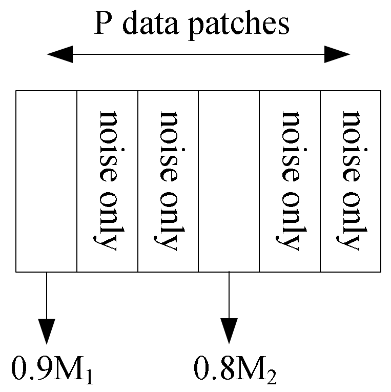
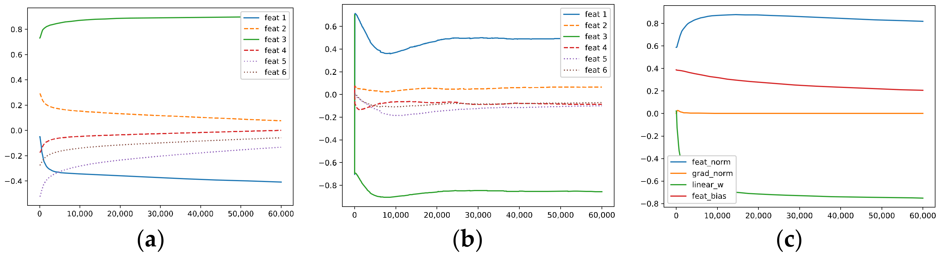
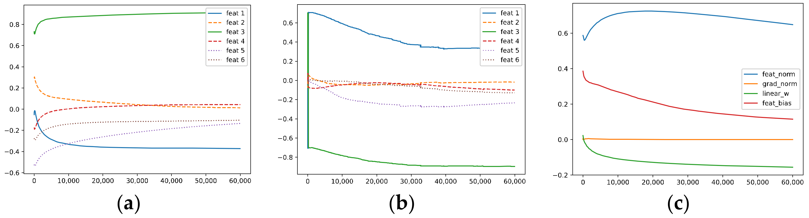
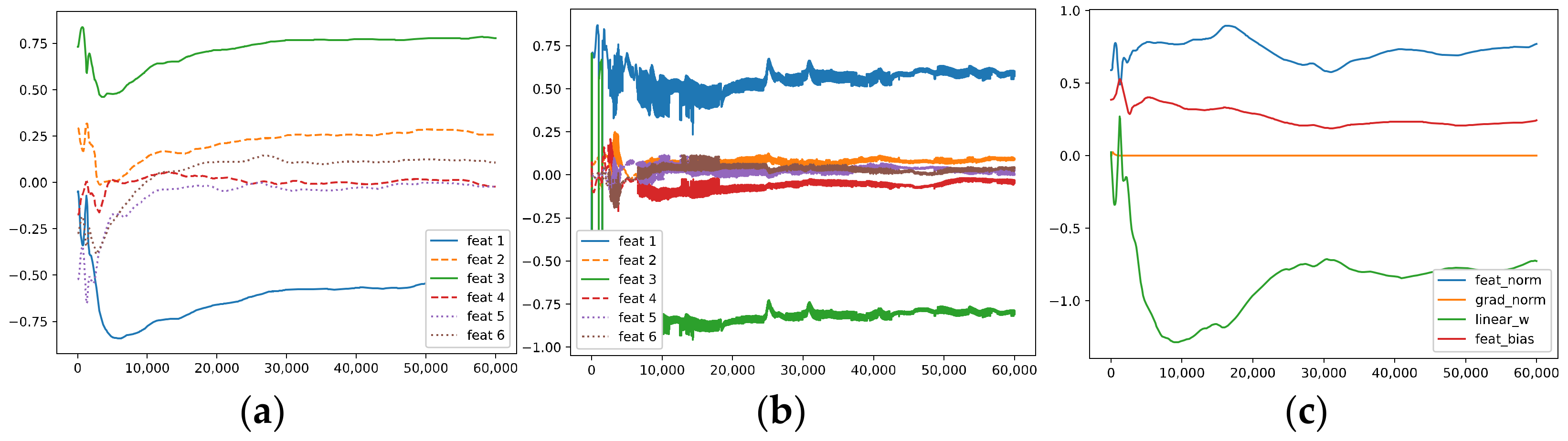
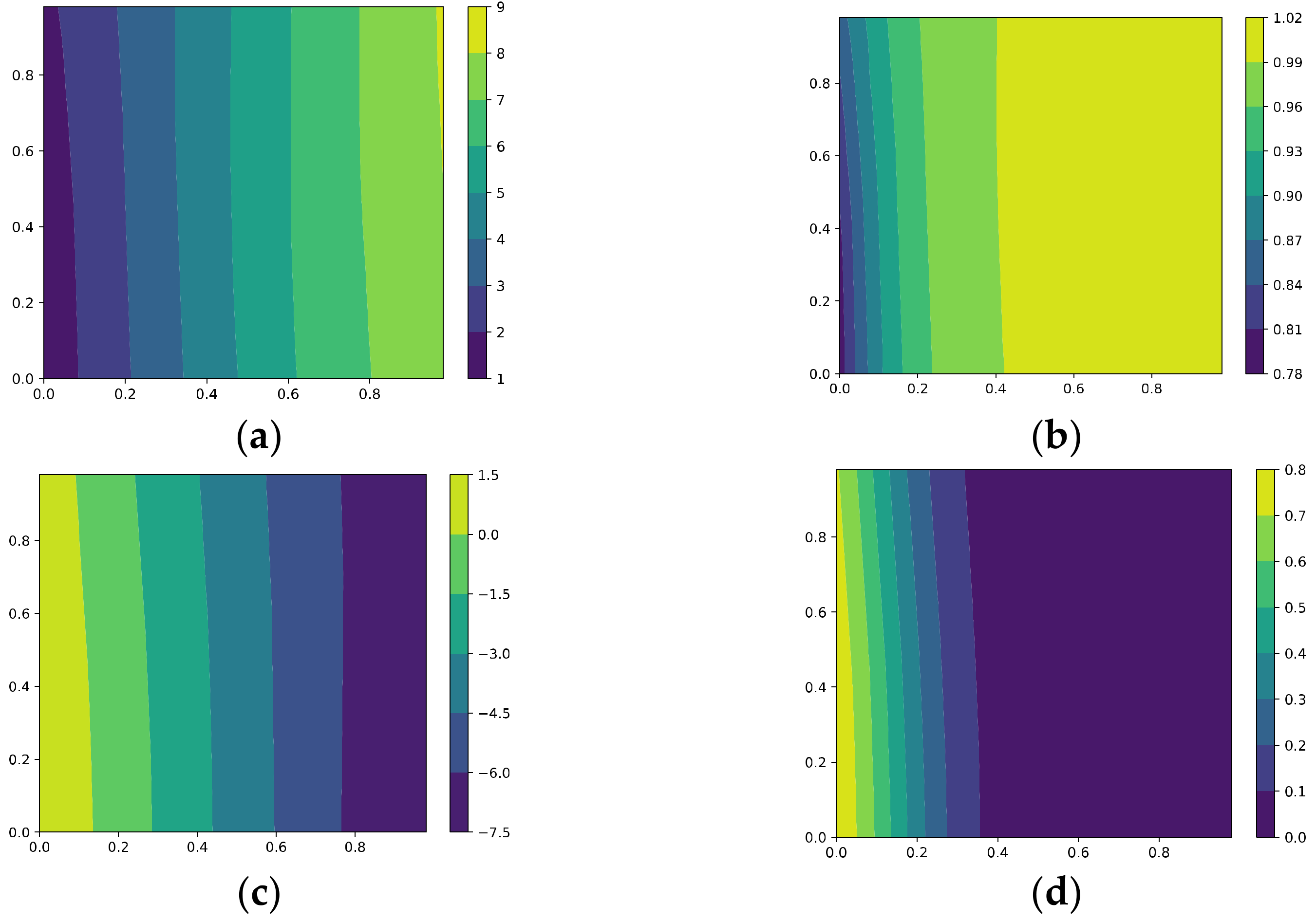
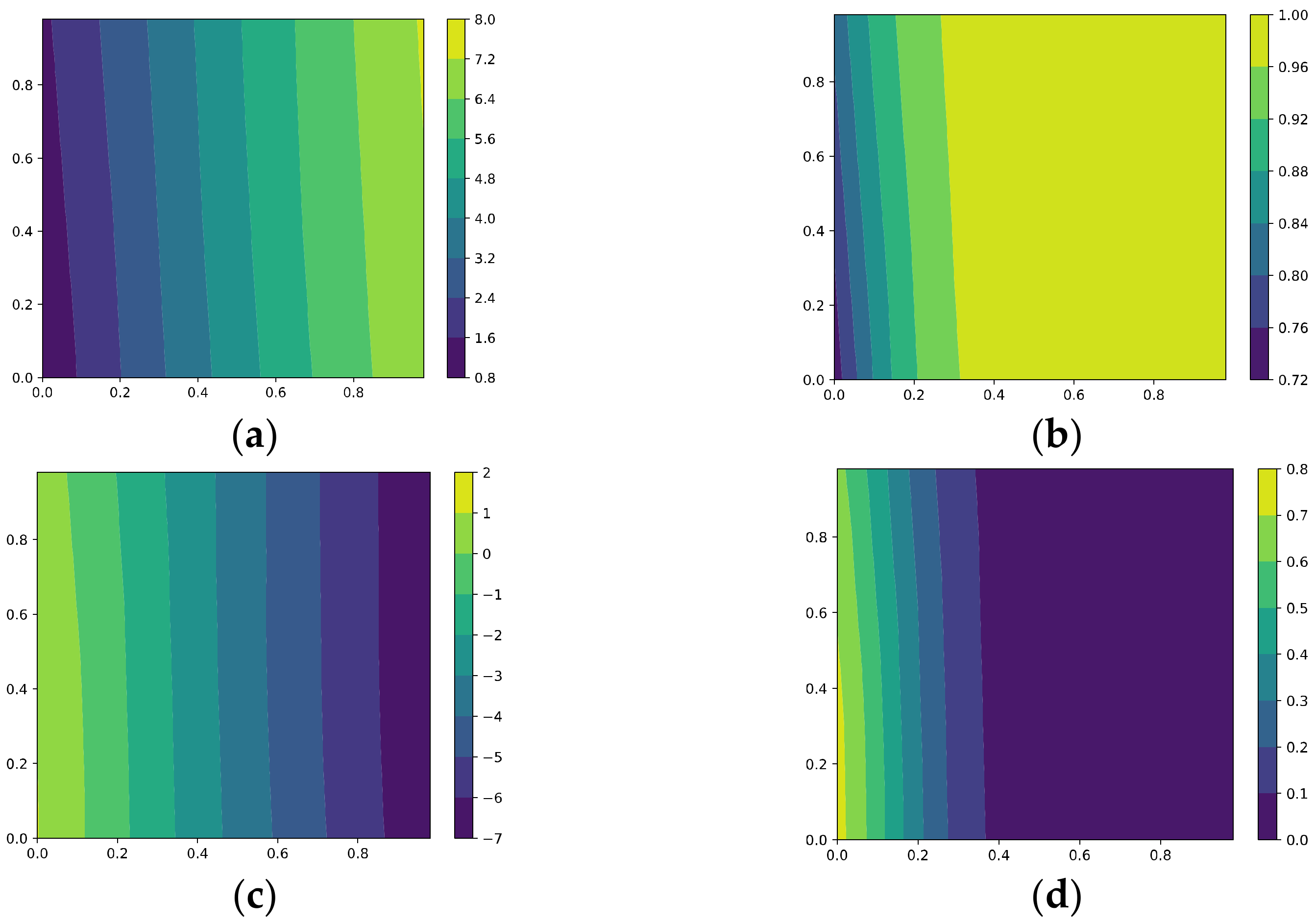
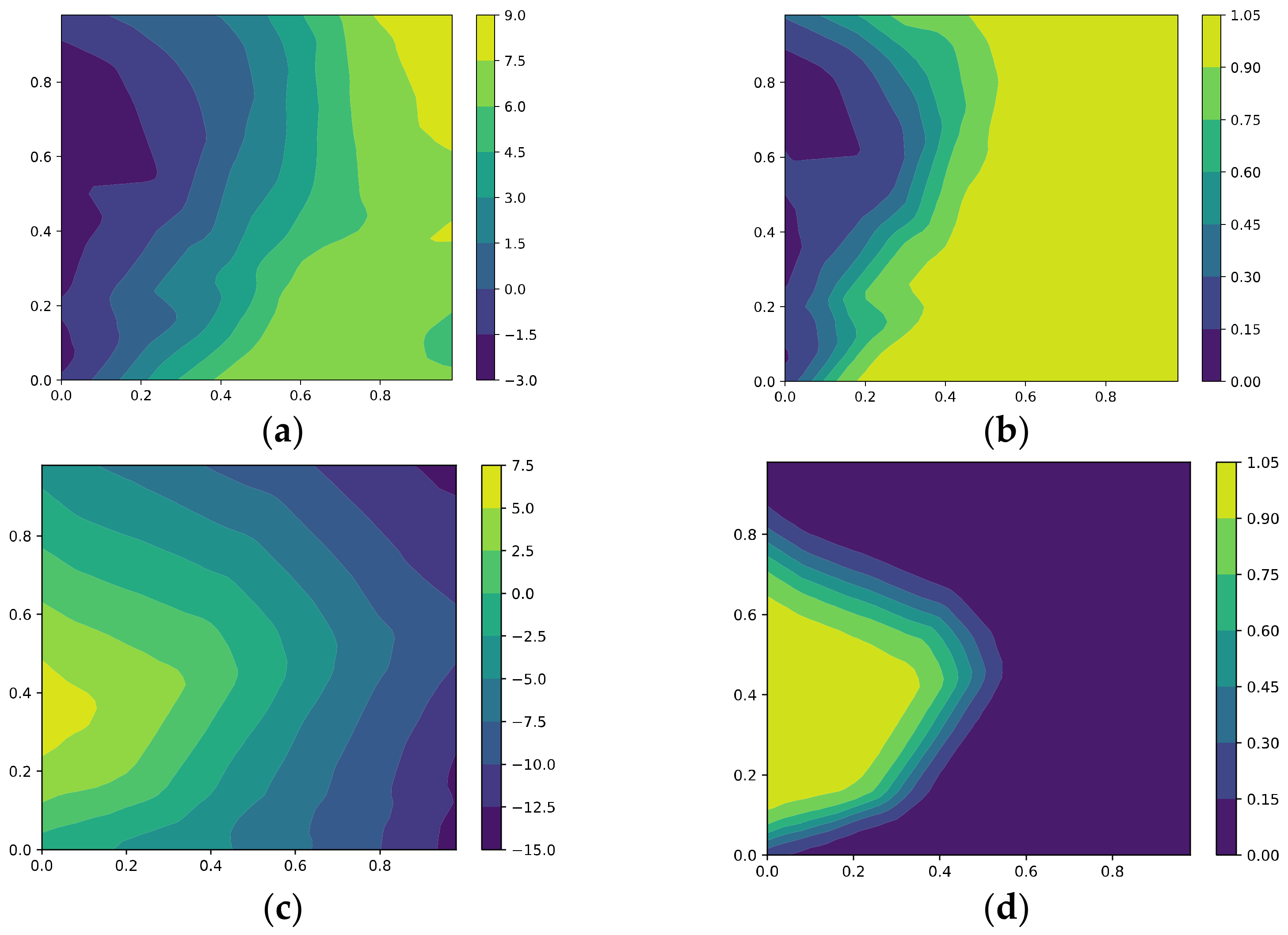
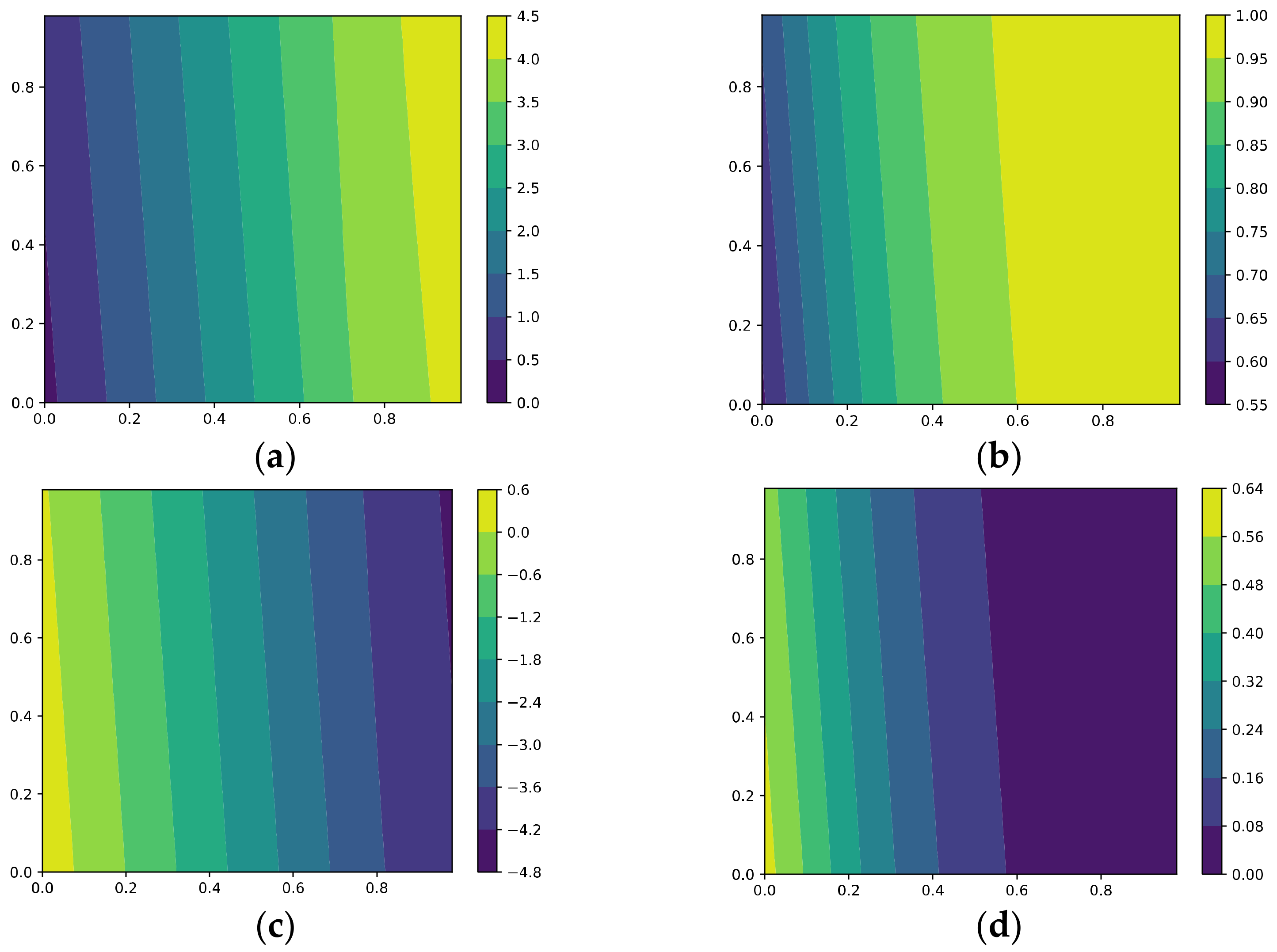
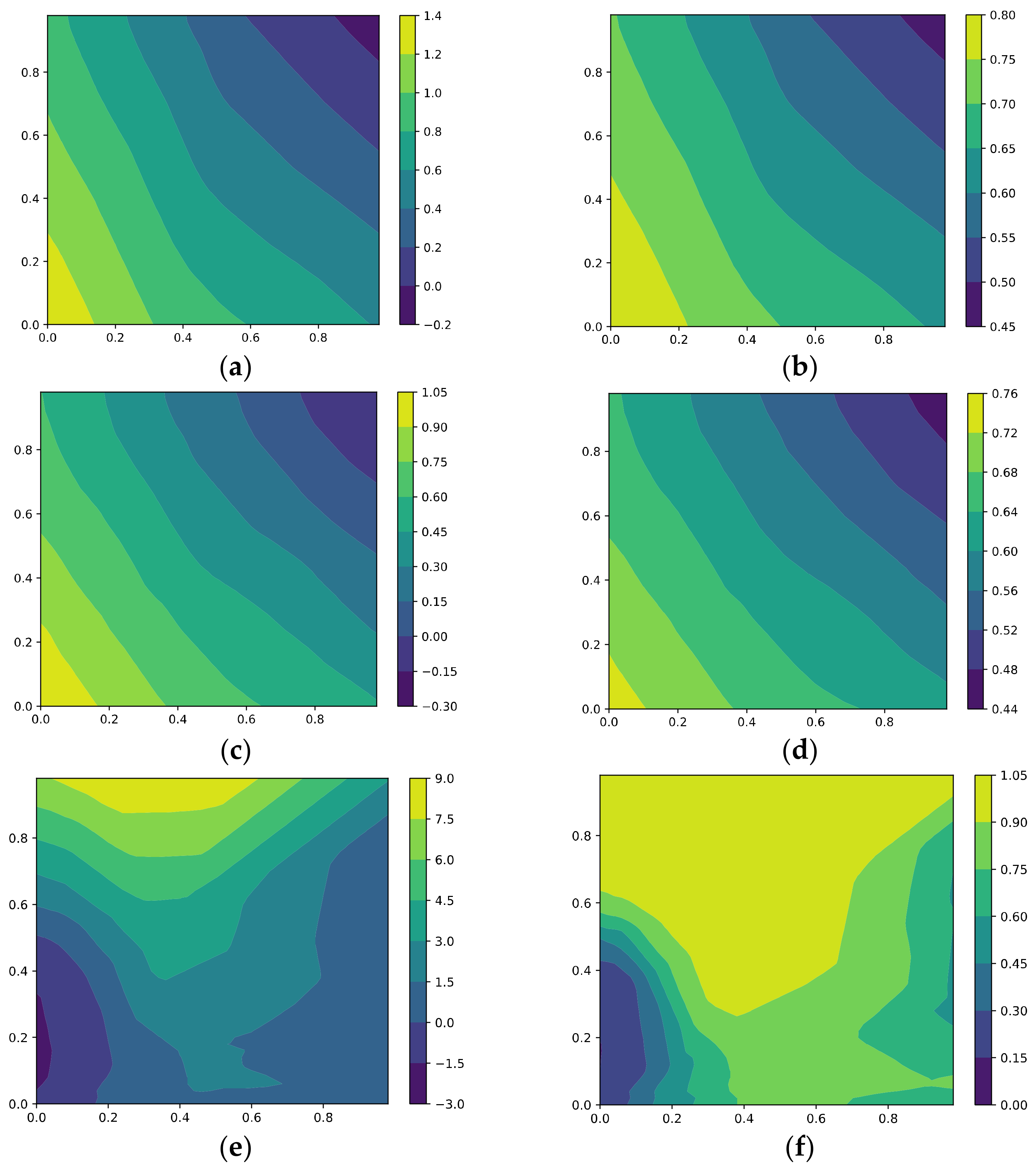
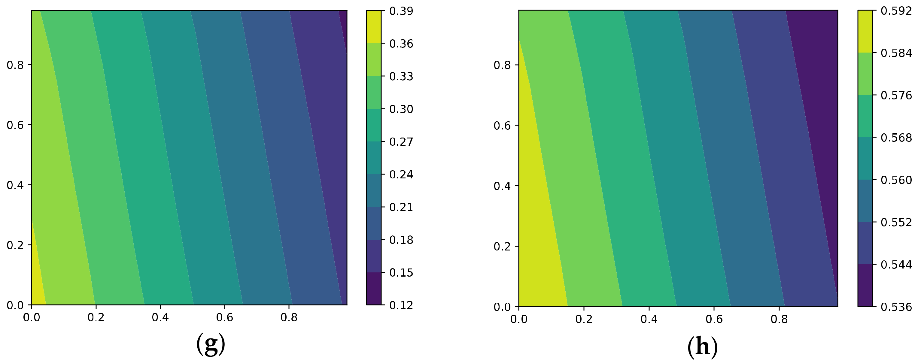
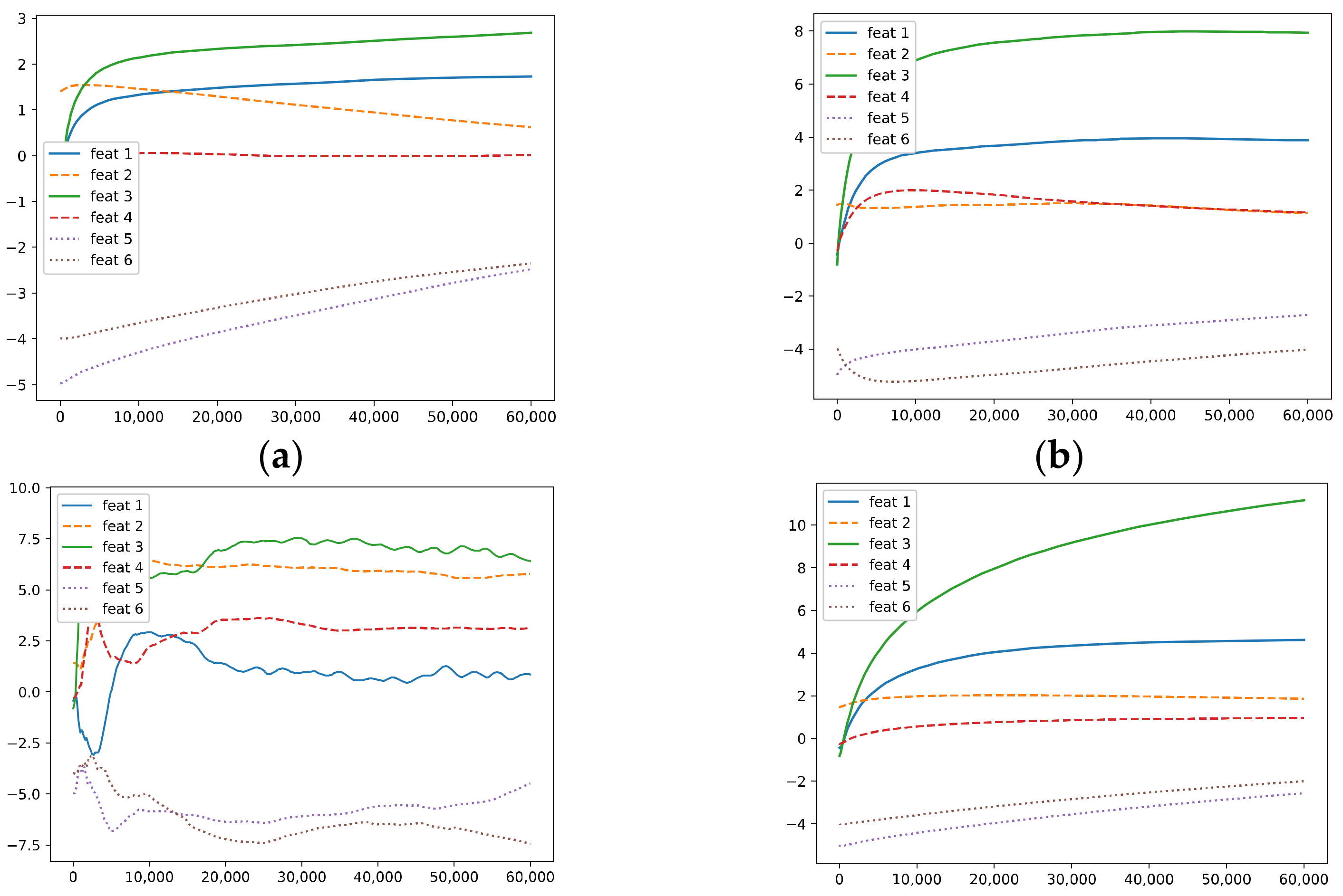
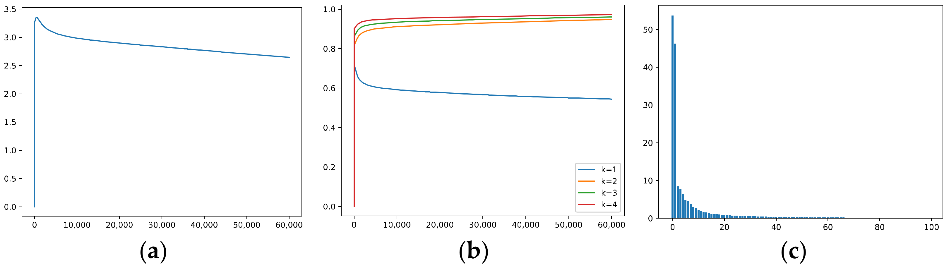
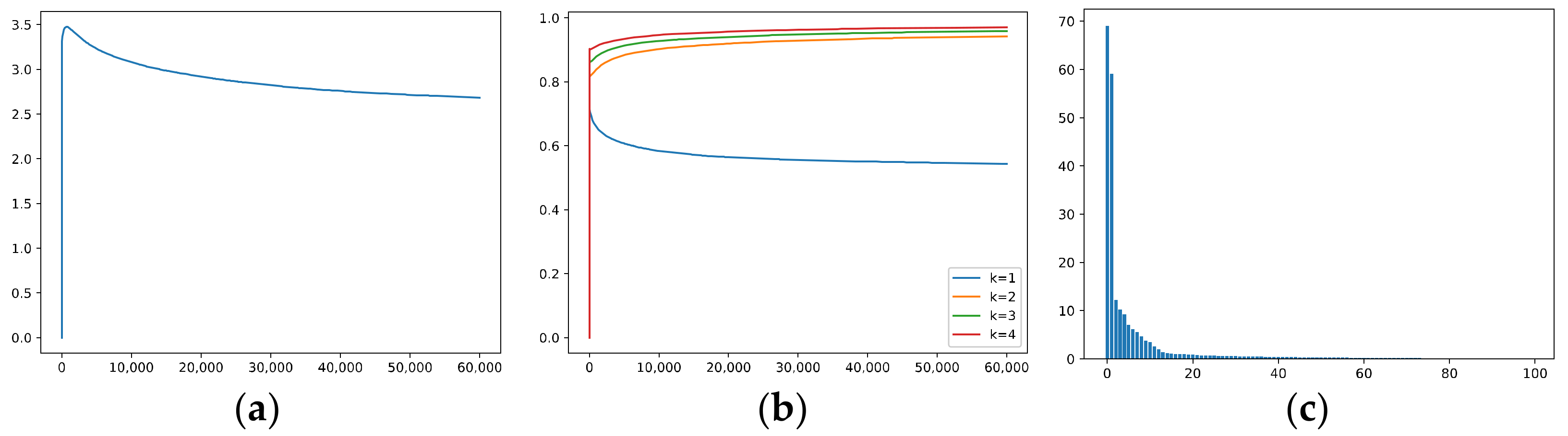
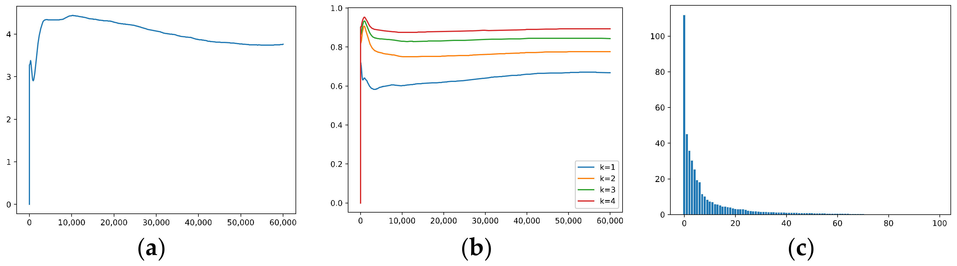
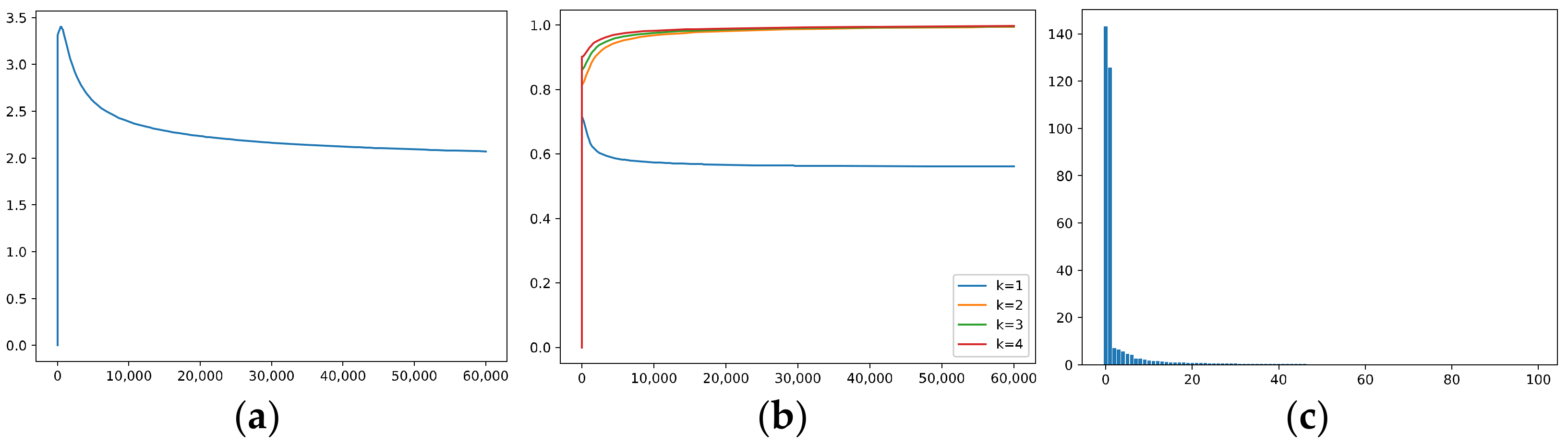
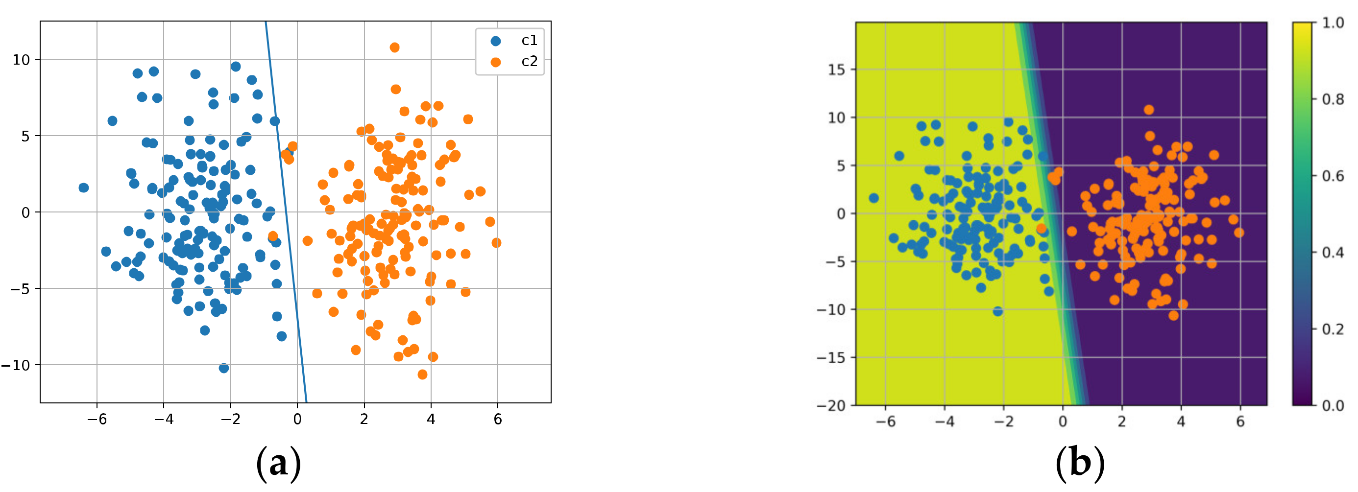
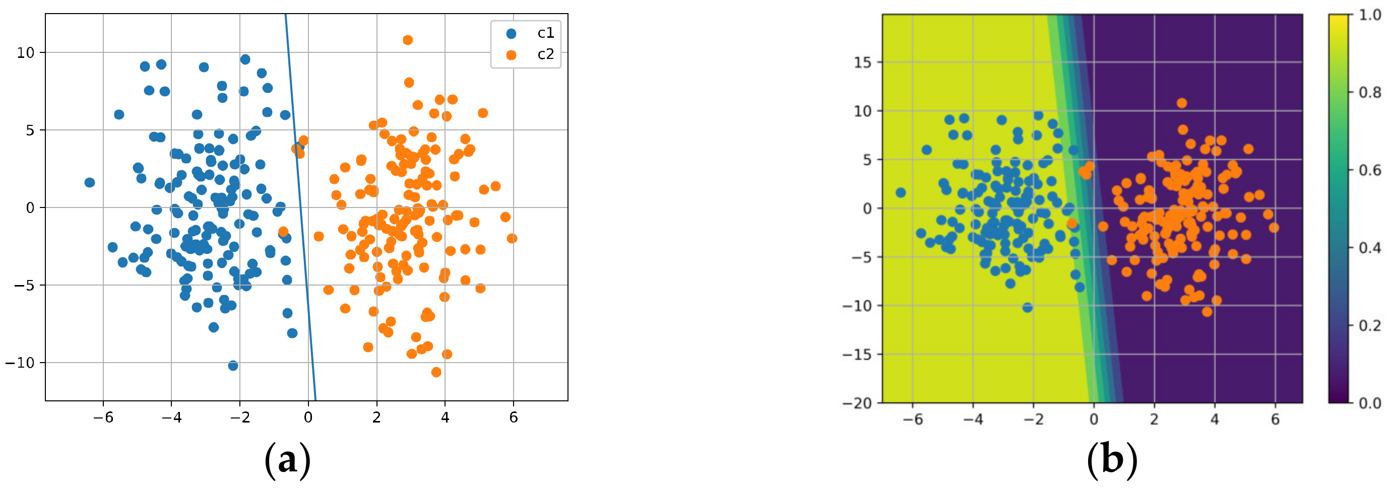
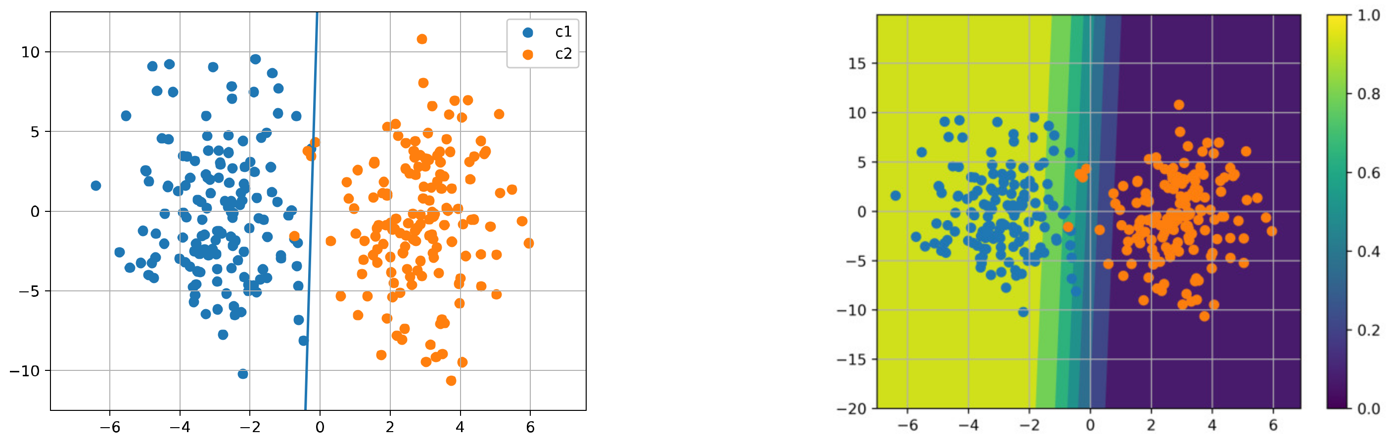
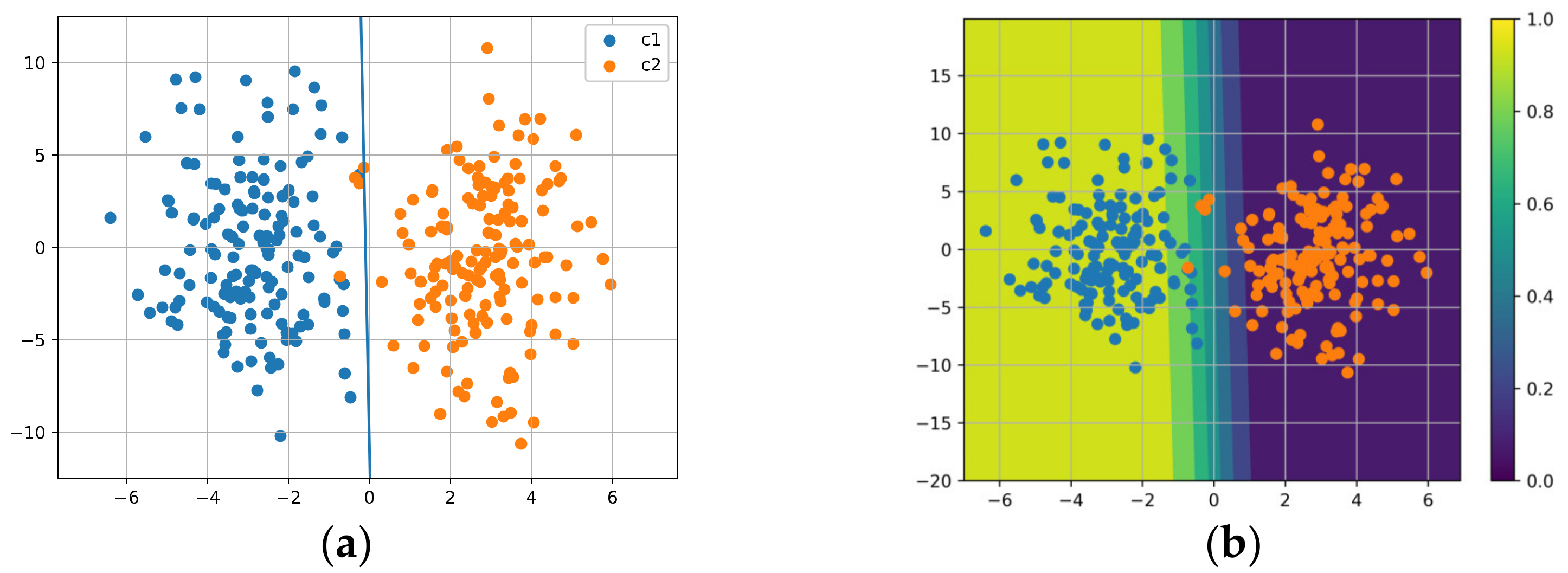
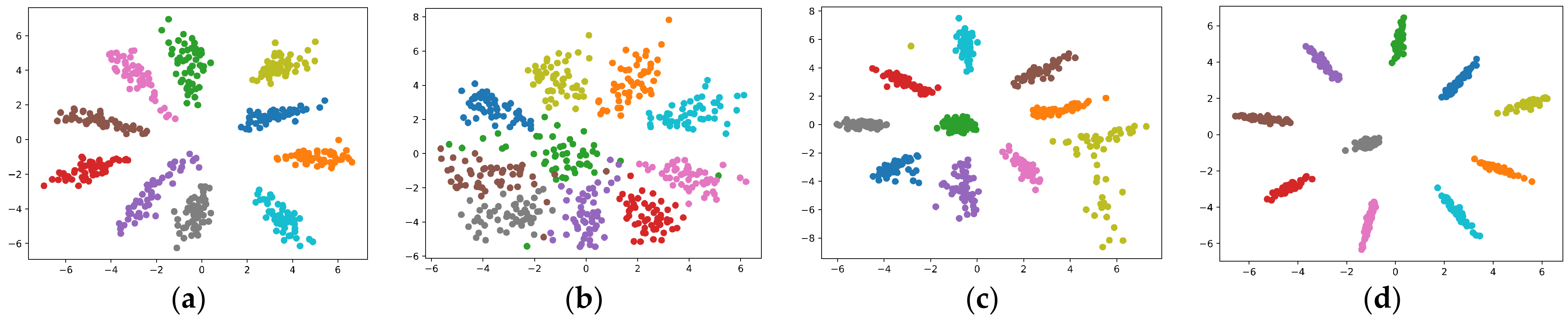
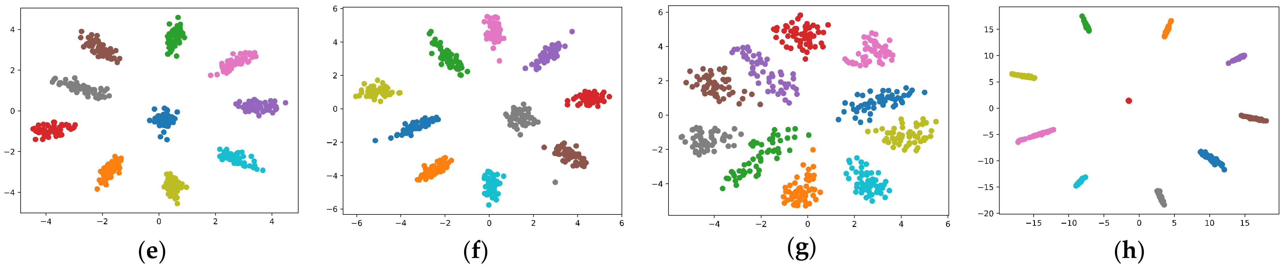
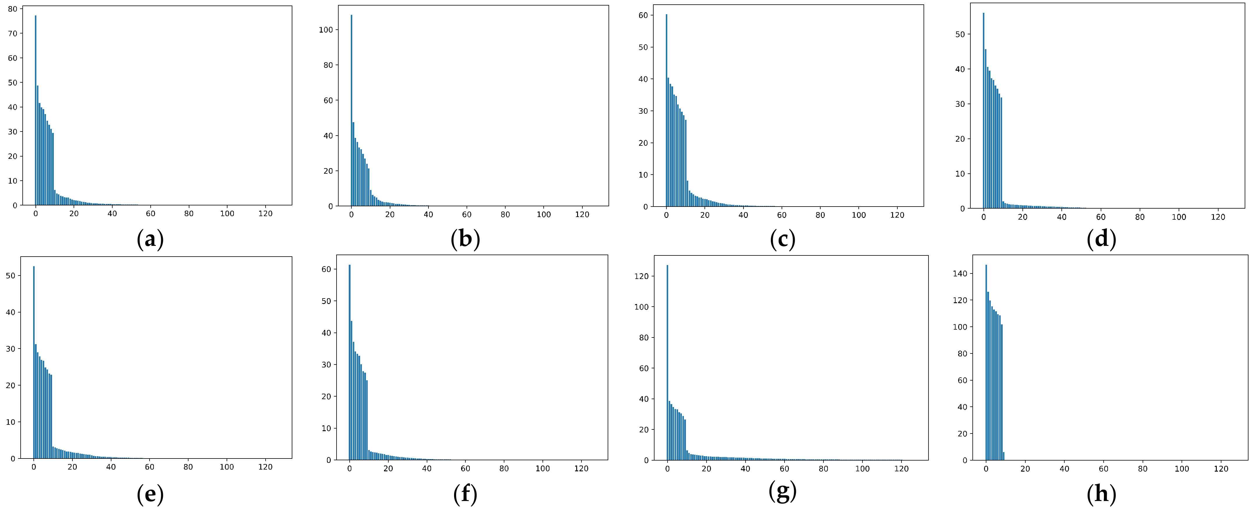
Table 1.
Comparison with previous regularizers. “Vanilla” includes batch normalization, dropout, and weight decay. The average test error and the standard deviation are reported. (We use the bold to highlight the smallest test error).
Table 1.
Comparison with previous regularizers. “Vanilla” includes batch normalization, dropout, and weight decay. The average test error and the standard deviation are reported. (We use the bold to highlight the smallest test error).
| Regularization | MNIST-250 | SVHN-250 | CIFAR10-500 | CIFAR10-1k |
|---|---|---|---|---|
| Vanilla | 7.1 ± 1.0 | 30.1 ± 2.9 | 39.4 ± 1.5 | 29.5 ± 0.8 |
| +Jac.-Reg [43] | 6.2 ± 0.8 | 33.1 ± 2.8 | 39.7 ± 2.0 | 29.8 ± 1.2 |
| +DeCov [44] | 6.5 ± 1.1 | 28.9 ± 2.2 | 38.2 ± 1.5 | 29.0 ± 0.6 |
| +VR [45] | 6.1 ± 0.5 | 28.2 ± 2.4 | 38.6 ± 1.4 | 29.3 ± 0.7 |
| +cw-CR [45] | 7.0 ± 0.6 | 28.8 ± 2.9 | 39.0 ± 1.9 | 29.1 ± 0.7 |
| +cw-VR [45] | 6.2 ± 0.8 | 28.4 ± 2.5 | 38.5 ± 1.6 | 29.0 ± 0.7 |
| +Sub-batches [15] | 7.1 ± 0.5 | 27.5 ± 2.6 | 38.3 ± 3.0 | 28.9 ± 0.4 |
| +Sub-batches + Top.-Reg [15] | 5.6 ± 0.7 | 22.5 ± 2.0 | 36.5 ± 1.2 | 28.5 ± 0.6 |
| +Sub-batches + Top.-Reg [15] | 5.9 ± 0.3 | 23.3 ± 1.1 | 36.8 ± 0.3 | 28.8 ± 0.3 |
| +FC_Reg (ours) | 5.3 ± 0.3 | 27.8 ± 1.3 | 36.2 ± 0.7 | 28.4 ± 0.3 |
Table 2.
Comparison of trace ratios.
| Regularization | Trace Ratios of the Representations |
|---|---|
| Vanilla | [0.3169, 0.4428, 0.5347, 0.6189, 0.7002, 0.7735, 0.8363, 0.8934, 0.9445, 0.9903] |
| +Jac.-Reg [43] | [0.5379, 0.6417, 0.7099, 0.7706, 0.8209, 0.8686, 0.9089, 0.9422, 0.9684, 0.9891] |
| +DeCov [44] | [0.2386, 0.3460, 0.4434, 0.5366, 0.6175, 0.6964, 0.7638, 0.8259, 0.8841, 0.9380] |
| +VR [45] | [0.3013, 0.4078, 0.4997, 0.5849, 0.6643, 0.7422, 0.8100, 0.8746, 0.9335, 0.9909] |
| +cw-CR [45] | [0.2001, 0.3326, 0.4374, 0.5364, 0.6252, 0.7113, 0.7902, 0.8650, 0.9338, 0.9983] |
| +cw-VR [45] | [0.3013, 0.4078, 0.4997, 0.5849, 0.6643, 0.7422, 0.8100, 0.8746, 0.9335, 0.9909] |
| +Top.-Reg [15] | [0.6253, 0.6835, 0.7317, 0.7781, 0.8220, 0.8608, 0.8971, 0.9313, 0.9637, 0.9883] |
| +FC_Reg (ours) | [0.1727, 0.3008, 0.4158, 0.5226, 0.6253, 0.7254, 0.8217, 0.9165, 0.9997, 1.0000] |
Disclaimer/Publisher’s Note: The statements, opinions and data contained in all publications are solely those of the individual author(s) and contributor(s) and not of MDPI and/or the editor(s). MDPI and/or the editor(s) disclaim responsibility for any injury to people or property resulting from any ideas, methods, instructions or products referred to in the content. |
© 2023 by the authors. Licensee MDPI, Basel, Switzerland. This article is an open access article distributed under the terms and conditions of the Creative Commons Attribution (CC BY) license (https://creativecommons.org/licenses/by/4.0/).
Share and Cite
MDPI and ACS Style
Chen, M.; Wang, D.; Feng, S.; Zhang, Y. Denoising in Representation Space via Data-Dependent Regularization for Better Representation. Mathematics 2023, 11, 2327. https://doi.org/10.3390/math11102327
AMA Style
Chen M, Wang D, Feng S, Zhang Y. Denoising in Representation Space via Data-Dependent Regularization for Better Representation. Mathematics. 2023; 11(10):2327. https://doi.org/10.3390/math11102327
Chicago/Turabian StyleChen, Muyi, Daling Wang, Shi Feng, and Yifei Zhang. 2023. "Denoising in Representation Space via Data-Dependent Regularization for Better Representation" Mathematics 11, no. 10: 2327. https://doi.org/10.3390/math11102327
Note that from the first issue of 2016, this journal uses article numbers instead of page numbers. See further details here.