1. Introduction
Any production system consists of different parts required to function well, to produce without losing performance. Over time, however, breakdowns might happen to any part of a system, which is unavoidable. These breakdowns might interrupt the production process and prevent meeting production goals, which might also lead to losing demand or profitability opportunities in the state where the product is demanded [
1]. Accordingly, the malfunctioning time of systems must be minimized. To minimize system breakdown time, spare parts must be accessible. On the other hand, buying and storing spare parts is often costly, and these parts are especially vulnerable to obsolescence risk [
2]. As a result, good spare part inventory management is critical in managing system costs. Furthermore, there are only a few suppliers of specialized spare parts. Indeed, if the main supplier does not provide spare parts or if supplies are disrupted, the part must be supplied by another supplier [
3]. This issue raises the price considerably and lengthens the delivery time.
Since single sourcing is rigid and supplier reliance is high, supply chain managers employ multiple sourcing to reduce costs and mitigate operational risks by using different supplier characteristics. Additionally, since it is hard to find the best replenishment approach for a multi-supplier model, practitioners and academics have long been interested in how to best execute and coordinate replenishment and inventory management with many varying supply alternatives [
4].
Multiple sourcing is a broad term that may relate to any inventory system or replenishment decision issue in which two or more supply sources, transportation modes, delivery alternatives, or transit speeds must be chosen [
5].
Many firms maintain many inventory items in practice, and scientific procedures and tools are required to efficiently handle such a large number of inventory items [
6]. As a result, researching the multi-product inventory management issue has real-world implications and is still a difficult topic to solve today. The multi-product inventory issue is now receiving a lot of attention [
7]. In most states, however, it is possible to purchase elsewhere, from an emergency supplier; for example, the desired part could be available in another company’s warehouse. Accordingly, it is vital to consider supplier disruption as a critical component of inventory management [
8]. As a result, one of the most important tools for dealing with supply disruptions is proper inventory management. For proposed and regular control of orders and inventories, obtaining values of two main parameters, including the amount of each order time and suitable date of order, is usually paramount [
9]. Different orders and inventory control systems must be designed in a structure consistent with each industry’s conditions to respond to the two factors mentioned above. It is evident that numerical values of the above parameters depend on several factors, including different inventory costs, consumption rate, certain or probabilistic (stochastic) consumption, and the required level of reliability to keep an inventory of any specific commodity [
10,
11]. They also depend on constraints acting on an industrial unit. Based on these factors and their impact on an industrial unit, different inventory control systems for various commodities at a time are defined.
As a result, order systems are classified into two categories: order point systems and periodic order systems. Several parameters, such as demand, demand locations, and the ability of centers to provide service and their usable capacity, were not accurately predictable due to the uncertain nature of some significant supply chain factors. As an outcome, effort is made to employ some techniques that take these uncertainties into consideration as much as possible while providing demanders with a high-quality response [
12]. Efficient and perfect supply chains are more subject to disruption, and efficiency and risk are inversely correlated. Organizations cannot merely focus on cost reduction for a long time, and supply chain investors must pay attention to how these capitals and changes affect the disruption in the supply chain [
13]. Besides, the studied disruptions are often general and do not take account of specific conditions and the reason behind the occurrence of disruption, while considering that these issues can significantly contribute to the selected strategy to reduce the effects and tackle the disruption [
14].
Nowadays, according to current competitive conditions, companies try to reduce their inventory level to reduce their costs. In inventory management and control of organizations, there must be a balance between spare part inventory level and cost and risk imposed by lack of spare parts when demanded. It is obvious that this spare part inventory level is affected by the device’s properties and reliability [
15].
Most previous studies have considered inventory maintenance with an assumption of unlimited access to spare parts [
10]. Considering that this assumption increases inventory costs, the costs can significantly be reduced by considering an optimal spare part inventory level [
16].
Polito and Watson [
17] developed a model that may be used to create a multi-echelon and multi-product distribution system. In a multi-product and multi-period inventory control, Moin and co-workers [
18] looked at the optimum ordering amount. Pal [
19] presented a stochastic inventory model with product recovery and inspection policy is incorporated for lot-sizing.
Murray et al. [
20] studied a price-setting and multi-product newsvendor with moderate assets capacity. Choi and Ruszczyski [
21] used a risk aversion hypothesis in their multi-product inventory model; however, their model also considered independent product requirements. Over the past few years, many researchers have prioritized the multi-product inventory model in their studies. Ramkumar and coworkers [
22] suggested a mixed-integer linear programming explanation to unravel this problem. Hosseinifard [
23] devised a linear penalty/bonus system to estimate optimal stocking resolution for choosing a strategic supplier by utilizing the stochastic dynamic programming technique.
Sokolinskiy [
24] suggested a stochastic optimization method for endogenous demand and inventory management regarding the inspection of the function of client defections and referrals. Mjirda [
25] presented a two-phase variable neighborhood technique for solving the problem, while Coelho [
26] proposed a branch-and-cut approach. Even though the prior models have assisted in the evolution of the operation theory for the multi-product inventory control issue, their optimum policy for the multivariate Markov demand perspective is still missing. Sethi and Cheng [
27] investigated the state-dependent policies of the inventory by using Markov-modulated lost and demand sales. Gharaei [
28] offered a mathematical model utilizing mixed-integer nonlinear programming for minimizing the total costs of both buyers and the vendor and optimal batch-sizing policy by taking into consideration the algorithm of augmented penalty. Khaniyev and Aliyev [
29] utilized their model in order to evaluate state-dependent policies with the asymptotic behavior of the ergodic distribution of the process. The optimum inventory model that has a limited capacity and rather observable Markov-modulated supply and demand procedures were investigated by Arifolu [
30] and Ozer and Atali [
31] using Markov-modulated production and demand quantity requirements to study a two-stage multi-item manufacturing system. Ahiska [
32] investigated the case of an uncertain source and managed to develop a stochastic inventory approach based on a Markov decision processes. Parker and Olsen [
33] devised a Markov equilibrium technique in inventory competition under dynamic circumstances while assuming that the equilibrium in a fixed infinite-horizon is a Markov perfect equilibrium. In addition, Barron [
34] studied a make-to-stock inventory/production system that was exposed to accidental conditions with moderate storage capacity and restrained backlog chances, while supposing that the entry of demand pursues Markov additive processes guided through continuous-time Markov chains. However, the theory of the Markov chain is utilized in all the aforementioned literature, all of which solely deals with a single item or multiple items with independent demand. Luo [
35] proposed a single-product mathematical model for controlling and predicting inventory systems, which includes a stable and unstable supplier. Asadi [
36] investigated a stochastic model to control inventory with respect to the Markov chain. According to the complexities of the proposed model, they employed two approaches, including a heuristic benchmark policy and a reinforcement learning method, to solve their model. Ye [
37] proposed an MINLP mathematical model for determining optimized inventory policy under disruption according to the Markov chain. They employed a two-stage algorithm to solve their complex model. Chin [
38] used the Markov chain in MINLP mathematical model for determining optimized long-term policy. Patriarca [
39] presented a Multi-Echelon Technique for inventory of Recoverable Item Control (METRIC) to investigate the potential use of a Weibull distribution for modelling items’ demand in case of failure. Milewski [
40] focused on the economic efficiency of decentralized and centralized inventory strategies of distribution products in terms of both internal efficiency of firms and external costs of logistics processes.
In line with the studies conducted over the past years in this field, research gaps in the studies carried out by researchers remain. Most of the research focused on one supplier and one product, while in real world cases, there are more suppliers considering their situations (reliable–unreliable) that provide a variety of products [
36]. It is critical to include exploring the interdependencies between up/down probabilities for the unreliable supplier across periods. Moreover, investigating the performance of different optimization methods to find more suitable methods to solve inventory models is vital [
38]. Uncertainty in demand and other parameters, which has an undeniable effect on the models, is not widely considered [
35].
Therefore, this study aims to propose a multi-product mathematical model to determine optimal inventory policy by considering the Markov chain. Moreover, two reliable and unreliable suppliers with disruption probability in the supply chain were also taken into account. The demand for all products will also be uncertain. Given that the proposed model will be highly complex, several meta-heuristic methods will be proposed to solve the problem. In order to assess the model better, a state study is also implemented, and the best assessed meta-heuristic method is employed to solve it. More specifically, in this research, Grey Wolf Optimizer (GWO), Genetic Algorithm (GA), Moth–Flame Optimization (MFO) Algorithm, and Differential Evolution (DE) Algorithm are applied to solve the model faster and more accurately. To evaluate their efficiency, two factors including numbers of iterations and spent time are investigated to discover which solution method is more useful to solve the inventory models.
Table 1 shows this research’s contributions in comparison to the most recently published articles which are completely relevant to this paper. Regarding all these gaps reviewed, the present research aims to cover these neglected concepts in mathematical inventory models. In what follows, some important innovations of the research are stated:
Design of a mathematical model for determining optimized multi-product policy with the Markov approach, designing a novel mathematical model to optimize multi-product inventory control considering the Markov system under disruption and uncertainty;
Considering lead time as an objective function;
Considering two reliable and unreliable suppliers with different costs and delivery times;
Using four meta-heuristic methods to estimate their performance to solve a real case inventory model;
Considering uncertainty in demand;
Proposing a state study in the production of automobile spare parts.
2. Materials and Methods
One retailer and two kinds of suppliers are assumed in this research; one is reliable, and the other one is unreliable, providing the demanded item at a lower price compared with the reliable supplier. The following method specifies an unreliable supplier’s accessibility process. The status for an unreliable supplier can be “appropriate”, which means they can take orders, or the status can be “inappropriate”, which means they are not taking orders. Based on the inventory, the retailer demands the preferred price from a single supplier or both of them. The unreliable supplier’s status and circumstances are dependent on the demands at the start of each time period. An order that was made at the start of a time period will be shipped at the end of that time period. A certain delivery and specified value at the end of the time period are guaranteed for the reliable supplier. An unreliable supplier cannot take orders from the retailer if it is not currently at an appropriate status. An unreliable supplier’s status is specified after the demand. If the appropriate status changes to inappropriate at the final days of the time period, the order will be canceled, otherwise, the unreliable supplier will deliver the order. In the case of an order to an unreliable supplier, the fixed ordering fee (internal running cost of constructing an order) is reimbursed at the time of the delivery.
Demand during a period is independently and equally divided between distributers. Demand and system cost parameters are constant and do not change over time. Any unit in the inventory during a period has a maintenance cost. If the inventory is available, each required unit on the unit will be subtracted from the inventory. Otherwise, the demand is reordered and restored. Any demand higher than this limit is missed, and the missed selling cost is imposed on the retailer. The constraint that acts as the lowest limit in the inventory limits this problem to a Markov chain process model, which can be solved by overloading computation.
The activities that are carried out in a period are listed as follows:
The system status depends on inventory at the beginning of the period;
Making a decision regarding the amount of order;
Demand is dispatched during the period and happens from the beginning of the inventory time period;
The order dispatched to an unreliable supplier is received at the end of the period;
The status of unreliable suppliers is determined at the end of the period;
The cost of missed order demand is calculated.
2.1. Mathematical Modelingl
The presented mathematical model in this research aims to determine order strategy, such that the total expected cost for any period is minimized, which includes the following states:
Order cost is fixed and is paid to each one of the suppliers for each dispatched order;
The number of order units (number of buying); in the research problem, it is assumed that the number of made orders is a linear function;
Maintenance cost; the cost of each unit for the unreliable supplier is less than the reliable supplier;
The cost of missed sales is considered in the number of missed sales as a linear function;
Shortage is not allowed;
Products are not independent of each other;
Preparation time is considered a uniform distribution function.
2.1.1. System Status
According to the mentioned states, the system status is displayed as , where indicates inventory level and is supplier status. has values equal to one or zero, which indicate appropriate or inappropriate supplier status, respectively. The inventory level of retailers is between , and indicates the capacity of the retailer’s storehouse.
2.1.2. Decision Variables
Supposing that
vector equals the order amount to two studied suppliers, and
is the status of the system, the value of the order to two suppliers is indicated as
As, whose value is determined according to the retailer’s storage capacity and the status of the unreliable supplier, which is expressed as the following equation:
2.1.3. Transition Modes and Transition Probabilities
Two fundamental Markov chain processes describe the transition status. One is related to unreliable suppliers and the other is related to inventory status. The first is independent of the second.
| : | The number of orders to the unreliable supplier |
| : | The number of orders to the reliable supplier |
The status of an inappropriate supplier is controlled by a two-status Markov chain process with transition probability matrix,
, where
indicates the probability of a transition status of an unreliable supplier from
to
during a period. In particular, we define
as the probability of an unreliable supplier from up to down (from an appropriate status to an inappropriate status in demand-supply), from one period to the next, and
is the probability of inappropriate status from down to up, from one period to the next.
Demand at each period for each product equals
, whose occurrence probability is indicated by
probability function. According to the system status, which is
at the beginning of the period, the demand value is defined according to
, which equals
for each product. It is expressed as the following Equation when the system status changes to
demand for different products according to unreliable supplier status.
| : | Status of the inappropriate supplier is appropriate. |
In Equation (2), if the supplier remains unreliable during the period, it equals 0. Otherwise, it equals 1.
It is worth mentioning that when the status of the unreliable supplier changes from appropriate to inappropriate, the value of the order to the unreliable supplier is canceled (
).
In Equation (4), if the status of the unreliable supplier changes from appropriate to inappropriate during the period, it equals 0. Otherwise, it equals 1.
2.1.4. Markov Process, Markov Chain, and Markov Property
The Markov property, often known as the non-aftereffect property, specifies that the process state is known at a certain time
t. At the point
t1 >
t, the state at time
t1 is unrelated to the conditional probability distribution and is only concerned with the condition at time
t [
41].
The conditional probability distribution (CPD) function, which can be represented as follows, is used to explain the Markov property [
42]:
The random process
has a state-space of
. If, at any point
n in time
t, that is
, and under the
condition, then the CPD function of
equals the conditional distribution function
under the
condition:
The process
is known as a Markov process because it possesses the Markov property. A Markov chain is a Markov process with discrete state and discrete time in general. The following is how mathematical terminology describes it [
43].
The random process
has a state-space of
. It meets the following criteria for all
m non-negative integers
any natural number
k and any
:
The stochastic process is known as the Markov chain.
2.1.5. Transition Probability
The random process
has a state-space of
. Additionally, the probability of an n-step transition of the time m is defined as the likelihood that the model is moved to the state j via n steps when the system is in the state
I at time m, as indicated below:
When , may be denoted as , and the transition probability of the Markov chain is called .
The transition probability
satisfies the two features listed below:
The literature theorem proves that the Chapman Kolmogorov formula is satisfied by the n-step Markov chain transition probability, i.e., for each positive integer
h,
l:
A recursive technique may be used to generate the following equation:
A single-step transition matrix may be used to immediately create a matrix of Markov transition from Equation (7), offering a straightforward way of calculating the transition probability.
2.1.6. The Markov Chain’s Ergodic Property
If there is a transition probability limit of the Markov chain which is unrelated to i, then the ergodic property of the Markov chain is
Furthermore, it can be shown that for each
, there is
, i.e., the Markov chain is ergodic. Moreover, the limit distribution
is the only solution to the equations
under the conditions of
[
42].
2.2. Solution Methods
In this section, four solution methods are presented and described briefly which are applied for solving the mathematical model. The solution methods include Genetic Algorithm (GA), Differential Evolution (DE) Algorithm, Grey Wolf Optimizer (GWO) and Moth–Flame Optimization (MFO) Algorithm.
2.2.1. GA Solution Method
Genetic algorithm is a natural-principles-based heuristic evolutionary solution approach that may be used to solve hybrid search and optimization problems. There are two types of GA: continuous and binary GA. The algorithm’s whole set of rules may be found in [
40].
2.2.2. DE Solution Method
Mutation, initialization, recombination, selection, and crossover are the five major processes in this method [
41]. The starting parameter is haphazardly set in specific regions, containing lower bounds and upper bounds, to be optimized by the variables in the initialization process. Furthermore, both the recombination and mutation processes are aimed at producing a number of population vector trails. Additionally, the crossover aims to arrange a parameter value crossover vector that is replicated on two vectors, the mutation vector and the original vector. The next step, the selection process, is used to separate the vectors so that they may be utilized as the population for further iterations [
44].
2.2.3. GWO Solution Method
The Grey Wolf method is based on the grey wolf’s natural leadership hierarchy and hunting process. To imitate the leadership system, four sorts of grey wolves are used: delta, omega, beta, and alpha. Furthermore, the key processes of hunting are supposed to be seeking prey, surrounding the prey, and assaulting the prey in this algorithm. Mirjalili [
34] goes into detail about this method. As a consequence, while configuring the algorithm, the agent’s number is assumed to be 6, and the findings are verified using the benchmark test performer, which is specified in [
45].
2.2.4. MFO Solution Method
The Moth Flame method is a night-time moth fly behavior-inspired optimization approach. Mirjalili [
45] explains how this optimizer was inspired by transverse orientation. The benchmark test function, which is specified as F8 [
35], is used to verify the findings, and the dimensions’ number in this optimization is regarded to be six for this approach.
3. Results
The input values to the model are collected based on the case study of the South Pars Complex Company. The model we are discussing is a two-level supply chain under a vendor inventory management strategy. A number of retailers, each of which has a definite demand, at regular intervals, order a fixed amount of a type of product to the seller. In other words, the demand of retailers is discrete and the period that this demand is met at the beginning of each period. For direct delivery of these orders from the seller to the retailers, there are different schedules. The seller also orders a fixed amount to the main supplier at specified intervals to meet the retailers’ demand. In
Table 2, the input values of the parameters of each product are presented separately. In order to model the uncertainty in procurement time for eight products, procurement time is considered as the probability function in
Table 3.
For solving the presented mathematical model, a Dell laptop with 8Gig RAM, Intel Core i7 CPU and Microsoft Win10 is used. Moreover, coding and model solving by metaheuristic methods are performed in MATLAB software. Moreover, to achieve the exact and optimum solution, small size and medium size problems are solved by GAMS software and CPLEX solver. Before solving the real case study, which is a complex model, to validate the solving methods, the model is solved based on some small and medium size problems. To do so, the model is solved with small and medium problems by four mentioned meta-heuristic solution methods and the exact solution of CPLEX to compare their performance by the exact method. As shown in
Table 4, all of metaheuristic methods run the problems with marginal variation. However, regarding the
Figure 1, the GWO method was able to find the best answer with minimum variation.
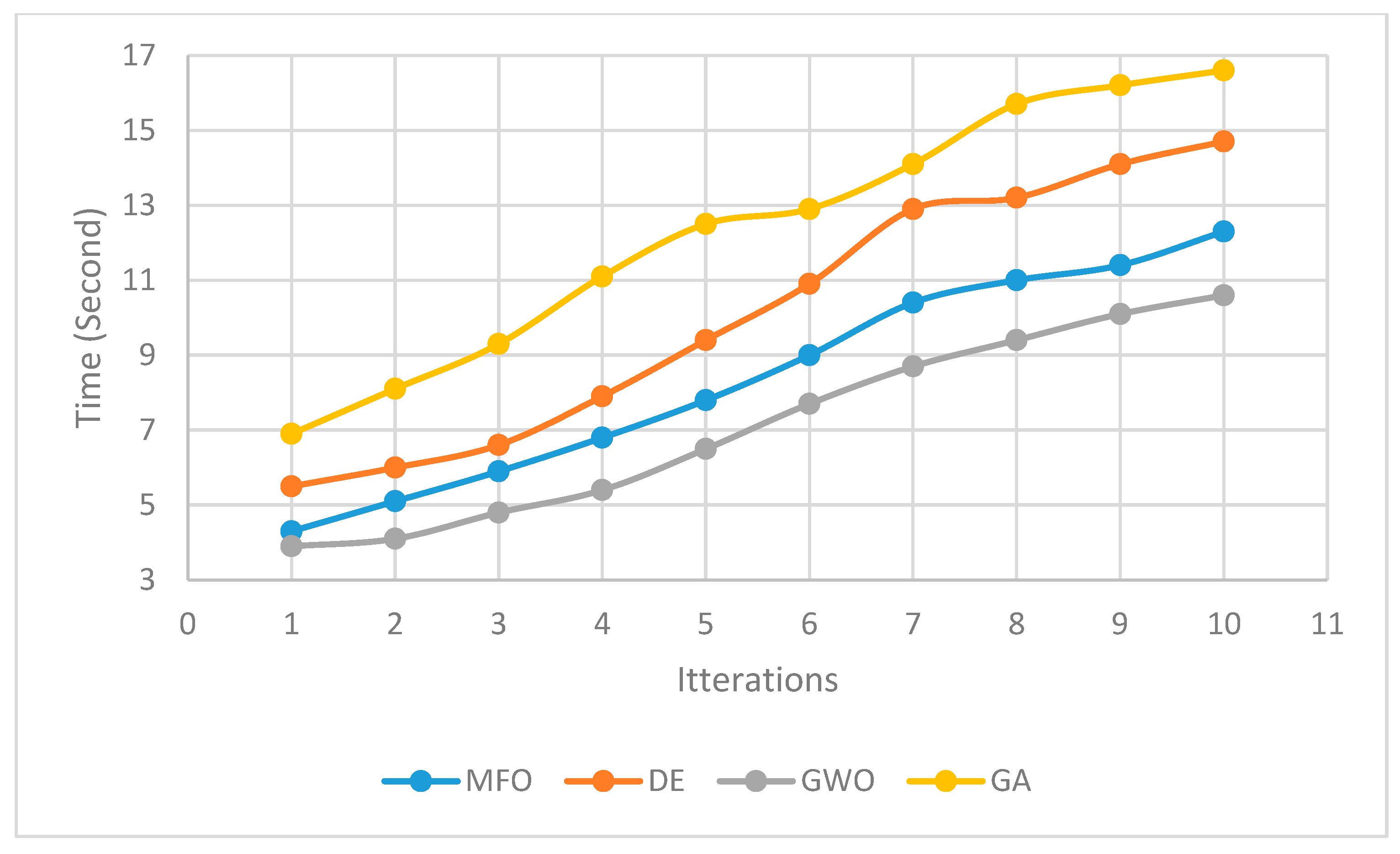
After performance evaluation of the meta-heuristics methods, they are applied to solve the real case model to optimize a complex problem. Output data which are generated by the mentioned solution methods are investigated.
As can be seen in
Figure 2 and
Figure 3, the GWO algorithm demonstrates a more proper answer compared to the other optimization methods. The preparation time and the financial costs have been considered in the optimization, where the optimization of each is not sufficient, and both factors should be taken into consideration together. The MFO, GWO and DE algorithms obtained the best cost function, but there is a difference in the lower convergence time of the GWO algorithm. The maximum passed the time for the executed algorithms is relevant to the GA with the maximum spent time.
As can be seen from
Figure 1, the convergence of the objective function for different solution methods is such that in the sixth iteration none of them were able to converge continuously. In the sixth iteration, the GWO algorithm was able to reach an acceptable level of convergence, and in the seventh iteration, it was also able to maintain this convergence. The MFO algorithm, which had the worst result of all the algorithms in the first iteration, converged very quickly in the next iterations, and finally in the eighth iteration, it converged faster than the other two algorithms. On the other hand, the two MFO and GWO algorithms, which performed better in convergence, recorded almost the same time in the first iteration. It was GWO that recorded the shortest convergence time. The GWO algorithm not only performed better in convergence, but was also able to do so in less time.
Before providing the optimal value for each introduced product, defining some explanations regarding the different transition states is required. As discussed in the model of the research problem in
Section 2, there are two states for ordering the products.
First state: When the unreliable supplier state is improper, all demands are supplied by the reliable supplier in entire states. With respect to the policy, we have the following: The orders level is equal to the maximum inventory level of the products that the reliable supplier can supply; if the demand exceeds the supply capacity, the demands are retarded.
Second state: When the unreliable supplier is in the proper situation, the four following states will occur:
- ○
State 1: With respect to the lower supply cost of the unreliable supplier, the demands are supplied merely from one supplier. With respect to the ordering policy, the maximum order level could be supplied.
- ○
State 2: The demand should be satisfied from both suppliers. In this state, if the demand is lower than the capacity of the reliable supplier, the remaining demands from the unreliable supplier are satisfied to the level.
- ○
State 3: The required demands are supplied from the two suppliers. In this state, before the demand, each supplier’s inventory is investigated. Then, concerning the available inventory level, the two suppliers supply the required demand.
- ○
State 4: The demand is supplied merely from the reliable supplier.
Given that the reliable supplier in the state four supplies all spare part demands, the demand is missed in several states, which imposes a cost on the system. This increase in the cost indicates its effect on the whole system, as shown in
Table 11.
In the third state, given that inventory of both suppliers is examined before making an order, the missed sale cost is zero. The total system cost is insignificant in this state compared to the fourth state. The only advantage of this state is the lack of missed sales.
Since a reliable supplier first supplies the demands, maintenance cost is reduced in the second state. Accordingly, as indicated in
Table 11, the system cost is reduced significantly compared to the third and fourth states.
In this state, given that unreliable suppliers supply all demands, the probability of missed sales is increased. However, due to the low cost of buying from this supplier, the total cost of this state is significantly lower than the previous state.
According to both the defined states at the beginning of the problem and the optimal values based on the ordering policies indicated in
Table 5,
Table 6,
Table 7,
Table 8,
Table 9,
Table 10,
Table 11 and
Table 12, the optimal value for all of these products is indicated according to four states in
Table 11. According to
Table 13, it is evident that the fourth state imposes the maximum cost on the system since, as mentioned earlier, the orders are supplied by reliable suppliers in this state. Accordingly, due to the difference in costs between two suppliers (the cost of buying a product from a reliable supplier is greater than buying a product from an unreliable supplier), this cost is greater than other states.
Based on the final reports, when it comes to reliable supplier disruption under uncertain conditions, there is no choice but to order from the unreliable supplier to meet demands. It is obvious that the cost of unreliable resources is higher that reliable one and the delivery time is less reliable. However, the company will consider these flaws and use the unreliable supplier to meet the demands of critical spare parts, since the waiting time for a comeback of the reliable supplier is not neglectable and the time lost due to the disruption causes the loss of demand.
4. Conclusions and Future Work
Planning and control of inventories are essential activities in supply chains and logistic systems. Hence, various studies and research have been conducted in this field. In terms of supply and demand, the issues in inventory planning are divided into two categories. The first category is inventory control, along with determining price. In conventional methods, determining price is the responsibility of the operational section, and pricing policies are separately determined by the marketing section. However, in order to maximize total profit, the policies and pricing must simultaneously be taken into account. Indeed, determining a suitable price is a complicated process, and organizations must have knowledge of operational costs, current customers, and future demand to be able to adjust and balance prices with minimum costs.
The second category is multi-objective models. Most of the inventory models cover the concept of different costs and services in one objective, and conventional methods are employed to solve them. On the other hand, one of the known features of trade in today’s world is a variety of decision-maker wishes. In multi-objective problems, the decision-maker aims to simultaneously maximize or minimize two or several objectives. This type of model has been employed in various fields, while few multi-objective problems have addressed inventory control.
In this study, the inventory model is designed under the disruption condition of suppliers for supplying critical spare parts based on the Markov chain process model. Logistic time, time horizon, and shortage are considered probable, limitless, unallowed, and completely restored. Demand is considered as a function of price. The proposed model is complex. Accordingly, the optimal system cost, ordering policies, and reorder point must be determined. Moreover, a real state study and sensitivity analysis were carried out on the main parameters of the model. Since most of the previous research applied simple optimization methods, this paper decided to implement four different meta-heuristic algorithms to solve the mathematical mode. Based on the output, all four methods work well, though the GWO method was the best method to solve the inventory policy decision making model. Moreover, contrary to the articles that emphasized the use of reliable suppliers, outputs of this research show that under uncertain conditions and disruption of reliable suppliers, it is not possible to meet all demands just by relying on reliable suppliers, because the waiting time for a comeback of the reliable supplier is not neglectable and the time lost due to the disruption causes the loss of demand. Regarding the optimal value of variables in presented tables, it is clear that companies should consider the unreliable supplier when the reliable one is under disruption, even if this approach costs more.
This article attempted to cover neglected aspects to improve previous research; however, there were some barriers in addressing all of the neglected concepts. This research does not have access to long-term data to plan for long horizon planning. Considering uncertainty in some parameters such as delivery time of goods and transportation capacity requires a more comprehensive mathematical model. Moreover, four meta-heuristic methods are applied to solve the model which work well, however a heuristic method might be much useful to solve the mathematical optimization in this case.
In future research, other probability approaches can be employed. This combined Fuzzy and artificial intelligence approach can be employed, and the results can be compared. Moreover, a robust approach can also be used for allocation and consistency with uncertainty. In the present study, the correlation between uncertain demand and buying price is neglected. One of the essential problems in demand prediction is taking into account the interaction between demand and price. Given that demand is assumed uncertain, the assumed distribution parameters of demand can be included in the model as a function of the sales price. The function that expresses the demand distribution parameters in terms of price can be linear or non-linear. Moreover, modeling the problem as hierarchical and comparing weaknesses and strengths with an integrated approach. Modeling the problem with respect to other objectives, such a minimizing change in human force, minimizing greenhouse gas emission and industrial waste, can be considered in future research.


