
Machine-Learning Methods on Noisy and Sparse Data
 ,
,
Abstract
:1. Introduction
2. Methods
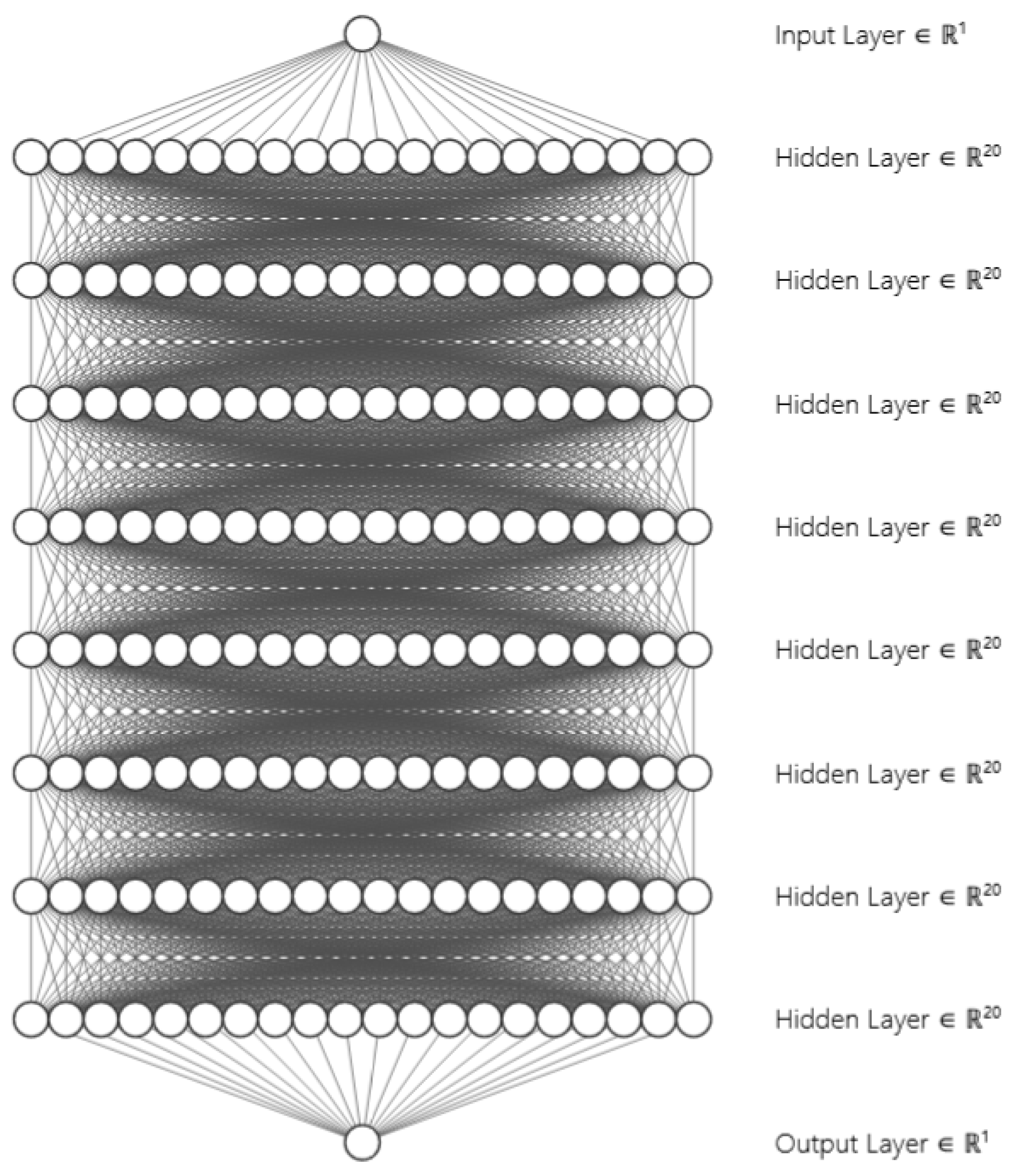
2.1. Feedforward Neural Networks
2.2. Cubic Splines
- 1.
- 2.
- 3.
- 4.
- 5.
- 6.
2.3. MARS
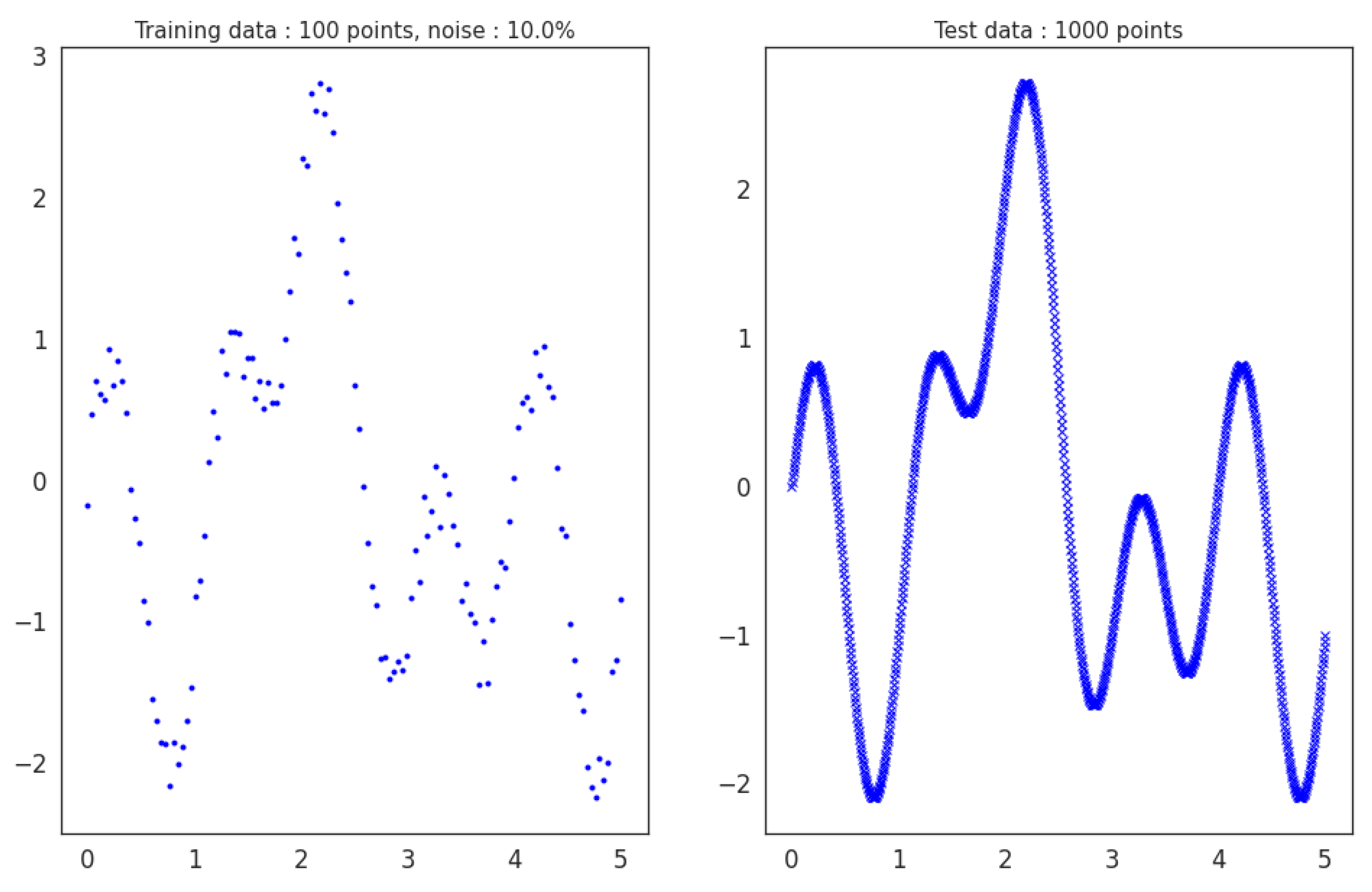
2.4. Producing Ground Truth, Sparse and Noisy Data
2.5. DNN Training Parameters
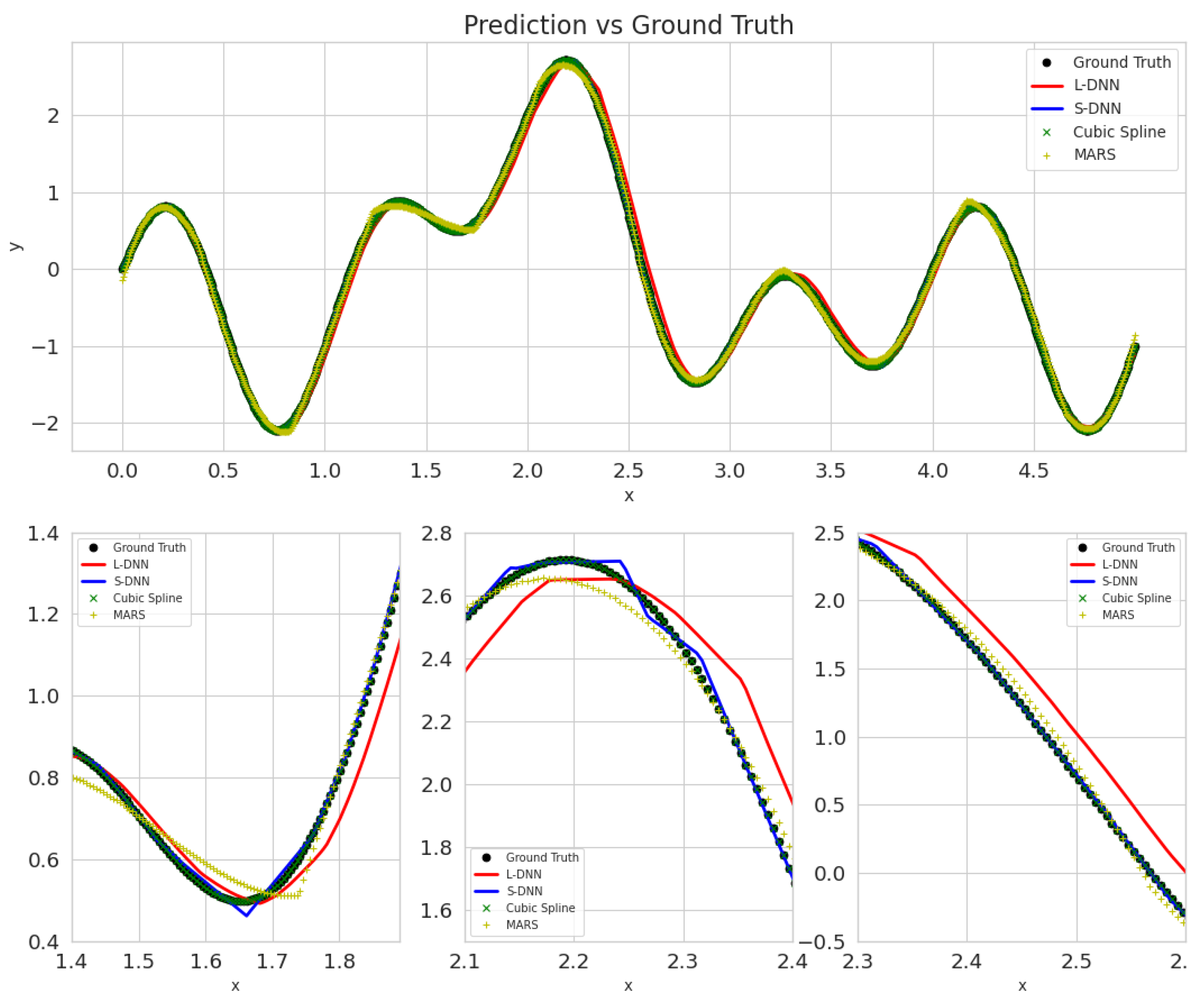
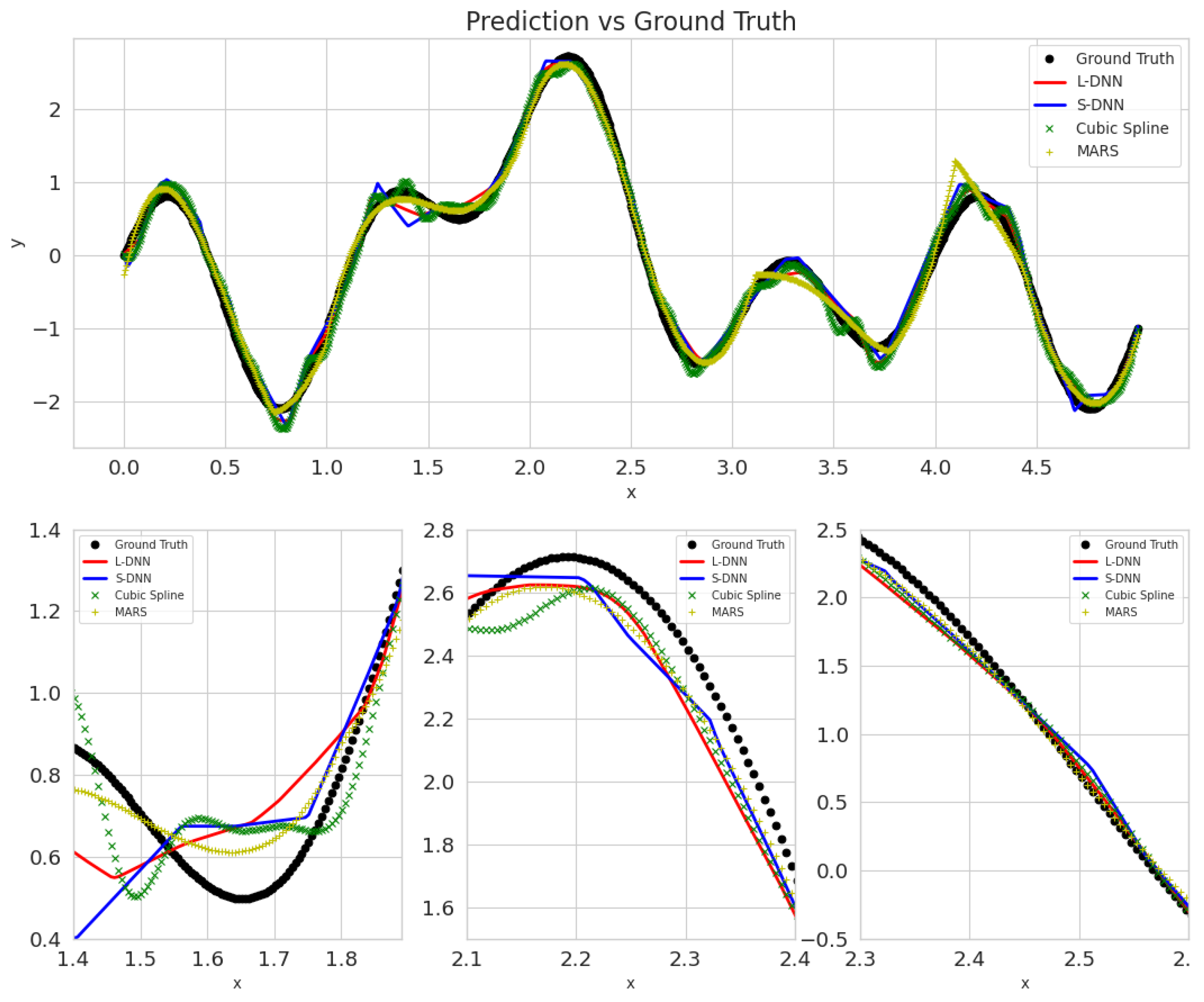
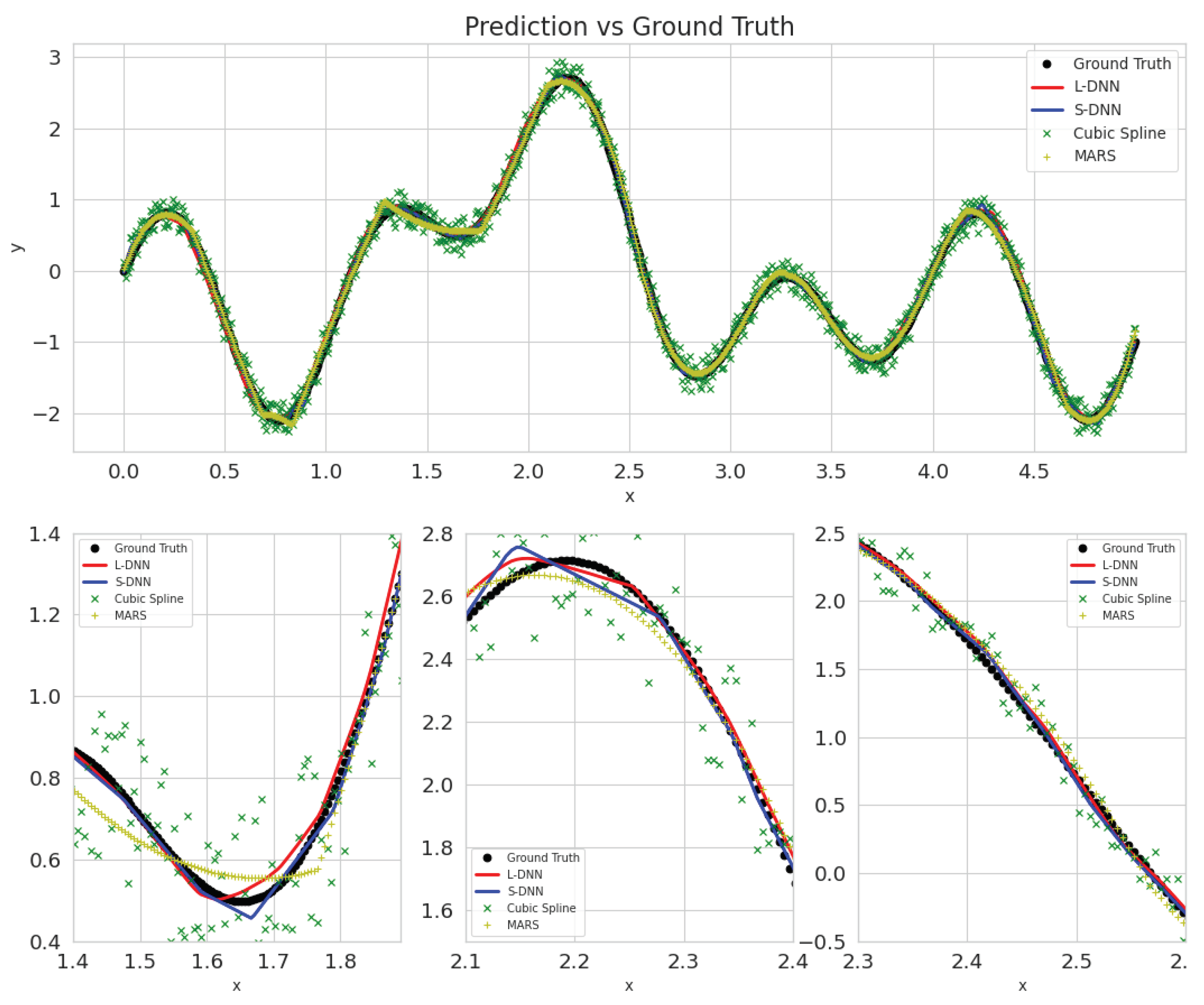
3. Results and Discussion
- SDNN.
- LDNN.
- MARS.
- Cubic Splines.
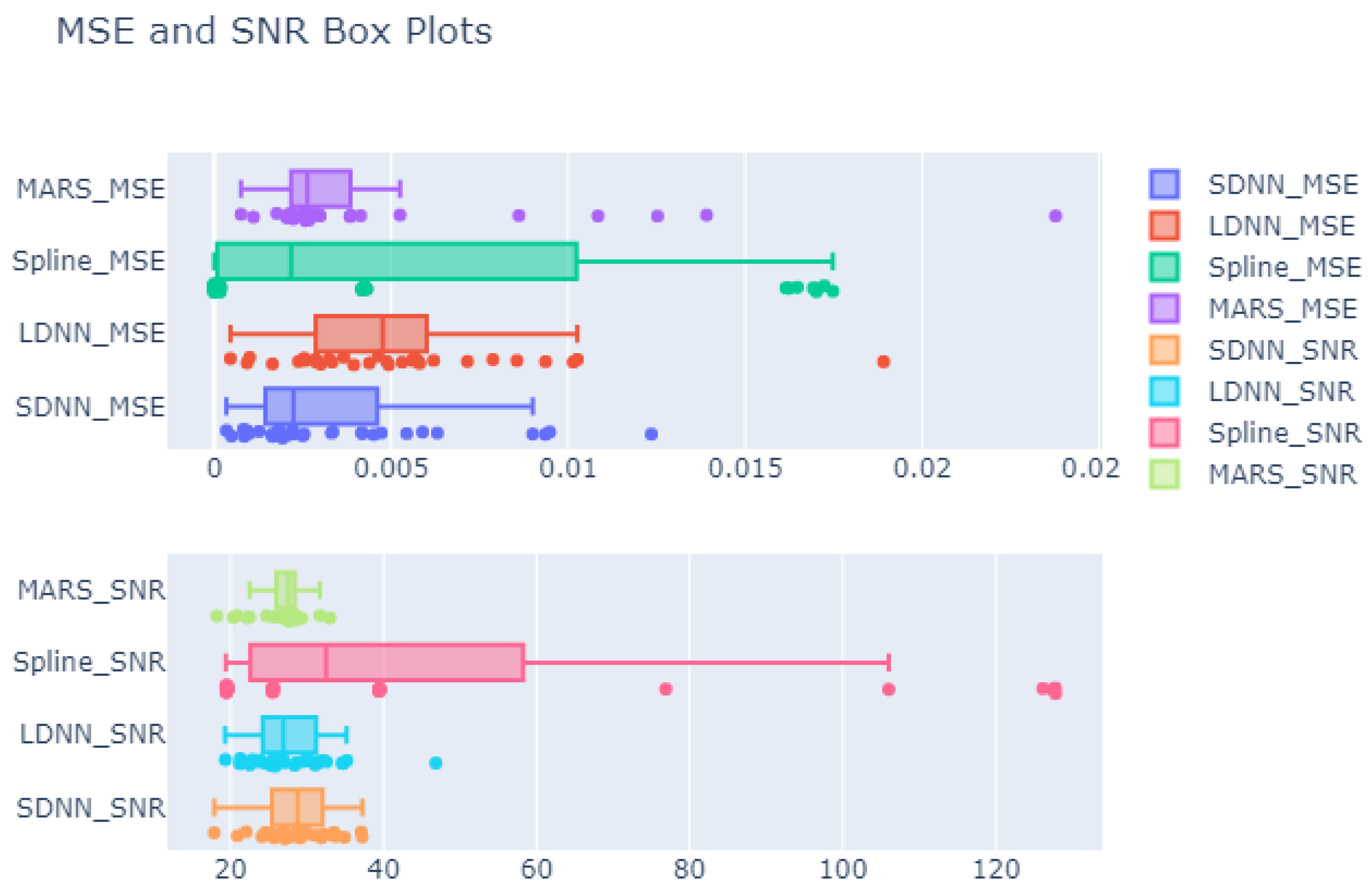
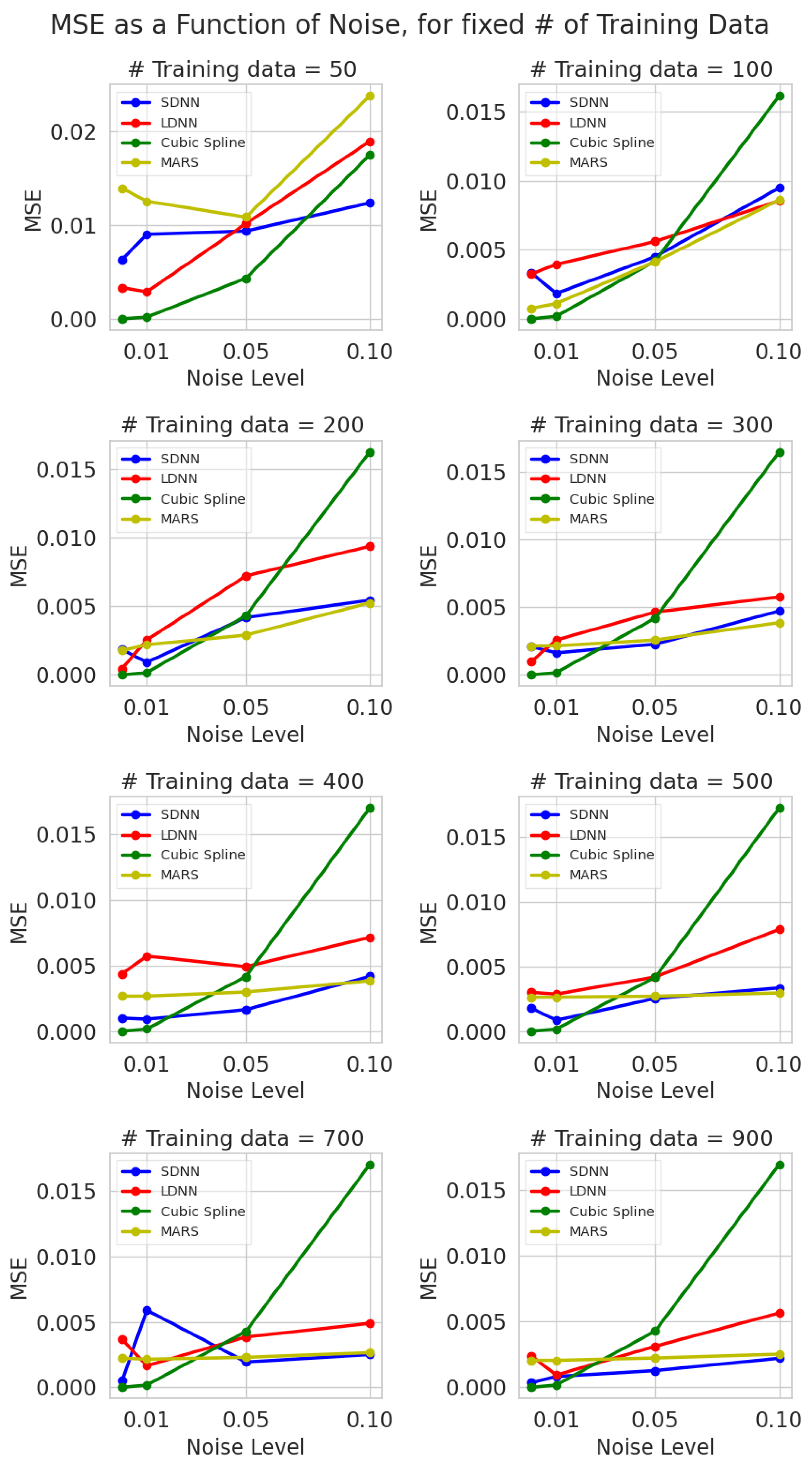
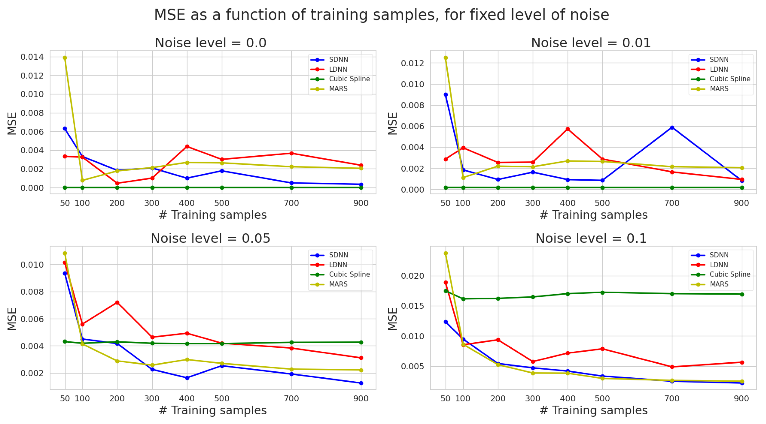
3.1. MSE
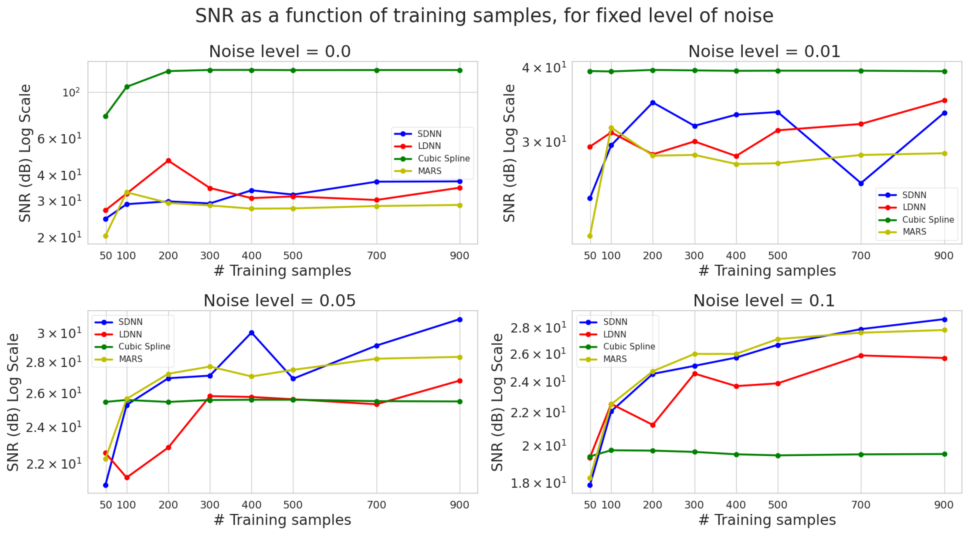
3.2. SNR
4. Conclusions
- ML methods (DNN and MARS) are significantly more robust to noise than cubic splines. As a result, they can discover the true function hidden under the noise, thus making ML a valuable tool in practical applications.
- Using more data reduces the effect of noise on the interpolation precision. Hence, noisy data should be best modelled using ML models instead of traditional methods, such as splines.
- Cubic splines provide precise interpolation when the data have low noise or are noiseless; they are inaccurate when data is noisy. Under noiseless conditions, splines consistently perform better, irrespective of the number of training samples used, since they are efficient even when data is sparse. Therefore, the cubic spline interpolation can significantly outperform ML models for sparse and noiseless data.
- DNN requires a complicated training procedure that is more time-consuming than splines and MARS. Moreover, DNN’s stochastic nature and sensitivity to hyperparameters increase the uncertainty until an optimal model is discovered. However, a good initialization coupled with an optimal hyperparameter set can provide convergence to a close-to-optimal solution.
- MARS models have the lowest variance regarding SNR, with noise affecting their SNR performance only slightly. Using more data alleviates this effect.
- The importance of initialization is more important for larger and deeper DNNs reflected in more unstable behaviour for LDNN rather than SDNN.
- SDNN exceeds LDNN performance. This is probably due to the over-parametrization of LDDN. Thus, LDNNs are more prone to overfitting the noise.
- Increasing the quantity of training data makes DNN a more attractive option. Further work, however, is required to understand the limitations of the DNN models.
- DNN’s low explainability remains problematic for engineering and medical applications. Thus, further work is required in this area as well.
Author Contributions
Funding
Data Availability Statement
Conflicts of Interest
Abbreviations
| NN | Neural network(s) |
| DNN | Deep neural network |
| FNN | Feedforward neural network |
| FFC | Feedforward fully connected |
| RNN | Recurrent neural network |
| CNN | Convolutional neural network |
| ReLU | Rectified linear unit |
| ELU | Exponential linear unit |
| GELU | Gaussian linear unit |
| BF | Basis function |
| MARS | Multivariate adaptive regression splines |
| GCV | Generalized cross-validation |
| SNR | Signal-to-noise ratio |
| MSE | Mean squared error |
Appendix A


References
- Zhu, L.; Zhang, W.; Kou, J.; Liu, Y. Machine learning methods for turbulence modeling in subsonic flows around airfoils. Phys. Fluids 2019, 31, 015105. [Google Scholar] [CrossRef]
- Duraisamy, K.; Iaccarino, G.; Xiao, H. Turbulence Modeling in the Age of Data. Annu. Rev. Fluid Mech. 2019, 51, 357–377. [Google Scholar] [CrossRef] [Green Version]
- Botu, V.; Ramprasad, R. Adaptive machine learning framework to accelerate ab initio molecular dynamics. Int. J. Quantum Chem. 2015, 115, 1074–1083. [Google Scholar] [CrossRef]
- Milano, M.; Koumoutsakos, P. Neural Network Modeling for Near Wall Turbulent Flow. J. Comput. Phys. 2002, 182, 1–26. [Google Scholar] [CrossRef] [Green Version]
- Crowell, A.R.; McNamara, J.J. Model Reduction of Computational Aerothermodynamics for Hypersonic Aerothermoelasticity. AIAA J. 2012, 50, 74–84. [Google Scholar] [CrossRef]
- Brouwer, K.R.; McNamara, J.J. Surrogate-based aeroelastic loads prediction in the presence of shock-induced separation. J. Fluids Struct. 2020, 93, 102838. [Google Scholar] [CrossRef]
- Deshmukh, R.; McNamara, J.J. Reduced Order Modeling of a Flow Past a Cylinder using Sparse Coding. In Proceedings of the 55th AIAA Aerospace Sciences Meeting, Grapevine, TX, USA, 9–13 January 2017. [Google Scholar] [CrossRef]
- Ritos, K.; Drikakis, D.; Kokkinakis, I.W.; Spottswood, S.M. Computational aeroacoustics beneath high speed transitional and turbulent boundary layers. Comput. Fluids 2020, 203, 104520. [Google Scholar] [CrossRef] [Green Version]
- Frank, M.; Drikakis, D.; Charissis, V. Machine-Learning Methods for Computational Science and Engineering. Computation 2020, 8, 15. [Google Scholar] [CrossRef] [Green Version]
- Chou, S.M.; Lee, T.S.; Shao, Y.E.; Chen, I.F. Mining the breast cancer pattern using artificial neural networks and multivariate adaptive regression splines. Expert Syst. Appl. 2004, 27, 133–142. [Google Scholar] [CrossRef]
- Adamowski, J.; Chan, H.F.; Prasher, S.O.; Sharda, V.N. Comparison of multivariate adaptive regression splines with coupled wavelet transform artificial neural networks for runoff forecasting in Himalayan micro-watersheds with limited data. J. Hydroinform. 2011, 14, 731–744. [Google Scholar] [CrossRef]
- Lu, C.J.; Lee, T.S.; Lian, C.M. Sales forecasting for computer wholesalers: A comparison of multivariate adaptive regression splines and artificial neural networks. Decis. Support Syst. 2012, 54, 584–596. [Google Scholar] [CrossRef]
- Lin, C.J.; Chen, H.F.; Lee, T.S. Forecasting Tourism Demand Using Time Series, Artificial Neural Networks and Multivariate Adaptive Regression Splines:Evidence from Taiwan. Int. J. Bus. Adm. 2011, 2, 14–24. [Google Scholar] [CrossRef] [Green Version]
- Enjilela, E.; Lee, T.Y.; Wisenberg, G.; Teefy, P.; Bagur, R.; Islam, A.; Hsieh, J.; So, A. Cubic-Spline Interpolation for Sparse-View CT Image Reconstruction With Filtered Backprojection in Dynamic Myocardial Perfusion Imaging. Tomography 2019, 5, 300–307. [Google Scholar] [CrossRef]
- da Silva, S.; Paixão, J.; Rébillat, M.; Mechbal, N. Extrapolation of AR models using cubic splines for damage progression evaluation in composite structures. J. Intell. Mater. Syst. Struct. 2021, 32, 284–295. [Google Scholar] [CrossRef]
- Sobester, A.; Keane, A. Airfoil Design via Cubic Splines - Ferguson’s Curves Revisited. In Proceedings of the Collection of Technical Papers-2007 AIAA InfoTech at Aerospace Conference, Rohnert Park, CA, USA, 7–10 May 2007; Volume 2. [Google Scholar] [CrossRef] [Green Version]
- Nieto, F. Radar track segmentation with cubic splines for collision risk models in high density terminal areas. J. Aerosp. Eng. 2014, 229, 1371–1383. [Google Scholar] [CrossRef] [Green Version]
- Fukushima, K. Cognitron: A self-organizing multilayered neural network. Biol. Cybern. 1975, 20, 121–136. [Google Scholar] [CrossRef]
- Unser, M. A Representer Theorem for Deep Neural Networks. J. Mach. Learn. Res. 2019, 20, 1–30. [Google Scholar]
- Parhi, R.; Nowak, R.D. The Role of Neural Network Activation Functions. IEEE Signal Process. Lett. 2020, 27, 1779–1783. [Google Scholar] [CrossRef]
- Parhi, R.; Nowak, R.D. What Kinds of Functions Do Deep Neural Networks Learn? Insights from Variational Spline Theory. SIAM J. Math. Data Sci. 2022, 4, 464–489. [Google Scholar] [CrossRef]
- Balestriero, R.; Baraniuk, R. A Spline Theory of Deep Learning. In Proceedings of the 35th International Conference on Machine Learning, Stockholm, Sweden, 10–15 July 2018; pp. 374–383. [Google Scholar]
- Daub, D.; Willems, S.; Gülhan, A. Experiments on aerothermoelastic fluid–structure interaction in hypersonic flow. J. Sound Vib. 2022, 531, 116714. [Google Scholar] [CrossRef]
- Spottswood, S.M.; Beberniss, T.J.; Eason, T.G.; Perez, R.A.; Donbar, J.M.; Ehrhardt, D.A.; Riley, Z.B. Exploring the response of a thin, flexible panel to shock-turbulent boundary-layer interactions. J. Sound Vib. 2019, 443, 74–89. [Google Scholar] [CrossRef]
- Brouwer, K.R.; Perez, R.A.; Beberniss, T.J.; Spottswood, S.M.; Ehrhardt, D.A. Experiments on a Thin Panel Excited by Turbulent Flow and Shock/Boundary-Layer Interactions. AIAA J. 2021, 59, 2737–2752. [Google Scholar] [CrossRef]
- Kokkinakis, I.; Drikakis, D.; Ritos, K.; Spottswood, S.M. Direct numerical simulation of supersonic flow and acoustics over a compression ramp. Phys. Fluids 2020, 32, 066107. [Google Scholar] [CrossRef]
- Mhaskar, H.N.; Liao, Q.; Poggio, T.A. Learning Real and Boolean Functions: When Is Deep Better Than Shallow. arXiv 2016, arXiv:1603.00988. [Google Scholar]
- Moore, B.; Poggio, T.A. Representation properties of multilayer feedforward networks. Neural Netw. 1988, 1, 203. [Google Scholar] [CrossRef]
- Maas, A.L. Rectifier Nonlinearities Improve Neural Network Acoustic Models. In Proceedings of the 30th International Conference on Machine Learning, Atlanta, GA, USA, 16–21 June 2013; Volume 28. [Google Scholar]
- Trottier, L.; Giguère, P.; Chaib-draa, B. Parametric Exponential Linear Unit for Deep Convolutional Neural Networks. arXiv 2016, arXiv:1605.09332. [Google Scholar]
- Hendrycks, D.; Gimpel, K. Bridging Nonlinearities and Stochastic Regularizers with Gaussian Error Linear Units. arXiv 2016, arXiv:1606.08415. [Google Scholar]
- Wegman, E.J.; Wright, I.W. Splines in Statistics. J. Am. Stat. Assoc. 1983, 78, 351–365. [Google Scholar] [CrossRef]
- Friedman, J.H. Multivariate Adaptive Regression Splines. Ann. Stat. 1991, 19, 1–67. [Google Scholar] [CrossRef]
- Golub, G.H.; Heath, M.; Wahba, G. Generalized Cross-Validation as a Method for Choosing a Good Ridge Parameter. Technometrics 1979, 21, 215–223. [Google Scholar] [CrossRef]
- Rumelhart, D.E.; Hinton, G.E.; Williams, R.J. Learning representations by back-propagating errors. Nature 1986, 323, 533–536. [Google Scholar] [CrossRef]
- Kingma, D.P.; Ba, J. Adam: A Method for Stochastic Optimization. arXiv 2014, arXiv:1412.6980. [Google Scholar]
- Jin, C.; Ge, R.; Netrapalli, P.; Kakade, S.M.; Jordan, M.I. How to Escape Saddle Points Efficiently. arXiv 2017, arXiv:1703.00887. [Google Scholar]
- Shalev-Shwartz, S.; Shamir, O.; Shammah, S. Failures of Deep Learning. arXiv 2017, arXiv:1703.07950. [Google Scholar]
- Skorski, M. Revisiting Initialization of Neural Networks. arXiv 2020, arXiv:2004.09506. [Google Scholar]


| - | Layer1 | Layer2 | Layer3 | Layer4 | Layer5 | Layer6 | Layer7 | Layer8 | Final Layer |
|---|---|---|---|---|---|---|---|---|---|
| Neurons | 500 | 1000 | 2000 | 5000 | 2000 | 1000 | 500 | 20 | 1 |
| Optimizer | Learning Rate | Epochs | Learning Rate Decay |
|---|---|---|---|
| Adam | 0.3 | 6000 | yes |
| Adamax | 0.03 | 7000 | no |
| Adadelta | 0.01 | 15,000 | - |
| SGD | 0.003 | 25,000 | - |
| RMSprop | - | 30,000 | - |
| Nadam | - | - | - |
| LBFGS | - | - | - |
Disclaimer/Publisher’s Note: The statements, opinions and data contained in all publications are solely those of the individual author(s) and contributor(s) and not of MDPI and/or the editor(s). MDPI and/or the editor(s) disclaim responsibility for any injury to people or property resulting from any ideas, methods, instructions or products referred to in the content. |
© 2023 by the authors. Licensee MDPI, Basel, Switzerland. This article is an open access article distributed under the terms and conditions of the Creative Commons Attribution (CC BY) license (https://creativecommons.org/licenses/by/4.0/).
Share and Cite
Poulinakis, K.; Drikakis, D.; Kokkinakis, I.W.; Spottswood, S.M. Machine-Learning Methods on Noisy and Sparse Data. Mathematics 2023, 11, 236. https://doi.org/10.3390/math11010236
Poulinakis K, Drikakis D, Kokkinakis IW, Spottswood SM. Machine-Learning Methods on Noisy and Sparse Data. Mathematics. 2023; 11(1):236. https://doi.org/10.3390/math11010236
Chicago/Turabian StylePoulinakis, Konstantinos, Dimitris Drikakis, Ioannis W. Kokkinakis, and Stephen Michael Spottswood. 2023. "Machine-Learning Methods on Noisy and Sparse Data" Mathematics 11, no. 1: 236. https://doi.org/10.3390/math11010236