A Combined Model Based on Recurrent Neural Networks and Graph Convolutional Networks for Financial Time Series Forecasting

Abstract

Accurate and real-time forecasting of the price of oil plays an important role in the world economy. Research interest in forecasting this type of time series has increased considerably in recent decades, since, due to the characteristics of the time series, it was a complicated task with inaccurate results. Concretely, deep learning models such as Convolutional Neural Networks (CNNs) and Recurrent Neural Networks (RNNs) have appeared in this field with promising results compared to traditional approaches. To improve the performance of existing networks in time series forecasting, in this work two types of neural networks are brought together, combining the characteristics of a Graph Convolutional Network (GCN) and a Bidirectional Long Short-Term Memory (BiLSTM) network. This is a novel evolution that improves existing results in the literature and provides new possibilities in the analysis of time series. The results confirm a better performance of the combined BiLSTM-GCN approach compared to the BiLSTM and GCN models separately, as well as to the traditional models, with a lower error in all the error metrics used: the Root Mean Squared Error (RMSE), the Mean Squared Error (MSE), the Mean Absolute Percentage Error (MAPE) and the R-squared (R²). These results represent a smaller difference between the result returned by the model and the real value and, therefore, a greater precision in the predictions of this model.

1. Introduction

In the 1970s, the Box–Jenkins [1] approaches became popular for time series forecasting, introducing AutoRegressive Integrated Moving Average (ARIMA) models and their variants as the main time series forecasting tools. However, machine learning models based on Deep Neural Networks (DNNs), that is, networks with multiple layers, have been developed in recent decades. In particular, those based on Recurrent Neural Networks (RNNs) such as Long Short-Term Memory (LSTM), since they have the ability to carry the memory of past states. RNNs derive from feed-forward neural networks, and early research was based on time series predictions including Kamijo and Tanigawa [2], Chakraborty et al. [3] and a comparison with the ARIMA models of Kohzadi et al. [4].

Forecasting the prices of commodities has been a challenge in the literature, full of volatility, uncertainty and complexity, that has led researchers to seek the most accurate and efficient methodologies available to try to respond to the need to make predictions in the future. In this context, RNNs are becoming competitive forecasting methods with the potential to replace classical statistical techniques such as Exponential Smoothing (ETS) and ARIMA, which are popular for their high accuracy and efficiency. However, unlike these techniques, RNNs need little information about the data contained in the time series, allowing their application to a wide range of problems, as one can see in Kolarik and Rudorfer [5].

The use of DNNs for time series forecasting is based exclusively on observed data. Since feed-forward networks are universal approximators, as in Hornik et al. [6], an artificial neural network has the power to model any kind of time series. The ability to generalize allows these networks to learn even with noisy or missing data, and they are even capable of representing nonlinear time series.

The application of LSTM networks for the prediction of time series is widely studied in the literature [7,8,9,10,11,12]. Pirani et al. [13] incorporated into the literature a comparison that includes the BiLSTM model in the prediction of time series, with an analysis especially focused on analyzing the behavior of the BiLSTM, ARIMA, Gated Recurrent Unit (GRU) and LSTM models. Nevertheless, the application of Graph Convolutional Networks (GCNs) in many fields extends to time series [14], showing that GCNs are effective in taking advantage of correlations between nodes, and thus representing time series in terms of graphs where the different observations become nodes of this [15].

Below are the most studied approaches for time series forecasting in general, and for financial forecasting [13,16] and commodity analysis in particular [4]. Thus, this section focuses on Artificial Neural Networks (ANNs) with special interest in LSTM, BiLSTM and GCNs. Finally, traditional and recent approaches to commodity analysis are also presented.

1.1. Artificial Neural Networks for Time Series Forecasting

More and more data are becoming available, making ANNs an increasingly dominant technique for machine learning tasks. There is an extensive literature on the use of ANNs in prediction tasks. Zhang et al. [17] make an extensive summary of works in which neural networks have been applied. According to the authors, ANNs have several characteristics that make them suitable for prediction tasks compared to traditional statistical techniques.

Tan et al. [18] stated that economic time series are characterized by their nonlinear, dynamic and chaotic behavior, a fact that has attracted the attention of many researchers in recent decades and has driven the development of new models for their prediction.

One of the main advantages of ANNs is their ability to create associations between data even when they do not consist of a direct correlation; this feature allows generalizing the data and making predictions from these relationships, especially when it comes to nonlinear relationships [6]. This makes deep learning the most widely used technique compared to traditional techniques.

In the increasingly demanding time series forecasting tasks, the use of DNNs has spread exponentially. Through a combination of an ARIMA and ANN model, Zhang [19] sought to use the advantages of both methodologies to solve this type of problem. To carry out these tests, he used real time series, with results that improved those of ARIMA and ANN separately.

In the same line of research, Hill et al. [20] studied the behavior of ANNs in comparison with forecasts of six statistical methods for time series [21], pointing out a better performance of neural networks compared to traditional methods, being particularly more effective for discontinuous time series, while Gheyas and Smith [22] proposed a simple approach for forecasting univariate time series, based on a set of generalized regression learning techniques. Khashei and Bijari [23] complete the existing literature with their studies using a novel model that combines traditional statistical techniques and ANNs, obtaining empirical results showing that it is an effective way to improve the accuracy of time series forecasting.

To improve the possible existing problems with time series with linear and nonlinear components, Yolcu et al. [24] developed a hybrid model consisting of linear and nonlinear structures, assuming that the time series can have both components, with results that show greater efficiency than the results reported in the available literature.

Determining the optimal structure of the network and the training method for a given problem is crucial in order to obtain maximum precision with an ANN. Zhang and Kline [25] included the choice of input variables in the model as another critical factor.

1.1.1. Long Short-Term Memory

In the model proposed by Hochreiter and Schmidhuber [26], a Long-Short Term Memory (LSTM) network has the ability to store information from iterations in the network; this storage behaves as previous states that can be accessed so that the network can perform the calculation of the next state.

As we have already pointed out, the application of LSTM networks for time series forecasting is widely studied in the literature. An LSTM-type network was used by Gers et al. [27] to make predictions. Malhotra et al. [8] studied whether LSTM networks have the ability to detect alterations in time series, while a new adaptive gradient method for RNNs was used by Guo et al. [11], allowing stronger predictions even on data with outliers. Cinar et al. [9] proposed, with the objective of capturing periods and modeling missing values in the time series, an extended attention mechanism. Laptev et al. [10] discovered that neural networks could be more efficient than traditional methods when dealing with time series with high correlation and a large number of observations.

This type of network has the ability to model temporal dependencies over longer horizons without neglecting short-term patterns [12].

1.1.2. Bidirectional LSTM

Bidirectional LSTM networks, known as BiLSTM, differ from the existing model in that they allow double training since the inputs are processed twice, from left to right and then from right to left.

In their research, Siami-Namini et al. [28] tried to explore to what extent it is beneficial to add additional layers for model training, obtaining as a result that the BiLSTM model offered better results than the regular predictions of an LSTM network. The results coincide with the conclusions obtained by Kim and Moon [29] in their work, in which, through a neural network, they made predictions from a time series of the trading area. Yang and Wand [30] achieved similar results by comparing financial time series prediction with a BiLSTM, Support Vector Regression (SVR) and ARIMA network.

1.1.3. Graph Convolutional Networks

Graph Convolutional Networks (GCNs) are a type of data structure that provides a model for a set of nodes and their edges, representing objects and their relationships. Indeed, GCNs are considered as a form of generalized Graph Neural Network (GNN) for graph-structured data. The existing literature on GCNs is developing at great speed due to the great power to represent graph systems; they are used to denote a large number of relationships in different areas [31]. The research carried out covers a large number of specializations such as social networks [32] and physics [33], among others. The study of GCNs focuses on tasks such as node classification, node link predictions and node clustering.

Neural networks were first applied to acyclic graphs by Sperduti and Starita [34], providing the first studies on GNNs. These neural networks were initially investigated by Gori et al. [35] and subsequently Scarselli et al. [36] and Gallicchio et al. [37] went deeper into the research. These early GNN models learn the destination nodes by iteratively propagating the neighboring nodes until a stable point is found [38].

GNNs are useful for processing data that can be represented as graphs. For that reason, time series modeling has become a research topic among GNN developers and researchers in various fields such as economics, finance, energy, etc. In their research, Wu et al. [39] propose a general GNN framework with a specific design for time series, automatically extracting the relationships between various variables through a graph-learning module. Deng and Hooi [40] carried out studies on the detection of unexpected events during the prediction of time series, based on a model that combines GNNs and weight assignment that allows explaining those anomalies that have been detected, with results that improved the existing literature and modeled the relationships of the variables with high precision. Recently, the use of GNNs in the different research fields was reviewed by Jian and Luo [41], with special attention to traffic prediction.

In the research carried out by Wang et al. [42], they reflected how the components and relationships of financial data can be represented as graphs since they allow reflection of both individual characteristics and more complex relationships. The complexity and volatility associated with economic time series often result in a heterogeneous or variable graph, which is a challenge for graph neural networks.

There are few works in the literature that combine the use of GCNs and BiLSTM networks in the prediction of time series, as in that of Ma et al. [43] who, based on a combined model, predicted the flow of subway passengers. Specifically, in that work a GCN is first applied to capture the spatial correlation features and then BiLSTM is applied to capture the time-dependent features. Finally, the output is fused through a full connection layer. However, the strategy proposed in this work differs from that approach, as we will see in Section 3. Along the same lines, Wu et al. [44] carried out their research with GCN and LSTM models for traffic prediction, research similar to that carried out by Li et al. [45]. This combined model has been implemented in this work for comparative purposes.

To the best of our knowledge, there is little research in the economic and financial field combining DNN models such as the one proposed in this work.

1.2. Commodity Analysis

Forecasting commodity values from time series is a critical task in many disciplines including finance, planning and decision-making. Precious metals tend to have higher prices due to their rarity or difficulty in acquiring them. In ancient times, some precious metals were used as currency, and today they are used as financial and industrial products. Hence, it is important to be able to make price predictions as accurately as possible, based on previously acquired values and with importance on those economic factors such as production, circulation and demand that may influence the data [46].

The prediction of economic values represents a classic but challenging problem, which attracted the attention of economist researchers and engineers with the common purpose of building efficient prediction models and exploring machine learning tools in recent decades, being studied by different researchers such as Jiang [47].

The classic statistical methods used in econometrics continue to be used in different economic and financial applications, such as by Almasarweh and Alwadi [48] and Chung et al. [49], who, based on an ARIMA model and based on data on banking values of Chinese industry, made predictions about these values.

In the literature, it is possible to find other methodologies for the analysis of time series, such as Autoregressive Fractionally Integrated Moving Average (ARFIMA) [50,51], Support Vector Machine (SVM) [52] and Generalized AutoRegressive Conditional Heteroscedasticity (GARCH) [53].

With the advance of technologies, ANNs were hybridized with the ARIMA model in order to obtain more accurate results, explaining that this type of technique has the ability to predict commodity prices more accurately than other methods. Research conducted by Ghezelbash [54] used a Multilayer Perceptron (MLP) to perform prediction of changes in stock prices and gold prices from data obtained from the Tehran Stock Exchange (TSE), showing that ANNs provide a more sophisticated and nonlinear approach and that ANN models perform better than traditional statistical techniques, requiring minimal feature engineering compared to other methods. Dehghani [55] applied ANN algorithms to predict copper price volatility, obtaining that the performance is superior to classical estimation methods. The research conducted by Malliaris and Malliaris [56] by using ANNs allowed them to perform the prediction of gold, oil and euro prices. For the prediction of prices and possible super cycles of raw materials, Monge and Lazcano [57] combined the analysis of an ARFIMA model together with the prediction produced by ANNs. Finally, Liu et al. [58] proposed a regularization regression model for precious metal price prediction, in particular by using a hybrid model between CNN and LSTM.

All in all, and considering the potential of LSTM and GCNs separately, this work proposes a DNN model that properly combines LSTM and BiLSTM with a GCN for the analysis of time series of the market values of commodities, and establishes a comparison with RNNs and traditional statistical models through the metrics obtained. The BiLSTM-GCN model represents an evolution of the models existing up to now and is described in the next sections, capturing the characteristics that make both models accurate time series forecasting techniques. What makes the BiLSTM-GCN model a novel and effective tool in time series forecasting is the use of graph convolutional networks for time series forecasting, applied in combination with a BiLSTM-type network to achieve optimal results justified by the existing literature.

The main contributions of this research can be summarized in the following points:

-

Review of main statistical techniques for forecasting economic time series.

-

Creation of a new hybrid model that combines recurrent and graph convolutional networks.

-

Demonstration of an improvement in the results reflected in the existing literature provided by the new model.

-

Comparison of the main models used in the prediction of time series.

The rest of the paper is organized as follows: Section 2 provides a detailed description of the proposed model and its architecture. The experiments developed for the evaluation of the network and the results obtained are specified in Section 3. The discussion of the results is presented in Section 4. Finally, Section 5 is dedicated to describing the main conclusions and the future lines of research of this work.

2. Methodology

2.1. ANN Architecture

One of the main characteristics of neural networks is the ability to store neurons in different layer levels; the different levels that can be found in an ANN are the input layer, hidden layers and an output layer [59]. In the architecture of an ANN, special consideration must be given to how many neurons will make up each layer, the parameters set for training the network and the metrics that will allow the behavior and resolution of the neural network to be evaluated.

The signals from the outside will be received by the input layers, which will be responsible for propagating the information to the following layers. In the hidden layers, the neurons will be in charge of processing the data received from the previous layer. The output layer, located last, will be responsible for responding to each of the inputs [60]. Güler and Übeyli [61] determined how the most efficient methodology for choosing the appropriate number of layers is the one that combines trial and error.

A neural network is usually represented as follows:

$$I-\left(N_1, N_2, N_3, \dots , N_m\right)-O$$

(1)

I is the representation of the number of inputs, while N_m defines the number of neurons that are part of the hidden layer m and the output layer O.

Fu [62] described how, in each layer, the neurons are connected with the neurons that are in the next one; these relationships between neurons have an associated weight that is calculated based on the result obtained after the calculations and the real result that is expected. The error is propagated to the previous layers, which allows an adjustment of the connection weights throughout the training.

To carry out this process, it is necessary to have a second set of data that allow the validation to be carried out, and from this second set of data accuracy of the model based on the Mean Square Error (MSE) can be evaluated, trying to reduce this value.

A neural network is structured as follows: the input vector is represented by $Y_i=\left\{y_1, y_2, y_3, \dots , y_n\right\};$the vector associated with the weights between the neurons from the i neurons of the first layer connected with the n neurons found in the first hidden layer is denoted as $W_{jk}\left(j\in \mathbb{N};k\in \mathbb{N}\right);$the vector that corresponds to the n neurons that make up the hidden layers $X_k\left(k=1, 2, 3, \dots , m\right)$ is denoted as $X_k=f\left({\displaystyle \sum }_{j=1}^n{W}_{jk}{Y}_j+{\mathsf{\Theta }}_k\right)$.

The vector from the output layer with a single neuron Y is $Y=f\left({\displaystyle \sum }_{k=1}^n{W}_k{X}_k+\mathsf{\Theta }\right)$. Finally, the polarized value of the neurons that make up the hidden layer is defined by ${\mathsf{\Theta }}_k\left(k=1, 2, 3, \dots , k\right)$and Θ is the polarized value of the hidden layer.

Hinton and Salakhutdinov [63] proposed to train neural networks from a correct initialization of weights and a certain number of deep layers instead of establishing random values as was the method until then. To carry out this process, an unsupervised training is carried out, later carrying it out in a supervised way, establishing the results obtained as initial weights.

Glorot and Bengio [64] established the initial values of the Xabier weights, an efficient option that allows initializing weights and avoiding supervised training. This scheme has become a standard deep learning methodology since it has shown improved performance and accuracy thanks to the choice of a nonlinear activation function, the most suitable being the Rectified Linear Unit (ReLU) studied by Jarrett et al. [65] and Nair and Hinton [66].

2.2. BiLSTM-GCN Network

The architecture of the network proposed in this work to carry out the prediction of crude oil prices (or predictions of any other type of time series independent of its characteristics) is made up of different stages, among which are included the collection and pre-processing of the data, the training of the BiLSTM-GCN combined scheme and the subsequent evaluation of the results obtained.

The transformations carried out for data processing consist of dividing the time series into training and validation sets, the first helping the network to learn the relationships between the data and the second allowing the efficiency of the model to be verified. Once the division is carried out, the data are normalized to values between 0 and 1 to avoid possible differences between scales.

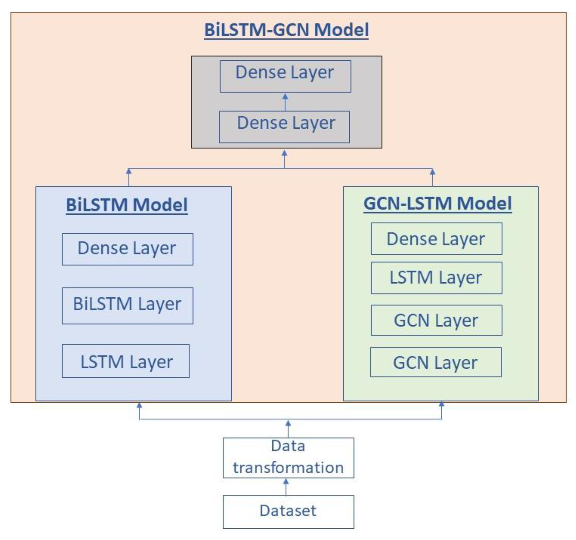
The BiLSTM-GCN combined scheme is composed of two pre-trained models with the time series belonging to the price of oil from which a prediction is obtained. Subsequently, a new model is generated with the outputs resulting from the previous ones, which receives as input again the time series and, after training, it makes the prediction as can be seen in Figure 1.

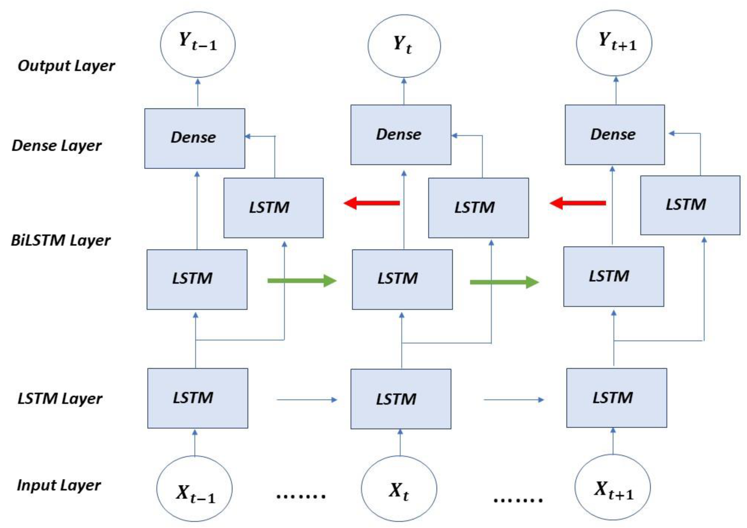
The first model that makes up the proposed network and corresponds to the BiLSTM part consists of an input layer, hidden layers and an output layer. The hidden layers with the concatenation of an LSTM layer, a BiLSTM layer and a dense layer that lead to the dense output layer are as shown in Figure 2. The data goes through the network in one direction, the one indicated by the green arrow, to later go through the network in the opposite direction, following the red arrows; the results flow into the dense output layer.

BiLSTM models are a variant of the simple LSTM architectures that allow for additional training by having the data traverse the input twice, firstly from left to right and then from right to left. The architecture that defines a BiLSTM model can be described by the following formulae:

$$h_t=f\left(w_1{x}_t+w_2{h}_{t-1}\right)$$

(2)

$${h_t}^{\prime }=f\left(w_3{x}_t+w_5{h}_{t+1}\right)$$

(3)

$$o_t=g\left(w_4{h}_4+w_6{h}_t\right)$$

(4)

x represents the inputs of the model, which will be modified by the weights w of the neurons that make up each h_t layer, resulting in the output h_t in the backward layer and the output of the forward layer h_t′, which when combined and after applying the activation function provide the output o_t.

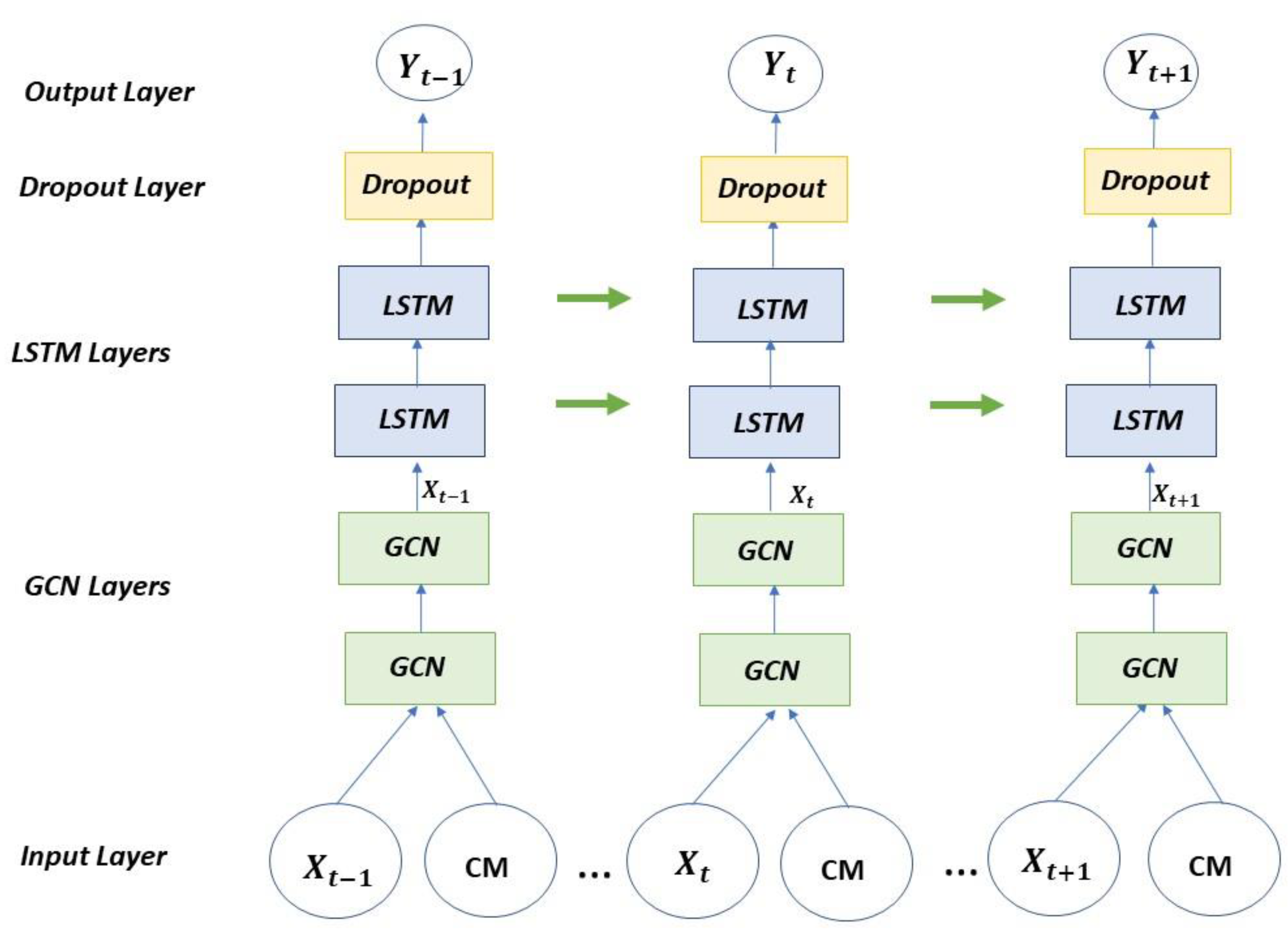
The second model is formed by a GCN-LSTM architecture inspired by the model developed by Zhao et al. [67] from the StellarGraph library, which consists of two parts: a set of graph convolutional layers defined by the user and a set of specified LSTM layers, and finally a dropout layer and a dense layer for performance improvement.

In order to apply mathematical formulations to a GCN, Jiang and Luo [41] introduced the following notations. D is defined as the matrix of graphs, in which each of the elements is $D_{ii}=\Vert N\left(v_i\right)\Vert .$The nodes are denoted as $v_i\in V,$where V is the set of vertices or nodes. The neighbors of a node v are defined as $N\left(v\right)=\left\{u\in V|\left(v,u\right)\in E\right\}$, where E is the set of edges.

This model receives as inputs the time series and a Correlation Matrix (CM) resulting from the generation of the graph from the time series as specified in Figure 3.

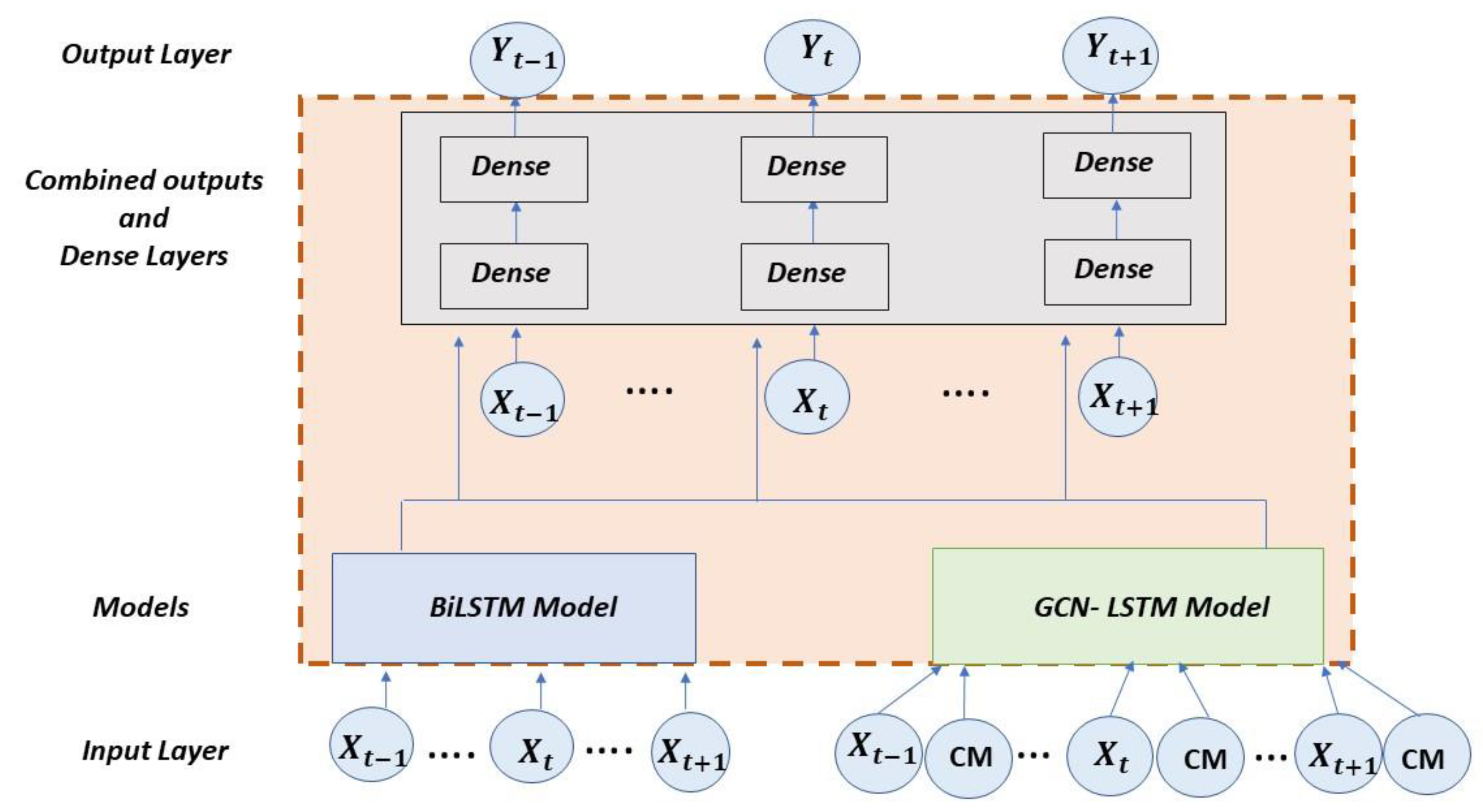
The combined proposed architecture is formed by concatenating the outputs of the aforementioned models after being pre-trained and joining them in a new network in which the time series to be studied is introduced again (see Figure 4). This hybrid model is also composed of two dense layers in addition to the output layer. The concatenation of DNN models allows taking advantage of the capacity of each type of network to make more precise predictions [68,69]. For the creation of the hybrid model, the outputs obtained from the GCN-LSTM and BiLSTM models are added and, as part of the new network, two dense layers are then added to improve the processing of the network. The resulting combined model is named BiLSTM-GCN in this work.

3. Results

3.1. Data Description

In this section, the data used in the evaluation process of our proposal will be described. The time series corresponding to the West Texas Intermediate (WTI) crude oil price index obtained from Thomson Eikon Reuters with a daily timeframe with data from 10 January 1983 to 15 June 2022 was obtained. WTI is the spot price of West Texas Intermediate grade oil; it is, along with the spot price of Brent, one of the main benchmarks used to set the price of oil.

For this work, 10,289 observations were obtained, which were loaded into a dataframe generated with the Pandas library in Python for processing. Using this library allowed us to load the time series data into a table that served as input to the neural network. Once the data were structured in the dataframe, selecting the date field of the time series as the index of the table, a transformation was made to a graph of nodes using the Visibility Graph method developed by Lacasa et al. 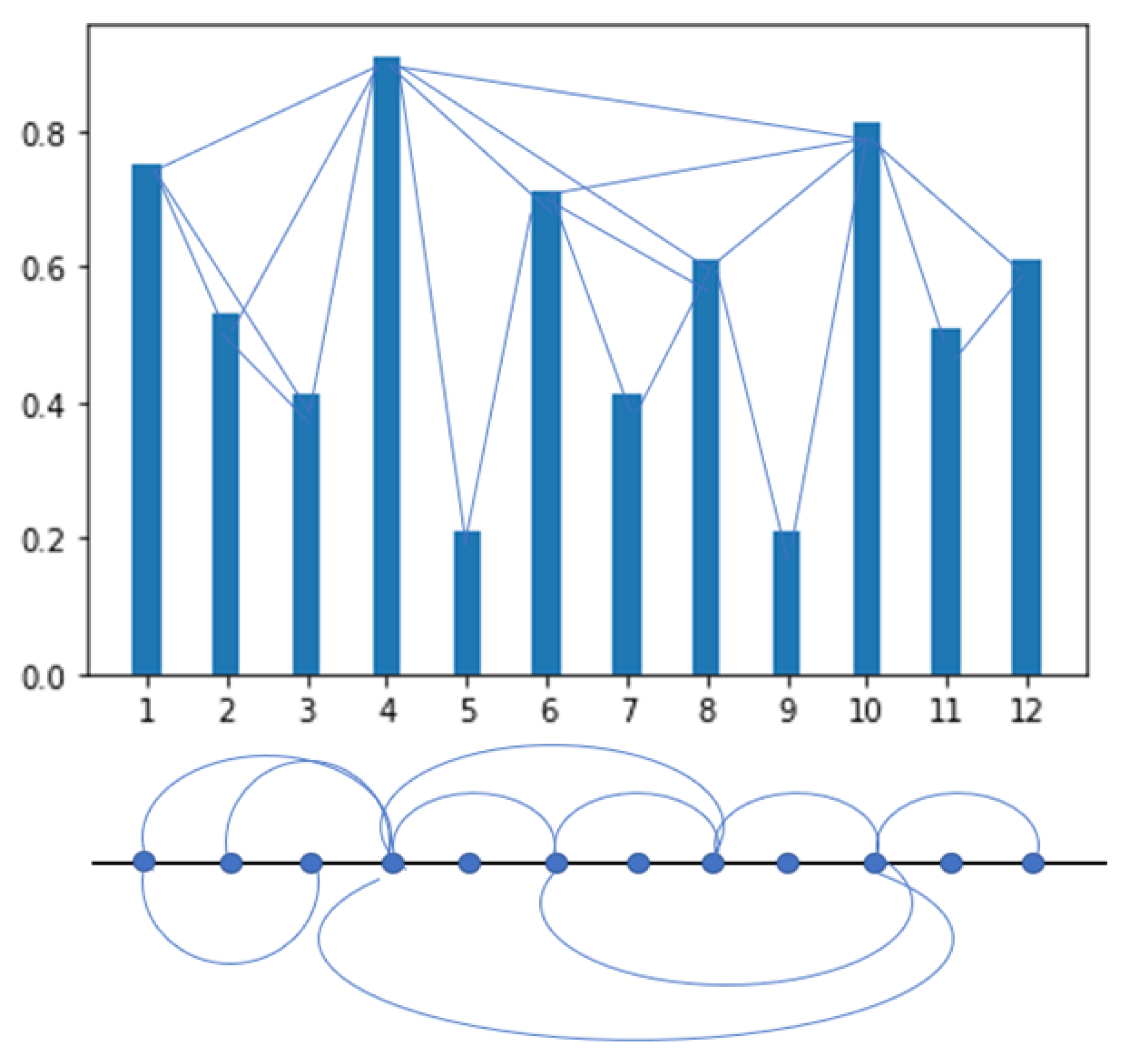[70] using the ts2vg library in Python, with which it is possible to easily transform a time series into a graph with the characteristics associated with the series. Periodic time series will result in regular graphs while random time series will generate random graphs. The method can be formally defined as: two independent data ((da, xa) and (db, xb)) will have visibility between them and therefore in the associated graph their nodes will be connected if other data (dc, xc) located between them meet the following formula:

$$x_c<x_b+\left(x_a-x_b\right)\frac{d_b-d_c}{d_b-d_a}$$

(5)

Figure 5 shows the data of a time series represented in a graph and the connections that are generated by the visibility method, that is, the data that have visibility in the graphical representation and by applying the previous formula by which it is specified in which cases the values will be related. The graph is generated with the edges corresponding to those data related to each other through the visibility method.

From the graph obtained, the correlation matrix to be entered as input in the StellarGraph model in this experiment is calculated, a univariate time series with 10,289 observations is used from which a correlation matrix is generated. Being a univariate series, the resulting correlation is equal to 1 since the relationship of each observation with itself is evaluated. There are no values other than 1 in this result unless there are different variables with which to make the comparison.

In order to better understand the peculiarities of the data used in the training and validation of the time series, a study of it and its characteristics is carried out.

The stationarity of the series is verified using the Dickey Fuller Augmented test (ADF) [71] and the Philips Perrón test (PP) [72], the result of which yields a p-value that allows us to reject the null hypothesis, establishing that there is no stationarity as shown in

Table 1. Time series analysis.

ADF Values	PP Values	Metrics
−1.753	−1.451	Statistical test
0.404	0.558	p-value
10248.000	10,248.000	Number of observations
−2.862	−2.860	Critical value (5%)

.

The graphical representation of the series allows verifying these results, as can be seen in Figure 6.

The data stored in the dataframe are divided into two datasets, one corresponding to the data that are used for model training and contain 80% of the total observations, and the other 20% for testing. The training set is divided, in turn, into two subsets by applying 10% of the total data to the validation of the model, resulting in a division for this set of 70–10% of the total data used in the investigation, which allow measuring the learning of the model and evaluating its performance. In this experiment, the data were normalized to values [0,1].

3.2. Evaluation Metrics

For the evaluation of the performance of the BiLSTM-GCN combined proposal presented in this work, the four most used error metrics were chosen. RMSE and MAPE are metrics used to measure the prediction error and therefore the performance of a neural network. The RMSE represents the root between the differences of the predicted and observed values, while the MAPE is the average of the percentage errors in absolute value. The lower this value, the better the prediction. Frechtling [73] stated that MAPE values between 10% and 20% are considered a good prognosis, and those between 20% and 30% are acceptable, while it is difficult to obtain less than 10% due to the nonlinear nature of the variables.

The value of R2 is closely related to MSE, which is the proportion of the total variance of the variable explained by the regression and is also used to evaluate the performance of the model. It is the amount of variation in the dependent attribute of the output that is predictable from the independent variable(s) of the output. The closer to 1 this value is, the better the performance of the network.

3.3. Model Parameters

With the use of ANNs, it is necessary to determine the values of some parameters to try to improve precision and avoid overfitting. The adjusted hyperparameters for the BiLSTM-GCN combined proposal are the following:

-

Learning rate: A value that is too low may make it necessary to increase the number of epochs and make training slower.

-

Batch size: Determines how many samples will be analyzed before updating the model parameters.

-

Epoch: Determines how many times the entire dataset will be trained.

-

Hidden layers: The complexity of the model is determined by the number of neurons and hidden chaos. This defines the learning capacity of the model. For the selection of the number of hidden layers, different units were experimented with, selecting the optimal value by comparing the evaluation metrics.

-

Optimization algorithm: The choice of the optimization algorithm can have a notable impact on the learning of the models. It updates the parameter values based on the set learning rate. In this case, Adam was selected because it tries to combine the advantages of RMSProp (similar to gradient descent) together with the advantages of gradient descent with momentum [74].

The choice of parameters was made following the recommendations of Goodfellow [75] of making multiple comparisons using a fixed number of cycles, where said number is determined according to computational limitations and if the model reaches overfitting. The values selected for each of these parameters are reflected in

Table 2. Selected parameters for the combined model proposed in this work and the DNN models implemented for comparative purposes.

Model	Learning Rate	Batch	Epoch	Hidden Layers	Neurons	Optimizer
BiLSTM	0.001	25	100	3	50	Adam
GCN-LSTM	0.001	32	50	2/1	16,10/100	Adam
BiLSTM-GCN	0.001	32	50	2	10	Adam

.

For the GCN-LSTM model, the number of layers that correspond to each model and the neurons included in each of the layers are specified separately. The model has two GCN layers with 16 and 10 neurons, respectively, and 1 LSTM layer with 100 neurons.

For the AutoRegresive Integrated Moving Average (ARIMA) (p, d, q) model, the use of the pyramid-arima library (PMDARIMA) was chosen, which allows the analysis of time series through the auto-arima function, which allows finding the optimal order and the optimal seasonal order based on the Akaike Information Criterion (AIC) [76] and the Bayesian Information Criterion (BIC) [77].

The ARIMA model derives from its three components Autoregressive (AR), Integrated (I) and Moving Averages (MA); for the analysis of a time series, it is necessary to find the most appropriate values (p, d, q). The parameter d of the model refers to the number of times that the series has been differentiated to make it stationary. An AR(p) process has the first p terms of the partial autocorrelation function different from zero and the rest are null. Finally, an MA(q) process has the first q terms of the autocorrelation function different from zero and the rest are null. For the present experiment, the parameters used were ARIMA (1, 1, 1).

In order to determine the efficiency of an algorithm, it is necessary to take into account its computational complexity. The most common way is by using the Big-O notation. This notation allows representation of the upper limit of processing of an algorithm. In neural networks, the complexity is determined by the layers that compose it, so the complexity of the network is the sum of the complexity of each of its layers.

The complexity of the three neural network models studied is as follows in

Table 3. Time complexity of DNN models.

Neural Network	Complexity Time
BiLSTM	O(2(4ih + 4h2 + 3 h + ho))
GCN–LSTM	O(LA0i + Lni2) + O(W)
BiLSTM-GCN	O(ih + ho)

.

For the BiLSTM-type network, the complexity is defined by the one determined for duplicate LSTM networks, and this is W = (4dH + 4H2 + 3H + Ho), where i defines the number of inputs, o the number of outputs and h the number of neurons in the hidden layer.

In the BiLSTM-GCN model, the models are pre-trained, so the complexity is defined solely in terms of the dense layers incorporated into the outputs.

L represents the number of layers, A0 the number of non-0 values in the adjacency matrix A, i the number of entries and n the number of nodes in the layer.

In all cases, it is an asymptotic notation in which the computation time increases linearly depending on the data entered, however, a significant difference is evident in the complexity of the new proposed model, whose processing is easier.

3.4. Experimental Results

The performance of the BiLSTM-GCN combined proposal described in this work is compared to the other referenced models: BiLSTM; GCN-LSTM combined model; ARIMA [78], a method that predicts future data by adjusting the time series in a parametric model; and PROPHET, an open source library designed to forecast univariate time series. It is a generalization of an additive regression model, which is broken down into three main components (trend, seasonality and holidays), plus additional regressors.

Table 4. Model Performance in terms of MSE, RMSE, R², MAPE and Time. The best values for each metric are in bold.

	MSE	RMSE	R2	MAPE	Time
ARIMA	81.219	9.012	0.716	22.500	5.23 s
PROPHET	134.050	11.580	0.834	14.380	6.43 s
BiLSTM	16.100	4.012	0.951	7.750	2.57 s
GCN-LSTM	17.829	4.220	0.947	7.630	2.66 s
BiLSTM-GCN	15.610	3.850	0.955	7.410	2.10 s

shows the results obtained for the BiLSTM-GCN combined model and the other referenced models. It can be seen that the BiLSTM-GCN model is the one that obtains the best performance in the predictions under all the evaluation metrics, demonstrating its effectiveness for the forecast of the oil prices of the West Texas Intermediate (WTI) crude oil price index.

In the following figures, the performance of the different models used can be seen graphically based on the results obtained in Table 4. In these graphics, lower RMSE, MSE and MAPE obtained in the new hybrid model are observed, improving the results of the models separately, and a slightly higher R² value, which indicates a more accurate result with test data. Given the results of the ARIMA and PROPHET models, there is a distortion in the graphical representation of the results, by which it has been decided not to show them in Figure 7.

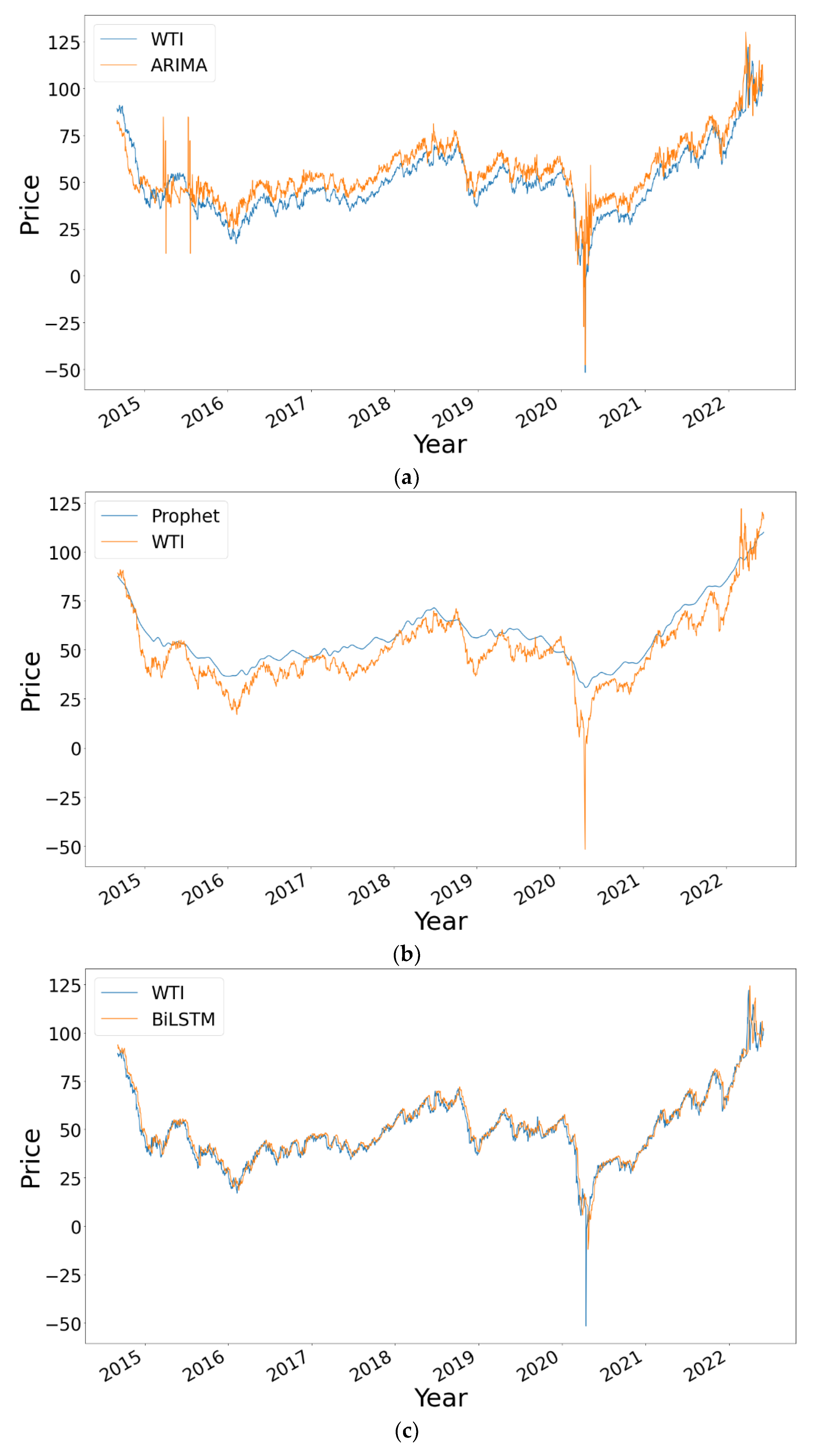
In order to highlight the difference among the results obtained and also for visualization purposes, Figure 8 shows those obtained by the five models from the data relating to the test set, which consists of 20% of the total data from the WTI time series. The closer the prediction line is to the real value, the more accurate the result obtained by the model is and, therefore, the better the predictions it makes. The graphs belonging to the three DNN model-based approaches (BiLSTM, GCN-LSTM and BiLSTM-GCN) show predictions very close to the real values of the price of the WTI index.

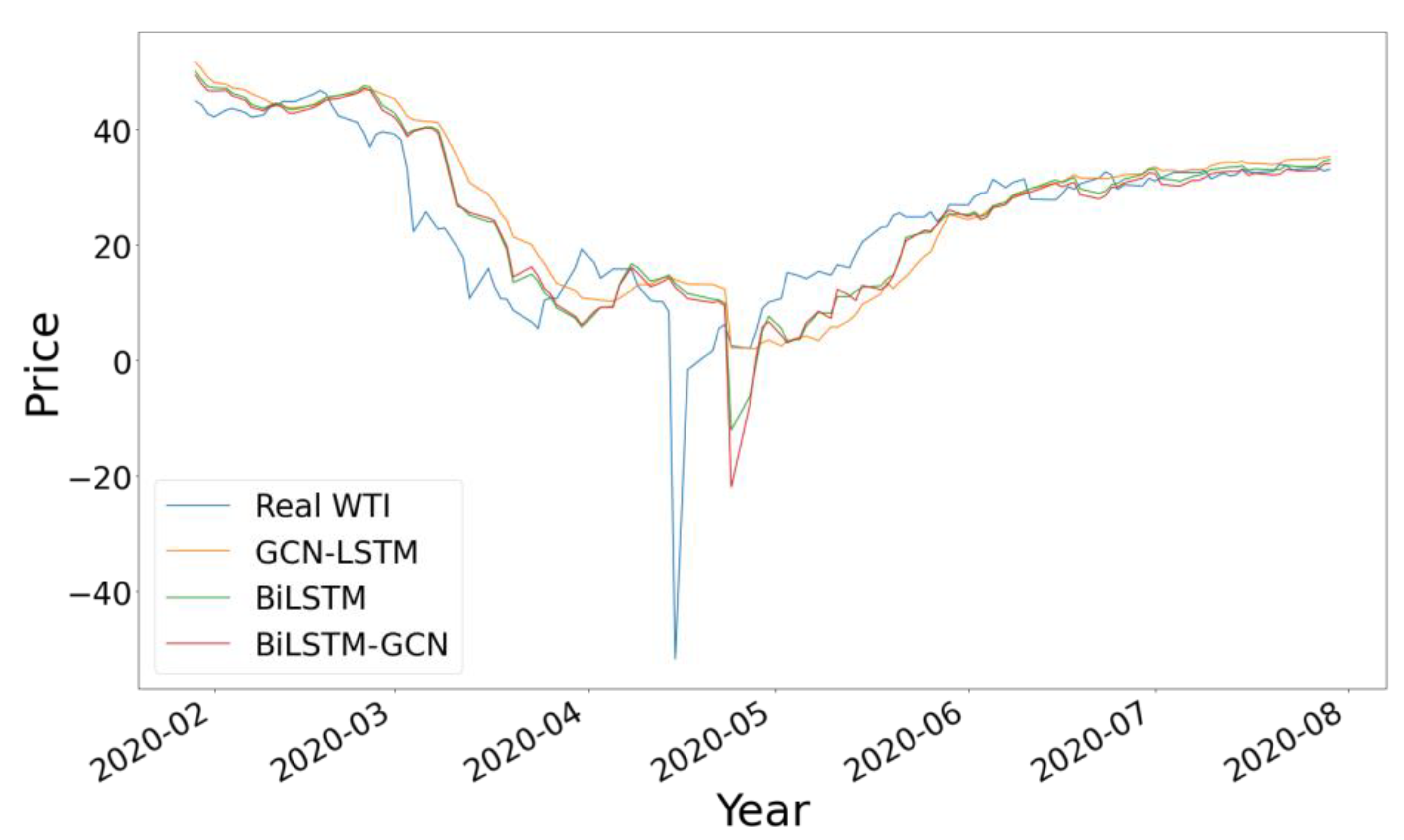
To further highlight the difference between these three results, in Figure 9 we show the comparison with the data corresponding to the year 2020, including only the three neural network models, observing the highest precision in the results of the BiLSTM-GCN model with greater approximation to the true value.

4. Discussion

From the results obtained, it is observed that the models based on LSTM and GCN have better performance and better prediction accuracy than the ARIMA and PROPHET models with a significantly lower error than the latter. For the RMSE metric, our proposal reduces the error by 57.3% compared to the traditional ARIMA statistical technique and 65.5% compared to the PROPHET model, while for DNN models the reduction margin error is 4.07% and 8.7% for BiLSTM and GCN-LSTM, respectively.

These results are mainly due to the fact that methods such as ARIMA and PROPHET have difficulties in the treatment of large, complex and nonstationary time series, even when differentiated to make them stationary. The worst performance of the GCN-LSTM combined model is due to the fact that this type of network considers the spatial characteristics and not the characteristics of the time series. The combination of the BiLSTM and GCN models provides the underlying advantages of both types of DNN, improving the analysis of the series and allowing the error to be minimized. This combined approach also yields better results in execution times, because it implements two pre-trained models and consists of fewer layers and fewer neurons per layer, so data processing through the model is faster.

The BiLSTM-GCN model has the ability to successfully capture the spatial and temporal characteristics of the data related to the price of WTI oil, not being limited to the prediction of this time series, but it is also possible to apply its use to the prediction of time series of various domains. The capture of spatial and temporal features is possible by combining both models. The BiLSTM model allows establishing the temporal relationships between the observations from the data in the form of a time series, while the GCN model is able to establish the spatial relationships through the graph generated from the data, in which the link between nodes is established by means of the visibility method, which allows the convolutional network of graphs to make predictions of the relationships between the nodes, that is, in their spatial characteristic independently of the temporal one.

In order to verify if there is a statistically significant difference, and thereby corroborate the efficiency of the neural network, the Friedman test [79] is performed, through which it can be confirmed if the null hypothesis is rejected, which establishes that the average of each of the predictions made with the different methods is the same as the others (see

Table 5. Friedman test results applied to DNN model predictions.

Statistical Value	280.303
p-Value	1.821 × 10−60

), and that consists of the comparison of the medians of two groups of data. The Friedman test is applied to the results obtained by the neural network models, since these are the most accurate results.

The results of the test including all the models used in the experiment reflect a p-value less than 0.05, so we can reject the null hypothesis, having sufficient evidence to conclude that the means of the predictions made have significant differences.

Given that the result of the Friedman test is significant, we can conclude that at least two of the groups compared are significantly different, but it is not possible to know which ones. Therefore, the Wilcoxon test [80] is applied between each pair of groups with the following results in

Table 6. Wilcoxon test results.

Compared Data	Statistical Value	p-Value
WTI and BiLSMT	19441.0	0.024
WTI and GCN-LSTM	14162.0	9.591 × 10−9
WTI and BiLSTM-GCN	21371.0	0.322

. The results show how the only pair of data that allows us to reject the null hypothesis is the one corresponding to the original data of the WTI series with the predictions obtained by the BiLSTM-GCN model, corroborating a greater precision in the results of this model.

In order to provide a detailed analysis of the model error, a series of statistical tests and visual representations are carried out to confirm the efficiency of the model.

It was decided to calculate the value of F-statistic and its Prob (F-statistic), whose null hypothesis establishes that all the parameters used in the regression are 0 and that it does not help to explain the dependent variable. In this case, it would not find a relationship between the real value of the time series and the prediction. The resulting value is very small, so the null hypothesis is rejected, as shown in

Table 7. Statistical results.

Values	Statistical Value
Kurtosis	47.72
F-Statistic	81.14
Prob (F-Statistic)	1.03 × 10−18

.

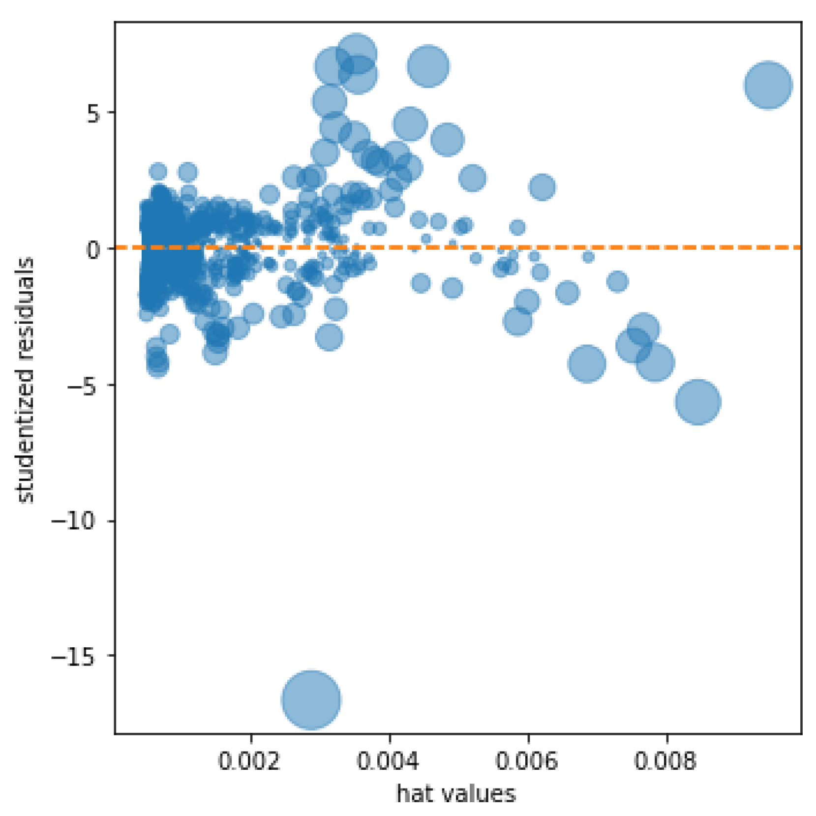
The resulting kurtosis measure measures the higher or lower concentration of the data around the mean; a positive coefficient indicates a higher concentration of the data around the mean, while a negative coefficient reflects a lower concentration. The result of the proposed model reflects a high concentration around the mean; this result is graphically supported by the result of reflecting the influence plot of Figure 10 in which the studentized residuals are shown together with the hat values, of special interest to detect outliers in the predictions. The graph shows a small number of outliers relative to the number of observations studied.

The accumulated error of the 10,289 observations, which consists of the sum of the errors of all the predictions, has a result of 871.31, which gives it at an average error of 0.084 for each observation.

The research reflected in this work indicates the performance demonstrated when combining different types of neural networks, in this case a GCN and RNN, which, due to their different qualities, have been able to capture the relationships between the data of the time series studied and demonstrate a better performance than separate models.

5. Conclusions and Future Lines of Research

This article proposes a novel approach for time series forecasting that unites the performance of BiLSTM and GCN-type networks. A network of graphs is used that, applied to the prediction of a time series, manages to capture its characteristics, converting it into a graphic representation of the data. This network is combined with the potential of BiLSTM-type networks for time series forecasting, obtaining from both outputs a third model that, with the characteristics of the previous two, manages to obtain results that improve the performance of both models separately and traditional statistical techniques such as ARIMA.

Thanks to the results of this research, the ability to combine different types of neural networks [81], conceived for different purposes, for the prediction of economic time series with results that improve the existing literature [82] and those obtained by different traditional forecasting techniques, is clear.

Based on the work carried out in this research and the capacity of the new model to capture the characteristics of the time series to be analyzed, some studies will be carried out on the feasibility of the proposed hybrid model for the prediction of other economic values with different characteristics and its comparison with the models reflected in this document, analyzing the adaptability of the model to time series with different characteristics.