Practical Exponential Stability of Impulsive Stochastic Food Chain System with Time-Varying Delays

Abstract

This paper studies the practical exponential stability of an impulsive stochastic food chain system with time-varying delays (ISOFCSs). By constructing an auxiliary system equivalent to the original system and comparison theorem, the existence of global positive solutions to the suggested system is discussed. Moreover, we investigate the sufficient conditions for the exponential stability and practical exponential stability of the system, which is given by Razumikhin technique and the Lyapunov method. In addition, when Razumikhin’s condition holds, the exponential stability and practical exponential stability of species are independent of time delay. Finally, numerical simulation finds the validity of the method.

1. Introduction

It is important to link community members into a whole group directly or indirectly through food in an ecosystem. This food link is called a food chain because of the important role that food chains play in the ecosystem, and this reflects the universality of natural phenomena. For example, algae, shrimp and fish form a three-group food chain. Recently, there has been much research in the literature regarding the food chain model [1,2,3]. In particular, the classical deterministic food chain model takes the following form:

$$\left\{\begin{array}{c}d{x}_1\left(t\right)=x_1\left(t\right)\left[r_1-a_{11}{x}_1\left(t\right)-a_{12}{x}_2\left(t\right))\right]dt\hfill \\ d{x}_2\left(t\right)=x_2\left(t\right)\left[-r_2+a_{21}{x}_1\left(t\right)-a_{22}{x}_2\left(t\right)-a_{23}{x}_3\left(t\right)\right]dt\hfill \\ d{x}_3\left(t\right)=x_3\left(t\right)\left[-r_3+a_{32}{x}_2\left(t\right)-a_{33}{x}_3\left(t\right)\right]dt\hfill \end{array}\right.$$

(1)

where $x_1\left(t\right)$ denote the densities of prey, $x_2\left(t\right)$ denotes the densities of an intermediate predator and $x_3\left(t\right)$ denotes the densities of top predators in a food chain at time t. $r_1>0$ is the growth rate of prey, $r_2>0$ is the mortality rates of the intermediate predator and $r_3>0$ is the mortality rates of the top predator. $a_{12}$ and $a_{23}$ are capture rates; food conversion rates are expressed as $a_{21}$ and $a_{32}$. $a_{ii}$$(i=1,2,3)$ is the rate of intraspecific competition for the three species. All parameters $a_{ij}$($i,j=1,2,3$) are positive.

It is well known that populations are affected by environmental white noise [4,5]. However, time delays cannot be ignored in biological models, which will lead to system performance degradation and even instability in many practical systems [6,7,8,9,10]. Therefore, the delay problem has received widespread attention, and a large number of results on the stability of stochastic population systems have been published in the literature. On the other hand, due to some natural factors, species are often subject to discrete changes in relatively short time intervals, such as floods, droughts, earthquakes, fires, plagues, etc. Impulse perturbations have been widely studied in ecology, population dynamics and biological systems. Various population dynamical systems have been used in the study of impulsive differential equations [6,11,12,13,14,15,16,17,18,19,20,21,22,23]. Lu [11] found that impulse disturbance plays a vital role in maintaining ecological balance in a random predator–prey model with delay and impulses. Zhao and Wang [23] found that the impulsive effect has an impact on the periodic equilibrium of the stochastic one-predator two-prey model. In recent years, with the development of impulsive stochastic differential equations with delays, many researchers have begun to pay attention to such systems [24,25,26,27,28,29,30,31,32,33,34]. Exponential stability is the most important concept in modern control theory [24]. In many physical systems, such stability is sometimes too strong to be satisfied. However, when the origin is not necessarily an equilibrium point, it is observed that the expected state of a system may be mathematically unstable, but the system can oscillate sufficiently within a small neighborhood of the state. Performance in this situation is considered to be acceptable, but discussion is still very important. This case gives rise to the concept of practical stability. A number of interesting results have been reported regarding the practical stability of different systems [35,36,37]. However, as far as we know, no papers on the practical exponential stability of the impulsive stochastic three food chain systems with time-varying delays have been published so far. This situation motivates the research of this paper.

Following the discussion above, we will investigate the exponential stability and practical exponential stability of the impulsive stochastic food chain system. The impulsive stochastic food chain system with time-varying delays is presented in the following form:

$$\left\{\begin{array}{c}d{x}_1\left(t\right)=x_1\left(t\right)\left[r_1-a_{11}{x}_1(t-{\tau }_{11}\left(t\right))-a_{12}{x}_2(t-{\tau }_{12}\left(t\right)))\right]dt\hfill \\ +{\sigma }_1{x}_1\left(t\right)d{B}_1\left(t\right),\hfill \\ d{x}_2\left(t\right)=x_2\left(t\right)\left[r_2+a_{21}{x}_1(t-{\tau }_{21}\left(t\right))-a_{22}{x}_2\left(t\right)-a_{23}{x}_3(t-{\tau }_{23}\left(t\right))\right]dt\hfill \\ +{\sigma }_2{x}_2\left(t\right)d{B}_2\left(t\right),\hfill \\ d{x}_3\left(t\right)=x_3\left(t\right)\left[-r_3+a_{32}{x}_2(t-{\tau }_{32}\left(t\right))-a_{33}{x}_3(t-{\tau }_{33}\left(t\right))\right]dt\hfill \\ +{\sigma }_3{x}_3\left(t\right)d{B}_3\left(t\right),\hfill \\ x_i\left(t_k^{+}\right)=(1+{\alpha }_{ik})x_i\left(t_k\right),x_i\left(t_k^{-}\right)=x_i\left(t_k\right),kϵN,\hfill \\ x_i\left(\theta \right)={\varphi }_i\left(\theta \right),-{\tau }_0\le \theta \le 0,t\ge 0,0\le {\tau }_i\left(t\right)\le {\tau }_0,i=1,2,3,\hfill \end{array}\right.$$

(2)

where ${\sigma }_i(i=1,2,3)$ are the coefficients of the effects of environmental stochastic perturbations on prey, intermediate predators and top predators, respectively. ${\tau }_{ij}\left(t\right)>0$ represents the time-varying delay and $\mathbf{\varphi }\left(\theta \right)={({\varphi }_1\left(\theta \right),{\varphi }_2\left(\theta \right),{\varphi }_3\left(\theta \right))}^T\in U$, and $U=C([-{\tau }_0,0],R_{+}^3)$ represent the space of all the continued functions. Throughout the year, the sun, the stars and the moon, the producers and the consumers of the world’s resources, and the predators and prey work in harmony to form the natural system of the Earth. Therefore, by adjusting system parameters and noise intensity to study the actual exponential stability law of the food chain, we can better understand and follow the natural law.

The remainder of this paper is organized as follows. In Section 2, some definitions, notations and lemmas are given. In Section 3, the existence of global positive solutions for Model (2) is discussed. In Section 4, using the Razumikhin technique and the Lyapunov method, the practical exponential stability and exponential stability of Model (2) are investigated. If the Razumikhin condition holds, the practical exponential stability and exponential stability of the species are independent of time delays. In Section 5, simulation results verify the correctness of the theoretical conclusions. The conclusion of this paper contains some general comments.

2. Prilimary

The Brownian motions $B_i\left(t\right)(i=1,2,3)$ are defined on a complete probability space $(\mathsf{\Omega },{\mathcal{F}}_t,{\left({\mathcal{F}}_t\right)}_{t\ge 0},\mathbb{P})$ with a filtration ${\left({\mathcal{F}}_t\right)}_{t\ge 0}$. The filtration ${\left({\mathcal{F}}_t\right)}_{t\ge 0}$ is right continuous, increasing and contains all $\mathbb{P}$-null sets. Further, $0<t_1<t_2<\cdots <t_k<\cdots$ and ${lim}_{k\to +\infty }{t}_k=+\infty$. Biologically speaking, we only care about the positive solution to the equation. For convenience, we will use $A_{ij}=A_i(t-{\tau }_{ij}\left(t\right))y_i(t-{\tau }_{ij}\left(t\right)),i,j=1,2,3$. Let $A_i\left(t\right)={\left({\prod }_{j=1}^k(1+{\alpha }_{ij})\right)}^{-t}{\prod }_{t_k<t}(1+{\alpha }_{ik})$, $x_i\left(t\right)=A_i\left(t\right)y_i\left(t\right)$, i = 1, 2, 3, $t\ge 0$. $J_1=r_1+{\sum }_{j=1}^{k}ln(1+{\alpha }_{1j})-0.5{\sigma }_1^2$, $J_i=-r_i+{\sum }_{j=i}^{k}ln(1+{\alpha }_{ij})-0.5{\sigma }_i^2,i=2,3$.

Definition 1. 

Let $\mathit{x}\left(t\right)={(x_1\left(t\right),x_2\left(t\right),x_3\left(t\right))}^T$ be a solution to Model (2).

1. 

For $p>0$, the Model (2) is said to be pth moment practical exponential stability. If there exist positive constants $D_1>0$, $D_2\ge 0$ and $\lambda >0$ such that

$${E\left|\mathit{x}\left(t\right)\right|}^p\le D_{1}E{\left|\mathbf{\varphi }\right|}_C^p{e}^{-\lambda (t-t_0)}+D_2,t\ge t_0.$$

(3)

In particular, when $D_2=0$, Model (2) is said to be the pth moment exponential stability.

2. 

If $p>0$ and ${lim}_{t\to +\infty }E{\left|\mathit{x}\left(t\right)\right|}^p=0$, a.s., then Model (2) is said to be pth moment extinction.

3. 

If $p>0$ and ${lim}_{t\to +\infty }E{\left|\mathit{x}\left(t\right)\right|}^p>0$, a.s., then Model (2) is said to be pth moment persistence.

For Model (2), we always assume $\left(T\right)$∃$M_i>0$, $N_i>0$ such that ∀$k\in N$, ${\prod }_{j=1}^k(1+{\alpha }_{ij})\le M_i$, ${\sum }_{j=1}^k(1+{\alpha }_{ij})\le N_i,i=1,2,3$.

Lemma 1. 

The solution $x\left(t\right)$ of the predator–prey Model (2) obeys

$$\underset{t\to +\infty }{lim\; sup}\frac{ln{x}_i\left(t\right)}{lnt}\le 1+\underset{t\to +\infty }{lim\; sup}\frac{{\sum }_{0<t_k<t}ln(1+{\alpha }_{ik})}{lnt}a.s.,1\le i\le 3,t>0.$$

(4)

Proof. 

The proof method of Lemma 1 is similar to that in [4], so it is omitted. □

3. Global Positive Solutions

Consider the following auxiliary model:

$$\left\{\begin{array}{c}{\displaystyle d{y}_1\left(t\right)=y_1\left(t\right)[r_1+\sum _{j=1}^{k}ln(1+{\alpha }_{1j})-a_{11}{A}_{11}}\hfill \\ -a_{12}{A}_{12}]dt+{\sigma }_1{y}_1\left(t\right)d{B}_1\left(t\right),\hfill \\ {\displaystyle d{y}_2\left(t\right)=y_2\left(t\right)[-r_2+\sum _{j=1}^{k}ln(1+{\alpha }_{2j})+a_{21}{A}_{21}}\hfill \\ -a_{22}{A}_{22}-a_{23}{A}_{23}]dt+{\sigma }_2{y}_2\left(t\right)d{B}_2\left(t\right),\hfill \\ {\displaystyle d{y}_3\left(t\right)=y_3\left(t\right)[-r_3+\sum _{j=1}^{k}ln(1+{\alpha }_{3j})+a_{32}{A}_{32}}\hfill \\ -a_{33}{A}_{33}]dt+{\sigma }_3{y}_3\left(t\right)d{B}_3\left(t\right),\hfill \\ y_i\left(0\right)={\varphi }_i\left(0\right),y_i\left(\theta \right)={\varphi }_i\left(\theta \right),i=1,2,3,-{\tau }_0\le \theta \le 0,t\ge 0.\hfill \end{array}\right.$$

(5)

Theorem 1. 

Under the condition that the comparison theorem is established in [6], in Model (5), for any given initial condition $\mathbf{\varphi }\left(\theta \right)={({\varphi }_1\left(\theta \right),{\varphi }_2\left(\theta \right),{\varphi }_3\left(\theta \right))}^T$, ${\varphi }_i\left(\theta \right)\in C([-{\tau }_0,0],{\mathbb{R}}^{+})$$(i=1,2,3)$, there is a unique solution $y\left(t\right)$ on $t\in {\mathbb{R}}^{+}=[0,\infty )$, with $y\left(\theta \right)=\varphi \left(\theta \right)$, $\theta \in [-{\tau }_0,0)$, and the solution will remain in ${\mathbb{R}}_{+}^3$ with Probability 1.

Proof. 

Make the substitution $u_i=ln{y}_i$; then, using Itô’s formula, we can rewrite the system (3.2) as follows:

$$\left\{\begin{array}{c}{\displaystyle d{u}_1\left(t\right)=y_1\left(t\right)[J_1-a_{11}{A}_{11}{e}^{u_1(t-{\tau }_{11}\left(t\right))}}\hfill \\ -a_{12}{A}_{12}{e}^{u_2(t-{\tau }_{12}\left(t\right))}]dt+{\sigma }_{1}d{B}_1\left(t\right),\hfill \\ {\displaystyle d{u}_2\left(t\right)=y_2\left(t\right)[J_2+a_{21}{A}_{21}{e}^{u_1(t-{\tau }_{21}\left(t\right))}}\hfill \\ -a_{22}{A}_{22}{e}^{u_2(t-{\tau }_{22}\left(t\right))}-a_{23}{A}_{23}{e}^{u_3(t-{\tau }_{23}\left(t\right))}]dt+{\sigma }_{2}d{B}_2\left(t\right),\hfill \\ {\displaystyle d{u}_3\left(t\right)=y_3\left(t\right)[J_3+a_{32}{A}_{32}{e}^{u_1(t-{\tau }_{32}\left(t\right))}}\hfill \\ -a_{33}{A}_{33}{e}^{u_3(t-{\tau }_{33}\left(t\right))}]dt+{\sigma }_{3}d{B}_3\left(t\right),\hfill \end{array}\right.$$

(6)

where $u_i\left(0\right)={\varphi }_i\left(0\right),u_i\left(\theta \right)={\varphi }_i\left(\theta \right),i=1,2,3,-{\tau }_0\le \theta \le 0,t\ge 0$. $J_1=r_1+{\sum }_{j=1}^{k}ln(1+{\alpha }_{1j})-\frac{1}{2}{\sigma }_1^2$, $J_i=r_2+{\sum }_{j=1}^{k}ln(1+{\alpha }_{2j})-\frac{1}{2}{\sigma }_2^2,i=1,2$. Applying the comparison theorem 2.1 in [38], we obtain $y_i\le u_i\left(t\right)a.s.i=1,2,3$ for $t\in (0,{\tau }_e)$, According to Theorem 2.1 in [5], Model (6) has a global solution $u\left(t\right)={(u_1\left(t\right),u_2\left(t\right),u_3\left(t\right))}^T$, and then we have ${\tau }_e=+\infty$, for which the proof is similar to [39]. □

Theorem 2. 

If $\mathit{y}\left(t\right)={(y_1\left(t\right),y_2\left(t\right),y_3\left(t\right))}^T$ is a solution to (5), then $\mathit{x}\left(t\right)=(x_1\left(t\right),x_2\left(t\right),$ and $x_3{\left(t\right))}^T={(A_1\left(t\right)y_1\left(t\right),A_2\left(t\right)y_2\left(t\right),A_3\left(t\right)y_3\left(t\right))}^T$ is a solution to (2).

Proof. 

Assume $\mathit{y}\left(t\right)={(y_1\left(t\right),y_2\left(t\right),y_3\left(t\right))}^T$ is a solution to (5),

(i)

When $t\ge 0,t\ne t_k$, we have

$$\begin{array}{cc}\hfill A_i\left(t\right)& ={\left(\prod _{j=1}^k(1+{\alpha }_{ij})\right)}^{-t}\prod _{t_l<t}(1+{\alpha }_{il}),i=1,2,3.\hfill \end{array}$$

Thus,

$$\begin{array}{cc}\hfill ln{A}_i\left(t\right)& =-t\sum _{j=1}^{k}ln(1+{\alpha }_{ij})+ln\prod _{t_l<t}(1+{\alpha }_{il}),\hfill \end{array}$$

Take the derivative of both sides:

$$\begin{array}{cc}\hfill d{A}_i\left(t\right)& =-\sum _{j=1}^{k}ln(1+{\alpha }_{ij})A_i\left(t\right)dt.\hfill \end{array}$$

Then,

$$\begin{array}{ccc}\hfill d{x}_1\left(t\right)& =& d\left[A_1\left(t\right)y_1\left(t\right)\right]\hfill \\ & =& {\displaystyle A_1\left(t\right)y_1\left(t\right)[r_1+\sum _{j=1}^{k}ln(1+{\alpha }_{1j})-a_{11}{A}_{11}-a_{12}{A}_{12}]dt}\hfill \\ & -& \sum _{j=1}^{k}ln(1+{\alpha }_{1j})A_1\left(t\right)y_1\left(t\right)dt+{\sigma }_1{A}_1\left(t\right)y_1\left(t\right)d{B}_1\left(t\right)\hfill \\ & =& x_1\left(t\right)\left[r_1-a_{11}{x}_1(t-{\tau }_{11}\left(t\right))-a_{12}{x}_2(t-{\tau }_{12}\left(t\right))\right]dt\hfill \\ & +& {\sigma }_1{x}_1\left(t\right)d{B}_1\left(t\right).\hfill \end{array}$$

(7)

Similarly, we can obtain a stochastic equation for $x_2$ and $x_3$ in the form of (1.2) with the initial values and $x_i\left(0\right)={\left[{\prod }_{j=1}^k(1+{\alpha }_{ij})\right]}^{-0}{\prod }_{t_l<0}(1+{\alpha }_{il})y_i\left(0\right)=y_i\left(0\right)={\varphi }_i\left(0\right)(i=1,2,3)$.

(ii)

When $t=t_k$, we have

$$\begin{array}{cc}\hfill x_i\left(t_k^{+}\right)& =\underset{t\to t_k^{+}}{lim}{A}_i\left(t\right)y_i\left(t\right)=\underset{t\to t_k^{+}}{lim}{\left(\prod _{j=1}^k(1+{\alpha }_{ij})\right)}^{-t}\prod _{t_l<t}(1+{\alpha }_{il})y_i\left(t\right)\hfill \\ \hfill & =(1+{\alpha }_{ik})\prod _{j=1}^k{(1+{\alpha }_{ij})}^{-t_k}\prod _{t_l<t_k}(1+{\alpha }_{il})y_i\left(t_k\right)\hfill \\ \hfill & =(1+{\alpha }_{ik})x_i\left(t_k\right)(i=1,2,3).\hfill \end{array}$$

In addition,

$$\begin{array}{cc}\hfill x_i\left(t_k^{-}\right)& =\underset{t\to t_k^{-}}{lim}{A}_i\left(t\right)y_i\left(t\right)=A_i\left(t_k\right)y_i\left(t_k^{-}\right)=x_i\left(t_k\right).\hfill \end{array}$$

Through proof (i) and (ii) above, we find that $x\left(t\right)={(A_1\left(t\right)y_1\left(t\right),A_2\left(t\right)y_2\left(t\right),A_3\left(t\right)y_3\left(t\right))}^T$ is a solution to (2). □

Remark 1. 

Theorem 2 states that Model (2) also has a unique global positive solution. Model (2) has the same asymptotic behavior as Model (5). That is to say, system (1.2) and (3.1) are equivalent.

4. Practical Exponential Stability

Consider the following stochastic functional differential equations:

$$\left\{\begin{array}{c}d\mathit{x}\left(t\right)=\mathit{f}(t,{\mathit{x}}_t)d\mathit{B}\left(t\right)+\mathit{g}(t,{\mathit{x}}_t)dt,\hfill \\ x\left(t_0\right)=\varphi \left(0\right),x(t_0+\theta )=\varphi \left(\theta \right),{\mathit{x}}_t=\mathit{x}(t+\theta ),-{\tau }_0\le \theta \le 0,t\ge t_0,\hfill \end{array}\right.$$

(8)

where $\mathbf{\varphi }\in C([-{\tau }_0,0],{\mathbb{R}}^n)$, $\mathit{x}\in {\mathbb{R}}^n$, $x_t\in L_{F_t}^p([-{\tau }_0,0],{\mathbb{R}}^n)$, $\mathit{x}:L_{F_t}^p({\mathbb{R}}_{+}\times ([-{\tau }_0,0],{\mathbb{R}}^n))\to {\mathbb{R}}^n$, $\mathit{f}:L_{F_t}^p({\mathbb{R}}_{+}\times ([-{\tau }_0,0],{\mathbb{R}}^n))\to {\mathbb{R}}^{n\times m}$.

The operator is

$$\begin{array}{c}\hfill LV=\left[\frac{\partial V}{\partial t}+{\nabla }_{x}V·f+\frac{1}{2}tr\left(G{G}^T{V}_{xx}\right)\right](t,X).\end{array}$$

Lemma 2. 

Suppose there is a function $V\in C^{1,2}$$([t_0-{\tau }_0,\infty )\times {\mathbb{R}}^n;{\mathbb{R}}_{+})$ and constants $l_1>0$, $\xi >0$, ${\xi }_1>0$, ${\xi }_2>0$, ${\xi }_3\ge 0$, $\eta >0$, $\zeta \ge 0$, $\mu \ge 0$ and $\nu >0$ such that

$$\begin{array}{c}\hfill {\xi }_1{\left|\mathit{x}\right|}^{l_1}\le V(t,\mathit{x})\le {\xi }_2{\left|\mathit{x}\right|}^{l_1}+{\xi }_3,for(t,\mathit{x})\in [t_0-{\tau }_0,\infty )\times {\mathbb{R}}^n.\end{array}$$

(9)

$$\begin{array}{c}\hfill ELV(t,\mathbf{\varphi })\le \xi EV(t,\varphi \left(0\right))+\mu ,fort\ge t_0,\varphi \in C([-{\tau }_0,0],{\mathbb{R}}^n).\end{array}$$

(10)

$$\begin{array}{c}\hfill EV(t+\theta ,\mathbf{\varphi })\le l_{2}EV(t,\varphi \left(0\right))+\zeta ,fort\ge t_0,\theta \in [-{\tau }_0,0],l_2\ge \nu e^{\eta {\tau }_0}.\end{array}$$

(11)

Then,

$$\begin{array}{c}\hfill {E\left|\mathit{x}\left(t\right)\right|}^p\le \frac{{\xi }_2\nu e^{\eta {\tau }_0}}{{\xi }_1}E{\left|\mathbf{\varphi }\right|}_C^p{e}^{-\eta (t-t_0)}+\frac{\nu }{{\xi }_1},t\ge t_0.\end{array}$$

(12)

The system (8) is also considered to have practical exponential stability of pth (see, [37]). In fact, neglecting the impulsive perturbations in Theorem 3.1 [37], the theorem degenerates to Lemma 2.

Remark 2. 

When parameter $\xi >0$, the practical exponential stability of the system (8) depends on parameters $l_1$, ${\xi }_1$, ${\xi }_2$, $l_2$, ν, η and delay constant ${\tau }_0$. It is not concerning the parameters ${\xi }_3\ge 0$, $\mu \ge 0$ and $\zeta \ge 0$. The pth moment practical exponential stability means the pth moment persistence for ecosystems.

Lemma 3. 

Assume that there exists a function $V\in C^{1,2}$$([t_0-{\tau }_0,\infty )\times {\mathbb{R}}^n;{\mathbb{R}}_{+})$ and constants $l_1>0$, $\xi >0$, ${\xi }_1>0$, ${\xi }_2>0$, ${\xi }_3\ge 0$, $\zeta \ge 0$ and $l_2>1$ such that

$$\begin{array}{c}\hfill {\xi }_1{\left|\mathbf{\varphi }\right|}^{l_1}\le V(t,\mathbf{\varphi })\le {\xi }_2{\left|\mathbf{\varphi }\right|}^{l_1}+{\xi }_3,for(t,\mathbf{\varphi })\in [t_0-{\tau }_0,\infty )\times {\mathbb{R}}^n.\end{array}$$

(13)

$$\begin{array}{c}\hfill ELV(t,\mathbf{\varphi })\le -\xi EV(t,\varphi \left(0\right)),fort\ge t_0,\varphi \in C([-{\tau }_0,0],{\mathbb{R}}^n).\end{array}$$

(14)

$$\begin{array}{c}\hfill EV(t+\theta ,\mathbf{\varphi })\le l_{2}EV(t,\varphi \left(0\right))+\zeta ,fort\ge t_0,\theta \in [-{\tau }_0,0].\end{array}$$

(15)

Then,

$$\begin{array}{c}\hfill {E\left|\mathit{x}\left(t\right)\right|}^{l_1}\le \frac{{\xi }_2}{{\xi }_1}E{\left|\mathbf{\varphi }\right|}_C^{l_1}{e}^{-\eta (t-t_0)},\end{array}$$

(16)

where $\eta =min[\xi ,\frac{ln{l}_2}{{\tau }_0}]$.

The system (8) is also said to be the pth moment exponential stability (see [22,37]).

Proof. 

There is the same proof method in [25,37], which is omitted. □

In fact, the pth moment exponential stability means the pth moment extinction for ecosystems.

Theorem 3. 

Let $R_1=r_1+{\sum }_{j=1}^{k}ln(1+{\alpha }_{1j})$, $R_i=-r_i+{\sum }_{j=1}^{k}ln(1+{\alpha }_{ij})(i=2,3)$, and $D=R_1+R_2+R_3+\frac{1}{2}({\sigma }_1^2+{\sigma }_2^2+{\sigma }_3^2)-\frac{{(R_1+a_{21}{A}_1)}^2}{2a_{21}{A}_1}-\frac{{(R_2+a_{32}{A}_2)}^2}{a_{21}{A}_1+a_{32}{A}_2}-\frac{R_3^2}{2a_{32}{A}_2}$. Assume that $A_i<0,i=1,2$, $a_{21}{A}_1+a_{32}{A}_2<0$ and $A_{ij}(t-{\tau }_{ij}\left(t\right))<A_{ij}\left(t\right)(i,j=1,2)$ and the Razumikhin conditions hold:

$$\begin{array}{c}\hfill y_{ij}(t-{\tau }_{ij}\left(t\right))<y_{ij}\left(t\right),t\ge 0(i,j=1,2,3).\end{array}$$

(17)

(1) When $D>0$, the system (5) is the 1stmoment practical exponential stability; that is, the system (2) is also the 1st moment persistence.

(2) When $D<0$, the system (5) is the 1st moment exponential stability; that is, the system (2) is also 1st moment extinction.

Proof. 

Let $\mathit{y}={(y_1,y_2,y_3)}^T$$\in {\mathbb{R}}_{+}^3$ and $\left|\mathit{y}\right|={\sum }_{i=1}^3{y}_i$. Define $V_i\left(y\right)=y_i+ln(y_i+1)(i=1,2,3)$, $V\left(y\right)={\sum }_{i=1}^3{V}_i\left(y\right)$.

Then,

$$\begin{array}{c}\hfill y_i\le V_i\left(\mathit{y}\right)\le 2y_i+1(i=1,2,3),for(t,\mathit{y})\in [-{\tau }_0,\infty )\times {\mathbb{R}}^3.\end{array}$$

(18)

So,

$$\begin{array}{c}\hfill \left|\mathit{y}\right|\le V\left(\mathit{y}\right)\le 2\left|\mathit{y}\right|+3,for(t,\mathit{y})\in [-{\tau }_0,\infty )\times {\mathbb{R}}^3.\end{array}$$

(19)

From the Razumikhin condition (17) and (19), we have

$$\begin{array}{cc}\hfill & EV\left(\varphi \right(\theta \left)\right)\le 2E\left|\varphi \right(\theta \left)\right|+3<2E\left|\varphi \right(0\left)\right|+3\le 2V\left(\varphi \right(0\left)\right)+3.\end{array}$$

(20)

From the Razumikhin condition (17), $a_{ij}>0(1\le i,j\le 3)$, $A_i(t-{\tau }_i\left(t\right))<A_i\left(t\right)(i=1,2)$ and $y_i\left(t\right)\ge 0(i=1,2,3)$, we have

$$\begin{array}{ccc}\hfill L{V}_1& =& (1+\frac{1}{y_1+1})y_1(r_1+\sum _{j=1}^{k}ln(1+{\alpha }_{1j}))-a_{11}{A}_{11}\hfill \\ & -& a_{12}{A}_{12}-\frac{1}{2}\frac{y_1^2}{{(1+y_1)}^2}{\sigma }_1^2\hfill \\ & <& (y_1+1)(r_1+\sum _{j=1}^{k}ln(1+{\alpha }_{1j}))+\frac{1}{2}{\sigma }_1^2\hfill \\ & =& R_1{y}_1^2+R_1+\frac{1}{2}{\sigma }_1^2.\hfill \end{array}$$

(21)

Similarly,

$$\begin{array}{ccc}\hfill L{V}_2& =& (1+\frac{1}{y_2+1})y_2(R_2+a_{21}{A}_{11}-a_{22}{A}_{22}-a_{23}{A}_{23})-\frac{1}{2}\frac{y_2^2}{{(1+y_2)}^2}{\sigma }_1^2\hfill \\ & <& a_{21}{A}_1{y}_1+R_2{y}_2+a_{21}{A}_1{y}_1{y}_2+R_2+\frac{1}{2}{\sigma }_2^2.\hfill \end{array}$$

(22)

$$\begin{array}{c}\hfill L{V}_3<R_3{y}_3+a_{32}{A}_2{y}_2{y}_3+a_{32}{A}_2{y}_2+R_3+\frac{1}{2}{\sigma }_3^2.\end{array}$$

(23)

$$\begin{array}{ccc}\hfill LV& =& L{V}_1+L{V}_2+L{V}_3\hfill \\ & =& R_1{y}_1^2+R_1+a_{21}{A}_1{y}_1+R_2{y}_2+a_{21}{A}_1{y}_1{y}_2\hfill \\ & +& R_3{y}_3+a_{32}{A}_2{y}_2{y}_3+a_{32}{A}_2{y}_2+R_1+R_2+R_3+\frac{1}{2}({\sigma }_1^2+{\sigma }_2^2+{\sigma }_3^2)\hfill \\ & =& (R_1+a_{21}{A}_1)y_1+(R_2+a_{32}{A}_2)y_2+R_3{y}_3+a_{21}{A}_1{y}_1{y}_2\hfill \\ & +& a_{32}{A}_2{y}_2{y}_3+R_1+R_2+R_3+\frac{1}{2}({\sigma }_1^2+{\sigma }_2^2+{\sigma }_3^2)\hfill \\ & \le & \frac{1}{2}{a}_{21}{A}_1{y}_1^2+(R_1+a_{21}{A}_1)y_1+\frac{1}{2}(a_{21}{A}_1+a_{32}{A}_2)y_2^2\hfill \\ & +& (R_2+a_{32}{A}_2)y_2+\frac{1}{2}{a}_{32}{A}_2{y}_3^2+R_3{y}_3+R_1+R_2+R_3+\frac{1}{2}({\sigma }_1^2+{\sigma }_2^2+{\sigma }_3^2)\hfill \\ & \le & \frac{1}{2}{a}_{21}{A}_1{\left(y_1+\frac{R_1+a_{21}{A}_1}{a_{21}{A}_1}\right)}^2-\frac{{(R_1+a_{21}{A}_1)}^2}{2a_{21}{A}_1}\hfill \\ & +& \frac{1}{2}(a_{21}{A}_1+a_{32}{A}_2){\left(y_2+\frac{R_2+a_{32}{a}_2}{a_{21}{A}_1+a_{32}{A}_2}\right)}^2-\frac{{(R_2+a_{32}{A}_2)}^2}{a_{21}{A}_1+a_{32}{A}_2}\hfill \\ & +& \frac{1}{2}{a}_{32}{A}_2{\left(y_3+\frac{R_3}{a_{32}{A}_2}\right)}^2-\frac{R_3^2}{2a_{32}{A}_2}+R_1+R_2+R_3+\frac{1}{2}({\sigma }_1^2+{\sigma }_2^2+{\sigma }_3^2)\hfill \\ & <& R_1+R_2+R_3+\frac{1}{2}({\sigma }_1^2+{\sigma }_2^2+{\sigma }_3^2)\hfill \\ & -& \frac{{(R_1+a_{21}{A}_1)}^2}{2a_{21}{A}_1}-\frac{{(R_2+a_{32}{A}_2)}^2}{a_{21}{A}_1+a_{32}{A}_2}-\frac{R_3^2}{2a_{32}{A}_2}=D\hfill \end{array}$$

(24)

Case (I). When $D>0$, let $D=\xi EV\left(\varphi \right(0\left)\right)$. Then, $ELV\left(\varphi \right(\theta \left)\right)<\xi EV\left(\varphi \right(0\left)\right)$. From Lemma 2, we have

$$\begin{array}{cc}\hfill & E\left|\mathit{x}\left(t\right)\right|\le 2\nu e^{\eta {\tau }_0}E{\left|\mathbf{\varphi }\right|}_C{e}^{-\eta t}+\nu ,t\ge 0,\end{array}$$

(25)

where $2\ge \nu e^{\eta {\tau }_0}$. So, the system (5) is the 1st moment practical exponential stability. That is to say, the system (2) is also 1st moment persistence.

Case (II). When $D<0$, let $\left|D\right|=cEV\left(\varphi \right(0\left)\right)$. Then, $ELV\left(\varphi \right(\theta \left)\right)<-cEV\left(\varphi \right(0\left)\right)$. From Lemma 3, we have

$$\begin{array}{cc}\hfill & E\left|\mathit{x}\left(t\right)\right|\le {2E\left|\mathbf{\varphi }\right|}_C{e}^{-\eta t},t\ge 0,\end{array}$$

(26)

where $\lambda =min[\xi ,\frac{ln2}{{\tau }_0}]$. So, the system (5) is 1st moment exponential stability. In other words, the system (2) is also 1st moment extinction. □

Corollary 1. 

In addition to assumptions T and (4.18), Model (2) also satisfies the following conditions

$$R_1=-a_{21}{A}_1,$$

(27)

$$R_2=-a_{32}{A}_2,$$

(28)

$$R_3=0,$$

(29)

Then,

(I) 

If

$$\begin{array}{cc}\hfill R_1& +R_2+R_3+0.5({\sigma }_1^2+{\sigma }_2^2+{\sigma }_3^2)>0,\hfill \end{array}$$

(30)

the system (2) is 1st practical exponential stability.

(II) 

If

$$\begin{array}{cc}\hfill R_1& +R_2+R_3+0.5({\sigma }_1^2+{\sigma }_2^2+{\sigma }_3^2)<0,\hfill \end{array}$$

(31)

the system (2) is 1st exponential stability.

Proof. 

If the conditions (27)–(29) hold, from (4.17), we have

$$\begin{array}{cc}\hfill LV& \le L{V}_1+L{V}_2+L{V}_3<R_1+R_2+R_3+\frac{1}{2}({\sigma }_1^2+{\sigma }_2^2+{\sigma }_3^2)=D.\hfill \end{array}$$

(32)

From Theorem 3, Corollary 1 is true. □

Remark 3. 

Since the Model (2) contains time delay, it is a non-Markov process. From Theorem 3, we find that under Razumikin condition (17), the persistence criterion (18) and extinction criterion (19) of the species in the Model (2) are independent of time delay. This shows that a non-Markov process can produce Markov effect under certain conditions.

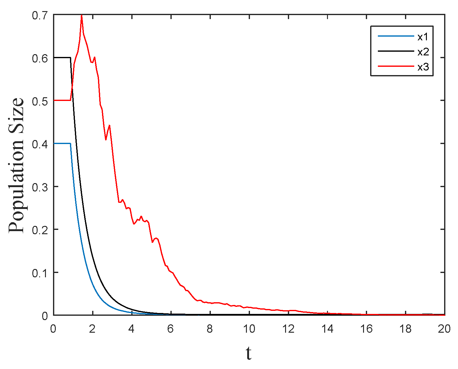
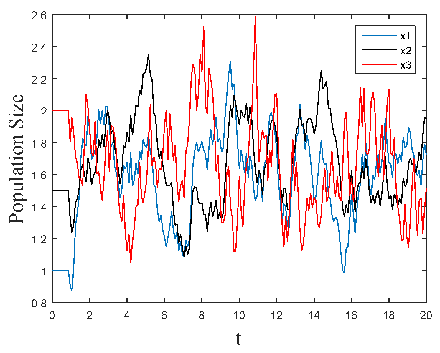
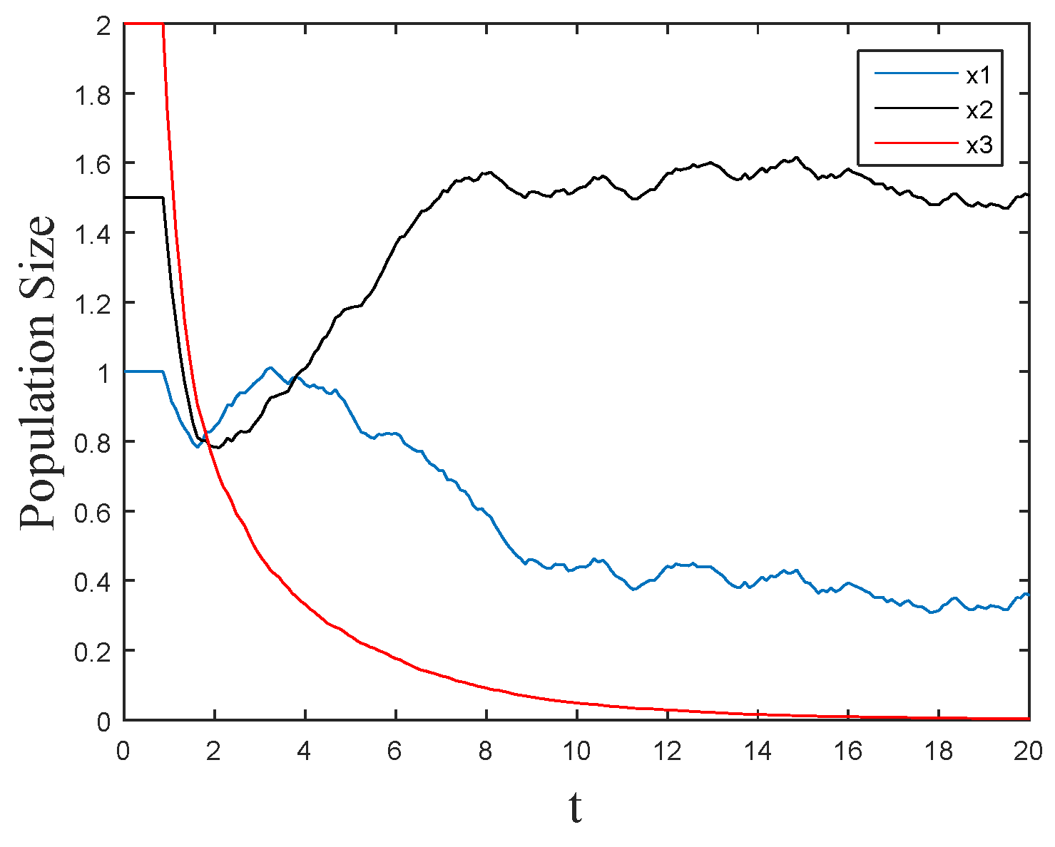
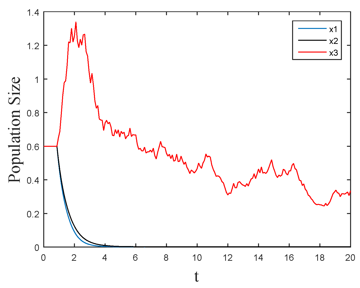
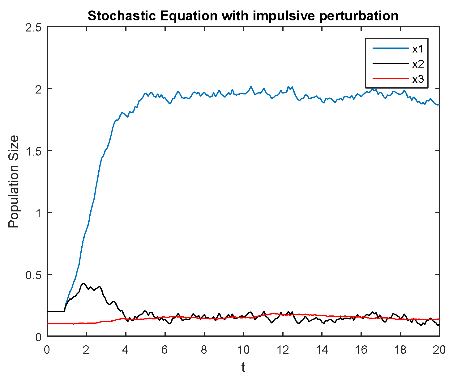
5. Numerical Examples

Case 1. For Model (2), set the initial value ${(x_{10},x_{20},x_{30})}^T={(0.4,0.6,0.5)}^T$. Choose the parameter $r_1=1.2$, $r_2=1$, $r_3=1$, $a_{11}=0.3$, $a_{12}=0.2$, $a_{21}=0.12$, $a_{22}=0.22$, $a_{23}=0.25$, $a_{32}=1$, $a_{33}=0.6$, ${\sigma }_1=0.001$, ${\sigma }_2=0.001$, ${\sigma }_3=0.5$, ${\alpha }_{1k}=0$, ${\alpha }_{2k}=0$, ${\alpha }_{3k}=e^{\frac{1}{k^2}}-1$, $t_k=k$, ${\tau }_{ij}\left(t\right)=0.2+0.2sint$. $R_1=r_1+{\sum }_{j=1}^{k}ln(1+{\alpha }_{1j})=1$, $R_2=-1$, $R_3=-r_3+{\sum }_{j=1}^{k}ln(1+{\alpha }_{3j})<-1+\frac{{\pi }^2}{6}<0.71$. $A_1=-1$, $A_2=-1$, $0<A_3=\frac{{\prod }_{t_k<t}{e}^{\frac{1}{j^2}}}{{\left({\prod }_{j=1}^k{e}^{\frac{1}{j^2}}\right)}^t}<e^{{\sum }_{t_k<t}\frac{1}{j^2}}<e^{\frac{{\pi }^2}{6}}<5.2$, $\frac{1}{2}({\sigma }_1^2+{\sigma }_2^2+{\sigma }_3^2)<0.13$, $R_1+R_2+R_3=-1.29$. $D<0$. From Theorem 3, all the species are 1st moment extinction, shown in Figure 1.

Case 2. For Model (2), set the initial value ${(x_{10},x_{20},x_{30})}^T={(1,1.5,2)}^T$. Choose the parameter $r_1=1$, $r_2=1$, $r_3=0.2$, $a_{11}=0.22$, $a_{12}=0.7$, $a_{21}=0.1$, $a_{22}=0.2$, $a_{23}=0.51$, $a_{32}=0.22$, $a_{33}=0.5$, ${\sigma }_1=1$, ${\sigma }_2=2$, ${\sigma }_3=1$, ${\alpha }_{1k}=0$, ${\alpha }_{2k}=0$, ${\alpha }_{3k}=e^{\frac{1}{k^2}}-1$, $t_k=k$, ${\tau }_{ij}\left(t\right)=0.2+0.2sint$, $R_1=r_1+{\sum }_{j=1}^{k}ln(1+{\alpha }_{1j})=0.6$, $R_2=r_2+{\sum }_{j=1}^{k}ln(1+{\alpha }_{1j})=-0.3$, $R_3=-r_3+{\sum }_{j=1}^{k}ln(1+{\alpha }_{1j})=-0.1+\frac{{\pi }^2}{6}<1.61$, $A_1=-1$, $A_2=-1$, $0<A_3=<5.2$, $\frac{1}{2}({\sigma }_1^2+{\sigma }_2^2+{\sigma }_3^2)=1.5$, $D>0$. All the species are 1st moment persistence by Theorem 3. Figure 2 illustrate this.

In Figure 3, we use the same data from Case 2 to reduce the intensity of white noise, the top predator tends to go extinct. We find that moderate noise intensity is good for the balance of the whole ecosystem. When white noise is too low, it is not conducive to the survival of the top predator.

Remark 4. 

Using the data in 2, we set ${\sigma }_1={\sigma }_2={\sigma }_3=0.1$. In deterministic Model (1), the equilibrium $(\frac{b_1}{c_{11}},0,0)$ always exists. That is, prey can survive without a predator and the predators cannot survive without prey. When there is only prey in the deterministic system in Figure 4, it can survive for a long time to reach the same point as in [1]. When white noise is added to the system, intermediate and top predators change from extinct state to persistent state in Figure 5. Therefore, in this system, white noise is beneficial to the balance of the entire ecosystem, which is more general than Mao’s results in [40]. That is to say, environmental noise inhibits the explosion in population dynamics and keeps the ecosystem in balance.

Remark 5. 

If the pulse intensity is bounded, the impulsive perturbations do not affect the persistence and extinction of the population in time average. The environmental stochastic perturbation on the prey and predator affects the persistence and extinction of the population.

6. Conclusions

This paper investigates a class of autonomous impulsive stochastic food chain system with time-varying delays. Appropriate white noise is conducive to the balance of the entire ecosystem. That is to say, environmental noise inhibits the explosion in population dynamics and keeps the ecosystem in balance. When the Razumikhins condition holds, the exponential stability and practical exponential stability of species are independent of time delay. Studying steady-state distribution, persistence and extinction of populations is also very important to obtain directions for future study.

References

1. Yang, Q.; Zhang, X.; Jiang, D. Dynamical Behaviors of a Stochastic Food Chain System with Ornstein—Uhlenbeck Process. J. Nonlinear Sci. 2022, 32, 34. [Google Scholar] [CrossRef]
2. Qiu, H.; Dong, W. Stationary distribution and global asymptotic stability of a three Stationary distribution and global asymptotic stability of a threespecies stochastic food-chain system. Turk. J. Math. 2017, 41, 5. [Google Scholar] [CrossRef]
3. Gabriele, V.; Antonello, P. On-Off Intermittency in a Three-Species Food Chain. Mathematics 2021, 9, 1641. [Google Scholar]
4. Bahar, A.; Mao, X. stochastic delay Lotka-Volterra model. J. Math. Anal. Appl. 2004, 292, 364–380. [Google Scholar] [CrossRef] [Green Version]
5. Wu, J. Stability of a three-species stochastic delay predator-prey system with Lvy noise. Phys. A 2018, 502, 492–505. [Google Scholar] [CrossRef]
6. Rui, H.; Zou, X.; Wang, K. Asymptotic behavior of a stochastic non-autonomous predator-prey model with impulsive perturbations. Commun. Nonlinear Sci. Numer. Simul. 2015, 20, 965–974. [Google Scholar]
7. Ahmad, S.; Stamova, I. Almost necessary and sufficient conditions for survival of species. Nonlinear Anal. Real World Appl. 2004, 5, 219–229. [Google Scholar] [CrossRef]
8. Freedman, H.; Waltman, P. Mathematical analysis of some three-species food-chain models. Math. Biosci. 1977, 33, 257–276. [Google Scholar] [CrossRef]
9. Bainov, D.; Simeonov, P. Impulsive Difffferential Equations Periodic Solutions and Applications; Longman: Harlow, UK, 1993. [Google Scholar]
10. Li, X.; Cao, J. An Impulsive Delay Inequality Involving Unbounded Time-Varying Delay and Applications. IEEE Trans. Autom. Control 2017, 62, 3618–3625. [Google Scholar] [CrossRef]
11. Lu, C.; Chen, J.; Fan, X.; Zhang, L. Dynamics and simulations of a stochastic predator-prey model with infinite delay and impulsive perturbations. J. Appl. Math. Comput. 2017, 57, 437–465. [Google Scholar] [CrossRef]
12. Rao, R.; Lin, Z.; Ai, X.; Wu, J. Synchronization of Epidemic Systems with Neumann Boundary Value under Delayed Impulse. Mathematics 2022, 10, 2064. [Google Scholar] [CrossRef]
13. Ahmad, S.; Stamova, I.M. Asymptotic stability of competitive systems with delays and impulsive perturbations. J. Math. Anal. Appl. 2007, 334, 686–700. [Google Scholar] [CrossRef]
14. Alzabut, J.O.; Abdeljawad, T. On existence of a globally attractive periodic solution of impulsive delay logarithmic population model. Appl. Math. Comput. 2008, 198, 463–469. [Google Scholar] [CrossRef]
15. He, M.; Chen, F. Dynamic behaviors of the impulsive periodic multi-species predator–prey system. Comput. Math. Appl. 2009, 57, 248–265. [Google Scholar] [CrossRef] [Green Version]
16. Hou, J.; Teng, Z.; Gao, S. Permanence and global stability for nonautonomous N-species Lotka-Volterra competitive system with impulses. Nonlinear Anal. Real World Appl. 2015, 11, 1882–1896. [Google Scholar] [CrossRef]
17. Baek, H. A food chain system with Holling type IV functional response and impulsive perturbations. Comput. Math. Appl. 2010, 60, 1152–1163. [Google Scholar] [CrossRef] [Green Version]
18. Wang, Q.; Zhang, Y.; Wang, Z.; Ding, M.; Zhang, H. Periodicity and attractivity of a ratio-dependent Leslie system with impulses. J. Math. Anal. Appl. 2011, 376, 212–220. [Google Scholar] [CrossRef] [Green Version]
19. Liu, M.; Wang, K. On a stochastic logistic equation with impulsive perturbations. Comput. Math. Appl. 2012, 63, 871–886. [Google Scholar] [CrossRef] [Green Version]
20. Zuo, W.; Jiang, D. Periodic solutions for a stochastic non-autonomous Holling–Tanner predator–prey system with impulses. Nonlinear Anal. Hybrid Syst. 2016, 22, 191–201. [Google Scholar] [CrossRef]
21. Lu, C.; Ding, X. Persistence and extinction of a stochastic logistic model with delays and impulsive perturbation. Acta Math. Sci. 2014, 34, 1551–1570. [Google Scholar] [CrossRef]
22. Yao, Q.; Lin, P.; Wang, L.; Wang, Y. Practical Exponential Stability of Impulsive Stochastic Reaction–Diffusion Systems with Delays. IEEE Trans. Cybern. 2020, 52, 2687–2697. [Google Scholar] [CrossRef] [PubMed]
23. Zhao, Y.; Wang, L.; Wang, Y. The Periodic Solutions to a Stochastic Two-Prey One-Predator Population Model with Impulsive Perturbations in a Polluted Environment. Methodol. Comput. Appl. Probab. 2021, 23, 859–872. [Google Scholar] [CrossRef]
24. Hu, W.; Zhu, Q. Moment exponential stability of stochastic nonlinear delay systems with impulse effects at random times. Int. J. Robust Nonlinear Control 2018, 29, 3809–3820. [Google Scholar] [CrossRef]
25. Wang, Q.; Liu, X. Impulsive stabilization of delay differential systems via the Lyapunov–Razumikhin method. Appl. Math. Lett. 2007, 20, 839–845. [Google Scholar] [CrossRef] [Green Version]
26. Yang, Z.; Xu, D. Stability Analysis and Design of Impulsive Control Systems with Time Delay. IEEE Trans. Autom. Control 2007, 52, 1448–1454. [Google Scholar] [CrossRef]
27. Guo, Y.; Zhu, Q.; Wang, F. Stability analysis of impulsive stochastic functional differential equations. Commun. Nonlinear Sci. Numer. Simul. 2019, 82, 105013. [Google Scholar] [CrossRef]
28. Cheng, P.; Deng, F.; Yao, F. Exponential stability analysis of impulsive stochastic functional differential systems with delayed impulses. Commun. Nonlinear Sci. Numer. Simul. 2014, 19, 2104–2114. [Google Scholar] [CrossRef]
29. Cheng, P.; Deng, F.; Yao, F. Almost sure exponential stability and stochastic stabilization of stochastic differential systems with impulsive effects. Nonlinear Anal. Hybrid Syst. 2018, 30, 106–117. [Google Scholar] [CrossRef]
30. Peng, S.; Jia, B. Some criteria on p-th moment stability of impulsive stochastic functional differential equations. Stat. Probab. Lett. 2010, 80, 1085–1092. [Google Scholar] [CrossRef]
31. Peng, S.; Zhang, Y. Razumikhin-Type Theorems on pth Moment Exponential Stability of Impulsive Stochastic Delay Differential Equations. IEEE Trans. Autom. Control 2010, 55, 1917–1922. [Google Scholar] [CrossRef]
32. Hu, W.; Zhu, Q.; Karimi, H.R. Some Improved Razumikhin Stability Criteria for Impulsive Stochastic Delay Differential Systems. IEEE Trans. Autom. Control 2019, 64, 5207–5213. [Google Scholar] [CrossRef]
33. Hu, W.; Zhu, Q. Stability analysis of impulsive stochastic delayed differential systems with unbounded delays. Syst. Control. Lett. 2020, 136, 104–606. [Google Scholar] [CrossRef]
34. Lu, C.; Ding, X. Persistence and extinction of an impulsive stochastic logistic model with infinite delay. Osaka J. Math. 2018, 53, 1–29. [Google Scholar]
35. Caraballo, T.; Hammami, M.A.; Mchiri, L. Practical Asymptotic Stability of Nonlinear Stochastic Evolution Equations. Stoch. Anal. Appl. 2013, 32, 77–87. [Google Scholar] [CrossRef] [Green Version]
36. Caraballo, T.; Hammami, M.A.; Mchiri, L. On the practical global uniform asymptotic stability of stochastic differential equations. Stochastics 2016, 88, 45–56. [Google Scholar] [CrossRef]
37. Caraballo, T.; Hammamib, M.; Mchirib, L. Practical exponential stability of impulsive stochastic functional differential equations. Syst. Control Lett. 2017, 109, 43–48. [Google Scholar] [CrossRef]
38. Peng, S.; Zhu, X. Necessary and sufficient condition for comparison theorem of 1- dimensional stochasti cdifferential equations. Stoch. Process. Appl. 2006, 116, 370–380. [Google Scholar] [CrossRef] [Green Version]
39. Hung, L.C. Stochastic delay population systems. Appl. Anal. 2009, 88, 1303–1320. [Google Scholar] [CrossRef]
40. Mao, X.; Marion, G.; Renshaw, E. Environmental Brownian noise suppresses explosion in population dynamics. Stoch. Process Appl. 2002, 97, 95–110. [Google Scholar] [CrossRef]
Figure 1. The solution to x i , i = 1 , 2 , 3 are 1st moment extinction.
Mathematics 11 00147 g001
Figure 2. The solution to x i , i = 1 , 2 , 3 are 1st moment persistence.
Mathematics 11 00147 g002
Figure 3. Other data are the same as in Case 2, and the intensity of white noise is reduced.
Mathematics 11 00147 g003
Figure 4. The deterministic system.
Mathematics 11 00147 g004
Figure 5. Increasing the intensity of white noise.
Mathematics 11 00147 g005
Disclaimer/Publisher’s Note: The statements, opinions and data contained in all publications are solely those of the individual author(s) and contributor(s) and not of MDPI and/or the editor(s). MDPI and/or the editor(s) disclaim responsibility for any injury to people or property resulting from any ideas, methods, instructions or products referred to in the content.