Andness Directedness for t-Norms and t-Conorms

Abstract

Tools for decision making need to be simple to use. In previous papers, we advocated that decision engineering needs to provide these tools, as well as a list of necessary properties that aggregation functions need to satisfy. When we model decisions using aggregation functions, andness-directedness is one of them. A crucial aspect in any decision is the degree of compromise between criteria. Given an aggregation function, andness establishes to what degree the function behaves in a conjunctive manner. That is, to what degree some criteria are mandatory. Nevertheless, from an engineering perspective, what we know is that some criteria are strongly required and we cannot ignore a bad evaluation even when other criteria are correctly evaluated. That is, given our requirements of andness, what are the aggregation functions we need to select. Andness is not only for mean-like functions, but it also applies to t-norms and t-conorms. In this paper, we study this problem and show how to select t-norms and t-conorms based on the andness level.

1. Introduction

Aggregation functions [1] play an important role in any decision-making process [2]. We have aggregation functions in multicriteria decision making and in multiobjective decision making. Recall that the former is understood to be the case of a finite set of alternatives and the latter to correspond to the case of an infinite set of alternatives.

In both cases, alternatives are evaluated into a set of criteria and the goal is to find a good or optimal alternative satisfying the criteria. It is well known that the difficulty of the problem is due to the fact that criteria are conflicting and, thus, we need to have an overall good performance of the alternative, but an absolute good performance on all criteria is usually not possible. Pareto efficient solutions (i.e., solutions in the Pareto front), and solutions that reach a good compromise play then a role.

When not all criteria are going to be satisfied, aggregation has a very important role. It is a way to model the compromise between criteria. For this reason, families of aggregation functions [1,3,4,5] have been defined. Most families of functions require parameters. Different aggregation functions will produce different orderings on the alternatives, the same applies to different parameterizations for a given function. Therefore, this means that we need to select in an appropriate way both the aggregation function and its parameters.

In a recent paper [6] (see also [7]), we described ten necessary properties that aggregation functions are required to satisfy for decision engineering. They are (P1) semantic identity of arguments, (P2) andness/orness-directedness and andness/orness monotonicity, (P3) aggregation in the full range from drastic conjunction to drastic disjunction, (P4) selectable idempotency/nonidempotency, (P5) selectable support for annihilators, (P6) adjustable threshold andness/orness, (P7) selectable commutativity/noncommutativity based on importance weights, (P8) unrestricted usability in a soft computing propositional calculus, (P9) independence of importance and simultaneity/substitutability, (P10) applicability based on simplicity, specifiability, and readability of aggregators.

In this paper, we focus on P2, that is, andness/orness-directedness. Andness and orness were defined by Dujmović [8,9] as the level of simultaneity and substitutability of the aggregation. In other words, a high orness permits that a bad criteria be compensated by a good one. On the other hand, a high andness requires both criteria to be satisfied to a great degree. Andness and orness are related and add up to one. Dujmović proposed and studied andness and orness for several functions [8,9,10,11] and a number of inputs (as the andness depends on how many values we aggregate). Yager introduced an expression for OWA [12]. We later studied [13,14] the case of WOWA (Weighted OWA [15]). Andness-directedness is about selection of a function or its parameters from the andness level. This andness-directedness appears in [10]. It was later studied by O’Hagan [16,17] for the OWA. In the case of OWA, the goal is to find OWA weights that satisfy a given andness/orness, using entropy to select among all those vector of weights with the same andness. Carbonell et al. [18] and Fuller and Majlender [19,20] also studied this problem. We have studied the case of andness-directed OWA and WOWA in [21]. More concretely, we consider the family of generalized WOWA, which allows annihilators, and study how we can set all parameters given a certain value for andness. Andness-directedness for other aggregation functions can also be found in [2]. Parametric characterization of aggregation functions as proposed by [22] is similar to the idea of andness-directedness.

Aggregation is usually performed by means and related functions that satisfy the internality principle. That is, functions that return a value between the minimum and the maximum of the values being aggregated. This corresponds [2] to andness and orness between 0 and 1. Nevertheless, in some cases, we need to consider stronger functions in the sense that the outcome of an aggregation is less than the minimum or it is larger than the maximum. Fuzzy logic provides these type of operators, they are called t-norms and t-conorms. The minimum is an example of t-norm, but another one is product, and it is easy to see that $xy\le min(x,y)$. That is, product is still more conjunctive than minimum. Because of this relationship, while minimum has an andness equal to one, product has an andness that is larger than one (equal to 5/4 for two inputs). A similar idea appears in [23] were bounded extreme conformity is defined for aggregation functions.

In this paper, we show how to select an appropriate t-norm for a given andness. That is, an andness-directed selection of the t-norm. For this, instead of considering a (finite) set of t-norms and discussing their andness, we will consider a family of t-norms that are parameterized by a parameter and show how to tune this parameter given an andness level.

The structure of the paper is as follows. In Section 2, we introduce some basic definitions that we need in the rest of the paper. This includes the definition of t-norm and t-conorm, as well as some families of measures. We also review the formal definition of andness and orness. Then, in Section 3 we introduce our approach for andness-directed selection of t-norms. The paper finishes with some discussion and directions for future research.

2. Preliminaries

We have divided this section in two parts. The first one is about t-norms and some families of t-norms that are useful in our work. Then, we focus on andness and orness. For more details on t-norms and t-conorms, the books by Alsina et al. [24] and Klement et al. [25] are good reference works.

2.1. Fuzzy Operators: t-Norms and t-Conorms

In fuzzy sets theory, conjunction is modeled in terms of t-norms. They are functions ⊤ from $[0,1]\times [0,1]$ into [0, 1] that satisfy the following four properties.

• $\top (a,b)=\top (b,a)$ (commutativity)
• $\top (a,b)\le \top (c,d)$ when $a\le c$ and $b\le d$ (monotonicity)
• $\top (a,\top (b,c\left)\right)=\top (\top (a,b),c)$ (associativity)
• $\top (a,1)=a$ (identity)

It is easy to see that conjunction in logic (i.e., and) satisfies these properties. Thus, they imply a generalization of classical conjunction (which is defined in $\{0,1\}\times \{0,1\}$) in the fuzzy setting (i.e., in $[0,1]\times [0,1]$). Any t-norm ⊤ when values are restricted to be either 0 or 1 behaves just as the standard conjunction.

The most typical example of t-norm functions is the minimum, but the product is also a very much used t-norm in, for example, fuzzy control [26] because of its nonlinearity. Nevertheless, there are several other t-norms and, in particular, some families of t-norms. We will review some of them below. We select families that are parameterized and that the parameter permits us to select a t-norm between the minimum and the drastic t-norm. We describe the t-norms in their binary form. These functions are associative and expressions for $n>2$ inputs can be built.

Let $T_{mn}$ denote the minimum, $T_{ap}$ the algebraic product, $T_{bd}$ the bounded difference, and let $T_{dr}$ denote the drastic intersection. That is, $T_{mn}(a,b)=min(a,b)$, $T_{ap}(a,b)=ab$, $T_{bd}(a,b)=max(0,a+b-1)$, and

$$T_{dr}=\left\{\begin{array}{cc}a& \mathrm{if}b=1\\ b& \mathrm{if}a=1\\ 0& \mathrm{otherwise}\end{array}\right.$$

Then for any t-norm ⊤, we have that

$$T_{dr}(a,b)\le \top (a,b)\le T_{mn}(a,b).$$

That is why we have interest in considering families of t-norms that cover the whole spectrum of t-norms.

We have described t-norms above. Similarly, we have that a t-conorm generalizes the disjunction in classical logic. A t-conorm ⊥ from $[0,1]\times [0,1]$ into $[0,1]$ is a function that satisfies the following four properties. Observe that the only one that changes from the properties above is the identity.

• $\perp (a,b)=\perp (b,a)$ (commutativity);
• $\perp (a,b)\le \perp (c,d)$ when $a\le c$ and $b\le d$ (monotonicity);
• $\perp (a,\perp (b,c\left)\right)=\perp (\perp (a,b),c)$ (associativity);
• $\perp (a,0)=a$ (identity).

While t-norms are often denoted by T, t-conorms are often denoted by S. We will use this notation for particular families of t-norms. It is relevant to observe that given t-norm T, $S(a,b)=1-T(1-a,1-b)$ is its dual t-conorm.

The typical disjunction is the maximum, but, again, there are alternatives to the use of maximum, and several families of parametric t-conorms exist. In a way similar to the case of t-norms, we will consider functions that range between maximum and drastic disjunction. We denote these t-conorms by $S_{mx}$ and $S_{dd}$. Analogous to the case of t-norms, we have that for any t-conorm ⊥, the following holds:

$$S_{mx}(a,b)\le \perp (a,b)\le S_{dd}(a,b).$$

In the rest of this section, we will review families of norms by Dombi, by Schweizer and Sklar (3 families) and by Yager. These families, as well as other examples of t-norms and t-conorms, are described in the excellent book by Klir and Yuan [27].

Dombi [28] introduced the following family of t-norms and t-conorms (for $\lambda >0$):

$$T_D(a,b;\lambda )={\left\{1+{\left[{\left(\frac{1}{a}-1\right)}^{\lambda }+{\left(\frac{1}{b}-1\right)}^{\lambda }\right]}^{1/\lambda }\right\}}^{-1}$$

$$S_D(a,b;\lambda )={\left\{1+{\left[{\left(\frac{1}{a}-1\right)}^{-\lambda }+{\left(\frac{1}{b}-1\right)}^{-\lambda }\right]}^{-1/\lambda }\right\}}^{-1}.$$

Note that for a and b equal to zero and one, they are defined according to the axioms for t-norms and t-conorms above. The same applies to the other families of norms discussed below.

It is worth mentioning that with respect to the t-norm, when $\lambda$ converges to 0, $T_D$ tends to the drastic intersection; when $\lambda =1$, $T_D$ converges to $ab/(a+b-ab)$; and when $\lambda$ converges to ∞, $T_D$ converges to $min(a,b)$.

With respect to the t-conorm, when $\lambda$ converges to 0, $S_D$ tends to the drastic disjunction; when $\lambda =1$, $S_D$ converges to $(a+b-2ab)/(1-ab)$; and when $\lambda$ converges to ∞, $S_D$ converges to $max(a,b)$.

Schweizer and Sklar [29] introduced several families of t-norms and t-conorms, some of which are also appropriate for our purpose. We review below these pairs of functions. Klir and Yuan [27] denote them as the first, second, and third family of norms. A fourth family is also described in Klir and Yuan’s book, but we do not review it here because it does not reach the drastic intersection.

The first family of Schweizer and Sklar is defined as follows (for $p\ne 0$):

$$T_{SS1}(a,b;p)={\left\{max(0,a^p+b^p-1)\right\}}^{1/p},$$

$$S_{SS1}(a,b;p)=1-{\left(max\left(0,{(1-a)}^p+{(1-b)}^p-1\right)\right)}^{1/p}.$$

With respect to the t-norm, when p converges to $-\infty$, $T_{SS1}$ converges to $min(a,b)$; when $p=1$, $T_{SS1}$ is $max(0,a+b-1)$; when p converges to zero, $T_{SS1}$ tends to $ab$; when $p=-1$, $T_{SS1}$ is $ab/(a+b-ab)$; when p converges to ∞, $T_{SS1}$ converges to the drastic intersection.

The second family is defined as follows (for $p>0$):

$$T_{SS2}(a,b;p)=1-{\left[{(1-a)}^p+{(1-b)}^p-{(1-a)}^p{(1-b)}^p\right]}^{1/p},$$

$$S_{SS2}(a,b;p)={\left(a^p+b^p-\left(a^p\right)\left(b^p\right)\right)}^{1/p}.$$

For the t-norm $T_{SS2}$, when p converges to zero, $T_{SS2}$ converges to the drastic intersection; when $p=1$, $T_{SS2}$ converges to $ab$; when p converges to ∞, $T_{SS2}$ converges to $min(a,b)$.

The third family is defined as follows (for $p>0$):

$$T_{SS3}(a,b;p)=e^{-{\left(\right|lna|}^p+{\left|lnb\right|}^p{)}^{1/p}},$$

$$S_{SS3}(a,b;p)=1-exp\left(-{\left(\right|\left(ln(1-a)\right|)}^p+{\left(\right|ln(1-b)\left|\right)}^p{)}^{1/p}\right).$$

For $T_{SS3}$, when p converges to zero, $T_{SS3}$ converges to the drastic intersection; when $p=1$, $T_{SS3}$ converges to $ab$; when p converges to ∞, $T_{SS3}$ converges to $min(a,b)$.

We finish this review with the family of t-norms introduced by Yager [30]. Its definition (for $w>0$) follows.

$$T_Y(a,b;w)=1-min(1,{[{(1-a)}^w+{(1-b)}^w]}^{1/w}),$$

$$S_Y(a,b;w)=min\left(1,{(\left(a^w\right)+\left(b^w\right))}^{1/w}\right).$$

For this t-norm, when w converges to 0, $T_{SSY}$ converges to the drastic intersection; when $w=1$, $T_{SSY}(a,b;1)=max(0,a+b-1)$; and when w converges to ∞, $T_{SSY}$ tends to $min(a,b)$.

2.2. Andness and Orness

Andness and orness were introduced by Dujmović [8,9] as a degree of conjunction and disjunction. They are defined in terms of the similarity to minimum and maximum, respectively. More formally, if we are considering a function $\mathbb{C}$ with n inputs in [0, 1] then $D={[0,1]}^n$, and andness corresponds to

$$\mathit{andness}\left(\mathbb{C}\right)=\frac{{\int }_{D}maxxdx-{\int }_D\mathbb{C}\left(x\right)dx}{{\int }_{D}maxxdx-{\int }_{D}minxdx}$$

where the integral is, naturally, an n-dimensional integral and $x\in D$.

Then, andness is in the range $[-1/(n-1),n/(n-1\left)\right]$, for n inputs. When $n=2$, the range is naturally $[-1,2]$. When operators are between minimum and maximum, andness is for any number of inputs in the range $[0,1]$. Operators that can return values smaller than the minimum (as t-norms) or larger than the maximum (as t-conorms) will provide andness outside $[0,1]$, reaching the minimum and the maximum of the interval with drastic disjunction and drastic conjunction.

The orness can be defined similarly but in terms of the minimum. Then, it follows that andness and orness add to one. We will use $\alpha$ to denote andness and $\omega$ to denote orness. Then, $\alpha +\omega =1$. Duality between t-norms and t-conorms is propagated into andness and orness, as they exchange their values.

The andnesss can be computed for some functions analytically or, otherwise, it can be computed numerically. The computation needs to take into account the number of inputs n, as, in general, andness for a t-norm depends on the number of inputs. Numerical computation for $T_{mn}$, $T_{ap}$, $T_{bd}$, $T_{dr}$ and $S_{mx}$, $T_{as}$, $T_{bs}$, and $T_{dr}$ for two inputs result into the values described in

Table 1. Andness of some relevant t-norms and t-conorms.

t-norm	${\mathit{T}}_{\mathit{m}\mathit{n}}$	${\mathit{T}}_{\mathit{a}\mathit{p}}$	${\mathit{T}}_{\mathit{b}\mathit{d}}$	${\mathit{T}}_{\mathit{d}\mathit{r}}$
andness	1.000	1.250	1.500	2.000
t-conorm	$S_{mx}$	$S_{as}$	$S_{bs}$	$S_{dr}$
andness	0.000	−0.250	−0.500	−1.000

.

3. Andness Directedness for t-Norms

In order to provide andness directedness, we proceed as follows. First, we select a family of t-norms among the five ones described in Section 2.1. We will assume that the parameter of this t-norm (that we denote by ⊤) is p. This parameter corresponds, of course, to w, $\lambda$ or p itself, according to the description above. Then, we will use ${\top }_p$ to denote that p is the parameter of ⊤.

We describe below the construction of the relationship between the parameter of the aggregation and its andness, as well as the andness-directed selection of the parameter given andness. We describe the process for two inputs; we would proceed in a similar way for any number of inputs. Note that the andness of a t-norm depends on the number of inputs.

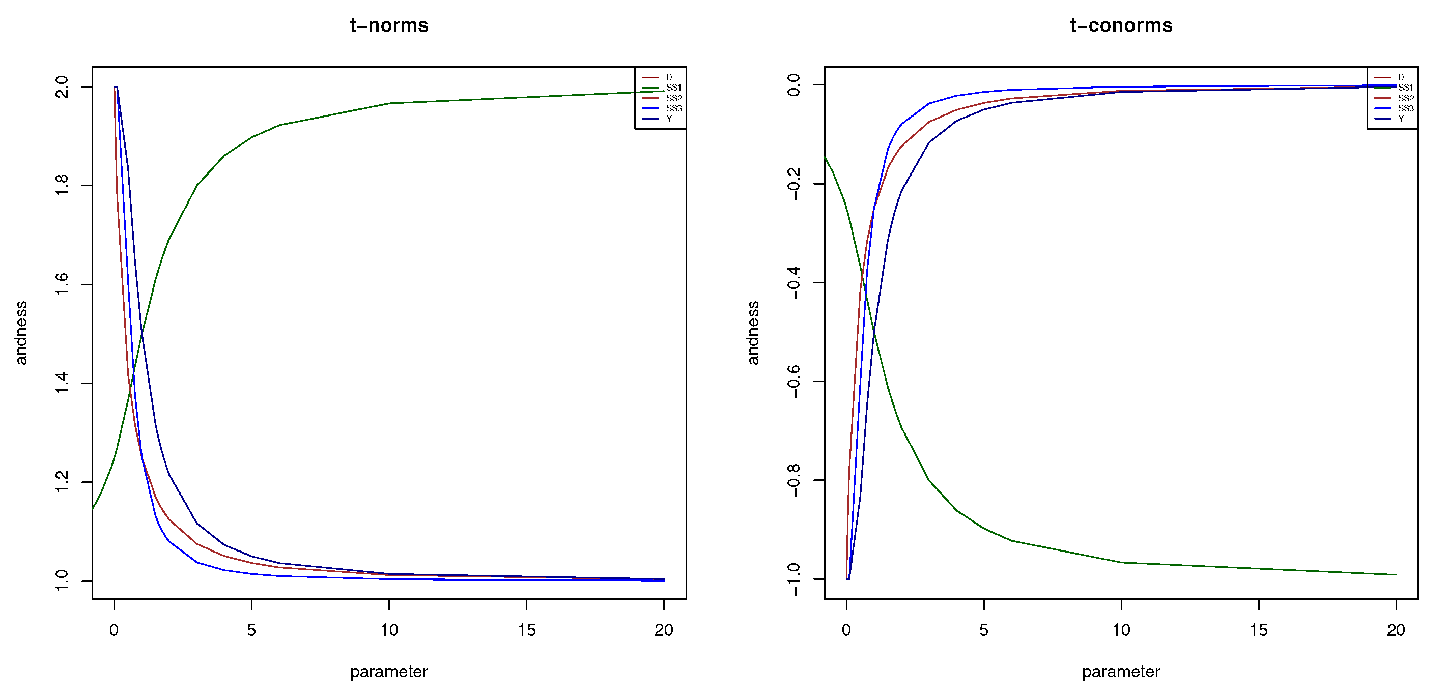
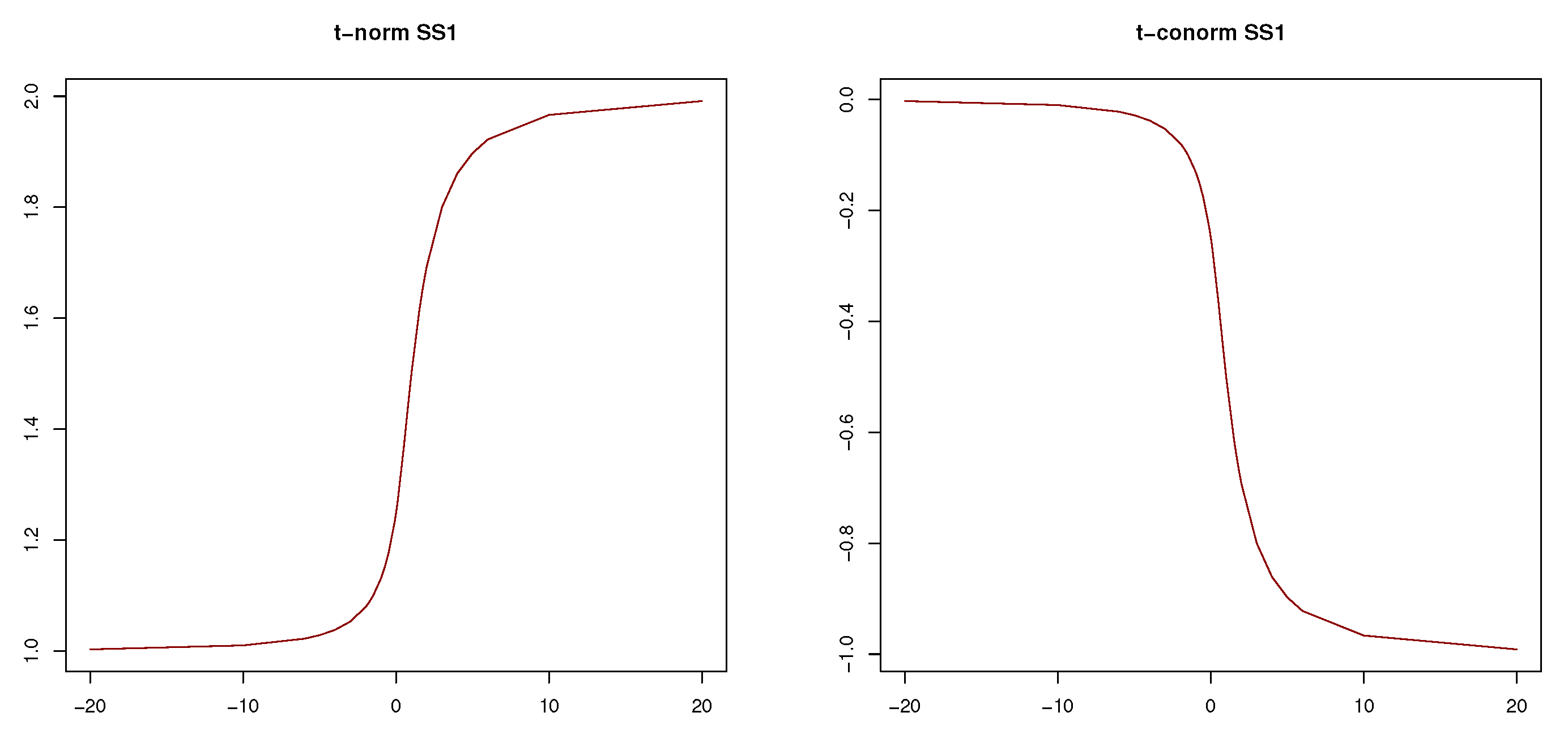
• Establish the relationship between the parameter and andness. Compute the andness of ${\top }_p$ for p in $range\left(p\right)$. As we cannot consider the full range of p, we will select a finite subset of this range large enough to have a good approximation. We denote this finite subset of the range by $R_p$. This process results in pairs ${\left\{(p,andness\left({\top }_p\right))\right\}}_{p\in R_p}$. As andness is monotonic with respect to p, we can interpolate (e.g., linearly) the relationship between p and the andness easily.
  Figure 1 displays the andness for the t-norms (left) and t-conorms (right) discussed in Section 2. Therefore, we include $T_D$, $T_{SS1}$, $T_{SS2}$, $T_{SS3}$, and $T_Y$ as t-norms, and $S_D$, $S_{SS1}$, $S_{SS2}$, $S_{SS3}$, $S_Y$ as t-conorms. It is worth noting that in the figure only four lines are visible because the lines for $T_D$ (Dombi’s t-norm) and $T_Y$ are indistinguishable. In Figure 1, we consider positive parameters $\lambda$, p, and w for all t-norms and t-conorms. We have discussed before that the parameter for both t-norm and t-conorm $T_{SS1}$ and $S_{SS1}$ can take any value except zero. For this reason, we represent the andness of these function independently in Figure 2.
• Establish the parameter given the andness. Given the andness level $\alpha$ and the pairs ${\left\{(p_i,{\alpha }_i)\right\}}_{i\in \{1,\cdots ,|R_p\left|\right\}}$ check if there is a value ${\alpha }_i=\alpha$. If this is the case, select $p_i$. Otherwise, find a pair of values ${\alpha }_i$ and ${\alpha }_{i+1}$ that satisfy ${\alpha }_i\le \alpha \le {\alpha }_{i+1}$. Then, first, compute $r=(\alpha -{\alpha }_i)/({\alpha }_{i+1}-{\alpha }_i)$ and, second, compute $p=p_i\ast (1-r)+p_{i+1}\ast r$. For example, given ${\alpha }_p=\alpha \left(p\right)=\mathit{andness}\left({\top }_p\right)$ for a given t-norm ⊤, we compute ${\alpha }_p^{-1}\left(\alpha \right)$, or, in other words, we approximate the parameter p as the inverse of the andness for the given andness $\alpha$.
  We will use $\lambda \left(\alpha \right)$, $p\left(\alpha \right)$, and $w\left(\alpha \right)$ to denote this process. For example, for $\alpha =1.5$, we obtain the following 5 parameters. For $T_D$, $\lambda =0.4143849$; for $T_{SS1}$, $p=0.9999819$; $T_{SS2}$, $p=0.4080617$; $T_{SS3}$$p=0.6143033$ and for $T_Y$, $w=1.0000$.

3.1. Differences between t-Norms for a Given Andness

Andness-directedness permits to align the parameters of t-norms so that they have the same conjunctive behavior. Then, we want to understand to what extent these t-norms differ. To do so, we compute the difference between them.

To compute the difference between two t-norms ${\top }_1$ and ${\top }_2$, possibly parameterized with parameters p and q, we consider the following expression.

$$\mathit{diff}({\top }_1^p,{\top }_2^q)={\int }_{[0,1]}{\int }_{[0,1]}\left|abs\right({\top }_1^p(x,y)-{\top }_2^q(x,y)|dxdy$$

This expression permits to compute the difference between two t-norms ${\top }_1$ and ${\top }_2$ for a given andness $\alpha$. To do this, first we find the parameter of ${\top }_1$ which corresponds to andness $\alpha$ and the same for ${\top }_2$. Let $p\left(\alpha \right)$ be the parameter of ${\top }_1$ which leads to andness $\alpha$ and let $q\left(\alpha \right)$ be the parameter of ${\top }_2$ which leads to the same andness. Then, we use the expression above to compute $\mathit{diff}({\top }_1^{p\left(\alpha \right)},{\top }_2^{q\left(\alpha \right)})$.

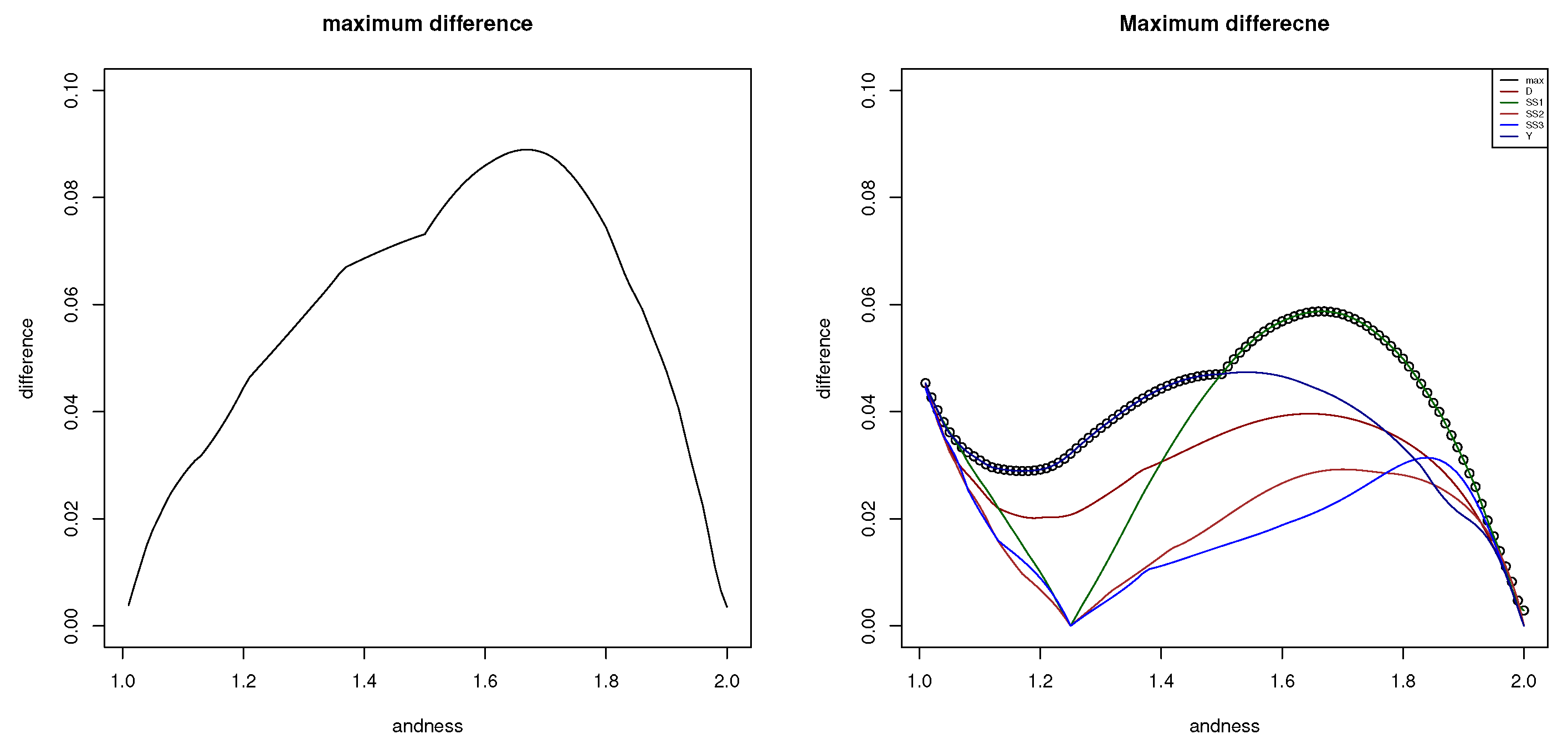
We have considered all pairs of t-norms with ⊤ being any of the $T_D$, $T_{SS1}$, $T_{SS2}$, $T_{SS3}$, and $T_Y$. This corresponds to 10 pairs of differences. In Figure 3 (left), we show the maximum of all differences. That is, the figure plots

$$max\mathit{diff}\left(\alpha \right)=\underset{{\top }_1,{\top }_2}{max}\mathit{diff}({\top }_1^p,{\top }_2^q).$$

We can see that the maximum is below 0.10. More precisely, it is 0.08894.

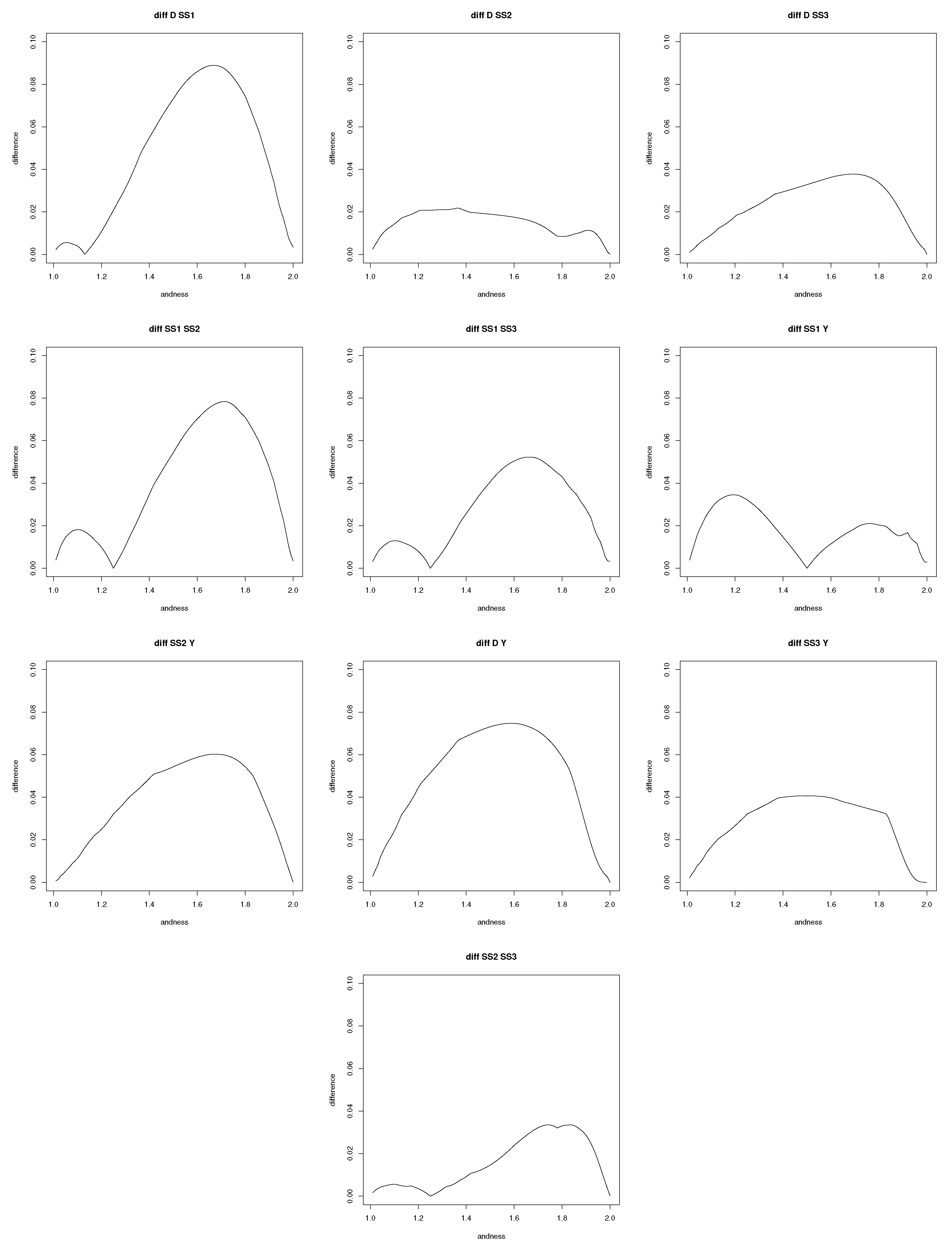
Figure 4 shows the results for each pair of t-norms. It can be observed that pairs that involve $T_{SS1}$ and $T_Y$ are the ones with a larger difference.

3.2. Differences between t-Norms and High Hyperconjunction for a Given Andness

We have also computed the difference between these t-norms and a high hyperconjunction (in the sense of Dujmović in [2]). High hyperconjunction has andness larger than 1 but, in general, it is not a t-norm. For example, associativity does not hold. More particularly, we consider the following expression, which corresponds to the weighted power function,

$$hC(a,b;p,q,\alpha )={\left(a^p·b^q\right)}^{\sqrt{3/(2-\alpha )}-1}.$$

Here, $\alpha$ refers to the andness level, and p and q are two weights that add up to 2 (i.e., two–this is not a typo). In our experiments, we use $p=q=1$. That is, the two inputs have the same weight.

Note that this definition is such that the andness of $hC$ for a given $\alpha$ is precisely $\alpha$. This function $hC$ does not lead to minimum for $\alpha =1$, so, our analysis focuses on $\alpha >1.25$ when the expression corresponds to the product. In [2] and related works, interpolation is used between minimum and the product for andness in the interval [1, 1.25].

The differences between t-norms and $hC$ are in Figure 3 (right). We can observe that maximum differences correspond to t-norms $T_{SS1}$ and $T_Y$. These were precisely the t-norms that also had maximum differences in the comparison between pairs of t-norms. Nevertheless, we can see that the hyperconjunction has a lower maximum difference.

3.3. Analysis

$T_{SS3}$ is the t-norm with the lowest maximum difference to all the others, and such difference is similar to the one of high hyperconjunction $hC$. The difference between $T_{SS3}$ and $hC$ is about 0.04.

We have also seen that $T_{SS1}$ and $T_Y$ are the t-norms that have largest difference from the others. We can observe that in their definitions we have either a minimum or maximum, which causes a discontinuity in the derivative and a flat region equal to zero in the norm. To compensate for these flat regions and have the same andness, the function should be larger in the non-zero regions.

To illustrate this, we consider the t-norm of (0.8, 0.8) and the t-norm of (0.5, 0.5) for an andness equal to $\alpha =1.6$. The results are presented in

Table 2. Computation of different t-norms with andness $\alpha =1.6$.

Case	${\mathit{T}}_{\mathit{D}}$	${\mathit{T}}_{\mathbf{SS}1}$	${\mathit{T}}_{\mathbf{SS}2}$	${\mathit{T}}_{\mathbf{SS}3}$	${\mathit{T}}_{\mathit{Y}}$
(0.8, 0.8)	0.3566074	0.5738743	0.4089883	0.4146452	0.5387788
(0.5, 0.5)	0.1217016	0	0.1120718	0.06492248	0

. We can observe that the norm of (0.5, 0.5) has a zero value for $T_{SS1}$ and $T_Y$ and a non-zero for the others larger than 0.1. In contrast, for (0.8, 0.8), all values are non-zero. In this case, for $T_{SS1}$ and $T_Y$, the value is significatively larger than for the other t-norms. As this is for fixed andness, this behavior is to compensate for the other lower results.

As a conclusion, $T_{SS3}$ and $hC$ seem to be good alternatives, being a kind of average conjunctions and being smooth, not suffering from the fact of a non-continuous derivative (i.e., avoiding the conjunction stronger in some regions and softer in others). $T_D$ and $T_{SS2}$ are also smooth but have larger differences with $T_{SS1}$ and $T_Y$.

Among $T_{SS3}$ and $hC$, only $T_{SS3}$ is a t-norm. Therefore, for andness-directed t-norms, $T_{SS3}$ seems the best alternative.

4. Conclusions and Future Directions

In this work, our goal was to study how to select a t-norm based on an andness level, that is, andness-directed t-norms. This problem has been made concrete by means of considering five families of parametric t-norms. That is, t-norms that depend on a parameter that permits to change their degree of conjunction.

Our experiments show that $T_{SS3}$, a family of t-norms defined by Schweizer and Sklar, seems to be a good family for this problem, as it has a soft behavior and is a kind of average t-norm in terms of its similarity to other t-norms.

We have described our approach for t-norms. The same applies to t-conorms. In fact, duality between t-norms and t-conorms, as well as the fact that $\alpha +\omega =1$, can be used for this purpose.

As future directions, we consider the analysis of other families of functions and consider andness-directedness together with other properties that may introduce constraints to the problem. For example, and said in different terms, we wonder if there are relevant properties that may imply that it is better to select $T_{SS1}$ instead of $T_{SS3}$.

References

- Torra, V.; Narukawa, Y. Modeling Decisions: Information Fusion and Aggregation Operators; Springer: Berlin/Heidelberg, Germany, 2007. [Google Scholar]
- Dujmović, J.J. Soft Computing Evaluation Logic; J. Wiley and IEEE Press: Hoboken, NJ, USA, 2018. [Google Scholar]
- Beliakov, G.; Pradera, A.; Calvo, T. Aggregation Functions: A Guide for Practitioners; Springer: Berlin/Heidelberg, Germany, 2008. [Google Scholar]
- Beliakov, G.; Bustince, H.; Calvo, T. A Practical Guide to Averaging Functions; Springer: Berlin/Heidelberg, Germany, 2016. [Google Scholar]
- Grabisch, M.; Marichal, J.-L.; Mesiar, R.; Pap, E. Aggregation Functions; Cambridge University Press: Cambridge, MA, USA, 2009. [Google Scholar]
- Dujmović, J.J.; Torra, V. Properties and comparison of andness-characterized aggregators. Int. J. Intel. Syst. 2021, 36, 1366–1385. [Google Scholar] [CrossRef]
- Dujmović, J.J.; Torra, V. Aggregation functions in decision engineering: Ten necessary properties and parameter-directedness. In Proceedings of the International Conference on Intelligent and Fuzzy Systems, Istanbul, Turkey, 24–26 August 2021; pp. 173–181. [Google Scholar]
- Dujmović, J.J. A generalization of some functions in continous mathematical logic–evaluation function and its applications. In Proceedings of the Informatica Conference, Bled, Yugoslavia; 1973. Paper d27 (In Serbo-Croatian). [Google Scholar]
- Dujmović, J.J. Two integrals related to means. J. Univ. Belgrade Dept. Ser. Math. Phys. 1973, 412–460, 231–232. [Google Scholar]
- Dujmović, J.J. Extended continuous logic and the theory of complex criteria. J. Univ. Belgrade EE Dept. Ser. Math. Phys. 1975, 498, 197–216. [Google Scholar]
- Dujmović, J.J. Weighted conjunctive and disjunctive means and their application in system evaluation. J. Univ. Belgrade EE Dept. Ser. Math. Phys. 1974, 483, 147–158. [Google Scholar]
- Yager, R.R. Families of OWA operators. Fuzzy Sets Syst. 1993, 59, 125–148. [Google Scholar] [CrossRef]
- Torra, V. Empirical analysis to determine Weighted OWA orness. In Proceedings of the 5th International Conference on Information Fusion (Fusion 2001), Montréal, QC, Canada, 26–29 March 2001. [Google Scholar]
- Torra, V. Effects of orness and dispersion on WOWA sensitivity. In Artificial Intelligence Research and Development; Alsinet, T., Puyol-Gruart, J., Torras, C., Eds.; IOS Press: Amsterdam, The Netherlands, 2008; pp. 430–437. ISBN 978-1-58603-925-7. [Google Scholar]
- Torra, V. The weighted OWA operator. Int. J. Intel. Syst. 1997, 12, 153–166. [Google Scholar] [CrossRef]
- O’Hagan, M. Fuzzy decision aids. In Proceedings of the 21st Annual Asilomar Conference on Signals, Systems, and Computers, Pacific Grove, CA, USA, 2–4 November 1987; IEEE and Maple Press: Piscataway, NJ, USA, 1988; Volume 2, pp. 624–628. [Google Scholar]
- O’Hagan, M. Aggregating template or rule antecedents in real-time expert systems with fuzzy set logic. In Proceedings of the 22nd Annual IEEE Asilomar Conference Signals, Systems, Computers, Pacific Grove, CA, USA, 31 October–2 November 1988; pp. 681–689. [Google Scholar]
- Carbonell, M.; Mas, M.; Mayor, G. On a class of monotonic extended OWA operators. In Proceedings of the 6th IEEE International Conference on Fuzzy Systems, Barcelona, Spain, 1–5 July 1997; pp. 1695–1699. [Google Scholar]
- Fullér, R.; Majlender, P. An analytic approach for obtaining maximal entropy OWA operator weights. Fuzzy Sets Syst. 2001, 124, 53–57. [Google Scholar] [CrossRef]
- Fullér, R.; Majlender, P. On obtaining minimal variability OWA operator weights. Fuzzy Sets Syst. 2003, 136, 203–215. [Google Scholar] [CrossRef]
- Torra, V. Andness directedness for operators of the OWA and WOWA families. Fuzzy Sets Syst. 2021, 414, 28–37. [Google Scholar] [CrossRef]
- Kolesárová, A.; Mesiar, R. Parametric characterization of aggregation functions. Fuzzy Sets Syst. 2009, 160, 816–831. [Google Scholar] [CrossRef]
- Jin, L.; Mesiar, R.; Yager, R.R. Families of value-dependent preference aggregation operators with their structures and properties. Int. J. Uncertain. Fuzziness-Knowl.-Based Syst. 2022, in press. [Google Scholar]
- Alsina, C.; Frank, M.J.; Schweizer, B. Associative Functions: Triangular Norms and Copulas; World Scientific: Singapore, 2006. [Google Scholar]
- Klement, E.P.; Mesiar, R.; Pap, E. Triangular Norms; Kluwer Academic Publisher: Philip Drive Norwell, MA, USA, 2000. [Google Scholar]
- Driankov, D.; Hellendoorn, H.; Reinfrank, M. An Introduction to Fuzzy Control; Springer: New York, NY, USA, 1993. [Google Scholar]
- Klir, G.J.; Yuan, B. Fuzzy Sets and Fuzzy Logic: Theory and Applications; Prentice Hall: London, UK, 1995. [Google Scholar]
- Dombi, J. A general class of fuzzy operators, the DeMorgan class of fuzzy operators and fuzziness measures induced by fuzzy operators. Fuzzy Sets Syst. 1982, 8, 149–163. [Google Scholar] [CrossRef]
- Schweizer, B.; Sklar, A. Associative functions and abstract semigroups. Publ. Math. Debr. 1963, 10, 69–81. [Google Scholar]
- Yager, R.R. On a general class of fuzzy connectives. Fuzzy Sets Syst. 1980, 4, 235–242. [Google Scholar] [CrossRef]
Figure 1.
Andness of t-norms , , , , (left) and t-conorms , , , , (right) in terms of their parameters (, p, or w).
Figure 2.
Andness of t-norm (left) and t-conorm (right) given its parameter p.
Figure 3.
Given andness , maximum difference between pairs of t-norms , , , , (left), and difference between high hyperconjunction and the same t-norms (right). The parameters of the t-norms (, p, or w) have been selected so that the t-norm has precisely andness (i.e., (, , and ).
Figure 4.
Given andness , difference between pairs of t-norms , , , , . Their parameters (, p, or w) have been selected so that the t-norm has precisely andness (i.e., (, , and ).