Dynamic Parameters Identification Method of 6-DOF Industrial Robot Based on Quaternion

Abstract

Identifying accurate dynamic parameters is of great significance to improving the control accuracy of industrial robots, but this area is relatively unexplored in the research. In this paper, a new algorithm for accurately identifying the dynamic parameters of a 6-degrees-of-freedom (DOF) robot is proposed by establishing a dynamic model. First, a multibody dynamic model of the robot is established, which can decouple the dynamic parameters of the rigid bodies that make up the robot. Decoupling is the basis of parameters identification. In order to ensure that the model is suitable for large-angle range motion and has good real-time performance, quaternion is used as the angle coordinate, and the model established thereby eliminates the singularity and improves the calculation efficiency. Second, the dynamic model is rewritten, and the dynamic parameters are separated as the parameters to be identified; thus, the parameters identification model is obtained. Furthermore, an identification algorithm based on the least-squares method is proposed, which can realize the accurate identification of dynamic parameters. The algorithm is verified by a simulation example. The results show that the value of the maximum absolute error of the identified parameters is −0.0264, and the maximum relative error is 0.031%, which proves the correctness and accuracy of the algorithm.

1. Introduction

At present, intelligent manufacturing and precision manufacturing have put forward high-precision requirements for industrial robots. Obtaining precise dynamic parameters (mass and principal moment of inertia) is necessary to achieve precise control [1,2], and it is also of great significance to the vibration reduction of the robot. Generally speaking, the dynamic parameters can be measured by physical experiments; that is, the mechanism to be tested is disassembled into various rigid bodies, the mass is obtained by weighing, and the principal moment of inertia is measured by the pendular motions [3]. However, to obtain the dynamic parameters of an industrial robot, it is necessary to apply the method of parameters identification. This is because industrial robots need high rigidity to ensure the stability of their working process and the processing quality, which makes industrial robots very heavy; furthermore, as a precision instrument, an industrial robot is not easy to disassemble. These two factors make it difficult to obtain the dynamic parameters of industrial robots by physical experiments.

There are two inverse problems in dynamics: one is control, and the other is parameters identification. The dynamics problem is to calculate the position, velocity and acceleration of the robot based on the joint forces and moments. The control problem is to calculate the joint force and torque according to the motion trajectory of the robot and its corresponding position, velocity and acceleration. Parameters identification uses an algorithm to solve the parameters to be identified by numerical analysis. In the algorithm, some parameters in the dynamic equation are taken as the parameters to be identified, and the other parameters are taken as the known parameters. Dynamic parameters identification is one kind of parameters identification, in which the particular parameters to be identified are dynamic parameters. Specifically, dynamic parameters identification is a computational method for solving dynamic parameters in momentum conservation equations or dynamic equations. Momentum conservation equations are only applicable to free-floating space robots, while ground-fixed robots require the use of dynamic equations [4]. The fundamental idea of parameters identification is to perform “input/output” analysis on the mathematical model that contains the dynamic parameters and to estimate the parameters’ values by minimizing the error between the real parameters and the dynamic parameters of the mathematical model. The calculated dynamic parameters have high accuracy [5]. There are many algorithms that can be used, such as least-squares method, gradient correction method, maximum likelihood method and prediction error method.

At present, compared with the research in the field of control, the research on parameters identification of robots is relatively undeveloped, and there are few related studies. Olsen et al. [6] studied the problem of identifying the velocity and acceleration according to the joint angle. The joint angle was measured by the encoder installed on the motor shaft, and thus, an identification method was proposed based on the maximum likelihood method. Gautier et al. [7] proposed an algorithm for identifying joint velocity and acceleration based on the least-squares method by measuring the joint forces and moments. The algorithm transformed the nonlinear least-squares problem into a linear problem by simplifying the dynamic model. The effectiveness of the algorithm was verified on a rigid 2-degrees-of-freedom (DOF) robot. Wang et al. [8] proposed an algorithm to identify the joint torque of a 6-DOF robot, and a deep neural network method was applied in the algorithm to compensate for the torque error introduced by uncertainty. The error of the identified torque was less than 6% of the maximum torque. Xu et al. [9] studied the identification of joint torque. The dynamic model was simplified by eliminating the parameters with a low identification degree, and then a joint torque identification algorithm was proposed. The verification experiments were carried out on the KUKA LBR iiwa14 R820 robot, and the results show that the algorithm can accurately identify the joint torque of the robot. Urrea et al. [10] established an Eulerian–Lagrange dynamic model based on the acceleration, velocity, position and voltage of the servo motor actuator and avoided calculating the torque of each joint. Based on the dynamic model, a parameters identification method was proposed. The parameters to be identified were nonlinear coupling terms, and the method was used for the SCARA robot with 5-DOF.

Dynamic parameters identification is a special case of parameters identification, and the existing research is more sparse for the following reasons. First, with the increase in the DOF of a robot, the number of variables and the complexity of the dynamic equations increase significantly, and the phenomenon of parameters coupling becomes more obvious. This makes it difficult for the traditional Newton–Euler method and Lagrange method to decouple the dynamic parameters as the parameters to be identified. Second, the solution of complex dynamic equations puts forward higher requirements for the rapid solution capability of a computer. To solve the dynamic parameters in real time relies on the computing power of the computer. Obstructed by the above two difficulties, the existing dynamic parameters identification methods mainly measure the parameters such as motor current, joint force and torque, and they use different calculation methods to estimate the nonlinear coupling term of dynamic parameters. Since only some of the parameters in the dynamic equation are sampled, the model is greatly simplified and is therefore more of an estimation method. Díaz-Rodríguez et al. [11] used the combination of inertia tensor, mass and the mass moments with respect to the center of gravity as the parameters to be identified, and they established the Gibbs–Appell dynamic equation. Furthermore, an identification algorithm based on the least-squares method was proposed. The algorithm was applied to a 3-DOF parallel robot, and the results show that the variance between the identified value and the true value is 0.596 to 8.22. Gaz et al. [12] proposed a method to identify the dynamic parameters of a Panda robot. The dynamic equations are established by the Lagrange method and the Newton–Euler method, respectively, and the inverse dynamic equation is obtained by taking the combination of mass, centroid position and inertia as the dynamic parameters to be identified. This method can be used to identify the nonlinear dynamic parameters of a Panda robot, and the identification algorithm is the least-squares method. Briot et al. [13] proposed a systematic approach to derive a dynamic parameters identification model for parallel robots. By making the robot track some reference trajectories with no load and sampling the data of motor current and joint position, the inertial parameters and drive gain of the robot are identified, and the inertial parameters are nonlinear terms of mass and position coordinates. Hardeman et al. [14] introduced a finite-element-based method that can automatically generate models with identifiable dynamic parameters. The combination of mass, torque and inertia tensor components is used as the parameter to be identified, and the identification method is the linear least-squares method.

The requirements of higher control accuracy and higher accuracy of dynamic parameters are proposed in intelligent manufacturing. These requirements urgently need to be addressed. Therefore, it is necessary to develop a new algorithm to accurately identify the dynamic parameters. The accuracy of the identification results depends on the accuracy of the dynamic model. The more accurate the model, the greater the number of variables and the more difficult the decoupling. The more DOFs a robot has, the greater the difficulty.

Based on the above difficulties, the problem of dynamic parameters identification of a 6-DOF industrial robot is studied in this paper, and a new algorithm based on a multibody dynamic model is proposed that can accurately identify the dynamic parameters. Compared with previous studies, this algorithm can decouple the dynamic parameters. Unlike the previous methods, which take the nonlinear mixture term of the dynamic parameters as the parameters to be identified, this algorithm can directly identify the dynamic parameters. In addition, the algorithm has good accuracy, and the identified dynamic parameters have low errors. Compared with the previous identification algorithms, three improvements have been made in this paper to achieve accurate identification of dynamic parameters. First, an accurate multibody dynamics model is established in this paper. The simplified dynamic model is adopted in the previous method, which is beneficial to reducing the amount of sampled data and the calculation amount of the identification algorithm, and the corresponding identification algorithm can be used to solve some specific problems. When the parameters to be identified are few or are only strongly correlated with some other parameters, the model can be simplified, and the parameters with weak correlation can be ignored, which can simplify complex dynamic problems and facilitate solving practical problems. However, the simplification of the model will inevitably lead to the reduction of the accuracy of the identification algorithm, which makes the identification algorithm more of an estimation method. This is not suitable for precise control, so in order to accurately identify the dynamic parameters, accurate modeling methods are required. In this paper, an unsimplified multibody dynamic model is established, and the parameters are not ignored. It is a complex and accurate model, and it is the mathematical basis for improving the identification accuracy. Second, the dynamic parameters can be identified directly in this paper. The traditional Newton–Euler method and Lagrange method are adopted to establish the dynamic model in the previous method, and neither of these two methods can decouple the dynamic parameters, which means that the dynamic parameters cannot be taken as the parameters to be identified, and only the coupling terms of the dynamic parameters can be used as the parameters to be identified. For different modeling methods, the coupling terms of the dynamic parameters are different, so the coupling terms identified by the identification algorithm are only suitable for a specific model and are not universal. The coupling term of the dynamic parameters cannot fully reflect the essence of inertia, and only the dynamic parameters can reflect the essence of inertia and are universal. Therefore, it is more meaningful to identify the dynamic parameters for precise control. In this paper, a multibody dynamical modeling method is provided, and a multibody dynamic model of the robot is established. Each rigid body that makes up the robot is taken as an analysis object. The dynamic equations of each rigid body are established, and then the dynamic equations of each rigid body are combined to obtain the dynamic model of the robot. Therefore, the parameters of each rigid body are independent of each other in the established dynamic model, so the parameters coupling is eliminated. It should be emphasized that by considering the actual motion of the robot, the quaternion is chosen as the generalized angular coordinate in this model for the following two reasons. One reason is that when Euler angles or Cardano angles are used as angular coordinates, there will be singularities, which will make the matrices show singularity, and the dynamic equations cannot be solved. Therefore, singularities limit the range of motion of the robot. There is no singularity in quaternions, which makes the robot more suitable for large-angle range of motion. Another reason is that the quaternion can improve the computational efficiency, because when calculating the coordinate transformation matrix, if the angle coordinates are Euler angles or Cardano angles, the sine and cosine functions of the angle need to be calculated 29 times, but when the angle coordinates are quaternions, the sine and cosine functions do not need to be calculated. Since the coordinate transformation matrix needs to be calculated many times in the dynamic solution process, the quaternion can greatly reduce the calculation steps and improve the calculation efficiency. Then, the dynamic equation is rewritten to obtain the parameters identification equation. The rewritten method separates the dynamic parameters as the parameters to be identified, so that the original equation is converted into a dynamic parameters identification equation, which can be identified by the least-squares method, and the dynamic parameters can be calculated. Third, the identification algorithm proposed in this paper has higher accuracy. The previous identification algorithm is based on actual needs to solve specific problems. The dynamic model is simplified, and the coupling terms of the dynamic parameters are taken as the parameters to be identified. The relative errors between the identified parameters and their true values are usually in the range of several percentage points. The identification algorithm in this paper is based on a complex and accurate multibody dynamic model, so it has higher identification accuracy and can directly identify the dynamic parameters instead of the coupling terms of the dynamic parameters, which can better meet the requirements of precise control. A simulation example is provided. The results show that the value of the maximum absolute error between the identified dynamic parameters and their true values is −0.0264, and the maximum relative error is 0.031%. This lower error can meet the requirements of precise control, which verifies the correctness and accuracy of the dynamic model and the identification algorithm. The algorithm provides a theoretical basis for the precise control and vibration reduction of the robot.

2. Dynamical Modeling of Robot

Accurate dynamic equations are the premise for accurate identification of dynamic parameters, and at the same time, dynamic equations need to decouple the dynamic parameters of each rigid body, which is convenient for numerical methods to solve. For multi-DOF robots, the traditional Newton–Euler method and Lagrange method are difficult methods to achieve parameters decoupling. In this paper, the multibody dynamical modeling method is adopted, and the dynamic model of the robot is obtained by combining the dynamic models of the rigid bodies that make up the robot. Since the parameters of each rigid body are independent of each other, the parameters decoupling is realized, which provides a theoretical model for the identification algorithm.

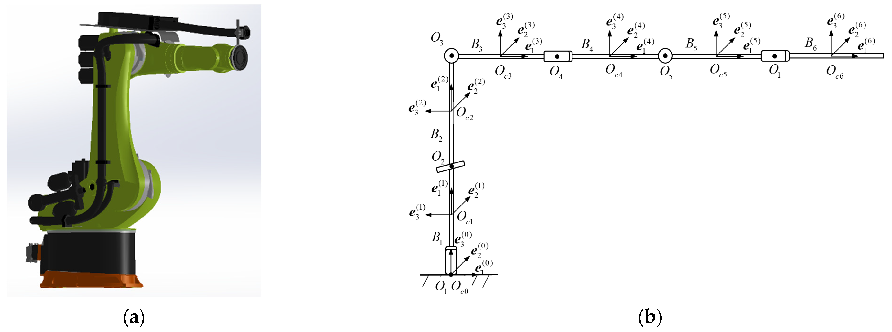
The 6-DOF robot is shown in Figure 1. It consists of 6 rigid bodies $B_i(i=1,2,\cdots ,6)$, of which $B_6$ is the end effector. The robot has 6 rotational DOFs, and the hinge point is $O_i(i=1,2,\cdots ,6)$. Each rigid body is simplified to a homogeneous cylinder of length $l_i$ and radius $R_i$, and the coordinate system $(O_i,{\underset{\_}{\mathit{e}}}^{(i)})(i=1,2,\cdots ,6)$ is established at the position of the centroid $O_{ci}(i=1,2,\cdots ,6)$. The world coordinate system $(O_0,{\underset{\_}{\mathit{e}}}^{(0)})$ is established on the intersection of the centroid of the bottom surface of the base $B_1$ and the ground, and the direction of the base vector ${\mathit{e}}_1^{(i)},{\mathit{e}}_2^{(i)},{\mathit{e}}_3^{(i)}$ of the coordinate system is shown in Figure 1b.

The dynamic equation of a single rigid body $B_i$ is obtained according to Newton–Euler equation:

$$m_i{\ddot{\mathit{r}}}_i={\mathit{F}}_i^g-{\displaystyle \sum _{k=1}^{n_e}{S}_{ik}^{}}{\mathit{F}}_k^{\mathit{e}} (i=1,2,\cdots ,6),$$

(1)

$${\mathit{J}}_i\cdot {\dot{\mathit{\omega }}}_i+{\mathit{\omega }}_i\times ({\mathit{J}}_i\cdot {\mathit{\omega }}_i)=-{\displaystyle \sum _{k=1}^{n_e}({\mathit{C}}_{ik}^{}\times {\mathit{F}}_k^e}+S_{ik}^{}{\mathit{M}}_k^a) (i=1,2,\cdots ,6)$$

(2)

where $m_i$, ${\ddot{\mathit{r}}}_i$, ${\mathit{J}}_i$, ${\mathit{\omega }}_i$, and ${\dot{\mathit{\omega }}}_i$ are the mass, centroid acceleration, principal moment of inertia, angular velocity and angular acceleration of $B_i$, respectively; ${\mathit{F}}_i^g$ is the gravity received by $B_i$, ${\mathit{F}}_k^e$ and ${\mathit{M}}_k^a$ are the force element and active moment exerted on $B_i$ by the inside body $B_{i-1}$, with there being $n_{\mathit{e}}$ in total; the body–hinge vector ${\mathit{C}}_{ik}^{}$ is the vector between the hinge point $O_k(k=i,i+1)$ and the centroid $O_{ci}$, and the directions are all from the inside to the outside, that is, ${\mathit{C}}_{ik}^{}=\frac{1}{2}{l}_i{\mathit{e}}_1^{(i)}(i=1,2,\cdots ,6;k=i,i+1)$; the incidence element $S_{ij}$ is defined as

$$S_{ij}=\{\begin{array}{cc}1& O_j \mathrm{has} \mathrm{incidence} \mathrm{with} B_i \mathrm{and} \mathrm{starts} \mathrm{with} B_i\\ -1& O_j \mathrm{has} \mathrm{incidence} \mathrm{with} B_i \mathrm{and} \mathrm{ends} \mathrm{with} B_i\\ 0& O_j \mathrm{has} \mathrm{no} \mathrm{incidence} \mathrm{with} B_i\end{array}\left(i,j=1,2,\cdots ,n\right).$$

(3)

In order to facilitate computer calculation, the dynamic equations Equations (1) and (2) are written in matrix form (underlined $\underset{\_}{}$ indicates matrix form) as

$$m_i{\underset{\_}{\ddot{\mathit{r}}}}_i={\underset{\_}{\mathit{F}}}_i^g-{\displaystyle \sum _{k=1}^{n_{\mathit{e}}}{S}_{ik}^{}}{\underset{\_}{\mathit{F}}}_k^e (i=1,2,\cdots ,6),$$

(4)

$${\underset{\_}{\mathit{J}}}_i^{(i)}{\underset{\_}{\dot{\mathit{\omega }}}}_i^{(i)}+{\underset{\_}{\tilde{\mathit{\omega }}}}_i^{(i)}{\underset{\_}{\mathit{J}}}_i^{(i)}{\underset{\_}{\mathit{\omega }}}_i^{(i)}=-{\displaystyle \sum _{k=1}^{n_{\mathit{e}}}({\underset{\_}{\mathit{C}}}_{ik}^{}\times {\underset{\_}{\mathit{F}}}_k^e}+S_{ik}^{}{\underset{\_}{\mathit{M}}}_k^a) (i=1,2,\cdots ,6).$$

(5)

The right superscript ${}^{(i)}$ indicates the expression in $(O_i,{\underset{\_}{\mathit{e}}}^{(i)})$, and no superscript indicates the expression in $(O_0,{\underset{\_}{\mathit{e}}}^{(0)})$. ${\underset{\_}{\tilde{\mathit{\omega }}}}_i^{(i)}$ is a third-order antisymmetric matrix:

$${\underset{\_}{\tilde{\mathit{\omega }}}}_i^{(i)}=\left[\begin{array}{ccc}0& -{\mathit{\omega }}_{i3}^{(i)}& {\mathit{\omega }}_{i2}^{(i)}\\ {\mathit{\omega }}_{i3}^{(i)}& 0& -{\mathit{\omega }}_{i1}^{(i)}\\ -{\mathit{\omega }}_{i2}^{(i)}& {\mathit{\omega }}_{i1}^{(i)}& 0\end{array}\right].$$

(6)

${\mathit{\omega }}_{i1}^{(i)},{\mathit{\omega }}_{i2}^{(i)},{\mathit{\omega }}_{i3}^{(i)}$ are the 3 components of ${\underset{\_}{\mathit{\omega }}}_i^{(i)}$ in the ${\mathit{e}}_1^{(i)},{\mathit{e}}_2^{(i)},{\mathit{e}}_3^{(i)}$ directions, respectively.

The angular coordinates of the robot can adopt Euler angles, Cardano angles, Rodrigues parameters and quaternions. However, the first three all have singularities when they move in a wide range of angles, which limits the working space of the robot and makes the robot unable to process large components such as aircraft skins. Quaternions can eliminate singularities and are suitable for motion in a large-angle range, so dynamic parameters can be identified at any pose in the workspace. In addition, for quaternion, there is no need to solve the sine and cosine of the angle coordinates, which reduces the calculation steps and improves the calculation efficiency.

The quaternion is adopted as the generalized angular coordinate, and Euler equation Equation (5) is written as

$$2{\underset{\_}{\mathit{J}}}_i^{(i)}{\underset{\_}{R}}_i^{\ast }{\underset{\_}{\ddot{\Lambda }}}_i+4{\underset{\_}{R}}_i^{\ast }{\underset{\_}{\dot{R}}}_i^{\ast \mathrm{T}}{\underset{\_}{\mathit{J}}}_i^{(i)}{\underset{\_}{R}}_i^{\ast }{\underset{\_}{\dot{\Lambda }}}_i=-{\displaystyle \sum _{k=1}^{n_{\mathit{e}}}({\underset{\_}{\mathit{C}}}_{ik}^{}\times {\underset{\_}{\mathit{F}}}_k^e}+S_{ik}^{}{\underset{\_}{\mathit{M}}}_k^a) (i=1,2,\cdots ,6).$$

(7)

Among these, ${\underset{\_}{\dot{\Lambda }}}_i$ and ${\underset{\_}{\ddot{\Lambda }}}_i$ are the first and second derivatives of the quaternion ${\underset{\_}{\Lambda }}_i={({\lambda }_{i0} {\lambda }_{i1} {\lambda }_{i2} {\lambda }_{i3})}^{\mathrm{T}}$. ${\underset{\_}{R}}_i^{\ast }$ and ${\underset{\_}{\dot{R}}}_i^{\ast \mathrm{T}}$ are as follows:

$${\underset{\_}{R}}_i^{\ast }=\left[\begin{array}{cccc}-{\lambda }_{i1}& {\lambda }_{i0}& {\lambda }_{i3}& -{\lambda }_{i2}\\ -{\lambda }_{i2}& -{\lambda }_{i3}& {\lambda }_{i0}& {\lambda }_{i1}\\ -{\lambda }_{i3}& {\lambda }_{i2}& -{\lambda }_{i1}& {\lambda }_{i0}\end{array}\right] (i=1,2,\cdots ,6),$$

(8)

$${\underset{\_}{\dot{R}}}_i^{\ast \mathrm{T}}=\left[\begin{array}{ccc}-{\dot{\lambda }}_{i1}& -{\dot{\lambda }}_{i2}& -{\dot{\lambda }}_{i3}\\ {\dot{\lambda }}_{i0}& -{\dot{\lambda }}_{i3}& {\dot{\lambda }}_{i2}\\ {\dot{\lambda }}_{i3}& {\dot{\lambda }}_{i0}& -{\dot{\lambda }}_{i1}\\ -{\dot{\lambda }}_{i2}& {\dot{\lambda }}_{i1}& {\dot{\lambda }}_{i0}\end{array}\right] (i=1,2,\cdots ,6).$$

(9)

Since quaternions are not independent parameters, there are self-constraints:

$${\underset{\_}{\Lambda }}_i^{\mathrm{T}}{\underset{\_}{\Lambda }}_i^{}-1=0 (i=1,2,\cdots ,6).$$

(10)

In order to combine with Equation (7), the second derivative of Equation (10) is obtained as

$${\underset{\_}{\Lambda }}_i^{\mathrm{T}}{\underset{\_}{\ddot{\Lambda }}}_i^{}+{\underset{\_}{\dot{\Lambda }}}_i^{\mathrm{T}}{\underset{\_}{\dot{\Lambda }}}_i^{}=0 (i=1,2,\cdots ,6).$$

(11)

Combine Equation (11) with Equation (7), that is, add constraint, and the Euler equation expressed in quaternion coordinates is obtained as

$$\left[\begin{array}{c}2{\underset{\_}{\mathit{J}}}_i^{(i)}{\underset{\_}{R}}_i^{\ast }\\ {\underset{\_}{\Lambda }}_i^{\mathrm{T}}\end{array}\right]{\underset{\_}{\ddot{\Lambda }}}_i^{}+\left[\begin{array}{c}4{\underset{\_}{R}}_i^{\ast }{\underset{\_}{\dot{R}}}_i^{\ast \mathrm{T}}{\underset{\_}{\mathit{J}}}_i^{(i)}{\underset{\_}{R}}_i^{\ast }{\underset{\_}{\dot{\Lambda }}}_i^{}\\ {\underset{\_}{\dot{\Lambda }}}_i^{\mathrm{T}}{\underset{\_}{\dot{\Lambda }}}_i^{}\end{array}\right]=\left[\begin{array}{c}-{\displaystyle \sum _{k=1}^{n_e}({\underset{\_}{\mathit{C}}}_{ik}^{}\times {\underset{\_}{\mathit{F}}}_k^e}+S_{ik}^{}{\underset{\_}{\mathit{M}}}_k^a)\\ 0\end{array}\right] (i=1,2,\cdots ,6).$$

(12)

The combination of Equations (4) and (12) is the dynamic equation of $B_i$ expressed by quaternion, which is abbreviated as

$${\underset{\_}{A}}_i{\underset{\_}{\ddot{q}}}_i={\underset{\_}{B}}_i (i=1,2,\cdots ,6).$$

(13)

where

$$\begin{array}{l}{\underset{\_}{A}}_i=\left[\begin{array}{cc}{m}_i\underset{\_}{E}& \underset{\_}{0}\\ \underset{\_}{0}& 2{\underset{\_}{\mathit{J}}}_i^{(i)}{\underset{\_}{R}}_i^{\ast }\\ \underset{\_}{0}& {\underset{\_}{\Lambda }}_i^{\mathrm{T}}\end{array}\right],{\underset{\_}{B}}_i=\left[\begin{array}{c}\underset{\_}{0}\\ -4{\underset{\_}{R}}_i^{\ast }{\underset{\_}{\dot{R}}}_i^{\ast \mathrm{T}}{\underset{\_}{\mathit{J}}}_i^{(i)}{\underset{\_}{R}}_i^{\ast }\\ -{\underset{\_}{\dot{\Lambda }}}_i^{\mathrm{T}}{\underset{\_}{\dot{\Lambda }}}_i^{}\end{array}\right]+\left[\begin{array}{c}{\underset{\_}{\mathit{F}}}_i^g-{\displaystyle \sum _{k=1}^{n_{\mathit{e}}}{S}_{ik}^{}}{\underset{\_}{\mathit{F}}}_k^e\\ -{\displaystyle \sum _{k=1}^{n_e}({\underset{\_}{\mathit{C}}}_{ik}^{}\times {\underset{\_}{\mathit{F}}}_k^e}+S_{ik}^{}{\underset{\_}{\mathit{M}}}_k^a)\\ 0\end{array}\right]\\ {\underset{\_}{q}}_i={({\underset{\_}{r}}_i {\underset{\_}{\Lambda }}_i)}^{\mathrm{T}}={(x_i y_i z_i {\lambda }_{i0} {\lambda }_{i1} {\lambda }_{i2} {\lambda }_{i3})}^{\mathrm{T}}\end{array}$$

(14)

The dynamic equation of the 6-DOF robot is derived by combining the dynamic equations of the 6 rigid bodies

$$\underset{\_}{A}\underset{\_}{\ddot{q}}=\underset{\_}{B}.$$

(15)

where

$$\underset{\_}{A}=diag({\underset{\_}{A}}_1 \underset{\_}{A}{ }_2 \cdots {\underset{\_}{A}}_6), \underset{\_}{B}={({\underset{\_}{B}}_1^{\mathrm{T}} {\underset{\_}{B}}_2^{\mathrm{T}} \cdots {\underset{\_}{B}}_6^{\mathrm{T}})}^{\mathrm{T}}.$$

(16)

3. Dynamic Parameters Identification of Robot

Dynamic parameters identification is an inverse problem of dynamics. In dynamics, the motion parameters of the robot, that is, the position, velocity and acceleration of rigid bodies, are taken as parameters to be determined. In dynamic parameters identification, the dynamic parameters, that is, the mass and the principal moment of inertia of the rigid bodies, are taken as the parameters to be determined. The two are essentially the same equation, the difference being that the parameters to be identified (output quantities) are different. Therefore, the parameters identification model is obtained by rewriting the dynamic model. The dynamic parameters in the dynamic model are separated as the parameters to be identified. The key lies in decoupling the kinematics and dynamic parameters in the dynamic equation. The multibody dynamic equation can decouple the parameters well and then serve as the theoretical basis for the parameters identification model. In this section, a dynamic parameters identification model is obtained by rewriting the multibody dynamic model, and an identification algorithm is proposed based on the least-squares method. The algorithm can be used to accurately identify the dynamic parameters of the 6-DOF robot.

The dynamic parameters of the robot are the mass $m_i$ and the 3 principal moments of inertia ${\mathit{J}}_{i_{11}}^{(i)},{\mathit{J}}_{i_{22}}^{(i)},{\mathit{J}}_{i_{33}}^{(i)}$ of each rigid body. In order to identify the dynamic parameters of $B_i$, it is necessary to rewrite the Newton–Euler equation into the identification form, that is, to separate $m_i$ and ${\mathit{J}}_{i_{11}}^{(i)},{\mathit{J}}_{i_{22}}^{(i)},{\mathit{J}}_{i_{33}}^{(i)}$ as the parameters to be identified, and use the least-squares method to identify them.

First, Newton equation Equation (4) is rewritten as

$$\left[\begin{array}{ccc}{\ddot{x}}_i& & \\ & {\ddot{y}}_i& \\ & & {\ddot{z}}_i+g\end{array}\right]\left[\begin{array}{c}{m}_i\\ m_i\\ m_i\end{array}\right]=-{\displaystyle \sum _{k=1}^{n_e}{S}_{ik}^{}}{\underset{\_}{\mathit{F}}}_k^e (i=1,2,\cdots ,6).$$

(17)

where ${\ddot{x}}_i,{\ddot{y}}_i,{\ddot{z}}_i$ are the 3 components of ${\ddot{\mathit{r}}}_i$ in the ${\mathit{e}}_1^{(0)},{\mathit{e}}_2^{(0)},{\mathit{e}}_3^{(0)}$ directions, and $g$ is the value of the gravitational acceleration. Equation (17) is the Newton equation in the identification form.

Then, Euler equation Equation (7) is rewritten as

$$\left[\begin{array}{ccc}{}^{id}{S}_{i11}^{(i)}& {}^{id}{S}_{i12}^{(i)}& {}^{id}{S}_{i13}^{(i)}\\ {}^{id}{S}_{i21}^{(i)}& {}^{id}{S}_{i22}^{(i)}& {}^{id}{S}_{i23}^{(i)}\\ {}^{id}{S}_{i31}^{(i)}& {}^{id}{S}_{i32}^{(i)}& {}^{id}{S}_{i33}^{(i)}\end{array}\right]\left[\begin{array}{c}{\mathit{J}}_{i_{11}}^{(i)}\\ {\mathit{J}}_{i_{22}}^{(i)}\\ {\mathit{J}}_{i_{33}}^{(i)}\end{array}\right]=-{\displaystyle \sum _{k=1}^{n_e}({\underset{\_}{\mathit{C}}}_{ik}^{}\times {\underset{\_}{\mathit{F}}}_k^{\mathit{e}}}+S_{ik}^{}{\underset{\_}{\mathit{M}}}_k^a) (i=1,2,\cdots ,6).$$

(18)

where ${\mathit{J}}_{i_{11}}^{(i)},{\mathit{J}}_{i_{22}}^{(i)},{\mathit{J}}_{i_{33}}^{(i)}$ are the 3 components of ${\mathit{J}}_i^{}$ in the ${\mathit{e}}_1^{(i)},{\mathit{e}}_2^{(i)},{\mathit{e}}_3^{(i)}$ directions, and

$$\begin{array}{l}{}^{id}{S}_{i11}^{(i)}=4({\dot{\lambda }}_{i0}{\lambda }_{i0}+{\dot{\lambda }}_{i1}{\lambda }_{i1}+{\dot{\lambda }}_{i2}{\lambda }_{i2}+{\dot{\lambda }}_{i3}{\lambda }_{i3})({\dot{\lambda }}_{i1}{\lambda }_{i0}-{\dot{\lambda }}_{i0}{\lambda }_{i1}+{\dot{\lambda }}_{i2}{\lambda }_{i3}-{\dot{\lambda }}_{i3}{\lambda }_{i2})+2({\ddot{\lambda }}_{i1}{\lambda }_{i0}-{\ddot{\lambda }}_{i0}{\lambda }_{i1}+{\ddot{\lambda }}_{i2}{\lambda }_{i3}-{\ddot{\lambda }}_{i3}{\lambda }_{i2})\\ {}^{id}{S}_{i12}^{(i)}=4({\dot{\lambda }}_{i0}{\lambda }_{i3}-{\dot{\lambda }}_{i1}{\lambda }_{i2}+{\dot{\lambda }}_{i2}{\lambda }_{i1}-{\dot{\lambda }}_{i3}{\lambda }_{i0})({\dot{\lambda }}_{i2}{\lambda }_{i0}-{\dot{\lambda }}_{i0}{\lambda }_{i2}-{\dot{\lambda }}_{i1}{\lambda }_{i3}+{\dot{\lambda }}_{i3}{\lambda }_{i1})\\ {}^{id}{S}_{i13}^{(i)}=4({\dot{\lambda }}_{i2}{\lambda }_{i0}-{\dot{\lambda }}_{i0}{\lambda }_{i2}-{\dot{\lambda }}_{i1}{\lambda }_{i3}+{\dot{\lambda }}_{i3}{\lambda }_{i1})({\dot{\lambda }}_{i1}{\lambda }_{i2}-{\dot{\lambda }}_{i0}{\lambda }_{i3}-{\dot{\lambda }}_{i2}{\lambda }_{i1}+{\dot{\lambda }}_{i3}{\lambda }_{i0})\\ {}^{id}{S}_{i21}^{(i)}=4({\dot{\lambda }}_{i1}{\lambda }_{i2}-{\dot{\lambda }}_{i0}{\lambda }_{i3}-{\dot{\lambda }}_{i2}{\lambda }_{i1}+{\dot{\lambda }}_{i3}{\lambda }_{i0})({\dot{\lambda }}_{i1}{\lambda }_{i0}-{\dot{\lambda }}_{i0}{\lambda }_{i1}+{\dot{\lambda }}_{i2}{\lambda }_{i3}-{\dot{\lambda }}_{i3}{\lambda }_{i2})\\ {}^{id}{S}_{i22}^{(i)}=4({\dot{\lambda }}_{i0}{\lambda }_{i0}+{\dot{\lambda }}_{i1}{\lambda }_{i1}+{\dot{\lambda }}_{i2}{\lambda }_{i2}+{\dot{\lambda }}_{i3}{\lambda }_{i3})({\dot{\lambda }}_{i2}{\lambda }_{i0}-{\dot{\lambda }}_{i0}{\lambda }_{i2}-{\dot{\lambda }}_{i1}{\lambda }_{i3}+{\dot{\lambda }}_{i3}{\lambda }_{i1})+2({\ddot{\lambda }}_{i2}{\lambda }_{i0}-{\ddot{\lambda }}_{i0}{\lambda }_{i2}-{\ddot{\lambda }}_{i1}{\lambda }_{i3}+{\ddot{\lambda }}_{i3}{\lambda }_{i1})\\ {}^{id}{S}_{i23}^{(i)}=4({\dot{\lambda }}_{i0}{\lambda }_{i1}-{\dot{\lambda }}_{i1}{\lambda }_{i0}-{\dot{\lambda }}_{i2}{\lambda }_{i3}+{\dot{\lambda }}_{i3}{\lambda }_{i2})({\dot{\lambda }}_{i1}{\lambda }_{i2}-{\dot{\lambda }}_{i0}{\lambda }_{i3}-{\dot{\lambda }}_{i2}{\lambda }_{i1}+{\dot{\lambda }}_{i3}{\lambda }_{i0})\\ {}^{id}{S}_{i31}^{(i)}=4({\dot{\lambda }}_{i0}{\lambda }_{i2}-{\dot{\lambda }}_{i2}{\lambda }_{i0}+{\dot{\lambda }}_{i1}{\lambda }_{i3}-{\dot{\lambda }}_{i3}{\lambda }_{i1})({\dot{\lambda }}_{i1}{\lambda }_{i0}-{\dot{\lambda }}_{i0}{\lambda }_{i1}+{\dot{\lambda }}_{i2}{\lambda }_{i3}-{\dot{\lambda }}_{i3}{\lambda }_{i2})\\ {}^{id}{S}_{i32}^{(i)}=4({\dot{\lambda }}_{i1}{\lambda }_{i0}-{\dot{\lambda }}_{i0}{\lambda }_{i1}+{\dot{\lambda }}_{i2}{\lambda }_{i3}-{\dot{\lambda }}_{i3}{\lambda }_{i2})({\dot{\lambda }}_{i2}{\lambda }_{i0}-{\dot{\lambda }}_{i0}{\lambda }_{i2}-{\dot{\lambda }}_{i1}{\lambda }_{i3}+{\dot{\lambda }}_{i3}{\lambda }_{i1})\\ {}^{id}{S}_{i33}^{(i)}=4({\dot{\lambda }}_{i0}{\lambda }_{i0}+{\dot{\lambda }}_{i1}{\lambda }_{i1}+{\dot{\lambda }}_{i2}{\lambda }_{i2}+{\dot{\lambda }}_{i3}{\lambda }_{i3})({\dot{\lambda }}_{i1}{\lambda }_{i2}-{\dot{\lambda }}_{i0}{\lambda }_{i3}-{\dot{\lambda }}_{i2}{\lambda }_{i1}+{\dot{\lambda }}_{i3}{\lambda }_{i0})+2({\ddot{\lambda }}_{i1}{\lambda }_{i2}-{\ddot{\lambda }}_{i0}{\lambda }_{i3}-{\ddot{\lambda }}_{i2}{\lambda }_{i1}+{\ddot{\lambda }}_{i3}{\lambda }_{i0})\end{array}$$

(19)

Since the quaternions are not independent parameters, constraints need to be added, so the quaternion self-constraint condition Equation (10) is combined with Equation (18) as

$$\left[\begin{array}{cc}\begin{array}{ccc}{}^{id}{S}_{i11}^{(i)}& {}^{id}{S}_{i12}^{(i)}& {}^{id}{S}_{i13}^{(i)}\\ {}^{id}{S}_{i21}^{(i)}& {}^{id}{S}_{i22}^{(i)}& {}^{id}{S}_{i23}^{(i)}\\ {}^{id}{S}_{i31}^{(i)}& {}^{id}{S}_{i32}^{(i)}& {}^{id}{S}_{i33}^{(i)}\end{array}& \\ & {\underset{\_}{\Lambda }}_i^{\mathrm{T}}{\underset{\_}{\Lambda }}_i^{}-1\end{array}\right]\left[\begin{array}{c}{}^{id}{\underset{\_}{\mathit{J}}}_i^{(i)}\\ 1\end{array}\right]=\left[\begin{array}{c}-{\displaystyle \sum _{k=1}^{n_e}({\underset{\_}{\mathit{C}}}_{ik}^{}\times {\underset{\_}{\mathit{F}}}_k^e}+S_{ik}^{}{\underset{\_}{\mathit{M}}}_k^a)\\ 0\end{array}\right] (i=1,2,\cdots ,6).$$

(20)

Equation (20) is the Euler equation in the identification form.

Finally, by combining Equations (17) and (20), the dynamic equation in the identification form of $B_i$ is obtained, which is abbreviated as

$${}^{id}\underset{\_}{Y}_i{}^{id}\underset{\_}{X}_i={}^{id}\underset{\_}{Z}_i.$$

(21)

where

$${}^{id}\underset{\_}{Y}_i=\left[\begin{array}{ccccc}{\ddot{x}}_i& & & & \\ & {\ddot{y}}_i& & & \\ & & {\ddot{z}}_i+g& & \\ & & & \begin{array}{cc}\begin{array}{ccc}{}^{id}{S}_{i11}^{(i)}& {}^{id}{S}_{i12}^{(i)}& {}^{id}{S}_{i13}^{(i)}\\ {}^{id}{S}_{i21}^{(i)}& {}^{id}{S}_{i22}^{(i)}& {}^{id}{S}_{i23}^{(i)}\\ {}^{id}{S}_{i31}^{(i)}& {}^{id}{S}_{i32}^{(i)}& {}^{id}{S}_{i33}^{(i)}\end{array}& \\ \end{array}& \\ & & & & {\underset{\_}{\Lambda }}_i^{\mathrm{T}}{\underset{\_}{\Lambda }}_i^{}-1\end{array}\right],{}^{id}{\underset{\_}{X}}_i=\left[\begin{array}{c}{}^{id}{\underset{\_}{m}}_i\\ \begin{array}{c}{}^{id}{\underset{\_}{\mathit{J}}}_i^{(i)}\\ 1\end{array}\end{array}\right],{}^{id}{\underset{\_}{Z}}_i=\left[\begin{array}{c}-{\displaystyle \sum _{k=1}^{n_e}{S}_{ik}^{}}{\underset{\_}{\mathit{F}}}_k^e\\ \begin{array}{c}-{\displaystyle \sum _{k=1}^{n_e}({\underset{\_}{\mathit{C}}}_{ik}^{}\times {\underset{\_}{\mathit{F}}}_k^e}+S_{ik}^{}{\underset{\_}{\mathit{M}}}_k^a)\\ 0\end{array}\end{array}\right].$$

(22)

In order to improve the reliability and accuracy of the parameter ${}^{id}{\underset{\_}{X}}_i$ to be identified, it is necessary to sample ${}^{id}{\underset{\_}{Y}}_i{,}^{id}{\underset{\_}{Z}}_i$ at multiple times and obtain multiple sets of data.

For time $t_j$,

$${}_j^{id}{\underset{\_}{Y}}_i={}^{id}{\underset{\_}{X}}_i{}_j^{id}{\underset{\_}{Z}}_i.$$

(23)

where ${}_j^{id}{\underset{\_}{Y}}_i{,}_j^{id}{\underset{\_}{Z}}_i$ is the sampled data at time $t_j$.

Sampling occurred $n$ times, namely $1\le j\le n$, corresponding to $t_j(j=1,2,\cdots ,n)$, respectively. (It should be noted that the selection of these $n$ times is arbitrary. $n$ times in the motion process can be randomly selected, and the accuracy of the identification results will not be affected by the selection of sampling times.) Then, the equation system is composed, abbreviated as

$${}^{id}{\underset{\_}{K}}_i{}^{id}{\underset{\_}{X}}_i={}^{id}{\underset{\_}{L}}_i.$$

(24)

where

$${}^{id}{\underset{\_}{K}}_i=\left[\begin{array}{c}{}_1^{id}{\underset{\_}{Y}}_i\\ {}_2^{id}{\underset{\_}{Y}}_i\\ ⋮\\ {}_n^{id}{\underset{\_}{Y}}_i\end{array}\right],{}^{id}{\underset{\_}{L}}_i=\left[\begin{array}{c}{}_1^{id}{\underset{\_}{Z}}_i\\ {}_2^{id}{\underset{\_}{Z}}_i\\ ⋮\\ {}_n^{id}{\underset{\_}{Z}}_i\end{array}\right].$$

(25)

Equation (24) is the dynamic equation in the identification form of $B_i$ after sampling $n$ times, and its least-squares solution is

$${}^{id}{\underset{\_}{X}}_i={({{}^{id}{\underset{\_}{K}}_i}^{\mathrm{T}}{}^{id}{\underset{\_}{K}}_i)}^{-1}{{}^{id}{\underset{\_}{K}}_i}^{\mathrm{T}}{}^{id}{\underset{\_}{L}}_i.$$

(26)

The dynamic parameters of $B_i$ can be identified according to Equation (26).

The dynamic equation in identification form of the 6-DOF robot is obtained by combining the dynamic equations in identification form of the 6 rigid bodies:

$${}^{id}\underset{\_}{X}={({{}^{id}\underset{\_}{K}}^{\mathrm{T}}{}^{id}\underset{\_}{K})}^{-1}{{}^{id}\underset{\_}{K}}^{\mathrm{T}}{}^{id}\underset{\_}{L}.$$

(27)

where

$${}^{id}\underset{\_}{X}=\left[\begin{array}{c}{}_{}^{id}{\underset{\_}{X}}_1\\ {}_{}^{id}{\underset{\_}{X}}_2\\ ⋮\\ {}_{}^{id}{\underset{\_}{X}}_6\end{array}\right],{}^{id}\underset{\_}{K}=\left[\begin{array}{c}{}_{}^{id}{\underset{\_}{K}}_1\\ {}_{}^{id}{\underset{\_}{K}}_2\\ ⋮\\ {}_{}^{id}{\underset{\_}{K}}_6\end{array}\right],{}^{id}\underset{\_}{L}=\left[\begin{array}{c}{}_{}^{id}{\underset{\_}{L}}_1\\ {}_{}^{id}{\underset{\_}{L}}_2\\ ⋮\\ {}_{}^{id}{\underset{\_}{L}}_6\end{array}\right].$$

(28)

4. Numerical Simulation Example

The three-dimensional model of the robot is established with ADAMS software, and numerical simulation is carried out to verify the correctness and accuracy of the identification algorithm.

Each rigid body is regarded as a homogeneous cylinder, the material is steel, and the gravity acceleration value is set to 9.80665. The length $l_i$ and radius $R_i$ of each $B_i$ are set to obtain the true values of dynamic parameters, as shown in

Table 1. Physical parameters of each rigid body.

$\mathbf{Rigid} \mathbf{Body} {\mathit{B}}_{\mathit{i}}$	${\mathit{B}}_1$	${\mathit{B}}_2$	${\mathit{B}}_3$	${\mathit{B}}_4$	${\mathit{B}}_5$	${\mathit{B}}_6$
$l_i$ (m)	1.045	1.245	1.21	0.315	0.29	0.3
$R_i$ (m)	0.5	0.3	0.2	0.2	0.2	0.3
$m_i$ (kg)	6402.6012	2746.0726	1186.1661	308.7953	284.2877	661.7042
${\mathit{J}}_{i_{11}}^{(i)}$ (kg·m2)	800.3251	123.5733	23.7233	6.1759	5.6858	29.7767
${\mathit{J}}_{i_{22}}^{(i)}$ (kg·m2)	982.8126	416.4934	156.5838	5.6413	4.8353	19.8511
${\mathit{J}}_{i_{33}}^{(i)}$ (kg·m2)	982.8126	416.4934	156.5838	5.6413	4.8353	19.8511

.

Movement target: The robot only moves once, so that the generated data can identify the dynamic parameters of the six rigid bodies of the robot at the same time.

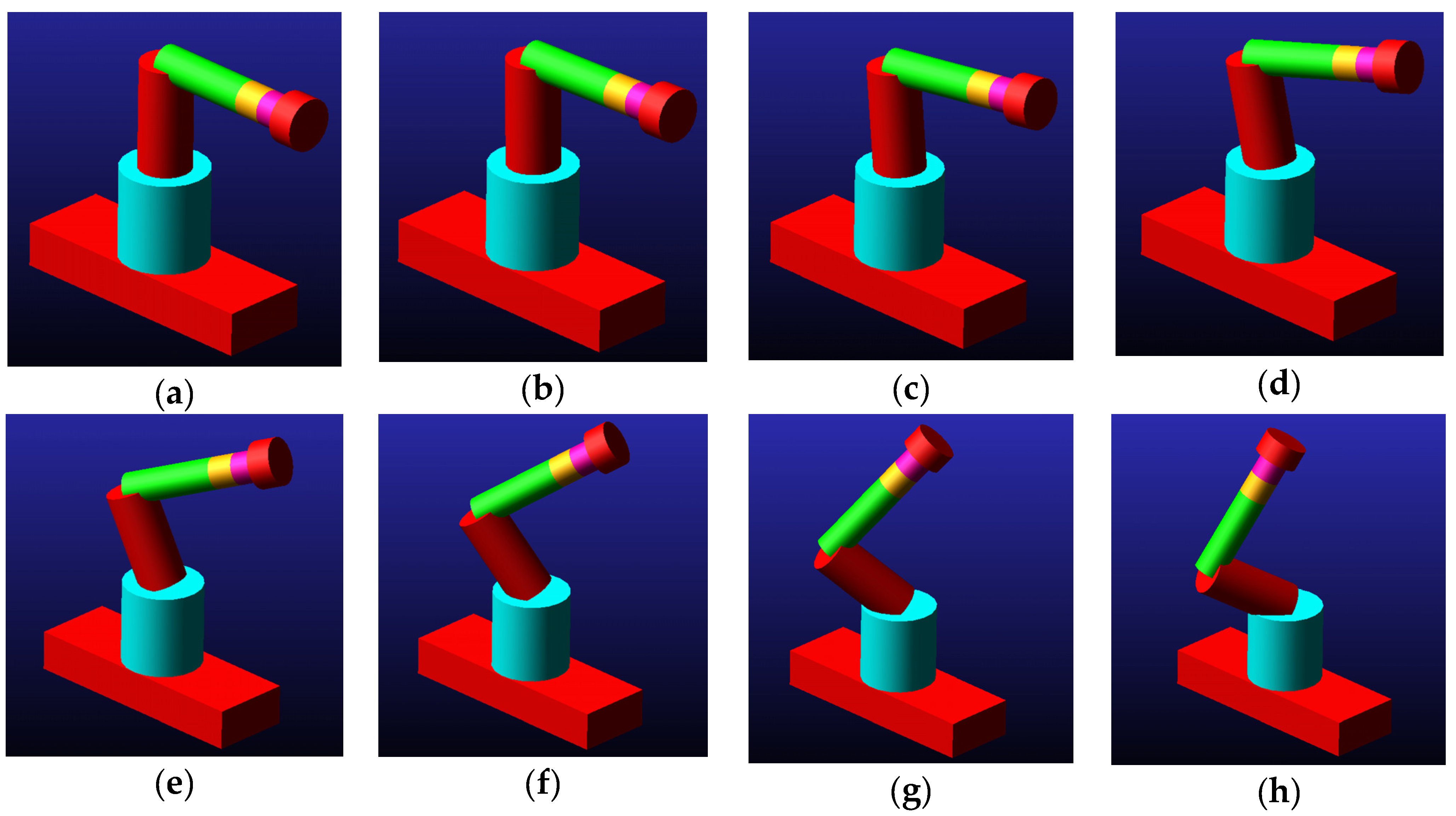
Movement settings: the initial state is still, and the posture is shown in Figure 1. Both hinge $O_1$ and hinge $O_2$ rotate at the angular acceleration of 9.5493 rad/s² (that is, 30°/s²), and all other hinges are locked so that they do not rotate. The simulation termination time is 2 s, and the number of steps is 100. The pose change of the robot during the movement is shown in Figure 2.

Theoretically, the number of the groups of selected data and the accuracy of the identification result are positively correlated. However, larger data volume may lead to an increase in the complexity of and time consuming by the calculation. In this experiment, five groups of data are selected, which are the data for 0.3 s, 0.6 s, 0.9 s, 1.2 s and 1.5 s (other arbitrary times can also be randomly selected).

The types of sampled data are as follows. We sampled the quaternion coordinates, as well as the force element ${\mathit{F}}_i^e$ and acting moment ${\mathit{M}}_i^a$, of the inside body. Additionally, the angular velocity, angular acceleration and centroid acceleration of each rigid body are also sampled.

The dynamic parameters are identified by Equation (27), and the results are shown in

Table 2. Identified dynamic parameters of robot.

$\mathbf{Rigid} \mathbf{Body} {\mathit{B}}_{\mathit{i}}$	${\mathit{B}}_1$	${\mathit{B}}_2$	${\mathit{B}}_3$	${\mathit{B}}_4$	${\mathit{B}}_5$	${\mathit{B}}_6$
$m_i$$({\mathit{e}}_1^{(0)}$) (kg)	—	2746.0722	1186.1661	308.7955	284.2877	661.7043
$m_i$$({\mathit{e}}_2^{(0)}$) (kg)	—	2746.0723	1186.1661	308.7955	284.2875	661.7043
$m_i$$({\mathit{e}}_3^{(0)}$) (kg)	6402.6044	2746.0723	1186.1660	308.7955	284.2877	661.7042
${\mathit{J}}_{i_{11}}^{(i)}$ (kg·m2)	800.3250	123.5954	23.7230	6.1756	5.6862	29.7768
${\mathit{J}}_{i_{22}}^{(i)}$ (kg·m2)	982.8128	416.4670	156.5862	5.6405	4.8355	19.8512
${\mathit{J}}_{i_{33}}^{(i)}$ (kg·m2)	982.8128	416.4991	156.5844	5.6404	4.8368	19.8514

.

Among these, $m_i$(${\mathit{e}}_1^{(0)}$), $m_i$(${\mathit{e}}_2^{(0)}$), $m_i$(${\mathit{e}}_3^{(0)}$) are the identified mass parameters of $B_i$ in the ${\mathit{e}}_1^{(0)}$, ${\mathit{e}}_2^{(0)}$, ${\mathit{e}}_3^{(0)}$ directions, respectively. In particular, since $B_1$ only has acceleration in the ${\mathit{e}}_3^{(0)}$ direction, the mass parameters in the ${\mathit{e}}_1^{(0)},{\mathit{e}}_2^{(0)}$ directions cannot be identified.

The accuracy of the identification algorithm can be quantitatively evaluated by the absolute error between the identified dynamic parameters and their true values. The absolute error is shown in

Table 3. The absolute error between the dynamic parameters and their real values.

Rigid Body	Absolute Error
	${\mathit{m}}_{\mathit{i}}$$({\mathit{e}}_1^{(0)}$) $\left(\mathbf{k}\mathbf{g}\right)$	${\mathit{m}}_{\mathit{i}}$$({\mathit{e}}_2^{(0)}$) $\left(\mathbf{k}\mathbf{g}\right)$	${\mathit{m}}_{\mathit{i}}$$({\mathit{e}}_3^{(0)}$) $\left(\mathbf{k}\mathbf{g}\right)$	${\mathit{J}}_{{\mathit{i}}_{11}}^{(\mathit{i})}$ $(\mathbf{k}\mathbf{g}\cdot {\mathbf{m}}^2)$	${\mathit{J}}_{{\mathit{i}}_{22}}^{(\mathit{i})}$ $(\mathbf{k}\mathbf{g}\cdot {\mathbf{m}}^2)$	${\mathit{J}}_{{\mathit{i}}_{33}}^{(\mathit{i})}$ $(\mathbf{k}\mathbf{g}\cdot {\mathbf{m}}^2)$
$B_6$	0.0001	0.0001	0	0.0001	0.0001	0.0003
$B_5$	0	−0.0002	0	0.0004	0.0002	0.0015
$B_4$	0.0002	0.0002	0.0002	−0.0003	−0.0008	−0.0009
$B_3$	0	0	−0.0001	−0.0003	0.0024	0.0006
$B_2$	−0.0004	−0.0003	−0.0003	0.0224	−0.0264	0.0057
$B_1$	—	—	0.0032	−0.0001	0.0002	0.0002

.

An analysis of the causes of the absolute error is as follows. First, the identification algorithm based on the dynamic model involves many variables and requires a large number of calculations, and the calculation results can only retain a limited number of significant figures. Therefore, the operation times of the computation and the accumulated absolute error are positively correlated. Second, the counting rule of the ADAMS software is that the data retain 7 significant figures, so the value of the data is positively correlated with the absolute error, and the number of decimal places reserved for the data is negatively correlated with the absolute error.

According to Table 3, the value of the maximum absolute error of the identified dynamic parameters is as low as −0.0264, and according to the absolute errors, the maximum relative error can be obtained as 0.031%, which verifies the correctness and accuracy of the identification algorithm.

The previous parameters identification research aimed to identify the velocity, acceleration, joint torque or nonlinear coupling terms of dynamic parameters, which cannot identify the dynamic parameters directly. Moreover, the research is based on models with different degrees of simplification, and the relative errors of the identified parameters are usually in the range of several percentage points. The previous research is indeed very meaningful for solving practical problems encountered by researchers, and it must be affirmed. However, this method does not apply to our research, and we need to develop a new method.

A more complex and accurate identification algorithm is proposed for the first time in this paper. Compared with previous studies, the algorithm is different as follows. First, the models are different. The identification algorithm in this paper is based on a multibody dynamic model, and the model is not simplified, so it is more accurate. Although an accurate model leads to a more complex derivation process and more data sampling, it is very necessary to improve the accuracy of identification. Second, the identified parameters are different. The dynamic parameters (rather than the nonlinear coupling term of the dynamic parameters) can be decoupled and directly used as the dynamic parameters to be identified in the identification algorithm of this paper. The nonlinear coupling term of dynamic parameters is only applicable to a specific identification model and is not universal. Different models have different nonlinear coupling terms to be identified; dynamic parameters are applicable to all models and are more universal. Third, the accuracy is improved. Because the model is more accurate and the dynamic parameters are decoupled, the algorithm can identify the dynamic parameters more accurately, and the relative errors of the identified parameters are all less than 0.031%. Since the error is limited to a small range, the identification accuracy of this algorithm can meet the requirement of precise control.

5. Conclusions

In this paper, the problem of dynamic parameters identification is studied, and an identification algorithm is proposed, which can be used to accurately identify the dynamic parameters of the 6-DOF industrial robot.

(1)

The identification algorithm is based on the multibody dynamic model. The kinematic and dynamic parameters of each rigid body of the robot can be decoupled in the multibody dynamic model. Since parameters decoupling is the basis of the identification algorithm, the multibody dynamic model is especially suitable for multi-DOF robots.

(2)

The quaternions are used as angular coordinates in the identification algorithm, which eliminates the singularity and makes the algorithm suitable for the large-angle range of motion; at the same time, the calculation efficiency is improved, which enables the algorithm to have better real-time performance.

(3)

Numerical simulation of the identification algorithm is carried out. The results show that the value of the maximum absolute error of the identified parameters is −0.0264, and the maximum relative error is 0.031%. The algorithm is correct and accurate, which provides a theoretical basis for the accurate identification of dynamic parameters and has positive significance for the precise control and vibration reduction of the robot.

References

- Liu, W.; Huo, X.; Liu, J.; Wang, L. Parameter identification for a quadrotor helicopter using multivariable extremum seeking algorithm. Int. J. Control Autom. Syst. 2018, 16, 1951–1961. [Google Scholar] [CrossRef]
- Urrea, C.; Saa, D. Design and implementation of a graphic simulator for calculating the inverse kinematics of a redundant planar manipulator robot. Appl. Sci. 2020, 10, 6770. [Google Scholar] [CrossRef]
- Armstrong, B.; Khatib, O.; Burdick, J. The explicit dynamic model and inertial parameters of the PUMA 560 arm. In Proceedings of the 1986 IEEE International Conference on Robotics and Automation, San Francisco, CA, USA, 7–10 April 1986; IEEE: Piscataway, NJ, USA, 1986; Volume 3, pp. 510–518. [Google Scholar]
- Zhou, Y.; Luo, J.; Wang, M. Dynamic coupling analysis of multi-arm space robot. Acta Astronaut. 2019, 160, 583–593. [Google Scholar] [CrossRef]
- Khalil, W.; Dombre, E. Modeling Identification and Control of Robots; CRC Press: Boca Raton, FL, USA, 2002. [Google Scholar]
- Olsen, M.M.; Swevers, J.; Verdonck, W. Maximum likelihood identification of a dynamic robot model: Implementation issues. Int. J. Robot. Res. 2002, 21, 89–96. [Google Scholar] [CrossRef]
- Gautier, M.; Janot, A.; Vandanjon, P.O. A new closed-loop output error method for parameter identification of robot dynamics. IEEE Trans. Control Syst. Technol. 2012, 21, 428–444. [Google Scholar] [CrossRef] [Green Version]
- Wang, S.; Shao, X.; Yang, L.; Liu, N. Deep learning aided dynamic parameter identification of 6-DOF robot manipulators. IEEE Access 2020, 8, 138102–138116. [Google Scholar] [CrossRef]
- Xu, T.; Fan, J.; Chen, Y.; Ng, X.; Ang, M.H.; Fang, Q.; Zhu, Y.; Zhao, J. Dynamic identification of the KUKA LBR iiwa robot with retrieval of physical parameters using global optimization. IEEE Access 2020, 8, 108018–108031. [Google Scholar] [CrossRef]
- Urrea, C.; Pascal, J. Dynamic Parameter Identification Based on Lagrangian Formulation and Servomotor-type Actuators for Industrial Robots. Int. J. Control Autom. Syst. 2021, 19, 2902–2909. [Google Scholar] [CrossRef]
- Díaz-Rodríguez, M.; Mata, V.; Valera, A.; Page, A. A methodology for dynamic parameters identification of 3-DOF parallel robots in terms of relevant parameters. Mech. Mach. Theory 2010, 45, 1337–1356. [Google Scholar] [CrossRef]
- Gaz, C.; Cognetti, M.; Oliva, A.; Giordano, P.R.; De Luca, A. Dynamic identification of the franka emika panda robot with retrieval of feasible parameters using penalty-based optimization. IEEE Robot. Autom. Lett. 2019, 4, 4147–4154. [Google Scholar] [CrossRef] [Green Version]
- Briot, S.; Gautier, M. Global identification of joint drive gains and dynamic parameters of parallel robots. Multibody Syst. Dyn. 2015, 33, 3–26. [Google Scholar] [CrossRef] [Green Version]
- Hardeman, T.; Aarts, R.G.; Jonker, J.B. A finite element formulation for dynamic parameter identification of robot manipulators. Multibody Syst. Dyn. 2006, 16, 21–35. [Google Scholar] [CrossRef]
Figure 1.
The 6-DOF robot and schematic diagram of its coordinate system. (a) 6-DOF robot; (b) Schematic diagram of coordinate system of 6-DOF robot.
Figure 2.
The poses at each time in the ADAMS simulation of the 6-DOF robot. (a) 0 s; (b) 0.3 s; (c) 0.6 s; (d) 0.9 s; (e) 1.2 s; (f) 1.5 s; (g) 1.8 s; (h) 2 s.