Geometric Algebra Applied to Multiphase Electrical Circuits in Mixed Time–Frequency Domain by Means of Hypercomplex Hilbert Transform

Abstract

In this paper, power flows in electrical circuits are modelled in a mixed time-frequency domain by using geometric algebra and the Hilbert transform for the first time. The use of this mathematical framework overcomes some of the limitations of some of the existing methodologies, in which the so-called “active current” may not lead to the lowest Root Mean Square (RMS) current under distorted supply or unbalanced load. Moreover, this current may contain higher levels of harmonic distortion compared to the supply voltage. The proposed method can be used for sinusoidal and non-sinusoidal power supplies, non-linear loads and single- and multi-phase electrical circuits, and it provides meaningful engineering results with a compact formulation. It can also serve as an advanced tool for developing algorithms in the power electronics field. Several examples have been included to verify the validity of the proposed theory.

1. Introduction

Pioneer power theories and circuit analysis for electrical circuits were developed by the end of the XIX century. Renowned engineers and scientists such as Steinmetz, Kennelly and Heaviside (among others) made great contributions in this field [1,2,3]. Currently, these theories are still a source of discussion and debate concerning their correctness and physical interpretation [4,5,6,7]. Some of these theories were formulated in the frequency domain, such as those proposed by Budeanu [8] and Czarnecki [9], while others were formulated in the time domain, such as those presented by Fryze [10], Akagi [11] and Depenbrock [12,13]. Many other approaches have also been formulated recently [14,15]. In the same vein, Lev-Ari [16], Salmerón [17] and Ustariz [18,19] have made relevant contributions to the field by using the Hilbert Transform (HT) and tensor algebra, respectively. All these theories are devoted to explaining the power-transfer process between complex electrical systems and they establish mathematical concepts associated with fictitious powers (e.g., non-active power), which are of a great interest from a mathematical and engineering point of view [20,21]. Unfortunately, none of the existing proposals can be used to separate current components in the time domain under arbitrary types of voltage harmonic distortion, asymmetry, non-linearity of the load or combinations thereof. This fact has been reported several times in the literature [4,22]. For example, a source voltage containing unbalanced and non-sinusoidal voltage components is a typical case where theories such as Instantaneous Reactive Power (IRP) produce inadequate results [23,24].

In this paper, a new proposal is presented to overcome the aforementioned limitations by applying two mathematical tools: Geometric Algebra (GA) [25,26] and Hilbert Transform (HT). GA is a versatile tool that can be used to model different physical and mathematical problems [27,28]. The application of GA makes it possible to separate current components that have engineering relevance for circuits with any number of phases (including single-phase circuits) [29,30]. The term “engineering relevance” is explicitly used while the term “physical relevance” is avoided, mainly because one of the main applications of power theories is current decomposition for load compensation purposes. Indeed, there is still controversy regarding the physical meaning of these current components [31]. However, it is clear that they are relevant for engineering practice. Current decomposition is addressed by using both instantaneous and average currents so that currents that do not contribute to active power can be compensated. This paper is not intended to reveal the physical meaning of power terms (see [32] for details). In fact, it is well known that this is a challenging task where the Poynting vector should be involved. On the other hand, thanks to the use of the HT [33,34], the proposed theory can also be applied to single-phase systems seamlessly, which is a relevant advantage compared to the existing theories. A variety of applications could benefit from the techniques presented in this paper. In particular, it can be easier to understand current components in active power filters working under distorted grid conditions [35]. Additionally, they may be applied to multi-phase AC machinery, where in-depth knowledge of voltage and current waveforms is critical to improve their performance [36]. Other applications in which waveforms are prone to be distorted (such as reactive-power compensation [37], microgrids [38] and power electronics converter control [39]) are target applications.

The paper includes an overview of GA in order to make the paper self-contained. However, for detailed information about GA and its applications to electrical circuits, see references [26,40]. A historical perspective can also be found in Chappell [41]. The developments presented in this paper are mainly fundamental and are explained with simple examples so that the basics of the theory can be easily understood. The application of this theory to large power systems is also of interest. This would require research efforts and it is considered of interest for further research.

Contributions

The contributions and novelties of this paper are summarised below. The remainder of this section elaborates on these points:

• A general framework based on GA is proposed and applied to electrical circuits in a mixed time–frequency domain.
  This makes it possible to handle the voltages, currents and powers in single and multiple phases. The geometric power is defined based on these concepts.
• Based on the concept of monogenic signals, we apply the hypercomplex HT to construct multi-dimensional analytic signals in the field of electric circuits, for the first time.
• The instantaneous geometric impedance is presented as an alternative method to characterise loads in the time domain.

The first contribution of this paper is to provide an alternative and unified approach to describe the power flow in mixed time–frequency domain in terms of GA. Previous works on this field have applied a large number of mathematical tools such as complex numbers, quaternions, vectors, matrices, tensors, differential forms, etc. All these techniques can be considered subspaces of a general geometric space that can be named ${\mathcal{G}}^n$. Due to the aforementioned reasons, GA has been described in the literature as a unifying tool [42,43].

The second contribution is to present a new way to build multi-dimensional signals by using the HT, which are also known as monogenic signals in the context of Clifford algebras [44]. This is the first application of this technique to electrical circuits, to the best of the authors’ knowledge. The proposed method allows using voltage and current vectors that preserve orthogonality. As a consequence, the geometric power can be defined, which has clear engineering relevance (e.g., in active power filtering applications). In this regard, the application of the IRP theory has led to controversial results. For example, Haley [22] demonstrated that the application of a purely symmetrical voltage to an unbalanced load (composed of a resistor between the phase R and the neutral) produces a compensation current that contains third-order harmonic and negative sequence components. However, the application of the theory proposed in this paper leads to a result with a more clear physical meaning (a compensation current that is symmetrical and balanced), which also minimises the RMS value of the current. Other studies have also highlighted similar flaws [24]. Moreover, the use of the multi-analytic signal also allows computation of single and multi-phase currents and voltages. These features are not available on other power theories, simultaneously. It allows study of the bidirectionality of the distributed energy resources in heterogeneous power grids and their impact on system losses from an optimal point of view irrespective of the properties of the power source and the load.

The third contribution is related to the definition of an instantaneous impedance in geometric terms. By linking the so-called in-band components, the load can be characterised in the time domain. This feature can be exploited for the characterisation of loads consisting of several components (e.g., power electronics converters with their control loops, rectifiers, etc.)

2. Geometric Algebra and Power Theory

2.1. Hilbert Transform and Geometric Algebra Fundamentals

The HT ($\mathcal{H}$) is defined in the time domain as the convolution of the Hilbert transformer $1/\pi t$ and a function $f\left(t\right)$:

$$\mathcal{H}\left[f\left(t\right)\right]=\frac{1}{\pi }PV{\int }_{-\infty }^{+\infty }\frac{f\left(\tau \right)}{\tau -t}d\tau$$

(1)

where $PV$ is the Cauchy principal value to handle the singularity at $t=\tau$. The Bracewell criteria are used to select the sign of the transformation [45]. The HT is revealed to be a crucial tool to calculate quadrature signals [16] and will be used to compute a sort of (geometric) impedance in the time domain. It is also used in other areas related to empirical mode decomposition and machine learning [46]. It can be proved that the HT delays positive frequency components (fundamental and harmonics) by $\pi /2$ [33]. Note that the use of the HT automatically implies that averaged quantities are used, i.e., at least one period of the signal needs to be analysed. In general, $\parallel \mathcal{H}\left[f\left(t\right)\right]\parallel \ne \parallel f\left(t\right)\parallel$ due to the presence of a DC component [47]. The use of the HT for voltages and currents in electrical circuits to obtain transformed analytic functions in the complex domain is well known [48]. As an example, consider

$$\begin{array}{cc}\hfill \overline{u}\left(t\right)& =u\left(t\right)+j\mathcal{H}\left[u\left(t\right)\right]\hfill \\ \hfill \overline{i}\left(t\right)& =i\left(t\right)+j\mathcal{H}\left[i\left(t\right)\right]\hfill \end{array}$$

(2)

where the decoration bar means a complex quantity, $u\left(t\right)$ and $i\left(t\right)$ are arbitrary voltage and current signals and j is the imaginary unit.

Consider now an orthonormal basis $\mathbf{\sigma }=\{{\mathbf{\sigma }}_1,{\mathbf{\sigma }}_2,\dots ,{\mathbf{\sigma }}_n\}$ defined for a Euclidean vector space in ${\mathcal{R}}^n$. Then, it is possible to establish a new geometric vector space ${\mathcal{G}}^n$ with a bilinear operation. Under these assumptions, a vector can be represented as:

$$\mathit{a}=\sum _n{a}_n{\mathbf{\sigma }}_n=a_1{\mathbf{\sigma }}_1+\dots +a_n{\mathbf{\sigma }}_n.$$

(3)

Typically, the coefficients $a_n$ are real numbers, but they could be complex numbers or even vectors from another ${\mathcal{G}}^m$ space. In this new space, the geometric product between two vectors ($\mathit{a}$ and $\mathit{b}$) can be defined as:

$$\mathit{M}=\mathit{ab}=\mathit{a}·\mathit{b}+\mathit{a}\wedge \mathit{b}$$

(4)

which can be seen as the sum of the traditional scalar (or inner) product plus the so-called wedge (or Grassmann) product [42]. The latter fulfils the following property:

$$\mathit{a}\wedge \mathit{b}=-\mathit{b}\wedge \mathit{a}.$$

(5)

This geometrical entity is commonly known as bivector and it cannot be found in traditional linear algebra [42]. Note that it is a different concept and represents a different object to that of Gibbs [49].

From now on, uppercase and lowercase bold symbols refer to multi-vector and vector quantities in the geometric domain, respectively. Non-bold symbols refer to scalar quantities.

2.2. Geometric Power in Time Domain

2.2.1. Linear Loads

For a general n-phase electrical system (see Figure 1), a vector containing the instantaneous voltages can be defined as follows:

$$\overrightarrow{u}\left(t\right)=\left[u_1\left(t\right),u_2\left(t\right),\dots ,u_n\left(t\right)\right]$$

(6)

where each voltage term is referred to a virtual star point N that might not be the same as the neutral conductor [12]. A vector representing node injected currents is also defined:

$$\overrightarrow{i}\left(t\right)=\left[i_1\left(t\right),i_2\left(t\right),\dots ,i_n\left(t\right)\right].$$

(7)

In order to simplify the notation, $u_k\left(t\right)=u_k$ and $i_k\left(t\right)=i_k$. Both signals comprise multiple dimensions and are associated with a Hilbert space. We restrict ourselves to periodic currents and voltages with T as the period value. The expression for the instantaneous power consumed by the circuit is widely known, and it can be calculated as:

$$p\left(t\right)=u_1{i}_1+u_2{i}_2+\dots +u_n{i}_n$$

(8)

which represents the inner product between $\overrightarrow{u}\left(t\right)$ and $\overrightarrow{i}\left(t\right)$. Note that $\overrightarrow{u}\left(t\right)$, $\overrightarrow{i}\left(t\right)$ and $p\left(t\right)$ are instantaneous values, so, for example, they can be samples provided by real-time measurement electric meters.

By virtue of (2), one can construct a new multi-analytic signal. The rationale behind this construction is simple: complex numbers are the subalgebra of dimension 2 of ${\mathcal{G}}^n$. In other words, (2) allows a signal $x\left(t\right)$ to be expressed in terms of GA as

$$\mathit{x}=x\left(t\right){\mathbf{\sigma }}_1+\mathcal{H}\left[x\left(t\right)\right]{\mathbf{\sigma }}_2$$

(9)

where $\mathit{x}$ is now a “geometric” vector instead of a “complex” vector. It is readily observed in (9) that the two Euclidean unit vectors are used to represent the signal and its Hilbert transform, respectively. If we generalise for n dimensions, $\overrightarrow{u}\left(t\right)$ and $\overrightarrow{i}\left(t\right)$ can be represented in the GA domain as the geometric vectors $\mathit{u}$ and $\mathit{i}$, respectively, by means of a $2n$ dimensional Euclidean space with basis vectors $\mathbf{\sigma }=\{{\mathbf{\sigma }}_1,{\mathbf{\sigma }}_{\widehat{1}},{\mathbf{\sigma }}_2,{\mathbf{\sigma }}_{\widehat{2}\phantom{2}},\dots ,{\mathbf{\sigma }}_n,{\mathbf{\sigma }}_{\widehat{n}\phantom{n}}\}$:

$$\begin{array}{ccccccccccc}\hfill \mathit{u}& =& u_1{\mathbf{\sigma }}_1\hfill & \hfill +& \mathcal{H}\left[u_1\right]{\mathbf{\sigma }}_{\widehat{1}\phantom{1}}& +& \cdots & +& u_n{\mathbf{\sigma }}_n& +& \mathcal{H}\left[u_n\right]{\mathbf{\sigma }}_{\widehat{n}\phantom{n}}\\ \hfill \mathit{i}& =& i_1{\mathbf{\sigma }}_1\hfill & \hfill +& \mathcal{H}\left[i_1\right]{\mathbf{\sigma }}_{\widehat{1}\phantom{1}}& +& \cdots & +& i_n{\mathbf{\sigma }}_n& +& \mathcal{H}\left[i_n\right]{\mathbf{\sigma }}_{\widehat{n}\phantom{n}}.\end{array}$$

(10)

The reader should not be confused by the use of the hat symbol in ${\mathbf{\sigma }}_{\widehat{k}}$. It has no specific meaning but to accommodate quadrature signals in additional dimensions as ${\mathbf{\sigma }}_k$ does. This notation avoids the use of ${\mathbf{\sigma }}_{2k-1}$, ${\mathbf{\sigma }}_{2k}$ for the analytic signal in phase k. The total number of phases is n, so there is a set of n orthonormal elements ${\mathbf{\sigma }}_k$ and another set of n elements ${\mathbf{\sigma }}_{\widehat{k}}$ to accommodate the use of the HT. The expression in (10) represents a multi-dimensional (hypercomplex) analytic signal in the GA domain. By applying the linear principle of the HT, it is clear that the vectors $\mathit{u}$ and $\mathit{i}$ obey both Ohm’s and Kirchhoff laws. The use of the HT becomes essential to overcome the shortcomings of some existing time domain power theories [4,22,31] and it is one of the main contributions of this work. Actually, the $\pi /2$ phase shift for all positive frequencies of a signal (consider the current and voltage as a real valued and causal signal) is a property widely known for the HT. This operation is performed completely in the time domain in order to build an orthonormal basis. These contributions are strongly supported by previous works of Nowomiejski, Saitou and Lev-Ari [16,33,34]. Note that the use of the HT is mandatory for single-phase calculations, but it can be omitted in the case of systems with more than one phase provided that an instantaneous approach is used, as in the instantaneous vector theory [15,17,50]. For this particular case, the basis is n-dimensional $\mathbf{\sigma }=\{{\mathbf{\sigma }}_1,{\mathbf{\sigma }}_2,\dots ,{\mathbf{\sigma }}_n\}$ and the current and voltage become:

$$\begin{array}{ccccccc}\hfill \mathit{u}& =& u_1{\mathbf{\sigma }}_1\hfill & \hfill +& \cdots & +& u_n{\mathbf{\sigma }}_n\\ \hfill \mathit{i}& =& i_1{\mathbf{\sigma }}_1\hfill & \hfill +& \cdots & +& i_n{\mathbf{\sigma }}_n.\end{array}$$

(11)

For the most general case, the norms of the geometric voltage and current vectors are:

$$\begin{array}{cc}\hfill \parallel \mathit{u}\parallel =\sqrt{\mathit{u}\mathit{u}}=\sqrt{\mathit{u}·\mathit{u}}& =\sqrt{\sum _{k=1}^n\left(u_k^2+{\mathcal{H}}^2\left[u_k\right]\right)}\hfill \\ \hfill \parallel \mathit{i}\parallel =\sqrt{\mathit{i}\mathit{i}}=\sqrt{\mathit{i}·\mathit{i}}& =\sqrt{\sum _{k=1}^n\left(i_k^2+{\mathcal{H}}^2\left[i_k\right]\right)}\hfill \end{array}$$

(12)

where $u_k^2$ and ${\mathcal{H}}^2\left[u_k\right]$ are the square of the vector coefficients for the voltage and HT signal, respectively. The instantaneous geometric power is defined as the product of voltage and current vectors, thus

$$\mathit{M}=\mathit{ui}=\mathit{u}·\mathit{i}+\mathit{u}\wedge \mathit{i}.$$

(13)

Similar expressions have been obtained in the literature by using other modelling tools (complex numbers, matrix algebra, vector calculus, quaternions, tensors, etc.). However, the one presented in this work is more compact and unifies the application of GA tools. Moreover, it can be proved that it satisfies the Tellegen’s power conservation theorem. This expression consists of two terms that have a different nature, i.e., a scalar and a bivector. This mathematical entity is called a multi-vector and it can be written as

$$\mathit{M}=M_p+{\mathit{M}}_q$$

(14)

where

$$\begin{array}{cc}\hfill M_p& =\mathit{u}·\mathit{i}=\sum _{k=1}^n\left(u_k{i}_k+\mathcal{H}\left[u_k\right]\mathcal{H}\left[i_k\right]\right)=u_1{i}_1+\mathcal{H}\left[u_1\right]\mathcal{H}\left[i_1\right]+\dots +u_n{i}_n+\mathcal{H}\left[u_n\right]\mathcal{H}\left[i_n\right]\hfill \\ \hfill {\mathit{M}}_q& =\mathit{u}\wedge \mathit{i}=\left(u_1\mathcal{H}\left[i_1\right]-\mathcal{H}\left[u_1\right]i_1\right){\mathbf{\sigma }}_{1\widehat{1}\phantom{1}}+\left(u_1{i}_2-u_2{i}_1\right){\mathbf{\sigma }}_{12}+\dots +\left(u_n\mathcal{H}\left[i_n\right]-\mathcal{H}\left[u_n\right]i_n\right){\mathbf{\sigma }}_{n\widehat{n}\phantom{n}}.\hfill \end{array}$$

(15)

The term $M_p$ is the scalar part and it includes the instantaneous active power $p\left(t\right)$. It will be referred to as parallel geometric power. The term ${\mathit{M}}_q$ is the bivector part and will be named quadrature geometric power. It comprises the instantaneous reactive power defined in the IRP theory and ongoing updates [15,17,50,51].

The instantaneous geometric power $\mathit{M}$ can also be written in terms of commutative and anti-commutative parts [43]:

$$\begin{array}{cc}\hfill M_p& =\frac{1}{2}\left(\mathit{ui}+\mathit{iu}\right)=\frac{1}{2}\left(\mathit{M}+{\mathit{M}}^{†}\right)\hfill \end{array}$$

(16)

$$\begin{array}{cc}\hfill {\mathit{M}}_{\mathit{q}}& =\frac{1}{2}\left(\mathit{ui}-\mathit{iu}\right)=\frac{1}{2}\left(\mathit{M}-{\mathit{M}}^{†}\right)\hfill \end{array}$$

(17)

where ${\mathit{M}}^{†}$ is the reverse of the instantaneous geometric power. It is worth noting that no matrices nor tensors are used in the definitions of powers presented in (13)–(17). This leads to a compact formulation that simplifies mathematical expressions.

2.2.2. Non-Linear Loads

For non-linear or time variant loads, the current $\overrightarrow{i}\left(t\right)$ has additional harmonics that are not present in the voltage source. In this case, a mixed time–frequency approach must be carried out, because there is no analytical way to apply a pure time domain strategy. The harmonics not present in the voltage are included in ${\overrightarrow{i}}_{\perp }\left(t\right)$ and some authors refers to it as an “out-of-band” harmonic current [16]. The total current can then be expressed as:

$$\overrightarrow{i}\left(t\right)={\overrightarrow{i}}_{\Vert }\left(t\right)+{\overrightarrow{i}}_{\perp }\left(t\right)$$

(18)

where

$$\begin{array}{cc}{\overrightarrow{i}}_{\Vert }\left(t\right)\hfill & =\left[i_{1_{\Vert }}\left(t\right),i_{2_{\Vert }}\left(t\right),\dots ,i_{n_{\Vert }}\left(t\right)\right]\hfill \\ {\overrightarrow{i}}_{\perp }\left(t\right)\hfill & =\left[i_{1_{\perp }}\left(t\right),i_{2_{\perp }}\left(t\right),\dots ,i_{n_{\perp }}\left(t\right)\right].\hfill \end{array}$$

(19)

Therefore, the geometric transformation should include this new current component in order to isolate the linear part where the HT is indeed applied. To this end, the dimension of the space must be increased by a factor equal to the total number of phases, so the basis becomes $\mathbf{\sigma }=\{{\mathbf{\sigma }}_1,{\mathbf{\sigma }}_{\widehat{1}\phantom{1}},{\mathbf{\sigma }}_{\breve{1}\phantom{1}},{\mathbf{\sigma }}_2,\dots ,{\mathbf{\sigma }}_{\breve{n}\phantom{n}}\}$. Therefore, for the most general case, a basis of $3n$ dimensions is required, where n is the number of phases. Note that the DC term (if any) is included in ${\overrightarrow{i}}_{\perp }\left(t\right)$. Then, the current and voltage expressions for a non-linear circuit become:

$$\begin{array}{cc}\mathit{u}\hfill & =u_1{\mathbf{\sigma }}_1+\mathcal{H}\left[u_1\right]{\mathbf{\sigma }}_{\widehat{1}\phantom{1}}+\cdots +u_n{\mathbf{\sigma }}_n+\mathcal{H}\left[u_n\right]{\mathbf{\sigma }}_{\widehat{n}\phantom{n}}\hfill \\ \mathit{i}\hfill & =i_{1_{\Vert }}{\mathbf{\sigma }}_1+\mathcal{H}\left[i_{1_{\Vert }}\right]{\mathbf{\sigma }}_{\widehat{1}\phantom{1}}+i_{1_{\perp }}{\mathbf{\sigma }}_{\breve{1}\phantom{1}}+\dots +i_{n_{\Vert }}{\mathbf{\sigma }}_n+\mathcal{H}\left[i_{n_{\Vert }}\right]{\mathbf{\sigma }}_{\widehat{n}\phantom{n}}+i_{n_{\perp }}{\mathbf{\sigma }}_{\breve{n}\phantom{n}}={\mathit{i}}_{\Vert }+{\mathit{i}}_{\perp }\hfill \end{array}$$

(20)

where $i_{k_{\Vert }}$ and $i_{k_{\perp }}$ are the component of the k-th harmonic current that is present and not present in the voltage, respectively. In this case, the geometric power becomes:

$$\begin{array}{cc}\hfill \mathit{M}& =\mathit{ui}=\mathit{u}({\mathit{i}}_{\Vert }+{\mathit{i}}_{\perp })={\mathit{M}}_{\Vert }+{\mathit{M}}_{\perp }=M_p+{\mathit{M}}_q+{\mathit{M}}_{\perp }.\hfill \end{array}$$

(21)

It can be seen that it consists of an “in-band” ${\mathit{M}}_{\Vert }$ and “out-of-band” ${\mathit{M}}_{\perp }$ geometric power. The former includes the terms already present in (14).

For both linear and non-linear loads, the instantaneous power factor is defined axiomatically as

$$pf=\frac{{\langle \mathit{M}\rangle }_0}{\parallel \mathit{M}\parallel }=\frac{M_p}{\parallel \mathit{M}\parallel }.$$

(22)

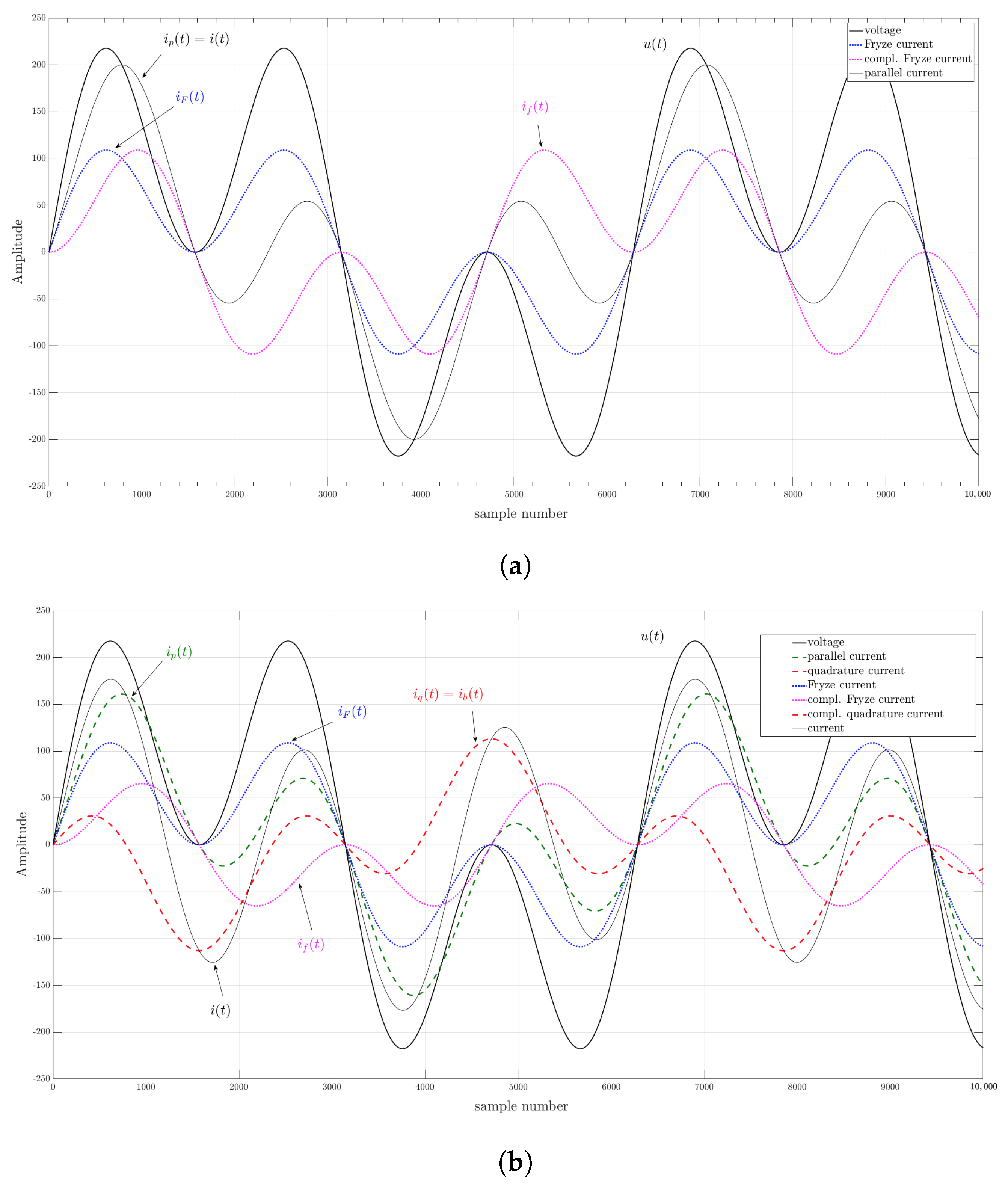
2.3. Current Decomposition

If $\overrightarrow{i}\left(t\right)$ is the instantaneous current demanded by a load, it can be separated into meaningful engineering components by manipulating (13) or (21) (depending on the nature of the load). For a linear load, left multiplying by the inverse of the voltage vector leads to:

$${\mathit{u}}^{-\mathbf{1}}\mathit{M}={\mathit{u}}^{-\mathbf{1}}\mathit{ui}=\mathit{i}$$

(23)

since ${\mathit{u}}^{-\mathbf{1}}\mathit{u}=1$. The inverse of a vector in GA is:

$${\mathit{u}}^{-\mathbf{1}}=\frac{\mathit{u}}{{\parallel \mathit{u}\parallel }^2}$$

(24)

which can be used in (23) to find the current decomposition. By replacing (14) in (23):

$$\begin{array}{cc}\hfill \mathit{i}& ={\mathit{u}}^{-\mathbf{1}}\mathit{M}=\frac{\mathit{u}}{{\parallel \mathit{u}\parallel }^2}\mathit{M}=\frac{\mathit{u}}{{\parallel \mathit{u}\parallel }^2}\left(M_p+{\mathit{M}}_q\right)=\frac{\mathit{u}}{{\parallel \mathit{u}\parallel }^2}{M}_p+\frac{\mathit{u}}{{\parallel \mathit{u}\parallel }^2}{\mathit{M}}_q={\mathit{i}}_p+{\mathit{i}}_q.\hfill \end{array}$$

(25)

The above expression resembles that of Shepherd and Zakikhani [52]. The term ${\mathit{i}}_p$ is commonly known as instantaneous geometric parallel current, while the term ${\mathit{i}}_q$ is the instantaneous geometric quadrature current and is orthogonal to ${\mathit{i}}_p$. It should be noted that ${\mathit{i}}_q$ is not a pure reactive current since it is not always related to energy oscillations in reactive elements such as inductors or capacitors [53]. In fact, it includes the effects generated by asymmetries of voltage sources and load unbalance.

The geometric counterpart of the Fryze current [10] is introduced here by means of GA:

$${\mathit{i}}_F=\frac{{\overline{M}}_p}{\parallel \overline{\mathit{u}}{\parallel }^2}\mathit{u}$$

(26)

where ${\overline{M}}_p$ is the mean value of the geometric parallel power and $\parallel \overline{\mathit{u}}\parallel$ is the RMS value of the geometric voltage. It can be computed as

$$\parallel \overline{\mathit{u}}\parallel =\sqrt{\frac{1}{n}\sum _{k=1}^n{u}_k}.$$

(27)

If no DC component is present simultaneously in voltage and current, then it can be readily demonstrated that ${\overline{M}}_p=2P$, where P is the active power. By virtue of (15), we have

$${\overline{M}}_p={\int }_0^T\left(\sum _{k=1}^n\left(u_k{i}_k+\mathcal{H}\left[u_k\right]\mathcal{H}\left[i_k\right]\right)\right)=P+P=2P.$$

(28)

Moreover, the reactive current defined by Budeanu and supported by Willems [54], Lev-Ari [16] and Jeltsema [55] (among others) can be defined in the geometric domain by taking the HT of the voltage vector signal (which basically corresponds to the HT of its coordinates):

$${\mathit{i}}_B=\frac{{\overline{M}}_q}{\parallel \overline{\mathit{u}}{\parallel }^2}\mathcal{H}\left[\mathit{u}\right]$$

(29)

where ${\overline{M}}_q$ is the mean value of the quadrature geometric power. Similarly to the geometric parallel power, ${\overline{M}}_q=2Q$, where Q is the reactive power defined by Budeanu. A proof of the relationship between Q and the HT of the voltage is provided in [55]. Therefore, the current expression can be fully decomposed by means of (25), as follows:

$$\begin{array}{cc}\hfill \mathit{i}& ={\mathit{u}}^{-\mathbf{1}}\mathit{M}=\frac{\mathit{u}}{{\parallel \mathit{u}\parallel }^2}\mathit{M}=\frac{\mathit{u}}{{\parallel \mathit{u}\parallel }^2}\left({\overline{M}}_p+(M_p-{\overline{M}}_p)+{\overline{\mathit{M}}}_q+(\overline{\mathit{M}}-{\overline{\mathit{M}}}_q)\right)\hfill \\ \hfill & ={\mathit{i}}_F+{\mathit{i}}_f+{\mathit{i}}_B+{\mathit{i}}_b\hfill \end{array}$$

(30)

where ${\mathit{i}}_f$ is the (geometric) Fryze complementary current required to conform the parallel current. Similarly, ${\mathit{i}}_b$ is the Budeanu complementary current required to conform the quadrature current. The asymmetry or unbalance current is included in ${\mathit{i}}_f$ and ${\mathit{i}}_b$. Note that the Fryze current is proportional to the voltage waveform while the Budeanu current is proportional to the Hilbert voltage waveform. The complementary components (Fryze and Budeanu) have no specific physical meaning, but economical purposes to minimise transmission losses. In the case of a non-linear load, only ${\mathit{M}}_{\Vert }$ should be used in (25) for current decomposition purposes. The total current becomes

$$\begin{array}{cc}\hfill \mathit{i}& ={\mathit{i}}_{\Vert }+{\mathit{i}}_{\perp }={\mathit{i}}_p+{\mathit{i}}_q+{\mathit{i}}_{\perp }={\mathit{i}}_F+{\mathit{i}}_f+{\mathit{i}}_B+{\mathit{i}}_b+{\mathit{i}}_{\perp }.\hfill \end{array}$$

(31)

This current decomposition is important for engineering purposes. It should be clearly stated that no physical meaning is assigned to currents that can be considered fictitious such as ${\mathit{i}}_f$ or ${\mathit{i}}_b$. The use of GA allows a natural and elegant decomposition of currents and can be convenient mathematically. The proposed methodology can be seamlessly applied to any distorted system since no constraints (up to periodicity) have been imposed on the waveforms of voltages and currents in this regard. This theory can be applied to any circuit with an arbitrary number of phases, including single-phase systems. This cannot be achieved by using other theories such as the $IRP$, and it is a relevant feature of this proposal.

The transformation from the geometric to the time domain for any current component included in ${\mathit{i}}_{\Vert }$ is axiomatically defined as:

$$\overrightarrow{i}\left(t\right)=\sum _{k=1}^n{\left[{\mathit{i}}_{\Vert }\right]}_k$$

(32)

where ${\left[X\right]}_k$ refers to the k-th term of the geometric vector of the in-band current ${\mathit{i}}_{\Vert }$.

3. Properties of the Geometric Power and Current

The instantaneous geometric power $\mathit{M}$ and the instantaneous geometric current $\mathit{i}$ fulfil a number of mathematical properties that reinforce the geometric interpretation of the proposed theory. Moreover, $\mathit{M}$ also provides some interesting physical and engineering insights. These ideas are explained below.

3.1. Orthogonality of Components in $\mathit{M}$

The parallel geometric power $M_p$ is a scalar number, while the quadrature geometric power ${\mathit{M}}_{\mathit{q}}$ is a bivector. Therefore, they have different grades and this implies orthogonality directly in GA. By definition, the norm of the instantaneous geometric power is:

$$\parallel \mathit{M}\parallel =\sqrt{{〈\mathit{M}{\mathit{M}}^{†}〉}_0}.$$

(33)

Therefore, the following relationship can be proven:

$$\begin{array}{cc}\hfill {\parallel \mathit{M}\parallel }^2& ={〈\left(M_p+{\mathit{M}}_q\right){\left(M_p+{\mathit{M}}_q\right)}^{†}〉}_0=\parallel M_p{\parallel }^2+{\parallel {\mathit{M}}_q\parallel }^2.\hfill \end{array}$$

Moreover, the norm of the geometric power also satisfies:

$$\parallel \mathit{M}\parallel =\parallel \mathit{u}\parallel \parallel \mathit{i}\parallel .$$

(34)

It can be readily proven by using the norm definition of a multi-vector and vector:

$$\begin{array}{cc}\hfill \parallel \mathit{M}\parallel & =\sqrt{{\langle {\mathit{M}}^{†}\mathit{M}\rangle }_0}=\sqrt{{\langle {\left(\mathit{ui}\right)}^{†}\left(\mathit{ui}\right)\rangle }_0}=\sqrt{{\langle \left({\mathit{i}}^{†}{\mathit{u}}^{†}\right)\left(\mathit{ui}\right)\rangle }_0}\hfill \\ & =\sqrt{{\parallel \mathit{u}\parallel }^2{\parallel \mathit{i}\parallel }^2}=\parallel \mathit{u}\parallel \parallel \mathit{i}\parallel .\hfill \end{array}$$

(35)

3.2. Conservative Property for $\mathit{M}$

The instantaneous geometric power $\mathit{M}$ is conservative and fulfils Tellegen’s theorem [56], which means that its sum over all components in a circuit is zero. This allows for identification of sources and sinks of reactive and non-active power, which may lead to allocation of compensation requirements.

3.3. Sign of the Quadrature Power ${\mathit{M}}_{\mathit{q}}$

The sign of ${\mathit{M}}_q$ provides useful information about the electrical characteristics of a load. Its value is positive for inductors, negative for capacitors and null for resistors.

3.4. Averaged Value of ${\mathit{M}}_{\mathit{q}}$

The averaged value of ${\mathit{M}}_q$ (${\overline{\mathit{M}}}_q$) is related to energy storage in inductors and capacitors (in the Budeanu sense) [54,55].

3.5. Orthogonality of Current Components

As shown in (25), the instantaneous geometric current $\mathit{i}$ can be decomposed into two vectors, ${\mathit{i}}_{\mathbf{p}}$ and ${\mathit{i}}_{\mathbf{q}}$. These vectors are indeed orthogonal. To prove the above statement, let us compute the quadrature current

$$\begin{array}{cc}\hfill {\mathit{i}}_q& ={\mathit{u}}^{-1}{\mathit{M}}_q={\mathit{u}}^{-1}·(\mathit{u}\wedge \mathit{i})+\underset{0}{\underbrace{{\mathit{u}}^{-1}\wedge (\mathit{u}\wedge \mathit{i})}}=-\left({\mathit{u}}^{-1}·\mathit{i}\right)\mathit{u}+\left({\mathit{u}}^{-1}·\mathit{u}\right)\mathit{i}\hfill \\ \hfill & =-\left({\mathit{u}}^{-1}·\mathit{i}\right)\mathit{u}+\mathit{i}=-\frac{M_p}{{\parallel \mathit{u}\parallel }^2}\mathit{u}+\mathit{i}=-M_p{\mathit{u}}^{-1}+\mathit{i}\hfill \end{array}$$

(36)

and the parallel current

$${\mathit{i}}_p=M_p{\mathit{u}}^{-1}.$$

(37)

Now, we test the orthogonality condition

$${\mathit{i}}_p·{\mathit{i}}_q=M_p{\mathit{u}}^{-1}·\left(-M_p{\mathit{u}}^{-1}+\mathit{i}\right)=-\frac{M_p^2}{{\parallel \mathit{u}\parallel }^2}+\frac{M_p^2}{{\parallel \mathit{u}\parallel }^2}=0.$$

(38)

Based on the same rationale, it can be proven that all the terms in (30) and (31) are orthogonal to each other. This fact establishes a solid framework for current reference in compensation applications such as passive or active filtering.

4. Instantaneous Geometric Impedance

For a linear load, the instantaneous relationship between in-band components of phase voltages and currents can be defined as the phase instantaneous geometric impedance. For a given phase k, the current and voltage can be represented either in Cartesian or polar coordinates as [26]:

$$\begin{array}{c}\hfill {\mathit{u}}_k=u_k{\mathbf{\sigma }}_k+\mathcal{H}\left[u_k\right]{\mathbf{\sigma }}_{\widehat{k}}=U_k{e}^{{\phi }_k^v{\mathbf{\sigma }}_{k\widehat{k}}}{\mathbf{\sigma }}_k\\ \hfill {\mathit{i}}_k=i_k{\mathbf{\sigma }}_k+\mathcal{H}\left[i_k\right]{\mathbf{\sigma }}_{\widehat{k}}=I_k{e}^{{\phi }_k^i{\mathbf{\sigma }}_{k\widehat{k}}}{\mathbf{\sigma }}_k\end{array}$$

(39)

where $e^{{\phi }_k^v{\mathbf{\sigma }}_{k\widehat{k}}}$ is a rotor, which is used to perform a rotation of $\phi$ degrees to vectors in the Argand plane ${\mathbf{\sigma }}_k-{\mathbf{\sigma }}_{\widehat{k}}$. Therefore:

$$\begin{array}{cc}\hfill {\mathbf{Z}}_k& ={\mathit{u}}_k{\mathit{i}}_k^{-1}=U_k{e}^{{\phi }_k^v{\mathbf{\sigma }}_{k\widehat{k}}}{\mathbf{\sigma }}_k{I}_k^{-1}{\mathbf{\sigma }}_k{e}^{-{\phi }_k^i{\mathbf{\sigma }}_{k\widehat{k}}}=\frac{U_k}{I_k}{e}^{({\phi }_k^v-{\phi }_k^i){\mathbf{\sigma }}_{k\widehat{k}}}\hfill \\ & =R_k+X_k{\mathbf{\sigma }}_{k\widehat{k}}=Z_k\angle {\phi }_k.\hfill \end{array}$$

(40)

In the above expression, $Z_k=U_k/I_k$ is the instantaneous impedance magnitude, ${\phi }_k={\phi }_k^v-{\phi }_k^i$ is the instantaneous phase, $R_k=Z_{k}cos{\phi }_k$ represents the instantaneous resistance and $X_k=Z_{k}sin{\phi }_k$ is the instantaneous reactance.

5. Examples

Two examples are detailed below to validate the proposal presented in this paper. Although they are theoretical examples, use in real environments with real-time or recorded data can be carried out without major issues. To this end, it is necessary to proceed with the proposed theory for each sample of voltage and current obtained by means of digital meters, such as the one proposed in [57]. For the symbolic computation of the proposed examples, the software Mathematica and WolframAlpha have been used, which has greatly simplified the calculations.

5.1. Example I: Single-Phase Circuit

Figure 2 shows two simple circuits commonly used in the literature to highlight how traditional power theories fail to provide satisfactory results for apparent power calculations. Consider now an extreme case of non-sinusoidal voltage supply such as $u\left(t\right)=100\sqrt{2}\left(sint+sin3t\right)$. It is not very common, but is used for illustrative purposes. The reactive powers (in the Budeanu sense) produced by each harmonic in the reactive elements are equal, but with opposite signs. Therefore, the total average reactive power is zero in both cases.

This problem has already been studied by using GA in the frequency domain [29]. It was proven that geometric power components can be clearly identified and, therefore, the geometric power value for each of the circuits in Figure 2 is different. Unfortunately, the use of complex algebra does not allow finding the interaction between voltage and current harmonics of different frequencies. In previous works, it was shown that (a) can be completely compensated by passive elements, but (b) requires an active compensator to achieve unity power factor. In this paper, the same circuits will be solved, but in the time domain.

5.1.1. Geometric Power Calculation

The geometric voltage and current vectors in the time domain are obtained by using (10):

$$\begin{array}{cc}\hfill \mathit{u}& =u\left(t\right){\mathbf{\sigma }}_1+\mathcal{H}\left[u\left(t\right)\right]{\mathbf{\sigma }}_{\widehat{1}}\hfill \\ \hfill \mathit{i}& =i\left(t\right){\mathbf{\sigma }}_1+\mathcal{H}\left[i\left(t\right)\right]{\mathbf{\sigma }}_{\widehat{1}}.\hfill \end{array}$$

The current waveforms for circuits (a) and (b) are:

$$\begin{array}{cc}\hfill i_a& =50\sqrt{2}\left(sint+cost+sin3t-cos3t\right)\hfill \\ \hfill i_b& =\sqrt{2}\left(10sint+30cost+90sin3t-30cos3t\right).\hfill \end{array}$$

From now on, sub-indexes a and b stand for circuit (a) and (b), respectively. The voltage and currents in the geometric domain are:

$$\begin{array}{cc}\hfill \mathit{u}& =100\sqrt{2}\left(sint+sin3t\right){\mathbf{\sigma }}_1+100\sqrt{2}\left(cost+cos3t\right){\mathbf{\sigma }}_{\widehat{1}}\hfill \\ \hfill {\mathit{i}}_a& =50\sqrt{2}\left(sint+cost+sin3t-cos3t\right){\mathbf{\sigma }}_1+50\sqrt{2}\left(cost-sint+cos3t+sin3t\right){\mathbf{\sigma }}_{\widehat{1}}\hfill \\ \hfill {\mathit{i}}_b& =\sqrt{2}\left(10sint+30cost+90sin3t-30cos3t\right){\mathbf{\sigma }}_1+\sqrt{2}\left(10cost-30sint+90cos3t+30sin3t\right){\mathbf{\sigma }}_{\widehat{1}}.\hfill \end{array}$$

The geometric power can be calculated with (13), yielding

$$\begin{array}{cc}\hfill {\mathit{M}}_a& =M_p^a+{\mathit{M}}_q^a=\underset{M_p^a}{\underbrace{\mathrm{20,000}\left(1+sin2t+cos2t\right)}}\hfill \\ \hfill {\mathit{M}}_b& =M_p^b+{\mathit{M}}_q^b=\underset{M_p^b}{\underbrace{\mathrm{20,000}+\mathrm{12,000}sin2t+\mathrm{20,000}cos2t}}-\underset{{\mathit{M}}_q^b}{\underbrace{\mathrm{16,000}sin2t{\mathbf{\sigma }}_{1\widehat{1}}}}.\hfill \end{array}$$

In both cases, the active power is $P={\overline{\mathit{M}}}_p/2=\mathrm{10,000}$ W. However, for the quadrature geometric power ${\mathit{M}}_q^a=0$ while ${\mathit{M}}_q^b\ne 0$. From a practical point of view, this implies that circuit (b) would need active filtering elements in order to achieve unit power factor. In both circuits, the reactive power (in the Budeanu sense) is $Q={\overline{M}}_q/2=0$. Therefore, it is impossible to compute the required passive compensation in the time domain. In this case, a frequency domain approach should be used to calculate the contribution of each harmonic (one by one) to the geometric power [26].

5.1.2. Current Decomposition

The current can be decomposed by using the expressions (25)–(30). In order to use them, the inverse of the voltage vector should be calculated:

$${\mathit{u}}^{-1}=\frac{\mathit{u}}{{\parallel \mathit{u}\parallel }^2}=\frac{sint}{100\sqrt{2}}{\mathbf{\sigma }}_1+\frac{cos2t}{200\sqrt{2}cost}{\mathbf{\sigma }}_{\widehat{1}}$$

where

$$\begin{array}{cc}\hfill {\parallel \mathit{u}\parallel }^2& ={\left(100\sqrt{2}\left(sint+sin3t\right)\right)}^2+{\left(100\sqrt{2}\left(cost+cos3t\right)\right)}^2\hfill \\ \hfill & =\mathrm{80,000}{(cost)}^2=\mathrm{40,000}(cos2t+1).\hfill \end{array}$$

We can now compute the currents accordingly

$$\begin{array}{cccc}\hfill {\mathit{i}}_p& =\frac{\mathit{u}}{{\parallel \mathit{u}\parallel }^2}{M}_p\hfill & \hfill {\mathit{i}}_q& =\frac{\mathit{u}}{{\parallel \mathit{u}\parallel }^2}{\mathit{M}}_{\mathit{q}}\hfill \\ \hfill {\mathit{i}}_F& =\frac{{\overline{M}}_p}{\parallel \overline{\mathit{u}}{\parallel }^2}\mathit{u}\hfill & \hfill {\mathit{i}}_f& ={\mathit{i}}_p-{\mathit{i}}_F\hfill \\ \hfill {\mathit{i}}_B& =\frac{{\overline{M}}_q}{\parallel \overline{\mathit{u}}{\parallel }^2}\mathcal{H}\left[\mathit{u}\right]\hfill & \hfill {\mathit{i}}_b& ={\mathit{i}}_q-{\mathit{i}}_B.\hfill \end{array}$$

The current components obtained by using this procedure are shown in

Table 1. Current decomposition for circuit in Figure 2. The column for component ${\mathbf{\sigma }}_1$ represents the real current in the circuit while ${\mathbf{\sigma }}_{\widehat{1}}$ is the quadrature signal after applying the HT. The last column accounts for the RMS value of the real current.

Vector
		${\mathbf{\sigma }}_1$	${\mathbf{\sigma }}_{\widehat{1}}$	$\parallel {\mathbf{\sigma }}_1\parallel$
${\mathit{i}}_p$	(a)	$\sqrt{2}\left(50sint+50cost+50sin3t-50cos3t\right)$	$\sqrt{2}\left(50cost-50sint+50cos3t+50sin3t\right)$	100.00
	(b)	$\sqrt{2}\left(50sint+30cost+50sin3t-30cos3t\right)$	$\sqrt{2}\left(50cost-30sint+50cos3t+30sin3t\right)$	82.45
${\mathit{i}}_q$	(a)	0.00	0.00	0.00
	(b)	$\sqrt{2}\left(-40sint+40sin3t\right)$	$\sqrt{2}\left(-40cost+40cos3t\right)$	56.56
${\mathit{i}}_F$	(a)	$\sqrt{2}\left(50sint+50sin3t\right)$	$\sqrt{2}\left(50cost+50cos3t\right)$	70.71
	(b)	$\sqrt{2}\left(50sint+50sin3t\right)$	$\sqrt{2}\left(50cost+50cos3t\right)$	70.71
${\mathit{i}}_f$	(a)	$\sqrt{2}\left(50cost-50cos3t\right)$	$\sqrt{2}\left(-50sint+50sin3t\right)$	70.71
	(b)	$\sqrt{2}\left(30cost-30cos3t\right)$	$\sqrt{2}\left(-30sint+30sin3t\right)$	42.42
${\mathit{i}}_B$	(a)	$0.00$	$0.00$	0.00
	(b)	$0.00$	$0.00$	0.00
${\mathit{i}}_b$	(a)	$0.00$	$0.00$	0.00
	(b)	$\sqrt{2}\left(-40sint+40sin3t\right)$	$\sqrt{2}\left(-40cost+40cos3t\right)$	56.56
$\mathit{i}$	(a)	$\sqrt{2}\left(50sint+50cost+50sin3t-50cos3t\right)$	$\sqrt{2}\left(50cost-50sint+50cos3t+50sin3t\right)$	100.00
	(b)	$\sqrt{2}\left(10sint+30cost+90sin3t-30cos3t\right)$	$\sqrt{2}\left(10cost-30sint+90cos3t+30sin3t\right)$	100.00

. This composition clearly highlights the differences between the two circuits. First, it can be seen that even though the norm is the same, the waveforms differ among them. The parallel current ${\mathit{i}}_p$ for circuit (a) is slightly lower compared to that of circuit (b). The Fryze current ${\mathit{i}}_F$ is the same for both circuits because the active power consumption P is also the same. In both circuits, the current ${\mathit{i}}_B$ is zero. This confirms that it is not possible to compensate their current only with passive elements using the time domain approach. Figure 3 shows the current components for both circuits where the differences can be clearly observed. Currents in the time domain can be recovered by using (32).

5.1.3. Geometric Impedance Calculation

The instantaneous impedance of the circuit can be calculated by using (40):

$$\mathit{Z}=\mathit{u}{\mathit{i}}^{-1}=\mathit{u}\frac{\mathit{i}}{{\parallel \mathit{i}\parallel }^2}=\frac{\mathit{M}}{{\parallel \mathit{i}\parallel }^2}.$$

Therefore, for circuits (a) and (b), it follows that

$$\begin{array}{cc}\hfill {\mathit{Z}}_a& =1+\frac{cos2t}{1+sin2t}\hfill \\ \hfill {\mathit{Z}}_b& =1+\frac{5cos2t}{5+3sin2t}-\frac{4sin2t}{5+3sin2t}{\mathbf{\sigma }}_{1\widehat{1}}.\hfill \end{array}$$

The two circuits have different behaviours because their instantaneous impedances are also different. It can be seen that circuit (a) does not have instantaneous reactance, while circuit (b) does. Resistive parts also differ.

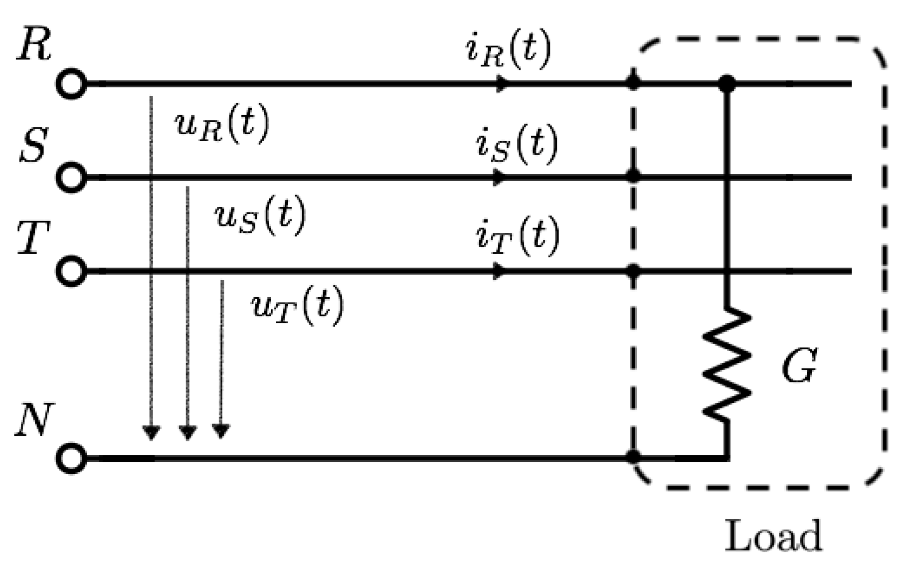
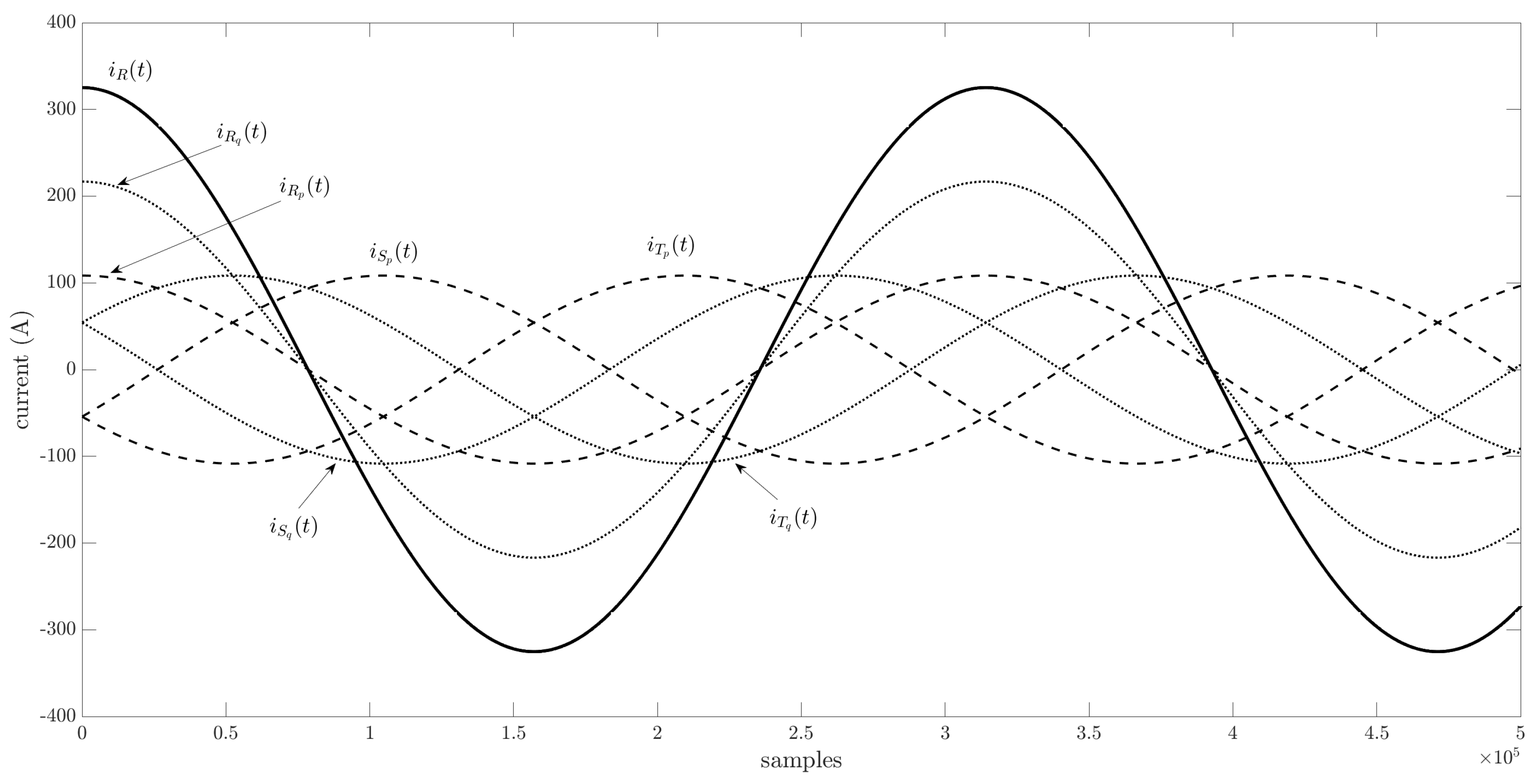
5.2. Example II: Unbalanced Three-Phase Circuit

Figure 4 shows a circuit that has been used by several authors to highlight the weaknesses of the $IRP$ theory [4,22]. Only the instantaneous approach is used in the $IRP$ theory. Therefore, some results might be considered senseless or even erroneous. However, this theory is widely used for instantaneous current compensation. If the proposed theory in this paper is used, but omitting the HT (10) representation, the results would be similar to those obtained with the $IRP$ theory. This suggests that cross product theories are a subset of the GA formulation, where the traditional cross vector product is used instead of the more general exterior product. In fact, in a three-dimensional space, the resulting vector $\mathit{a}=\mathit{b}\times \mathbf{c}$ can be expressed as the dual of the wedge product as $\mathit{a}=-I\mathit{b}\wedge \mathbf{c}$, with $I={\mathbf{\sigma }}_1{\mathbf{\sigma }}_2{\mathbf{\sigma }}_3$. Unfortunately, the cross product only yields unique orthogonal vectors in three-dimensional spaces and this limits its applicability. In contrast, the proposed theory can be used for any number of dimensions, i.e., electrical phases. For a three-phase system, the voltage and current vectors are

$$\begin{array}{cc}\hfill \mathit{u}& =u_R{\mathbf{\sigma }}_1+u_S{\mathbf{\sigma }}_2+u_T{\mathbf{\sigma }}_3\hfill \\ \hfill \mathit{i}& =i_R{\mathbf{\sigma }}_1+i_S{\mathbf{\sigma }}_2+i_T{\mathbf{\sigma }}_3.\hfill \end{array}$$

If the instantaneous approach is used, the current decomposition procedure is similar to the previous single-phase circuit by applying (13). However, if we apply (10), where the HT is incorporated, the results would be more consistent from the electrical point of view and it would be possible to calculate the minimum current (in the Fryze sense).

In the circuit of Figure 4, the supply voltage is balanced and sinusoidal:

$$\begin{array}{c}{u}_R\left(t\right)=\sqrt{2}Ucos\omega t\hfill \\ u_S\left(t\right)=\sqrt{2}Ucos\left(\omega t-120\right)\hfill \\ u_T\left(t\right)=\sqrt{2}Ucos\left(\omega t+120\right).\hfill \end{array}$$

Only the current of the phase R is not null. Therefore:

$$i_R\left(t\right)=\sqrt{2}GUcos\omega t.$$

The instantaneous geometric voltage and current vectors are obtained as:

$$\begin{array}{cc}\hfill \mathit{u}& =\sqrt{2}U[cos\omega t{\mathbf{\sigma }}_1-sin\omega t{\mathbf{\sigma }}_{\widehat{1}}+cos\left(\omega t-120\right){\mathbf{\sigma }}_2-sin\left(\omega t-120\right){\mathbf{\sigma }}_{\widehat{2}}+cos\left(\omega t+120\right){\mathbf{\sigma }}_3\hfill \\ \hfill & -sin\left(\omega t+120\right){\mathbf{\sigma }}_{\widehat{3}}]\hfill \\ \hfill \mathit{i}& =\sqrt{2}GU[cos\omega t{\mathbf{\sigma }}_1-sin\omega t{\mathbf{\sigma }}_{\widehat{1}}]\hfill \end{array}$$

and the geometric power is:

$$\begin{array}{cc}\mathit{M}\hfill & =\mathit{ui}=2G{U}^2\left[1-cos\omega tcos\left(\omega t-120\right){\mathbf{\sigma }}_{12}\right.\hfill \\ \hfill & +cos\omega tsin\left(\omega t+120\right){\mathbf{\sigma }}_{1\widehat{2}}-cos\omega tcos\left(\omega t+120\right){\mathbf{\sigma }}_{13}\hfill \\ \hfill & +cos\omega tsin\left(\omega t+120\right){\mathbf{\sigma }}_{1\widehat{3}}-sin\omega tcos\left(\omega t-120\right){\mathbf{\sigma }}_{\widehat{1}2}\hfill \\ \hfill & +sin\omega tsin\left(\omega t-120\right){\mathbf{\sigma }}_{\widehat{1}\widehat{2}}-sin\omega tcos\left(\omega t+120\right){\mathbf{\sigma }}_{\widehat{1}3}\hfill \\ \hfill & \left.+sin\omega tsin\left(\omega t+120\right){\mathbf{\sigma }}_{\widehat{1}\widehat{3}}\right].\hfill \end{array}$$

In this expression, the geometric parallel power is constant and its value is $M_p=2G{U}^2$. This looks reasonable since the circuit is purely resistive and the demanded active power is $P=G{U}^2={\overline{M}}_p/2$. The other power terms are related to the unbalance components of the load, being bivectors by nature. Note that ${\mathbf{\sigma }}_{1\widehat{1}}$, ${\mathbf{\sigma }}_{2\widehat{2}}$ and ${\mathbf{\sigma }}_{3\widehat{3}}$ are not present in this expression. This means that there is no reactive power in the Budeanu sense. This is also reasonable since there are no inductive nor capacitive elements in this simple linear circuit. The current decomposition can now be obtained according to (25)–(30). Considering that ${\parallel \mathit{u}\parallel }^2=6U^2$:

$$\begin{array}{cc}\hfill {\mathit{i}}_p& =\frac{\mathit{u}}{{\parallel \mathit{u}\parallel }^2}{M}_p=\frac{G}{3}\mathit{u}=\sqrt{2}\frac{GU}{3}[cos\omega t{\mathbf{\sigma }}_1-sin\omega t{\mathbf{\sigma }}_{\widehat{1}}+cos\left(\omega t-120\right){\mathbf{\sigma }}_2\hfill \\ \hfill & -sin\left(\omega t-120\right){\mathbf{\sigma }}_{\widehat{2}}+cos\left(\omega t+120\right){\mathbf{\sigma }}_3-sin\left(\omega t+120\right){\mathbf{\sigma }}_{\widehat{3}}]\hfill \\ \hfill {\mathit{i}}_q& =\frac{\mathit{u}}{{\parallel \mathit{u}\parallel }^2}{\mathit{M}}_q=\mathit{i}-{\mathit{i}}_p=\sqrt{2}\frac{GU}{3}[2cos\omega t{\mathbf{\sigma }}_1-2sin\omega t{\mathbf{\sigma }}_{\widehat{1}}-cos\left(\omega t-120\right){\mathbf{\sigma }}_2\hfill \\ \hfill & +sin\left(\omega t-120\right){\mathbf{\sigma }}_{\widehat{2}}-cos\left(\omega t+120\right){\mathbf{\sigma }}_3+sin\left(\omega t+120\right){\mathbf{\sigma }}_{\widehat{3}}].\hfill \end{array}$$

For this example, the Fryze current matches the parallel current $({\mathit{i}}_p={\mathit{i}}_F)$. Therefore, ${\mathit{i}}_f=0$. Additionally, there is no reactive current (in the Budeanu sense) since ${\overline{M}}_q=0$, and therefore, ${\mathit{i}}_B=0$. It can be seen that ${\mathit{i}}_b={\mathit{i}}_q$. This means that this current contains all the asymmetrical components, which include both zero sequence current ${\mathit{i}}_0$ and negative sequence current ${\mathit{i}}_{-}$:

$${\mathit{i}}_q={\mathit{i}}_b={\mathit{i}}_0+{\mathit{i}}_{-}$$

where

$$\begin{array}{cc}\hfill {\mathit{i}}_0& =\sqrt{2}\frac{GU}{3}[cos\omega t{\mathbf{\sigma }}_1-sin\omega t{\mathbf{\sigma }}_{\widehat{1}}+cos\omega t{\mathbf{\sigma }}_2-sin\omega t{\mathbf{\sigma }}_{\widehat{2}}+cos\omega t{\mathbf{\sigma }}_3-sin\omega t{\mathbf{\sigma }}_{\widehat{3}}]\hfill \\ \hfill {\mathit{i}}_{-}& =\sqrt{2}\frac{GU}{3}[cos\omega t{\mathbf{\sigma }}_1-sin\omega t{\mathbf{\sigma }}_{\widehat{1}}+cos\left(\omega t+120\right){\mathbf{\sigma }}_2-sin\left(\omega t+120\right){\mathbf{\sigma }}_{\widehat{2}}\hfill \\ \hfill & +cos\left(\omega t-120\right){\mathbf{\sigma }}_3-sin\left(\omega t-120\right){\mathbf{\sigma }}_{\widehat{3}}].\hfill \end{array}$$

Figure 5 shows the current decomposition for $U=230$ V, $\omega =1$ rad/s and $G=1$ Ohm. The time domain current is obtained by applying (32) to the geometric vector

$$i_p\left(t\right)=\left[\begin{array}{c}{i}_{R_p}\left(t\right)\\ i_{S_p}\left(t\right)\\ i_{T_p}\left(t\right)\end{array}\right]=\frac{\sqrt{2}GU}{3}\left[\begin{array}{c}cos\omega t\\ cos\left(\omega t-120\right)\\ cos\left(\omega t+120\right)\end{array}\right]$$

$$i_q\left(t\right)=\left[\begin{array}{c}{i}_{R_q}\left(t\right)\\ i_{S_q}\left(t\right)\\ i_{T_q}\left(t\right)\end{array}\right]=\frac{\sqrt{2}GU}{3}\left[\begin{array}{c}2cos\omega t\\ -cos\left(\omega t-120\right)\\ -cos\left(\omega t+120\right)\end{array}\right]=\underset{i_0\left(t\right)}{\underbrace{\frac{\sqrt{2}GU}{3}\left[\begin{array}{c}cos\omega t\\ cos\omega t\\ cos\omega t\end{array}\right]}}+\underset{i_{-}\left(t\right)}{\underbrace{\frac{\sqrt{2}GU}{3}\left[\begin{array}{c}cos\omega t\\ cos\left(\omega t+120\right)\\ cos\left(\omega t-120\right)\end{array}\right]}}.$$

6. Conclusions

In this paper, power definitions and computations for multi-phase electrical circuits in a mixed time–frequency domain have been addressed by using geometric algebra and the Hilbert transform. It has been shown that our proposal greatly simplifies the plethora of mathematical tools to a unified approach, leading to a compact formulation. Moreover, it establishes a new framework that can be applied under any supply or load condition. The proposed formulation can be used in both single- and multi-phase systems and it provides a robust interpretation that is in good agreement with electrical engineering evidence. Current decomposition can be carried out as the inverse operation. The results highlight the validity of the methodology, which has been verified in electrical circuits previously proposed in the literature. Further research will focus on the application of this theory for calculating power flows in distorted electrical networks with non-linear loads.

References

1. Steinmetz, C.P. Complex quantities and their use in electrical engineering. In Proceedings of the International Electrical Congress, Chicago, IL, USA, 21–25 August 1893; pp. 33–74. [Google Scholar]
2. Kennelly, A. Impedance. Trans. Am. Inst. Electr. Eng. 1893, 10, 172–232. [Google Scholar] [CrossRef]
3. Heaviside, O. Electrical Papers; Macmillan and Company: Troon, UK, 1892; Volume 2. [Google Scholar]
4. Czarnecki, L.S. Instantaneous reactive power p-q theory and power properties of three-phase systems. IEEE Trans. Power Deliv. 2005, 21, 362–367. [Google Scholar] [CrossRef]
5. Malengret, M.; Gaunt, C.T. Active currents, power factor, and apparent power for practical power delivery systems. IEEE Access 2020, 8, 133095–133113. [Google Scholar] [CrossRef]
6. Cohen, J.; De Leon, F.; Hernández, L.M. Physical time domain representation of powers in linear and nonlinear electrical circuits. IEEE Trans. Power Deliv. 1999, 14, 1240–1249. [Google Scholar] [CrossRef]
7. Cristaldi, L.; Ferrero, A. Mathematical foundations of the instantaneous power concepts: An algebraic approach. Eur. Trans. Electr. Power 1996, 6, 305–309. [Google Scholar] [CrossRef]
8. Budeanu, C. Puissances Reactives et Fictives; Number 2; Impr. Cultura Nationala: Bucuresti, Romania, 1927. [Google Scholar]
9. Czarnecki, L.S. Currents’ physical components (CPC) concept: A fundamental of power theory. In Proceedings of the International School on Nonsinusoidal Currents and Compensation, Lagow, Poland, 10–13 June 2008; pp. 1–11. [Google Scholar]
10. Fryze, S. Wirk-, Blind-und Scheinleistung in elektrischen Stromkreisen mit nichtsinusförmigem Verlauf von Strom und Spannung. Elektrotechnische Z. 1932, 25, 33. [Google Scholar]
11. Akagi, H.; Kanazawa, Y.; Nabae, A. Instantaneous reactive power compensators comprising switching devices without energy storage components. IEEE Trans. Ind. Appl. 1984, IA-20, 625–630. [Google Scholar] [CrossRef]
12. Depenbrock, M. The FBD-method, a generally applicable tool for analyzing power relations. IEEE Trans. Power Syst. 1993, 8, 381–387. [Google Scholar] [CrossRef]
13. Staudt, V. Fryze-Buchholz-Depenbrock: A time-domain power theory. In Proceedings of the International School on Nonsinusoidal Currents and Compensation, Lagow, Poland, 10–13 June 2008; pp. 1–12. [Google Scholar]
14. Peng, F.Z.; Lai, J.S. Generalized instantaneous reactive power theory for three-phase power systems. IEEE Trans. Instrum. Meas. 1996, 45, 293–297. [Google Scholar] [CrossRef] [Green Version]
15. Dai, X.; Liu, G.; Gretsch, R. Generalized theory of instantaneous reactive quantity for multiphase power system. IEEE Trans. Power Deliv. 2004, 19, 965–972. [Google Scholar] [CrossRef]
16. Lev-Ari, H.; Stankovic, A.M. A decomposition of apparent power in polyphase unbalanced networks in nonsinusoidal operation. IEEE Trans. Power Syst. 2006, 21, 438–440. [Google Scholar] [CrossRef]
17. Salmerón, P.; Herrera, R. Instantaneous reactive power theory—A general approach to poly-phase systems. Electr. Power Syst. Res. 2009, 79, 1263–1270. [Google Scholar] [CrossRef]
18. Ustariz, A.; Cano, E.; Tacca, H. Tensor analysis of the instantaneous power in electrical networks. Electr. Power Syst. Res. 2010, 80, 788–798. [Google Scholar] [CrossRef]
19. Ustariz-Farfan, A.; Cano-Plata, E.; Tacca, H.; Garces-Gomez, Y. Hybrid simulation to test control strategies in active power filters using generalized power tensor theory. In Proceedings of the 2012 IEEE 15th International Conference on Harmonics and Quality of Power, Hong Kong, China, 17–20 June 2012; pp. 598–604. [Google Scholar]
20. Mirzakhani, A.; Ghandehari, R.; Davari, S.A. Performance improvement of DPC in DFIGs during unbalanced grid voltage based on extended power theory. Ain Shams Eng. J. 2021, 12, 1775–1786. [Google Scholar] [CrossRef]
21. Sriranjani, R.; Jayalalitha, S. Instantaneous d frame driven shunt active filter for harmonics and reactive power mitigation using Xilinx System Generator. Ain Shams Eng. J. 2019, 10, 15–22. [Google Scholar] [CrossRef]
22. Haley, P. Limitations of cross vector generalized pq theory. In Proceedings of the 2015 International School on Nonsinusoidal Currents and Compensation (ISNCC), Lagow, Poland, 15–18 June 2015; pp. 1–5. [Google Scholar]
23. Salmeron, P.; Herrera, R.S. Distorted and unbalanced systems compensation within instantaneous reactive power framework. IEEE Trans. Power Deliv. 2006, 21, 1655–1662. [Google Scholar] [CrossRef]
24. Herrera, R.; Salmeron, P. Present point of view about the instantaneous reactive power theory. IET Power Electron. 2009, 2, 484–495. [Google Scholar] [CrossRef]
25. Montoya, F.G.; Baños, R.; Alcayde, A.; Arrabal-Campos, F.M.; Roldán Pérez, J. Geometric Algebra Framework Applied to Symmetrical Balanced Three-Phase Systems for Sinusoidal and Non-Sinusoidal Voltage Supply. Mathematics 2021, 9, 1259. [Google Scholar] [CrossRef]
26. Montoya, F.G.; Baños, R.; Alcayde, A.; Arrabal-Campos, F.M.; Roldán-Pérez, J. Vector Geometric Algebra in Power Systems: An Updated Formulation of Apparent Power under Non-Sinusoidal Conditions. Mathematics 2021, 9, 1295. [Google Scholar] [CrossRef]
27. Arsenovic, A. Applications of conformal geometric algebra to transmission line theory. IEEE Access 2017, 5, 19920–19941. [Google Scholar] [CrossRef]
28. Liu, L.W.; Hong, H.K. Clifford algebra valued boundary integral equations for three-dimensional elasticity. Appl. Math. Model. 2018, 54, 246–267. [Google Scholar] [CrossRef]
29. Montoya, F.G.; Baños, R.; Alcayde, A.; Arrabal-Campos, F.M.; Viciana, E. Analysis of non-active power in non-sinusoidal circuits using geometric algebra. Int. J. Electr. Power Energy Syst. 2020, 116, 105541. [Google Scholar] [CrossRef]
30. Lev-Ari, H.; Stankovic, A.M. Instantaneous power quantities in polyphase systems—A geometric algebra approach. In Proceedings of the 2009 IEEE Energy Conversion Congress and Exposition, San Jose, CA, USA, 20–24 September 2009; pp. 592–596. [Google Scholar]
31. De Leon, F.; Cohen, J. Discussion of “Generalized theory of instantaneous reactive quantity for multiphase power system”. IEEE Trans. Power Deliv. 2005, 21, 540–541. [Google Scholar] [CrossRef]
32. Montoya, F.G.; De Leon, F.; Arrabal-Campos, F.M.; Alcayde, A. Determination of Instantaneous Powers from a Novel Time-Domain Parameter Identification Method of Non-Linear Single-Phase Circuits. IEEE Trans. Power Deliv. 2021, 1. [Google Scholar] [CrossRef]
33. Saitou, M.; Shimizu, T. Generalized theory of instantaneous active and reactive powers in single-phase circuits based on Hilbert transform. In Proceedings of the 2002 IEEE 33rd Annual IEEE Power Electronics Specialists Conference. Proceedings (Cat. No. 02CH37289), Cairns, Australia, 23–27 June 2002; Volume 3, pp. 1419–1424. [Google Scholar]
34. Nowomiejski, Z. Generalized theory of electric power. Arch. Elektrotechnik 1981, 63, 177–182. [Google Scholar] [CrossRef]
35. Herrera, R.S.; Salmerón, P.; Kim, H. Instantaneous reactive power theory applied to active power filter compensation: Different approaches, assessment, and experimental results. IEEE Trans. Ind. Electron. 2008, 55, 184–196. [Google Scholar] [CrossRef]
36. Rockhill, A.; Lipo, T. A generalized transformation methodology for polyphase electric machines and networks. In Proceedings of the 2015 IEEE International Electric Machines & Drives Conference (IEMDC), Coeur d’Alene, ID, USA, 10–13 May 2015; pp. 27–34. [Google Scholar]
37. Wu, J.C. Novel circuit configuration for compensating for the reactive power of induction generator. IEEE Trans. Energy Convers. 2008, 23, 156–162. [Google Scholar]
38. Chakraborty, S.; Simoes, M.G. Experimental evaluation of active filtering in a single-phase high-frequency AC microgrid. IEEE Trans. Energy Convers. 2009, 24, 673–682. [Google Scholar] [CrossRef]
39. Rim, C.T. Unified general phasor transformation for AC converters. IEEE Trans. Power Electron. 2011, 26, 2465–2475. [Google Scholar] [CrossRef]
40. Chappell, J.M.; Drake, S.P.; Seidel, C.L.; Gunn, L.J.; Iqbal, A.; Allison, A.; Abbott, D. Geometric algebra for electrical and electronic engineers. Proc. IEEE 2014, 102, 1340–1363. [Google Scholar] [CrossRef]
41. Chappell, J.M.; Iqbal, A.; Hartnett, J.G.; Abbott, D. The vector algebra war: A historical perspective. IEEE Access 2016, 4, 1997–2004. [Google Scholar] [CrossRef] [Green Version]
42. Hestenes, D.; Sobczyk, G. Clifford Algebra to geometric Calculus: A Unified Language for Mathematics and Physics; Springer Science & Business Media: Berlin, Germany, 2012; Volume 5. [Google Scholar]
43. Josipovic, M. Geometric Multiplication of Vectors; Springer: Berlin, Germany, 2019. [Google Scholar]
44. Felsberg, M.; Sommer, G. The monogenic signal. IEEE Trans. Signal Process. 2001, 49, 3136–3144. [Google Scholar] [CrossRef] [Green Version]
45. Bracewell, R.N.; Bracewell, R.N. The Fourier Transform and Its Applications; McGraw-Hill: New York, NY, USA, 1986; Volume 31999. [Google Scholar]
46. Babu, N.R.; Mohan, B.J. Fault classification in power systems using EMD and SVM. Ain Shams Eng. J. 2017, 8, 103–111. [Google Scholar] [CrossRef] [Green Version]
47. Kschischang, F.R. The hilbert transform. Univ. Tor. 2006, 83, 277. [Google Scholar]
48. Hahn, S.L.; Snopek, K.M. Complex and Hypercomplex Analytic Signals: Theory and Applications; Artech House: London, UK, 2016. [Google Scholar]
49. Gibbs, J.W. Vector Analysis: A Text-Book for the Use of Students of Mathematics and Physics, Founded upon the Lectures of j. Willard Gibbs; Yale University Press: London, UK, 1901. [Google Scholar]
50. Willems, J.L. A new interpretation of the Akagi-Nabae power components for nonsinusoidal three-phase situations. IEEE Trans. Instrum. Meas. 1992, 41, 523–527. [Google Scholar] [CrossRef]
51. Akagi, H.; Watanabe, E.H.; Aredes, M. Instantaneous Power Theory and Applications to Power Conditioning; Wiley: Hoboken, NJ, USA, 2007. [Google Scholar]
52. Shepherd, W.; Zakikhani, P. Suggested definition of reactive power for nonsinusoidal systems. Proc. Inst. Electr. Eng. 1972, 119, 1361–1362. [Google Scholar] [CrossRef]
53. De Leon, F.; Cohen, J. AC power theory from Poynting theorem: Accurate identification of instantaneous power components in nonlinear-switched circuits. IEEE Trans. Power Deliv. 2010, 25, 2104–2112. [Google Scholar] [CrossRef]
54. Willems, J.L. Budeanu’s reactive power and related concepts revisited. IEEE Trans. Instrum. Meas. 2010, 60, 1182–1186. [Google Scholar] [CrossRef]
55. Jeltsema, D. Budeanu’s concept of reactive and distortion power revisited. In Proceedings of the 2015 IEEE International School on Nonsinusoidal Currents and Compensation (ISNCC), Lagow, Poland, 15–18 June 2015; pp. 1–6. [Google Scholar]
56. Castro-Núñez, M.; Londoño-Monsalve, D.; Castro-Puche, R. M, the conservative power quantity based on the flow of energy. J. Eng. 2016, 2016, 269–276. [Google Scholar] [CrossRef]
57. Viciana, E.; Alcayde, A.; Montoya, F.G.; Baños, R.; Arrabal-Campos, F.M.; Manzano-Agugliaro, F. An open hardware design for internet of things power quality and energy saving solutions. Sensors 2019, 19, 627. [Google Scholar] [CrossRef] [Green Version]
Figure 1. Representation of an n-phase, ( n + 1 )-wire circuit with virtual star point N. Line to virtual neutral point voltages and line currents are depicted.
Mathematics 10 01419 g001
Figure 2. Two R L C circuits are used for Example I. They are very similar (same series R L C ) but differ in the values of the capacitor, i.e., C = 2 / 3 F for circuit (a) and C = 2 / 7 F for circuit (b), so the reactive power provided by the source is also different.
Mathematics 10 01419 g002
Figure 3. Currents in time domain for the circuits in Figure 2. The signals for circuit (a) are shown at the top and the values for circuit (b) at the bottom. Time samples are depicted on the x axis and amplitude of current/voltage on the y axis.
Mathematics 10 01419 g003
Figure 4. Unbalanced three-phase load supplied by a symmetrical souce in a four-wire circuit.
Mathematics 10 01419 g004
Figure 5. Current decomposition for the three-phase circuit. The very unbalanced system of currents (solid line) can be decomposed in 3 symmetrical sets of currents, i p , i 0 and i .
Mathematics 10 01419 g005