
Stress State in an Eccentric Elastic Ring Loaded Symmetrically by Concentrated Forces

Mechanics and Technologies Department, Faculty of Mechanical Engineering, Automotive and Robotics, Stefan cel Mare University of Suceava, 720229 Suceava, Romania
*
Authors to whom correspondence should be addressed.
Mathematics 2022, 10(8), 1314; https://doi.org/10.3390/math10081314
Submission received: 4 March 2022
/
Revised: 7 April 2022
/
Accepted: 12 April 2022
/
Published: 14 April 2022
(This article belongs to the Topic Engineering Mathematics)
Abstract
:The stress state from an eccentric ring made of an elastic material symmetrically loaded on the outer boundary by concentrated forces is deduced. The analytical results are obtained using the Airy stress function expressed in bipolar coordinates. The elastic potential corresponding to the same loading but for a compact disk is first written in bipolar coordinates, then expanded in Fourier series, and after that, an auxiliary potential of a convenient form is added to it in order to impose boundary conditions. Since the inner boundary is unloaded, boundary conditions may be applied directly to the total potential. A special focus is on the number of terms from Fourier expansion of the potential in bipolar coordinates corresponding to the compact disk as this number influences the sudden increase if the coefficients from the final form of the total potential. Theoretical results are validated both by using finite element software and experimentally through the photoelastic method, for which a device for sample loading was designed and constructed. Isochromatic fields were considered for the photoelastic method. Six loading cases for two different geometries of the ring were studied. For all the analysed cases, an excellent agreement between the analytical, numerical and experimental results was achieved. Finally, for all the situations considered, the stress concentration effect of the inner hole was analytically determined. It should be mentioned that as the eccentricity of the inner hole decreases, the integrals from the relations of the total elastic potential present a diminishing convergence in the vicinity of the inner boundary.
MSC:
74B05; 35Q801. Introduction
Both phenomena from nature and models from engineering domains are described by partial differential equations of the second order, known as equations of mathematical physics [1]. For example, dynamic processes are described by hyperbolic equations [2,3,4] (like wave equations for oscillatory motions) and transfer phenomena are described by parabolic equations [5,6,7,8,9]. When the time variable is not present, processes are described by Poisson’s equation and by Laplace’s equation. The solutions of Laplace’s equations are harmonic functions used in the theory of elasticity for expressing the general solution of a spatial problem [10,11]. One of the basic hypotheses applied for simplified models in the theory of elasticity is the one of homogenous bodies. The need for precise modelling of the actual bodies compels us to withdraw this assumption. The consideration of nonhomogenous materials is supported by illustrative examples like the granular structure of metallic materials, the presence of defects, such as inclusions and holes, in the structure of metals due to melting imperfections, discontinuities of the mechanical and physical characteristics of composite materials, etc. [12]. The challenge of modelling the mechanical behaviour of a material with discontinuities is an extremely difficult task due to the complexity of the possible situations. Obviously, the models evolved continuously, from simple to complex.
The first grouping is produced by the type of matrix considered: spatial or planar. Concerning the spatial matrices, the first theoretical modelling of a discontinuity was performed by Eshelby [13,14] who provided an analytical solution of the effect produced by an ellipsoidal discontinuity placed into an infinite linear elastic matrix.
Next, only the planar problems are discussed. The study of planar matrices requires a simpler mathematical apparatus than spatial cases, and the first theoretical model demonstrating the concentration effect produced by a circular hole placed in an elastic plane uniformly uniaxially stretched at infinity was given by Kirsch [15]. The major conclusion from the paper of Kirsch is that the circular hole perturbs the uniform stress fields from the matrix and leads to the occurrence of hoop stresses three times greater than for a compact plane, in points situated at the end of the diameter normal to the load direction. Another conclusion from the Kirsch problem is that the concentration effect manifests locally because it disappears at a distance of a few hole’s radii.
The second classification criterion is matrix extension: infinite, semi-infinite and finite. Another criterion is the number of discontinuities from the matrix, and we can encounter the case of unique discontinuity, a finite number of discontinuities and a matrix with an infinity of discontinuities. The nature of the discontinuity can establish two main groups of problems: inclusion type or hole type discontinuity. While a hole discontinuity can be assimilated as an inclusion having all elastic parameters of zero value, the case of inclusion discontinuity is more difficult to study. In the most general case, the form of boundary conditions depends on the relation between the inclusion and the matrix, total adhesion, partial adhesion or no adhesion, and these are expressed on strains and/or stresses [16,17]. In the case of hole type discontinuities, the form of boundary conditions always requires zero normal stresses and zero shear stresses in the unloaded points from the boundary of the domain. A particular situation of elasticity problems is met when the matrix is loaded by concentrated forces applied to certain points of the matrix. In this case, boundary conditions must be carefully stipulated since in the points where the concentrated forces are applied, the stresses and strains cannot be defined.
A general methodology of solving plane elasticity problems is the Airy stress function method [18] that requires finding a function of two variables, the stresses and strains, being expressed as functions of the derivatives of this stress function.
Another aspect considered in solving plane elasticity problems is the connectivity order of the domain. For simple connected domains, of particular interest is the situation when the boundary of the domain is a circle, with the limiting case of the circle degenerating into a straight line; these cases are now considered problems of plane elasticity: circular holed plane uniformly stretched at infinity (Kirsch problem) [15], concentrated force acting on the boundary straight line of an elastic half-plane (Flamant problem) [19] and diametrically compressed circular disk (Hertz problem) [20].
A turning point for the plane elastostatics development is represented by the monograph of Muskhelishvili [21] where a method of expressing the solution of any elastostatic problem using the well-known Kolosov–Muskehlishvili equations is presented. These equations assume the employment of two functions of a complex variable. The solutions of the fundamental problems for simple connected domains (half-plane, circular disk, circular holed plane) are presented, and afterwards the Kolosov–Muskhelishvili equations are changed after applying conformal mapping of the domain. The first result presented is the stress state in an elastic plane with an elliptical hole. The results prove that, unlike the case of a circular holed plane stretched uniaxially at infinity where the stress concentration factor takes the value of 3, for an elliptical hole with the minor axis parallel to the tensile direction, the stress concentration factor increases unlimitedly with the increase in eccentricity of the ellipse, as Poeschl [22] previously demonstrated.
A hole is a particular case of discontinuity, but due to the effect of stress concentration, it attracts a special attention in technical applications, as proved by the monograph of Savin [23] and by the emphasis given to the subject by Pilkey [24] in the monograph dedicated to stress concentration factors.
It is obvious that when the connectivity order of the considered domain increases, there is an increased degree of difficulty in solving the elastostatics problem. For a plane with circular holes of different configurations, Howland [25] and Green [26] give numerical solutions using polar coordinates. The concentration effect of elliptical holes is analysed by Zhang [27] who gives the general solution for a finite number of holes. Zhang presented a solution for the case of two unloaded elliptical holes from a matrix loaded at infinity [28] and for two elliptical holes uniformly loaded on the boundary and at infinity [29]. The case of an infinite matrix with a circular and an elliptical hole is solved in [30], and recently, Zeng [31] analysed the more general case of two oval holes loaded by pressure and placed in an elastic matrix loaded biaxially at infinity.
Next, we consider only the situations for which the boundaries of the domain are two circles or a circle and a straight line. The following doubly-connected domains are possible: a plane with two circular holes and a half-plane with a circular hole and a ring (eccentric for the general case). For these situations, boundary conditions have the simplest expressions if using bipolar coordinates. The form of the equations of plane elasticity in bipolar coordinates is given by Jeffery [32]. Khomasuridze [33] offers solutions for several problems of plane elastostatics using bipolar coordinates in a complex form, and in a recent paper [34], the novelty of the method of bipolar coordinates is underlined.
The problem of a doubly-connected domain with two identical circular holes was studied by Ling [35] who found analytically the stress state and the concentration effect for a homogenous matrix stretched along and normally to the centre line, respectively. Zimmermann [36] analysed the same problem and obtained analytical relations for displacements highlighting the mathematical difficulties introduced by multiply-connected domains. The problem of Ling was generalised by Haddon [37] who considered holes of different radii. Salerno [38] solved the problem of stress state for the plane with two circular holes stretched biaxially. Ting [39] and Toshihiro [40], independently, found the analytical solution for the case when an internal pressure or uniform shearing forces along a hole are applied. The stress field from a plane with two circular quasi-tangent holes was found by Lim [41].
Barjansky [42], using bipolar coordinates, offers the solution for the stress state in an elastic half-plane with a circular hole loaded by a concentrated force on the boundary straight line. In order to impose boundary conditions, due to the presence of a concentrated force, the elastic potential corresponding to the compact half-plane must be expressed in bipolar coordinates and afterwards expanded in Fourier series. A new solution of the problem was proposed by Ewan-Iwanovski [43] who also noticed an error in Barjansky’s approach. However, the paper of Ewan-Iwanovski presents an error, too, noticed by Alaci [44,45] who provided the correct expression of the stress state from a half-plane with a circular hole loaded by a concentrated force on the boundary straight line. Proskura [46] reached the same conclusion and provided both the stresses and the displacements. The fundamental solution of the Boussinesq–Cerruti problem presented by Proskura allows solving the problems of plane contact where the elastic half-plane and the circular hole occur. The fact that the solution is given for a concentrated force, eccentric with respect to the centre of the hole, is of noticeable importance because it allows applying the principle of superposition in finding the stress state for any type of a distributed force, normal or tangential. For example, Tamate [47] found the stress field for an elastic half-plane with a circular hole loaded on the boundary straight line by a flat rigid punch.
For the eccentric ring, the number of possible qualitative cases is related to the loading on two boundaries due to the fact that the matrix does not contain the point at infinity. Gupta found the stress state from an eccentric ring loaded by two concentrated forces acting along the centre line, both on the inner circle [48] and on the outer circle [49]. The stress state from an eccentric ring diametrically compressed normally to the axis of centres is given by Solov’ev [50] and Desai [51] who found the stress field for the constant pressures applied to both circles.
The problem becomes substantially difficult when the hole is replaced by an inhomogeneity because boundary conditions are complicated due to the nonzero values of elastic constants [52,53].
The main method of validation of theoretical (analytical or numerical) results from plane elasticity is the photoelastic approach. The photoelastic method presents an advantage, compared to other experimental methods, that allows finding the whole stress field from the analysed specimen. Due to the advantages such as precision and rapidness, the photoelastic method continues to be one of the most effective methods for establishing the stress concentration factor [54,55,56,57]. The validation of a model can be obtained in two manners: qualitatively, by comparing the theoretical/numerical fields with the experimental ones provided by isochromatics (curves obtained for the constant difference between the normal principal stresses) [58,59], and quantitatively, by finding the complete stress tensor field; this requires finding, in addition to the isochromatic fields, the isoclinic fields (curves for which the directions of the principal stresses are the same) and the isopachic fields (curves for which the sum of the normal principal stresses is constant) [60,61,62,63]. The photoelastic method was first applied to demonstrate the effect of stress concentration of a circular hole by Wahl [64], then by Cooker and Filon in a chapter from a monograph [65], by Frocht [60,61] and later by Yamamoto [66,67]. A problem arising in the last case is the fact that the isoclinics overlap the isochromatics and, furthermore, are perceptible only in the vicinity of singular points (including the points where the concentrated loads are applied). For a diametrically compressed compact disk, the methodology of separating the isoclinics is presented by Baek [68]. These drawbacks are removed by the employment of digital photoelasticity [69,70,71].
From the various possible configurations of an elastic plane with an inclusion or a hole, the authors chose an eccentric ring symmetrically loaded by concentrated forces on the outer boundary. This model can often be met in technical applications where elastic materials are involved: fingered robotic graspers, pipes transporting different fluids, etc. The theoretical solution is the goal of the paper because it can be further applied both to designing diverse mechanical parts and effective estimation of the stress concentration effect required by the wear and durability criteria. The theoretical solution for the stress state is validated numerically and experimentally. The second theoretical contribution consists in the analytical relations obtained for the stress concentration effect of the hole.
The theoretical contribution is not a simple task; it consists in obtaining the Fourier expansion of the elastic potential for the concentrated force in bipolar coordinates. This solution, by extension, can lead to the Boussinesq problem for a half-space with a circular hole, a problem that was solved in another manner [42,43]. The method can be applied to any plane domain with a circular hole by approximating the boundary of the domain in the vicinity of the hole with an osculator circle. Another contribution brought by the deduced theoretical solution is the fact that one can describe the stress state in the vicinity of the point of application of the concentrated force, an issue which fails in the numerical FEA methods due to the strong gradient of the stress field.
The theoretical results were validated by means of experimental tests performed on a device designed for the photoelastic equipment from the laboratory.
2. Theoretical Analysis
2.1. Stress Function in Bipolar Coordinates for a Compact Disk
The general solution of the plane elastostatics problem requires finding a biharmonic function, the Airy stress function . The property of a biharmonic function is expressed by the following relation:
For an actual problem, the particular solution is obtained by imposing boundary conditions. There are some cases of stipulating the boundary conditions: only stresses, only displacements or imposed stresses on the hand and imposed displacements on the other. Both stresses and displacements are obtained using the derivatives of the stress function. In Cartesian coordinates, the stresses are as follows:
and the displacements u and v are expressed by the relations:
where
is the bulk deformation and the coefficients λ and μ are the Lamé constants.
When imposing boundary conditions for an equation with partial derivatives, the adequate selection of the coordinate system is essential in finding the particular solution. To be specific, the coordinate system must be taken in a manner to ensure the simplest form of boundary curves. In an ideal situation, the boundary curves are the coordinate curves of the chosen frame.
For the present case, considering a homogenous isotropic elastic material, the boundaries of the eccentric ring are two nonconcentric circles and, therefore, the bipolar coordinate system is the most adequate one. The relation between the bipolar coordinates and the Cartesian coordinates is described by any of the following systems of equations:
In the above relations (5)–(8), is the positive real length [32]. From Equations (7) and (8), it is noticed that the level curves of the bipolar coordinate system are, for both coordinates, families of circles of radii and , respectively. Figure 1 presents the coordinate curves for bipolar coordinates. The curves α = ct. represent a family of nonconcentric circles which do not intersect and β = ct. is a family of circles passing through two points.
The possible forms of boundaries to be studied, depending on the values taken by the α and β parameters, are presented in Figure 2 and Figure 3.
For an eccentric ring, according to Figure 3, the equations of the two circles are for the inner circle and for the outer one. The eccentric ring is fully characterised by the radii and of the two circles and by the minimum distance between them, as shown in Figure 4. The relation for the calculus of the a constant, parameters , of the circles and the distances from the centres to the Ox axis are given in [34].
Equation (7) can be regarded as an equation of a circle with stipulated radius and coordinates of the centre, so the following relations can be deduced:
The equation of the minimum distance is added to these four equations:
and a system of five equations of unknowns is obtained. The solution of this system is as follows:
The method proposed by Eshelby for the situation of an inclusion in a compact matrix is applied. According to this methodology [13,14], to the displacement vector corresponding to the compact matrix loaded similarly to the matrix with an inclusion, an auxiliary displacement vector is added, and the newly obtained vector should satisfy the boundary condition. For the plane problems, the Airy function is used instead of the displacement vector. Thus, to the Airy function corresponding to a compact disk loaded similarly to an eccentric ring, an auxiliary potential of a convenient form is added, so that the stresses and/or displacements generated by the total potential must satisfy the boundary conditions. According to the above considerations, solving the problem provides for two main stages:
- obtaining the Airy function for the compact disk;
- finding the auxiliary potential required for generating the total potential.
Muskhelishvili [21] showed that the stress state for an elastostatics problem can be expressed using two complex functions by the well-known Kolosov–Muskehlishvili equations:
where Re(z) is the real part of the complex number z and i is the imaginary unit, = −1; the complex conjugate of the complex number is denoted by the bar notation .
The complex functions are the derivatives of two functions defined up to an arbitrary constant:
The stress state (Equation (2)) is generated by the stress function of a complex variable:
where
For a compact disk loaded on the boundary by concentrated forces (Figure 5), expressions of the complex potentials given by Muskhelishvili require expressing the vector forces in a complex form. In the problems concerning plane applications, expressing vectors in a complex form is a mathematical tool which allows for condensed calculus and is often met. If the force is expressed as a complex number, one can operate simultaneously with both Cartesian projections of the vector. The resulting expressions of complex potentials are as follows:
The concrete form of the function can be obtained from Equation (17):
The projections of a concentrated force on the axes Ox and Oy are and . The Oy axis was chosen as an intended axis of symmetry of the eccentric ring; are the affixes of the points from the boundary of the disk where the concentrated forces are applied:
The affix of a current point z of the (x,y) coordinates is as follows:
With the known expressions of the functions and , the complex function can be constructed and then, replacing z by according to Equation (20), the potential function in Cartesian coordinates is obtained. The tangible form of the function is a cumbersome one, as expected. Next, the function is found for the case of a disk loaded by two concentrated forces, acting symmetrically with respect to the Oy axis (Figure 6).
Analysing Equation (22), one can notice that the last two terms represent the first-degree polynomial function of the two variables, x and y. Considering Equation (2), this polynomial does not affect the stress state and can be erased. Thus, the final form of the stress function corresponding to the loading from Figure 6 is as follows:
The force system from Figure 6 is unbalanced, except for , when the disk is compressed on the horizontal diameter. In order to obtain a balanced system of forces, pairs of forces must be considered, as shown in Figure 7, as follows:
The condition of equilibrium is as follows:
The simplest force system obeying condition (25) is the one presented in Figure 7. Using particular cases of angles and , any loading case can be obtained, including a single concentrated force. Aiming the experimental validation, it was considered that four forces act in radial directions. The potential corresponding to the disk loaded by the forces from Figure 7 is as follows:
where
Equation (26) of the potential corresponding to a compact disk is expressed in Cartesian coordinates with the centre of the frame in the origin of the disk. In order to employ bipolar coordinates, the contour of the disk must not intersect the axis. To this end, the horizontal diameter of the disk is moved in the vertical direction with the distance , and the potential W(x,y) is replaced by the potential W(x,y − d). For a simpler written form, the following notations are used:
and the expression of the potential W(x,y) is as follows:
In order to use bipolar coordinates, the expressions of stresses found by Jeffery in bipolar coordinates are recalled:
The potential is obtained from the potential by replacing the Cartesian coordinates and with Equation (5) and, after that, by multiplying the result by the following factor:
The following expression for is obtained:
A series of symmetrical loadings of the ring can be obtained by setting adequate values for the angles from Figure 7, as shown in Table 1.
The situation presented in Case c from Table 1 is special because it cannot be obtained using particular values of the angles . The potential corresponding to the loading from Case e is obtained by the superposition principle, considering that to the loading from Case a (vertical diametrical compression), a horizontal diametrical compression is added (Case b). The potential ensuring this loading is the sum of the potentials from Cases a and b.
2.2. Stress Function in Bipolar Coordinates for an Eccentric Ring
As previously mentioned, the total potential corresponding to the ring loaded by concentrated forces on the outer boundary is obtained by adding to the potential given by Equation (29) the auxiliary potential , corresponding to a compact disk loaded similarly. The total potential generates the stress state
that satisfies the boundary conditions of the problem. The form of the auxiliary potential is stipulated by Jeffery [32]:
where the functions and are expressed as follows:
For k = 1:
For k > 1:
Due to symmetrical geometry and loading of the problem, the auxiliary potential must be even. Equation (5) expressing the Cartesian coordinates x and y as dependent on the bipolar coordinates and shows that an even potential is ensured by an even function with respect to the variable. This means all the coefficients from Equation (38) must vanish. According to Jeffery, the term from the structure of the auxiliary potential is necessary only for unbonded domains (containing the straight line ). In our case, this term is cancelled because the domain of the ring is finite. The form of the auxiliary potential takes a simpler form:
Now, the total potential in bipolar coordinates is obtained by applying Equation (33), and then the expressions of the stresses in the same coordinates can be found using Equation (30), and boundary conditions can be imposed. For the unloaded inner boundary of the ring , the general boundary conditions are as follows:
Jeffery shows that for an unloaded boundary, boundary conditions can be imposed directly to the total potential . Thus, in order to satisfy Equations (40) and (41), it is sufficient that on the boundary , the total potential satisfies the following two conditions:
where and are the constants of Mitchell.
The outer boundary is loaded by the concentrated forces, and boundary conditions are imposed directly upon the stresses:
Equations (44) and (45) are valid only for the points where there are no concentrated loads because the stress state cannot be defined for such points. In order to impose boundary conditions on the outer contour, both potential from Equation (33) and its derivative are expanded in Fourier series with respect to the variable. Both potential and its derivative are even functions with respect to and, therefore, the Fourier expansions contain only terms of the form. The coefficients of the Fourier expansions of and are denoted by and , respectively.
With these coefficients, the total potential and its derivative with respect to can be expressed as follows:
The stresses generated by the total potential are necessary for stipulating the boundary conditions on the outer circle. Since the potential does not generate stresses on the outer boundary due to its construction, it remains the auxiliary potential as responsive for the stress state on the outer circle. The expressions of the stresses and generated by the even component of the auxiliary potential are as follows:
The coefficients and for must be obtained in order to find the tangible form of the potential . The coefficients for are intended to be expressed using recurrence formulas, but, to this end, the coefficients must be found first. The first consequence of Equation (42) is as follows:
The other equations resulting from imposing Equations (42) and (43) are as follows:
The cancellation of the free term from the expression of the normal stress , Equation (50), gives the following expression:
The system formed by Equations (53)–(57) has six unknowns: . The condition of cancelation of the term which does not contain trigonometric functions of the angle from the shear stress , Equation (51), is identically verified, and thus Equation (51) does not provide a consistent equation to complete the compatible system of equations of the unknowns. The required equation is obtained starting from the convergence property of the auxiliary potential on the outer circle , as stipulated by Jeffery. The explicit form of the convergence condition is obtained in the following manner: the hyperbolic cosines from the expression of the shear stress are expressed using exponential functions, and the condition that all coefficients of trigonometric functions are zero is imposed.
Performing the calculus, the following relations are obtained:
The sum of Equation (58) concludes as follows:
The auxiliary potential and its derivative present the property of being bounded on the external contour , which means that all the functions are bounded. Passing to the limit for , both terms from the left member in Equation (59) will tend to zero, and the following equation is obtained:
Equations (53)–(57) together with Equation (60) form a linear nonhomogeneous system of equations with the unknowns . Next, in order to find the coefficients Equations (42)–(45) are imposed for the trigonometrical functions (multiple of ) for each ; for , the coefficients result from solving the following linear system:
Considering Equation (60), the last two equations of Equation (61) take the following form:
For k = 3, the coefficients result from solving the following system:
Considering Equations (60) and (62), the last two equations of Equation (63) take the following form:
In order to determine the coefficients for each , the following system is formed after imposing boundary conditions:
where the notations and are used for the following expressions:
Equations (65)–(67) allow finding the coefficients from the expression of the function by using recurrence relations, with the coefficients of the functions and . From Equation (66), one can affirm that the parameters and are linear combinations of the values of the potentials and their derivatives from the outer boundary of the ring. Based on this remark,
and the last two equations of the system (65) are written as follows:
Reiterating the above reasoning, it results in
Equations (62), (64), (69) and (70) can now be corroborated as follows:
In conclusion, for the coefficients of the functions are obtained from the following system:
It is worth mentioning that the form of Equation (72) permits finding the coefficients directly since they are not expressed by recurrence relations as in Equation (65). The discriminant of Equation (72) can be calculated as follows:
The coefficients are calculated using Cramer’s rule:
where the determinants are obtained from by replacing the corresponding column with the free term column . For large values of the argument x,
When k takes large values, there is the risk that, based on Equation (73), the discriminant will tend to zero, the corresponding elements from the first and third column and from the second and fourth column tending to be equal. The same considerations can be made concerning the determinants where two columns tend to be the same. Therefore, at first glance, for large values of k, the coefficients are found from limits of the form 0/0. For the discriminant , a simplified expression was calculated:
It is noticed that for ,
The intention of finding simpler calculus relations for was not successful. Then, based on Equations (73) and (74), in order to obtain nonzero finite values of the coefficients, it was found that
From these observations, one can say that the values of the coefficients obtained for large values of the index k must be cautiously accepted. At this stage, the total potential is determined and the stress state from any point of the ring can be obtained using Equation (30). From the above, one can conclude that a decisive factor in finding a correct solution of the problem is the adequate choice of the number of terms from the Fourier series development of the potential corresponding to the compact disc, with the goal that the coefficients should not raise suddenly. The authors propose the next methodology:
- -
- for a given sequence of values of the number of terms of Fourier series, the components of the bipolar stresses are represented on the contour of the hole;
- -
- the fulfilment of boundary conditions is examined.
For the studied disk geometries and loadings, it was noticed that the values of the coefficients raise suddenly for small numbers of terms (fewer than 10).
3. Results
3.1. Experimental Device
The photoelastic method was applied to the validation of the experimental results because this method fully describes the stress state in a plane specimen. The confirmation requires the comparison between the theoretical and experimental isochromatic fields [61,67]. Additionally, the theoretical validation is strengthened by the finite element simulation. The evaluations are applied to the loading cases presented in Figure 3, where two different geometries of the ring are considered. The isochromatics are the geometrical loci of the points where the principal shear stress has the same values. The principal shear stress is an invariant of the stress state, and it can be found from the components of the stress tensor expressed in any coordinate frame. In bipolar coordinates, the principal shear stress [18] is calculated as follows:
For the experimental work, the first problem to be solved was creating the simplest loading device which generates the system of balanced forces, as shown in Table 1. The experimental tests performed to validate the theoretical results were conducted following the six loading schemes of the ring presented in Table 1. In Figure 8, there are the loading schemes for a compact disk aimed to obtain balanced force systems acting symmetrically with respect to the axis of the ring. Photoelastic sample 2 is loaded by part 1, on which the loading force F is applied. For the first two situations (a and b) from Table 1, the active region of element 1 is a flat surface and the support is made by the use of a fixed planar surface contained in ground element 0 of the device. For the other two situations from Table 1 (c and d), the active region of part 1 is a prismatic zone which ensures self-centring of the sample, and the support is represented by a fixed planar surface. In the last two situations from Table 1 (e and f), the active surface of part 1 is a prismatic one, ensuring self-centring of the sample. Supporting surface 3 is a prismatic region that has the possibility of sliding normally to the direction of loading of element 1, and thus the prismatic mobile (part 3) is self-centring with respect to sample 2. When the compact disk from Figure 8 is replaced by an eccentric ring conveniently oriented, the loading schemes from Table 1 (e and f) can be accomplished.
The experimental tests were performed using a Vishay 500 Series Polarisope. In Figure 9, there are the photoelastic samples made from a plate 3.125 mm thick provided by the producer: a compact disk, an eccentric ring with two geometries: and , respectively. The loading device, designed and manufactured in the laboratory, is also presented in Figure 9. The device consists of a base plate that is fixed on the board of a polariscope using two holes denoted a. Four ball linear rolling guides are fixed on the base plate with the purpose to guide the motion of the shafts attached to the transversal part. The prismatic part has the possibility of sliding in the direction normal to the two shafts. The second prismatic part is fixed to the base plate with screws. The photoelastic ring is positioned on the prismatic fixed part. The transversal part is actuated by means of a screw and the mobile prismatic part contacts the lateral surface of the ring, and the sliding motion with respect to it allows self-centring with respect to the lateral surface of the photoelastic ring. The loading scheme can be modified by changing the angle of active surfaces of prismatic parts).
3.2. Comparison of Analytical, Numerical and Experimental Results
In a natural manner, the first comparison is for the compact disk case. The photoelastic analysis reveals three types of curves: isochromatics, isoclinics and isopachics. In monochromatic light, the isochromatics can be separated from the isoclinics that appear only in white light overlapped with the isochromatics. Therefore, from these curves, the most accurate ones [61] are the isochromatics, and this is the reason why the criterion was chosen for comparison. However, the comparison is only qualitative at this stage and used to validate the theoretical results.
The numerical analysis is performed by means of the CATIA DASSAULT software that has a module for finite element analysis in the linear elastic domain which was used for modelling the eccentric ring loaded symmetrically by concentrated forces. The disk was modelled using the Part module of the software. The concentrated force is an ideal model which should generate infinite stresses in the point of application; thus, for numerical modelling, the concentrated forces were equivalated with distributed forces on cylindrical surfaces of reduced dimensions (the theoretical point of contact being in the centre of this surface) placed in the vicinity of the theoretical point of contact. When the first simulation is made, the programme automatically generates an initial mesh of points for which the stresses and displacements are found together with the errors of calculus. The solution can be improved by setting a smaller dimension for mesh elements; then, the programme generates a mesh with variable elements, this mesh being denser in the regions with a greater stress gradient. The analysis stops when the error decreases under the imposed value. The required result of the numerical analysis refers to the maximum shear stress in order to compare them to the isochromatics curves from photoelastic analysis chosen to validate the results. Figure 10 presents comparatively the numerical isochromatic fields for the initial analysis and for the final optimised mesh.
In Figure 11, there are the theoretical, numerical and experimental results for the isochromatics obtained for a compact disk loaded as in the schemes from Table 1 (Cases a, c and f of loading). The concentrated forces are not represented since in the vicinity of the points of application, a characteristic figure can be observed, the so called “peacock eye” where the lines become denser as the distance to the point of application of the force decreases. In Figure 11, Figure 12 and Figure 13, the theoretical results (a) represent the graphs from Mathcad for the isochromatics, the loci where the maximum shear stress is constant; (b) the plots are the results of the numerical model (finite element analysis) performed with the CATIA DASSAULT FEA Analysis module. The elastic specimens were loaded with the manufactured device and analysed with a Vishay 500 Polariscope, obtaining the photoelastic isochromatics presented as (c) images. It must be emphasised that the theoretical isochromatics were obtained applying Equation (30) to the potential , the fact validated by the presence of the point inside the disk for the last two graphs.
The chosen validation method is considered competent because the isochromatic fields (theoretical, numerical or experimental) are very sensitive to any change of model parameters. When the eccentric ring is investigated, it is noticed that there are excellent corroborations between the analytical, numerical and experimental results in some situations (Figure 12, for the ring loaded by four concentrated forces, Case f from Table 1), while for other cases there are palpable differences (Figure 13, for the ring loaded by three concentrated forces, Case d from Table 1). The discrepancies between the theoretical results on the one hand and the numerical and experimental results on the other hand (Figure 13) are produced by the discontinuities generated by the functions from the expression of the potential and of the derivative on the inner circle from Equation (26) of the potential corresponding to a compact disk with the same loading. The affirmation is sustained by the graphs presenting the discontinuous variation of the potential and of the derivative on the inner contour of the ring, contrasting to the continuous variation of the trigonometric polynomials attached to these potentials, and , respectively, on the same contour (Figure 14). Discontinuities arise when the denominator of the function transitions from infinitely small negative values to infinitely small positive values. In order to eliminate these discontinuities, the function must be replaced with a function continuous with respect to the variable for the range of the variable. The inverse trigonometric functions from the libraries of the programmes that generate a continuous signal of length, the functions atan2(x,y), angle(x,y) and arg(x+iy) can be mentioned. From these functions, the function arg(x+iy) (defined as the angle formed by the vector radius of the point of affix (x+iy) with the positive semiaxis Ox) is the only one that eliminates the drawback when substituting the function in the expression of the potential .
Following this observation, the new form of the function obtained for Cartesian coordinates is as follows:
where are provided by Equations (27) and (28). It is also useful to express the potentials corresponding to disk compression parallel to the axis of the centres and corresponding to compression on the normal to the axis of the centres:
To the three abovementioned potentials, the corresponding potentials in bipolar coordinates are obtained as follows:
- Equation (32) is used for ;
- for , the equations are as follows:
The isochromatic fields, theoretical, numerical and experimental, are presented comparatively in Figure 15, Figure 16, Figure 17, Figure 18, Figure 19, Figure 20 and Figure 21 for the loading situations form Table 1 and for two geometries of the ring. From Figure 19, the case of the ring with a bigger hole (a), identical to the ring from Figure 13, one can observe that by using the new form of the potentials and , the agreement between the theoretical, numerical and experimental results is very good. The same figure reveals that there is a better concordance between the theoretical and numerical results: in the lower part of the graphs, a nucleus occurs that is not present in the experimental image. These nuclei are generated by the truncation of the trigonometric polynomials from the Fourier expansion of the potentials in the theoretical model and by the discretisation manner from the finite element method.
Since the problems are considered lay in the linear elastic domain, according to the principle of superposition, with the three potentials , the potentials corresponding to more complex loadings of the ring can be obtained. For instance, applying the potential by adequate setting of the coefficients and of the angles that occur in the expression of the potential , the theoretical isochromatic filed is obtained, as presented in Figure 22 and Figure 23.
In a recent paper [72], it was shown that in a ring compressed diametrically along the axis of the centres, the relations of the coefficients from Fourier expansions can be obtained analytically and, in consequence, the expressions of the derivatives of the total potential can also be obtained analytically. This fact allows obtaining the stress state in rings with low values of eccentricity. In Figure 24, there is a comparison between the results of the present work and the results obtained using the equations from [72] for a ring with and different eccentricity values and maintaining the first five terms from the trigonometric polynomials.
3.3. Stress Concentration Effect of the Hole
Another important aspect concerns the concentration effect of the inner hole. To highlight this characteristic, the variations of the hoop stresses on the inner boundary of the ring are represented in Figure 25. On the same graph, the same stress for the compact disk denoted , which is known as the Hertz problem, is plotted.
It must be mentioned that the scales of the two plots are different in order to obtain a suggestive qualitative comparison. For a quantitative image for each loading situation, the extremes of the two stresses are stipulated. The idea of defining a stress concentration factor, in a manner similar to Kirsch, as the ratio between the stress for the ring and the compact disk cannot be applied. The explanation resides in the fact that the reference stress as the denominator is not constant: it takes different values, can be zero, and can also take positive or negative values.
4. Discussion
The paper presents the analytical, numerical and experimental analysis of the stress state in an elastic eccentric ring loaded on the outer boundary by a system of concentrated forces, symmetrical with respect to the axis of the centres.
The shape and the relative position of the boundaries of the ring suggest that the simplest expressions of boundary conditions are obtained using the bipolar coordinate system. The bipolar coordinate system allows analysing some of most important problems of plane elastostatics with applications in engineering, such as a plane with two distinct circular holes, a half-plane with an inner circular hole and an eccentric ring.
The analytical solution to a problem requires two steps: first, finding the Airy function corresponding to the compact disk, with the same loading as the ring, and, secondly, finding the auxiliary potential necessary to be added to the initial potential so that the total potential generates a stress state onto which boundary conditions can be imposed.
For the present case, the boundary conditions are expressed for stresses, and they require that on both contours, excluding the points where the concentrated forces are applied, all the stresses, except for the hoop stress, vanish identically. The unloaded inner boundary allows for imposing boundary conditions directly onto the total elastic potential. On the outer boundary, the presence of concentrated forces complicates the manner of obtaining boundary conditions. To this end, the expressions of the stresses in bipolar coordinates are initially required, and after that, the boundary conditions can be stipulated. After expressing the boundary conditions on the outer contour, it was noticed that the number of consistent equations necessary for finding the unknown coefficients from the auxiliary potential is not sufficient, and a supplementary equation is obligatory. To overcome this aspect, the condition that the shear stress on the outer circle is bounded was applied. Initially, the coefficients from the structure of the auxiliary potential are obtained using recurrence relations, based on the coefficients from the last two iterations.
Based on the equation resulting from the condition of bounded shear stress, it was demonstrated that the coefficients of a certain order can be directly obtained as functions of the coefficients of Fourier expanding the compact disc’s potential and its derivative. It must be mentioned that the coefficients of a certain order are obtained after solving an un-homogenous linear system of four equations. The free terms column contains the coefficients of the Fourier expansion for the compact disk potential and its derivative, respectively. At first glance, the discriminant of the system should tend to zero because it contains columns with elements tending to be equal for higher orders of coefficients. However, the development and simplification of the discriminant reveals that it tends to infinity together with the order of coefficients.
It was observed that for higher orders of the coefficients from the auxiliary potential, these coefficients increase unlimitedly and generate exaggerated values of the stresses, unlike the physical reality. This effect is more significant for smaller eccentricities, and the cause is the presence of hyperbolic functions in the expression of the auxiliary potential. To eliminate this aspect, a reduced number of terms was kept from the expression of the auxiliary potential. The number of terms employed was selected by testing the manner in which the boundary conditions are satisfied. To be specific, the variations of all the stresses in bipolar coordinates on the inner contour were plotted. As long as the boundary conditions are satisfied, the number of terms can be increased. As a general rule, it was quantified that by retaining the first 5–6 terms, a very good validation of boundary conditions and an excellent concordance between the theoretical and experimental results is ensured.
In order to validate the theoretical results, numerical modelling using finite element software on the one hand and the photoelastic method on the other hand were chosen. The finite element analysis was performed with specialised software which allows for optimisation of the initial solution, based on the criteria of precision imposed by the user. The photoelastic method was selected because it reveals the complete stress state in an elastic plane specimen. The experimental isochromatic fields were compared to the analytical and numerical ones. For the ring, two geometries were applied: for a constant outer diameter, the radius of the inner hole and the position of the centre were modified. For two different rings, six situations of loading on the outer contour with systems of two, three and four equal equidistant forces acting radially were considered. A loading device was designed and constructed and then assembled to the polariscope board. This device allows attaining any balanced system of (two, three or four) concentrated forces acting symmetrically on the outer contour.
Since for a compact disk subjected to equidistant concentrated forces (two, three or four) the analytical expressions of the stresses are available from literature, the loading device was tested for obtaining the isochromatic fields in such cases during the first stage. The excellent concordance between the experimental isochromatic fields and the theoretical and numerical fields confirmed the chosen testing method.
When the case of the eccentric ring was investigated, the results proved that for certain loadings, there is excellent concordance between the theoretical and experimental results, but for other loadings, significant discrepancies occur between the analytical results on the one hand and the numerical and experimental results on the other hand (for the last two, excellent concordance being maintained). The analysis of the relations revealed as a cause of this difference the presence of the function in the equation of the elastic potential of the compact disk. The function is required for describing the Cartesian potential corresponding to the action of the concentrated force on the compact disk and has as drawback the length of the co-domain equal to , which leads to the discontinuity in the expression of the integrals used in finding the coefficients of the Fourier expansion of the potential for the compact disk in bipolar coordinates. To avoid this difficulty, the function was replaced by an inverse trigonometric function of two variables, with the length of the codomain of and continuous in the integration domain. Following this procedure, a perfect concordance between the theoretical, numerical and experimental results was observed for any loading situation. In order to reduce the amount of calculus for a tangible situation, it was considered useful to obtain particular expressions of the potentials for a diametrically compressed compact disk parallel and normal to the axis of the centres, respectively. Thus, by applying linear combinations of these two potentials and of the potential corresponding to the symmetrical loading with four concentrated nonparallel forces, one can obtain complex loadings with concentrated forces, acting symmetrically with respect to the centre line. This superposition is illustrated by obtaining the theoretical isochromatic fields for the ring loaded with six and eight, respectively, equidistant concentrated forces.
The complete agreement between the isochromatic fields obtained analytically, numerically (using finite element software) and experimentally (photoelastic method) for two geometries of the ring proves the correctness of the developed analytical relations.
The analytical relations allowed the characterisation of the stress concentration effect produced by the hole from the ring in comparison to the compact disk. The variations of the hoop stresses on the contour of the hole were plotted both for the ring and for the compact disk for all the six loading situations considered. The hoop stress for the compact disk, which is meant to be the reference stress, is variable on the considered contour and also presents sign changes and, therefore, the definition of a stress concentration factor is not possible. It was also noticed that the hoop stress can have a sign in a point from the contour of the hole, while in the same point from the compact disk it can present the opposite sign. Therefore, in order to highlight the stress perturbation due to the hole, for each loading case, the hoop stress variation was presented on the inner contour, and the extreme values of the hoop stresses, both for the compact disk and for the hole, were given.
An important remark refers to the cases of low values of eccentricity of the ring when the expressions of the stresses are not convergent. Nonconvergence is due to the fact that the Fourier expansion of the potential for the compact disk was performed after obtaining the relations in bipolar coordinates. With a decrease in eccentricity, the values of the constants used in the expressions of the boundaries’ bipolar coordinates increase exponentially and result in operations with large numbers.
Another cause is that the derivatives of the stresses in bipolar coordinates were numerically calculated as ratios of finite values due to the complicated expression of the potential. In a recent paper [61], it was shown that in a ring compressed diametrically along the axis of the centres, the relations of the coefficients from Fourier expansions can be obtained analytically and, in consequence, the expressions of the derivatives of the total potential can also be obtained analytically. This fact allows obtaining the stress state in rings with low values of eccentricity.
The analytical results can be easily extended for symmetrical loadings with distributed normal forces, considering that the distributed forces are equivalent to a system of concentrated forces and applying the superposition principle. The device designed for symmetrical loading of the specimens can also be used for a general loading situation obtained by mere rotation of the ring with respect to the supports, in a manner that the symmetry axis of the ring does not coincide with the axis of loading. The expressions obtained can be applied in numerous technical applications: the dimensioning of the gripping elements of the robots, isotropic fibre composites, pipes used in oil and powder transport or civil engineering being the most representative.
5. Conclusions
- The paper presents the analytical, numerical and experimental analysis of the stress state in an elastic eccentric ring loaded on the outer boundary by a system of concentrated forces, symmetrical with respect to the axis of the centres.
- The analytical solution assumes finding the Airy function for the eccentric ring as a sum of two potentials expressed in bipolar coordinates, one for the compact disk and the other the auxiliary potential necessary to impose boundary conditions. A particular situation refers to imposing boundary conditions upon the stress state on the outer contour (compared to the conditions imposed onto concentrated forces) which leads to very cumbersome calculus. These mathematical aspects are revealed in the paper.
- A contribution to be highlighted is obtaining the optimum number of terms of the total potential form the Fourier series expansion for the compact disk potential.
- The theoretical solution was validated by numerical analysis performed by means of the FEM, and a good agreement was found between the principal shear stresses.
- An experimental method was also used for qualitative validation of the analytical results. The photoelastic images of the stresses obtained on the elastic specimen reveal the same principal elements, the shape of the isochromatic curves and the position of the stress concentration. A broad photoelastic quantitative analysis necessitates extra resources and will be the subject of future research.
- We must emphasise the excellent agreement between the isochromatic patterns found analytically, numerically and experimentally for two geometries of the ring and six different symmetrical loadings that proves the correctness of the theoretical solution.
As the main future research objectives, the authors propose the following:
- The analytical solution can be applied for symmetrical loadings with distributed normal forces considering that the distributed forces are equivalent to a system of concentrated forces and using the superposition principle. The experimental device constructed for symmetrical loading of the specimens can be adapted to the general loading state.
- Developing a theoretical model of an elastic ring loaded on the outer contour with arbitrary concentrated forces.
- Developing a general theoretical model of an elastic ring loaded on both contours with arbitrary concentrated forces.
- As an experiment, obtaining a more precise isoclinic grid using a digital polariscope for the studied models.
- The isoclinic grids are extremely important since they contain the singular points of the model, the points through which all the isoclinic curves pass. The positions of the singular points are intrinsic characteristics of the stress state, and the coordinates of these points can be used as parameters for the quantitative validation of the models.
- Using the lateral extensometers on the polariscope in establishing the isopachic curves for the complete characterisation of the stress state from the elastic eccentric ring.
Author Contributions
Conceptualisation, S.A. and F.-C.C.; methodology, S.A. and I.-C.R.; software, S.A.; validation, S.A. and I.-C.R.; writing—original draft preparation, S.A., F.-C.C. and I.-C.R.; writing—review and editing, S.A. and F.-C.C. All authors have read and agreed to the published version of the manuscript.
Funding
This research received no external funding.
Institutional Review Board Statement
Not applicable.
Informed Consent Statement
Not applicable.
Data Availability Statement
Not applicable.
Conflicts of Interest
The authors declare no conflict of interest.
References
- Tikhonov, A.N.; Samarskii, A.A. Equations of Mathematical Physics (Dover Books on Physics), Reprint ed.; Courier Corporation: North Chelmsford, MA, USA, 2011. [Google Scholar]
- Kozhanov, A.I. Hyperbolic Equations with Unknown Coefficients. Symmetry 2020, 12, 1539. [Google Scholar] [CrossRef]
- Busto, S.; Dumbser, M.; Río-Martín, L. Staggered Semi-Implicit Hybrid Finite Volume/Finite Element Schemes for Turbulent and Non-Newtonian Flows. Mathematics 2021, 9, 2972. [Google Scholar] [CrossRef]
- Bschorr, O.; Raida, H.-J. One-Way Wave Equation Derived from Impedance Theorem. Acoustics 2020, 2, 12. [Google Scholar] [CrossRef] [Green Version]
- Ayub, A.; Sabir, Z.; Shah, S.Z.H.; Mahmoud, S.R.; Algarni, A.; Sadat, R.; Ali, M.R. Aspects of infinite shear rate viscosity and heat transport of magnetized Carreau nanofluid. Eur. Phys. J. Plus 2022, 137, 247. [Google Scholar] [CrossRef]
- Shah, S.L.; Ayub, A.; Dehraj, S.; Wahab, H.A.; Sagayam, K.M.; Ali, M.R.; Sadat, R.; Sabir, Z. Magnetic dipole aspect of binary chemical reactive Cross nanofluid and heat transport over composite cylindrical panels. Waves Random Complex Media 2022. [Google Scholar] [CrossRef]
- Ayub, A.; Sabir, Z.; Wahab, H.A.; Balubaid, M.; Mahmoud, S.R.; Ali, M.R.; Sadat, R. Analysis of the nanoscale heat transport and Lorentz force based on the time-dependent Cross nanofluid. Eng. Comput. 2022. [Google Scholar] [CrossRef]
- Mousa, M.M.; Ali, M.R.; Ma, W.X. A combined method for simulating MHD convection in square cavities through localized heating by method of line and penalty-artificial compressibility. J. Taibah Univ. Sci. 2021, 15, 208–217. [Google Scholar] [CrossRef]
- Ayub, A.; Sabir, Z.; Shah, S.Z.H.; Wahab, H.A.; Sadat, R.; Ali, M.R. Effects of homogeneous-heterogeneous and Lorentz forces on 3-D radiative magnetized cross nanofluid using two rotating disks. Int. Commun. Heat Mass Transf. 2022, 130, 105778. [Google Scholar] [CrossRef]
- Solomon, L. Elasticite Lineaire; Masson et Cie Editeurs: Paris, France, 1968; p. 753. [Google Scholar]
- Popinceanu, N.; Gafitanu, M.; Diaconescu, E.; Cretu, S.; Mocanu, D.R. Fundamental Problems of Rolling Contact (in Romanian) Probleme Fundamentale Ale Contactului Cu Rostogolire; Technical University of Cluj-Napoca: Bucuresti, Romania, 1985; p. 454. [Google Scholar]
- Jafari, M.; Hoseyni, S.A.M.; Altenbach, H.; Craciun, E.-M. Optimum Design of Infinite Perforated Orthotropic and Isotropic Plates. Mathematics 2020, 8, 569. [Google Scholar] [CrossRef] [Green Version]
- Eshelby, J.D. The determination of the elastic field of an ellipsoidal inclusion, and related problems. Proc. R. Soc. Lond. 1957, 241, 376–396. [Google Scholar] [CrossRef]
- Eshelby, J.D. The elastic field outside an ellipsoidal inclusion. Proc. R. Soc. Lond. 1959, 252, 561–569. [Google Scholar]
- Kirsch, G. Die Theorie der Elastizitat und die Bedurfnisse der Festigkeitslehre. Zantralblatt Verlin Dtsch. Ing. 1898, 42, 797–807. [Google Scholar]
- Horii, H.; Nemat-Nasser, S. Elastic fields of interacting inhomogeneities. Int. J. Solids Struct. 1985, 21, 731–745. [Google Scholar] [CrossRef]
- Greenwood, J.A. Exact formulae for stresses around circular holes and inclusions. Int. J. Mech. Sci. 1989, 31, 219–227. [Google Scholar] [CrossRef]
- Timoshenko, S.; Goodier, J.N. Theory of Elasticity, 2nd ed; McGraw-Hill Book Company: New York, NY, USA, 1951; pp. 11–27. [Google Scholar]
- Flamant, A. Sur la répartition des pressions dans un solide rectangulaire chargé transversalement. Comptes Rendus L’académiedes Sci. 1892, 114, 1465. [Google Scholar]
- Hertz, H. On the distribution of stress in an elastic right circular cylinder. In Miscellaneous Papers; Wentworth Press: London, UK, 1884; p. 15. Available online: https://archive.org/details/miscellaneouspap00hertuoft/page/n7/mode/2up?ref=ol&view=theater (accessed on 23 February 2022).
- Muskhelishvili, N.I. Some Basic Problems of the Mathematical Theory of Elasticity; Springer: Berlin/Heidelberg, Germany, 1977; p. 732. [Google Scholar]
- Pöschl, T. Uber eine particular losung des biharmonischen problems für den anbeuraum einer ellipse. Mat. Z. 1921, 11, 89–96. [Google Scholar] [CrossRef] [Green Version]
- Savin, G.N. Stress Concentration around Holes; Pergamon Press: Oxford, UK, 1961; p. 430. [Google Scholar]
- Pilkey, W.D.; Pilkey, D.F.; Zhuming, B. Peterson’s Stress Concentration Factors; John Wiley & Sons: Hoboken, NJ, USA, 2008; p. 560. [Google Scholar]
- Howland, R.C.; Knight, R.C. Stress functions for a plate containing groups of circular holes. Philos. Trans. R. Soc. Lond. Ser. A Math. Phys. Sci. 1939, 238, 357–392. [Google Scholar]
- Green, A.E. General bi-harmonic analysis for a plate containing circular holes. Proc. R. Soc. A Math. Phys. Eng. Sci. 1940, 176, 121–139. [Google Scholar] [CrossRef]
- Zhang, L.Q.; Yue, Z.Q.; Lee, C.F.; Tham, L.G.; Yang, Z.F. Stress solution of multiple elliptic hole problem in plane elasticity. J. Eng. Mech. 2003, 129, 1394–1407. [Google Scholar] [CrossRef]
- Zhang, L.; Lu, A. An Analytic Algorithm of Stresses for Any Double Hole Problem in Plane Elastostatics. J. Appl. Mech. 2001, 68, 350–353. [Google Scholar] [CrossRef]
- Zhang, L.Q.; Lu, A.Z.; Yue, Z.Q.; Yang, Z.F. An efficient and accurate iterative stress solution for an infinite elastic plate around two elliptic holes, subjected to uniform loads on the hole boundaries and at infinity. Eur. J. Mech. A Solids 2009, 28, 189–193. [Google Scholar] [CrossRef]
- Lu, A.-Z.; Xu, Z.; Zhang, N. Stress analytical solution for an infinite plane containing two holes. Int. J. Mech. Sci. 2017, 128–129, 224–234. [Google Scholar] [CrossRef]
- Zeng, X.-T.; Lu, A.-Z.; Zhang, N. Analytical stress solution for an infinite plate containing two oval holes. Eur. J. Mech. A Solids 2018, 67, 291–304. [Google Scholar] [CrossRef]
- Jeffery, G.B. Plane stress and plane strain in bipolar coordinates. Philos. Trans. R. Soc. Lond. 1920, 221, 582–593. [Google Scholar]
- Khomasuridze, N. Solution of some elasticity boundary value problems in bipolar coordinates. Acta Mech. 2007, 189, 207–224. [Google Scholar] [CrossRef]
- Chen, J.T.; Shieh, H.C.; Lee, Y.T.; Lee, J.W. Bipolar coordinates, image method and the method of fundamental solutions for Green’s functions of Laplace problems containing circular boundaries. Eng. Anal. Bound. Elem. 2011, 35, 236–243. [Google Scholar] [CrossRef]
- Ling, C.-B. On the stresses in a plate containing two circular holes. J. Appl. Phys. 1948, 19, 77–82. [Google Scholar] [CrossRef]
- Zimmerman, R.W. Second-Order Approximation for the Compression of an Elastic Plate Containing a Pair of Circular Holes. ZAMM J. Appl. Math. Mech. Z. Angew. Math. Und Mech. 1988, 68, 575–577. [Google Scholar] [CrossRef]
- Haddon, R.A. Stresses in an infinite plate with two unequal circular holes. Q. J. Mech. Appl. Math. 1967, 20, 277–291. [Google Scholar] [CrossRef]
- Salerno, V.L.; Mahoney, J.B. Stress solution for an infinite plate containing two arbitrary circular holes under equal biaxial stresses. J. Manuf. Sci. Eng. 1968, 90, 656–665. [Google Scholar] [CrossRef]
- Ting, K.; Chen, K.T.; Yang, W.S. Applied alternating method to analyze the stress concentration around interacting multiple circular holes in an infinite domain. Int. J. Solids Struct. 1999, 36, 533–556. [Google Scholar] [CrossRef]
- Toshihiro, I.; Kazyu, M. Stress concentrations in a plate with two unequal circular holes. Int. J. Eng. Sci. 1980, 18, 1077–1090. [Google Scholar] [CrossRef]
- Lim, M.; Yu, S. Stress concentration for two nearly touching circular holes. arXiv 2017, arXiv:1705.10400. [Google Scholar]
- Barjansky, A. Distorsion of Boussinesq Field Due to Circular Hole. Quart. Appl. Math. 1944, 2, 16–30. [Google Scholar] [CrossRef] [Green Version]
- Evan-Iwanowski, R.M. Distortion of Boussinesq field by circular hole. Quart. Appl. Math. 1962, 19, 359–365. [Google Scholar] [CrossRef] [Green Version]
- Alaci, S.; Diaconescu, E. Concentrated force acting on the boundary of an elastic half-plane with circular hole. In Proceedings of the 2nd World Tribology Congress, Vienna, Austria, 3–7 September 2001; pp. 175–177. [Google Scholar]
- Alaci, S. Applications of Bipolar Coordinates in Plane Elastostatics. Part I. Theoretical Results; Matrixrom: Bucuresti, Romania, 2020; pp. 259–290. (In Romanian) [Google Scholar]
- Proskura, A.V.; Freidin, A.; Kolesnikova, A.L.; Morozov, N.F.; Romanov, A.E. Plane elasticity solution for a half-space weakened by a circular hole and loaded by a concentrated force. J. Mech. Behav. Mater. 2013, 22, 11–25. [Google Scholar] [CrossRef]
- Tamate, O. On a contact problem of an elastic half-plane with a circular hole: 2nd Report, The Case of Frictionless Contact. Trans. Jpn. Soc. Mech. Eng. 1964, 30, 1212–1219. [Google Scholar] [CrossRef]
- Sen Gupta, A.M. Stresses due to diametral forces on a circular disk with an eccentric hole. J. App. Mech. 1955, 22, 263–266. [Google Scholar] [CrossRef]
- Gupta, D.P. Stresses due to diametral forces in tension on an eccentric hole of a circular disc. ZAMM J. Appl. Math. Mech. Z. Angew. Math. Mech. 1960, 40, 246–252. [Google Scholar] [CrossRef]
- Solov’ev, I.I. The action of a concentrated force on an eccentric ring. J. Appl. Math. Mech. 1958, 22, 701–705. [Google Scholar] [CrossRef]
- Desai, P.; Pandya, V. Airy’s Stress Solution for Isotropic Rings with Eccentric Hole Subjected to Pressure. Int. J. Mech. Solids 2017, 12, 211–233. [Google Scholar]
- Radi, E.; Strozzi, A. Jeffery solution for an elastic disk containing a sliding eccentric circular inclusion assembled by interference fit. Int. J. Solids Struct. 2009, 46, 4515–4526. [Google Scholar] [CrossRef] [Green Version]
- Richardson, M.K. Interference stresses in a half plane containing an elastic disk of the same material. J. Appl. Mech. 1969, 36, 128–130. [Google Scholar] [CrossRef]
- Herráez-Galindo, C.; Torres-Lagares, D.; Martínez-González, Á.-J.; Pérez-Velasco, A.; Torres-Carranza, E.; Serrera-Figallo, M.-A.; Gutiérrez-Pérez, J.-L. A Comparison of Photoelastic and Finite Elements Analysis in Internal Connection and Bone Level Dental Implants. Metals 2020, 10, 648. [Google Scholar] [CrossRef]
- Gao, G.; Mao, D.; Jiang, R.; Li, Z.; Liu, X.; Lei, B.; Bian, J.; Wu, S.; Fan, B. Investigation of Photoelastic Property and Stress Analysis for Optical Polyimide Membrane through Stress Birefringence Method. Coatings 2020, 10, 56. [Google Scholar] [CrossRef] [Green Version]
- Nishii, Y.; Sameshima, G.T.; Tachiki, C. Digital Photoelastic Analysis of TAD-Supported Maxillary Arch Distalization. Appl. Sci. 2022, 12, 1949. [Google Scholar] [CrossRef]
- Vieira, F.G.; Scari, A.S.; Magalhães Júnior, P.A.A.; Martins, J.S.R.; Magalhães, C.A. Analysis of Stresses in a Tapered Roller Bearing Using Three-Dimensional Photoelasticity and Stereolithography. Materials 2019, 12, 3427. [Google Scholar] [CrossRef] [Green Version]
- Surendra, K.V.N.; Simha, K.R.Y. Characterizing Frictional Contact Loading via Isochromatics. Exp. Mech. 2014, 54, 1011–1030. [Google Scholar] [CrossRef]
- Surendra, K.V.N.; Simha, K.R.Y. Digital image analysis around isotropic points for photoelastic pattern recognition. Opt. Eng. 2015, 54, 081209. [Google Scholar] [CrossRef]
- Frocht, M.M. Factors of stress concentration determined by photoelasticity. J. Appl. Mech. Trans. ASME 1935, 57, 597–598. [Google Scholar]
- Frocht, M.M. Photoelasticity; John Wiley and Sons: Hoboken, NJ, USA, 1941; Volume 1, p. 523. [Google Scholar]
- Durelli, A.J.; Shukla, A. Identification of isochromatics fringes. Exp. Mech. 1983, 23, 111–119. [Google Scholar] [CrossRef]
- Mirsayar, M.M. Calculation of stress intensity factors for an interfacial notch of a bi-material joint using photoelasticity. Eng. Solid Mech. 2013, 1, 149–153. [Google Scholar] [CrossRef]
- Yamamoto, T.; Masao, E.; Kosho, M. Stress concentration in the vicinity of a hole defect under conditions of Hertzian contact. Tribol. Trans. 1982, 25, 511–518. [Google Scholar] [CrossRef] [Green Version]
- Kumar, V.; Sajjan, S.S. Photo Elastic and Finite Element Analysis of Circular Ring Subjected to Diametral Compression. Int. J. Eng. Res. Technol. 2017, 6, 344–346. [Google Scholar]
- Wahl, A.M.; Beeuwkes, R.J. Stress Concentration Produced by Holes and Notches. Trans. ASME 1934, 56, 617–625. [Google Scholar]
- Coker, E.G.; Filon, L.N.G. A Treatise on Photo-Elasticity, 2nd ed.; Cambridge University Press: London, UK, 1957. [Google Scholar]
- Baek, T.H.; Kim, M.S. Separation of Isochromatics and Isoclinics from Photoelastic Fringes in a Circular Disk by Phase Measuring Technique. KSME Int. J. 2002, 16, 175–181. [Google Scholar] [CrossRef]
- Ramesh, K.; Sasikumar, S. Digital photoelasticity: Recent developments and diverse applications. Opt. Lasers Eng. 2020, 135, 106186. [Google Scholar] [CrossRef]
- Hawong, J.-S.; Nam, J.-H.; Kim, K.-H.; Kwon, O.-S.; Kwon, G.; Par, S.-H. A study on the development of photoelastic experimental hybrid method for colour isochromatics (I). J. Mech. Sci. Technol. 2010, 24, 1279–1287. [Google Scholar] [CrossRef]
- Nam, J.-H.; Hawong, J.-S.; Kwon, G.; Shin, D.-C.; Mose, B.; Park, S.-H. A study on the development of photoelastic experimental hybrid method for colour isochromatics (II). J. Mech. Sci. Technol. 2011, 25, 1797–1809. [Google Scholar] [CrossRef]
- Alaci, S.; Ciornei, F.-C.; Filote, C. Theoretical and experimental stress states in diametrically loaded eccentric rings. J. Balk. Tribol. Assoc. 2016, 22, 2959–2979. [Google Scholar]
Figure 1.
Level curves for bipolar coordinates: (a) level curves for ; (b) level curves for

Figure 2.
Possible forms of boundaries to be studied for : (a) ; (b) ; (c) .

Figure 3.
Possible forms of boundaries to be studied for (a) ; (b) ; (c) .

Figure 4.
Geometrical characteristics of an eccentric ring.

Figure 5.
Compact disk loaded by concentrated forces.

Figure 6.
Compact disk loaded symmetrically by two concentrated forces.

Figure 7.
Loading by a balanced symmetric force system.

Figure 8.
Loading schemes of a compact disc: (a) two concentrated forces; (b) three concentrated forces; (c) four concentrated forces; 0—ground; 1, 3—supports; 2—compact disk.
Figure 8.
Loading schemes of a compact disc: (a) two concentrated forces; (b) three concentrated forces; (c) four concentrated forces; 0—ground; 1, 3—supports; 2—compact disk.

Figure 9.
Experimental device constructed for loading of photoelastic probes: (1) compact disk; (2) eccentric ring; (3) base plate; (4) ball linear rolling guides; (5) shaft; (6) transversal part; (7,8) prismatic parts; (9) photoelastic ring; (10) screw; (11,12) prismatic parts with changed angle.
Figure 9.
Experimental device constructed for loading of photoelastic probes: (1) compact disk; (2) eccentric ring; (3) base plate; (4) ball linear rolling guides; (5) shaft; (6) transversal part; (7,8) prismatic parts; (9) photoelastic ring; (10) screw; (11,12) prismatic parts with changed angle.

Figure 10.
The numerical isochromatic fields for the initial analysis and for the final optimised mesh.
Figure 10.
The numerical isochromatic fields for the initial analysis and for the final optimised mesh.

Figure 11.
The isochromatic fields for a compact disk for Cases a, c and f of loading according to Table 1: (a) theoretical, (b) numerical and (c) experimental.
Figure 11.
The isochromatic fields for a compact disk for Cases a, c and f of loading according to Table 1: (a) theoretical, (b) numerical and (c) experimental.

Figure 12.
Concordance between the isochromatic fields for the theoretical (a), numerical (b) and experimental (c) results for four concentrated forces, Case f from Table 1.
Figure 12.
Concordance between the isochromatic fields for the theoretical (a), numerical (b) and experimental (c) results for four concentrated forces, Case f from Table 1.

Figure 13.
The eccentric ring loaded by three concentrated forces, Case d from Table 1. The theoretical isochromatic fields (a) differ substantially from the numerical (b) and experimental (c) results.
Figure 13.
The eccentric ring loaded by three concentrated forces, Case d from Table 1. The theoretical isochromatic fields (a) differ substantially from the numerical (b) and experimental (c) results.

Figure 14.
Variation of the potential and its derivative: (a) variation of the potential and of the attached trigonometric polynomial on the inner boundary of the ring ; (b) variation of the derivative of the potential and of the derivative of the attached trigonometric polynomial on the inner boundary of the ring .

Figure 15.
Isochromatic fields for two geometries of the ring compressed in the direction of the centres (loading Case a, Table 1): theoretical (a), numerical (b) and experimental (c) results.
Figure 15.
Isochromatic fields for two geometries of the ring compressed in the direction of the centres (loading Case a, Table 1): theoretical (a), numerical (b) and experimental (c) results.

Figure 16.
Isochromatic fields for two geometries of the ring compressed normally to the direction of the centres (loading Case b, Table 1): theoretical (a), numerical (b) and experimental (c) results.
Figure 16.
Isochromatic fields for two geometries of the ring compressed normally to the direction of the centres (loading Case b, Table 1): theoretical (a), numerical (b) and experimental (c) results.

Figure 17.
Isochromatic fields for two geometries of the ring compressed by three equidistant forces (loading Case d, Table 1): theoretical (a), numerical (b) and experimental (c) results.
Figure 17.
Isochromatic fields for two geometries of the ring compressed by three equidistant forces (loading Case d, Table 1): theoretical (a), numerical (b) and experimental (c) results.

Figure 18.
Isochromatic fields for two geometries of the ring compressed by three equidistant forces (loading Case c, Table 1): theoretical (a), numerical (b) and experimental (c) results.
Figure 18.
Isochromatic fields for two geometries of the ring compressed by three equidistant forces (loading Case c, Table 1): theoretical (a), numerical (b) and experimental (c) results.

Figure 19.
Isochromatic fields for the two geometries of the ring compressed by four equidistant forces (loading Case e, Table 1): theoretical (a), numerical (b) and experimental (c) results.
Figure 19.
Isochromatic fields for the two geometries of the ring compressed by four equidistant forces (loading Case e, Table 1): theoretical (a), numerical (b) and experimental (c) results.

Figure 20.
Isochromatic fields for two geometries of the ring compressed by four equidistant forces (loading Case f, Table 1): theoretical (a), numerical (b) and experimental (c) results.
Figure 20.
Isochromatic fields for two geometries of the ring compressed by four equidistant forces (loading Case f, Table 1): theoretical (a), numerical (b) and experimental (c) results.

Figure 21.
Isochromatic fields for the ring compressed by three equidistant forces (loading Case d, Table 1): theoretical (a), numerical (b) and experimental (c) results. Nuclei evidence for the theoretical (a) and numerical (b) models.
Figure 21.
Isochromatic fields for the ring compressed by three equidistant forces (loading Case d, Table 1): theoretical (a), numerical (b) and experimental (c) results. Nuclei evidence for the theoretical (a) and numerical (b) models.

Figure 22.
Isochromatic fields for the eccentric ring symmetrically loaded by six concentrated equidistant forces: (a) ; (b) .
Figure 22.
Isochromatic fields for the eccentric ring symmetrically loaded by six concentrated equidistant forces: (a) ; (b) .

Figure 23.
Isochromatic fields for the eccentric ring symmetrically loaded by eight concentrated equidistant forces: .
Figure 23.
Isochromatic fields for the eccentric ring symmetrically loaded by eight concentrated equidistant forces: .

Figure 24.
The effect of evaluation of the integrals from the coefficients from Fourier expansions: (a) numerical evaluation from the present paper; (b) evaluation using the closed-form solution from [72].
Figure 24.
The effect of evaluation of the integrals from the coefficients from Fourier expansions: (a) numerical evaluation from the present paper; (b) evaluation using the closed-form solution from [72].

Figure 25.
The hoop stress variation around the hole for the eccentric ring ( red) and for the compact disk (, blue) and their extreme values for the six cases of loading.
Figure 25.
The hoop stress variation around the hole for the eccentric ring ( red) and for the compact disk (, blue) and their extreme values for the six cases of loading.

Figure 26.
The hoop stress variation around the hole for the eccentric ring.


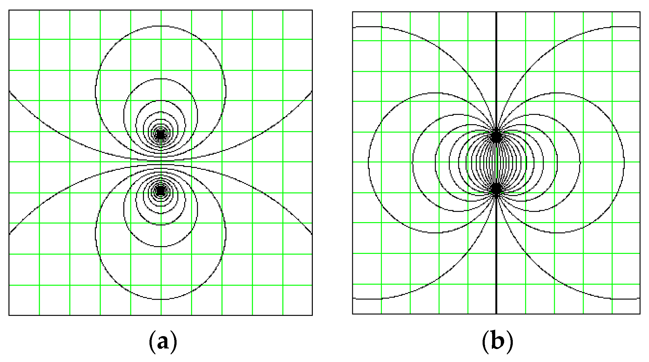
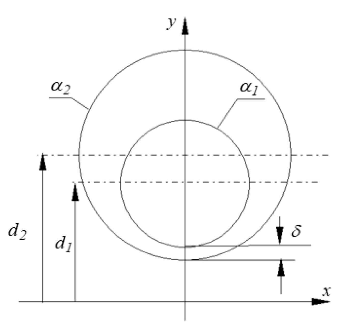
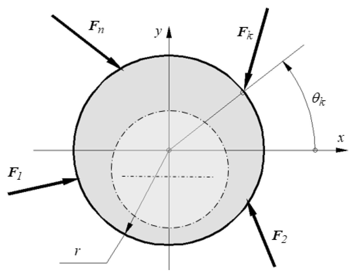
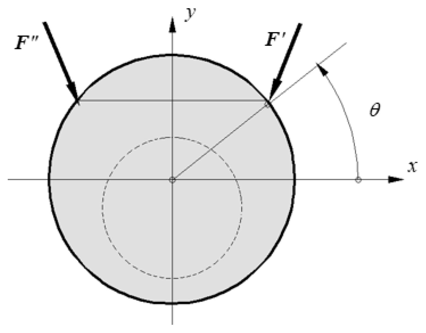
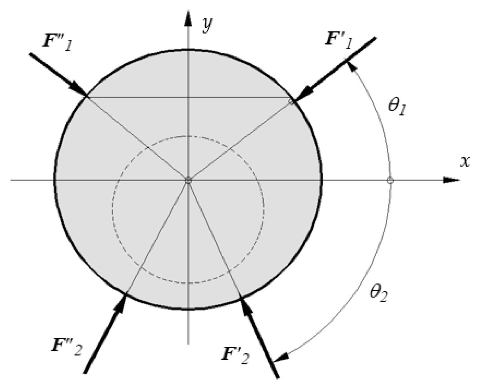
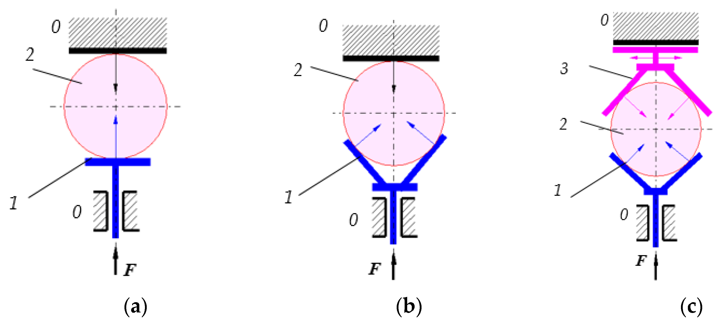
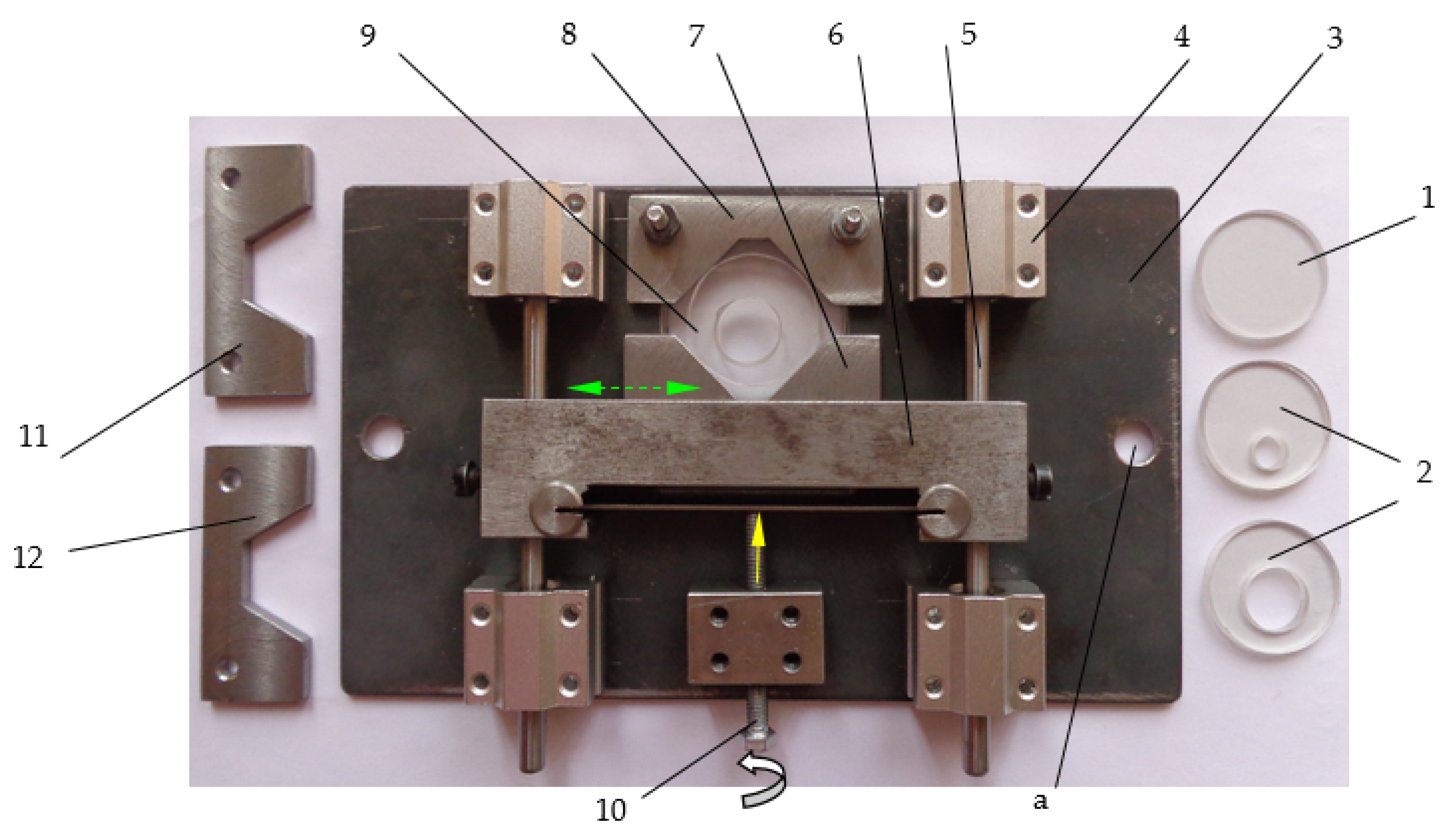
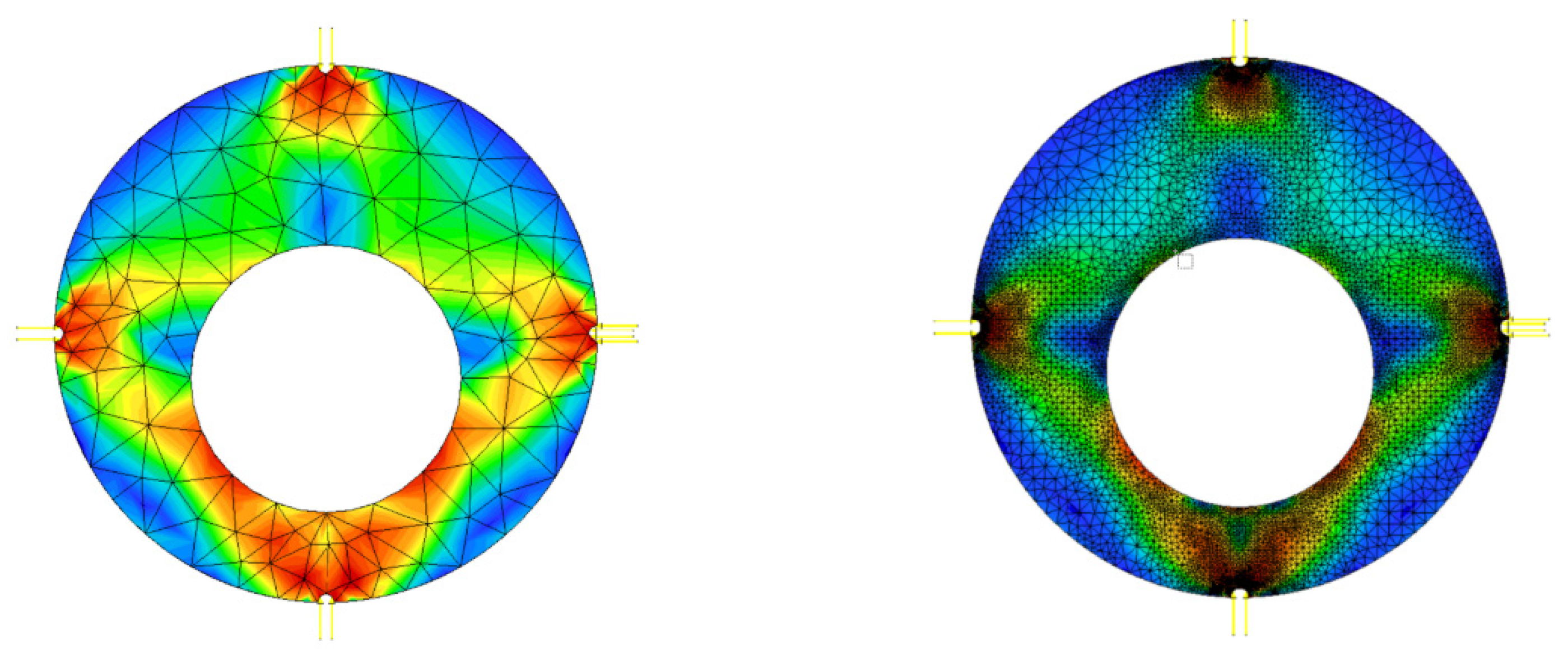
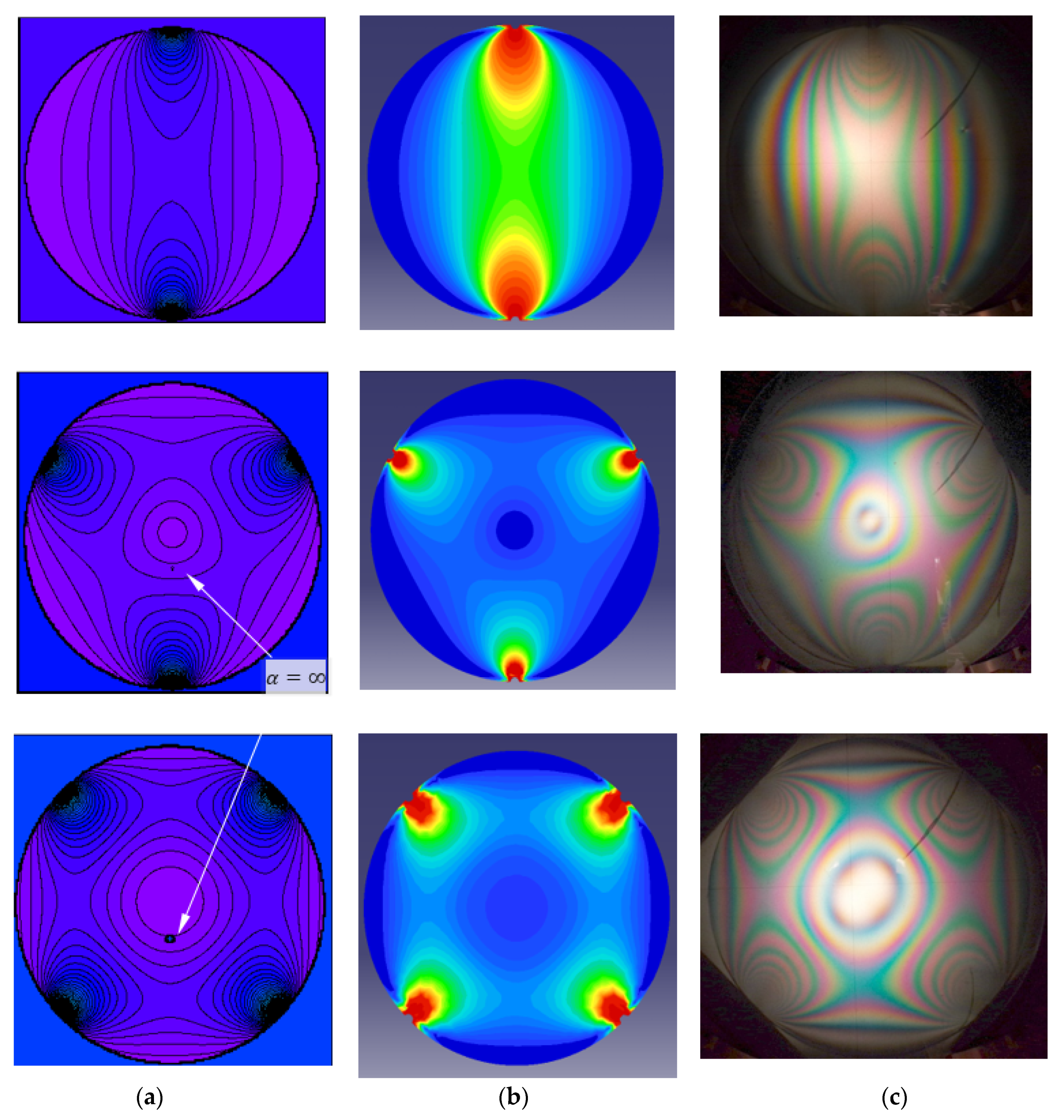
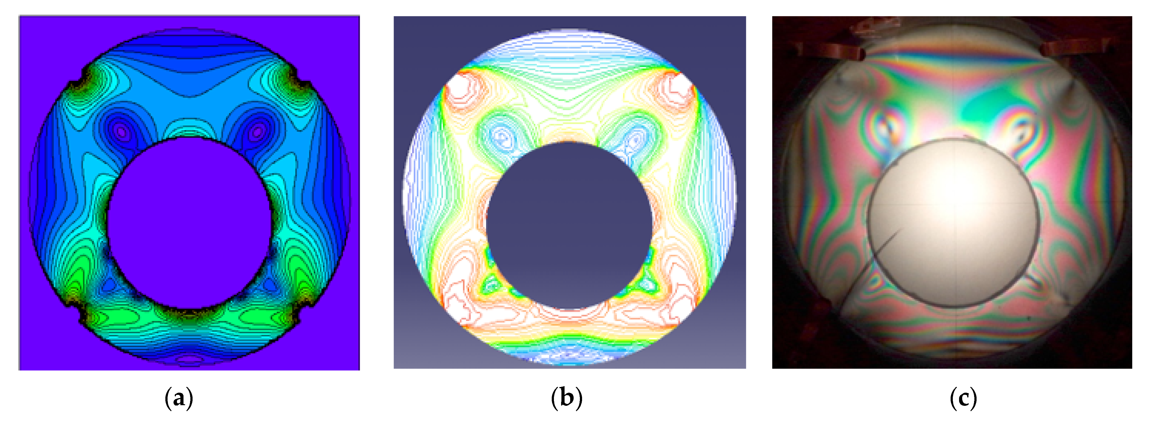
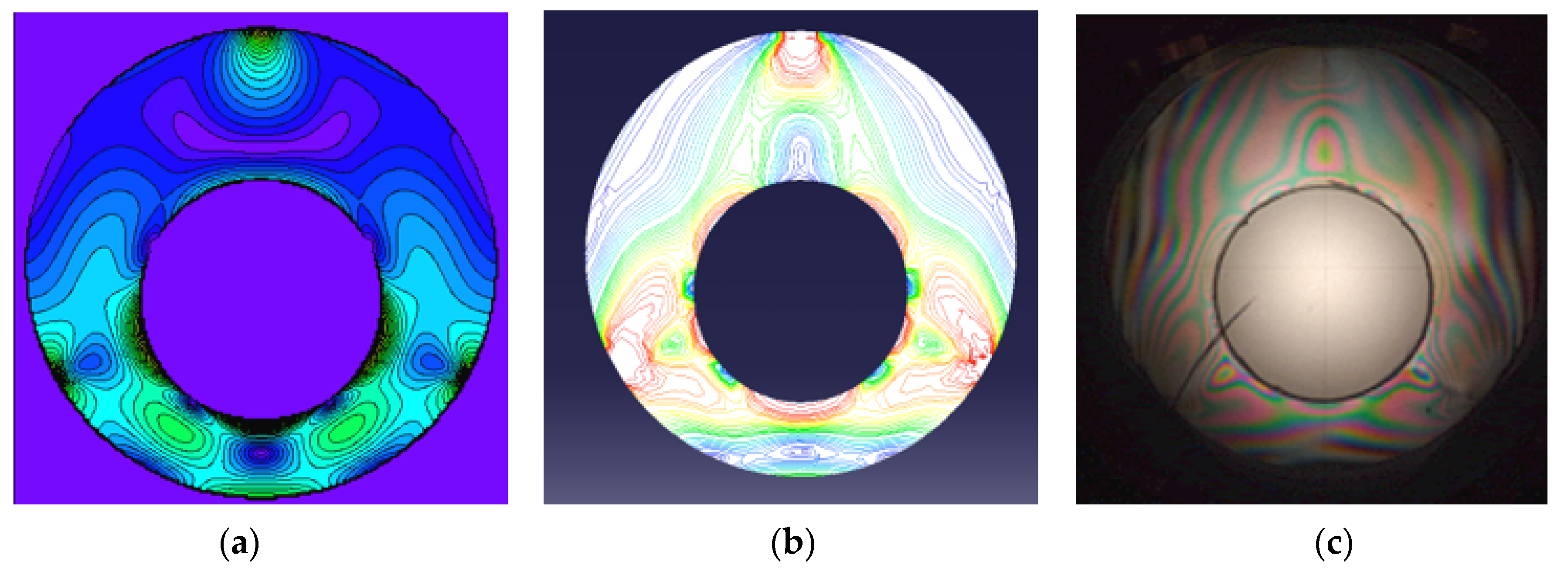
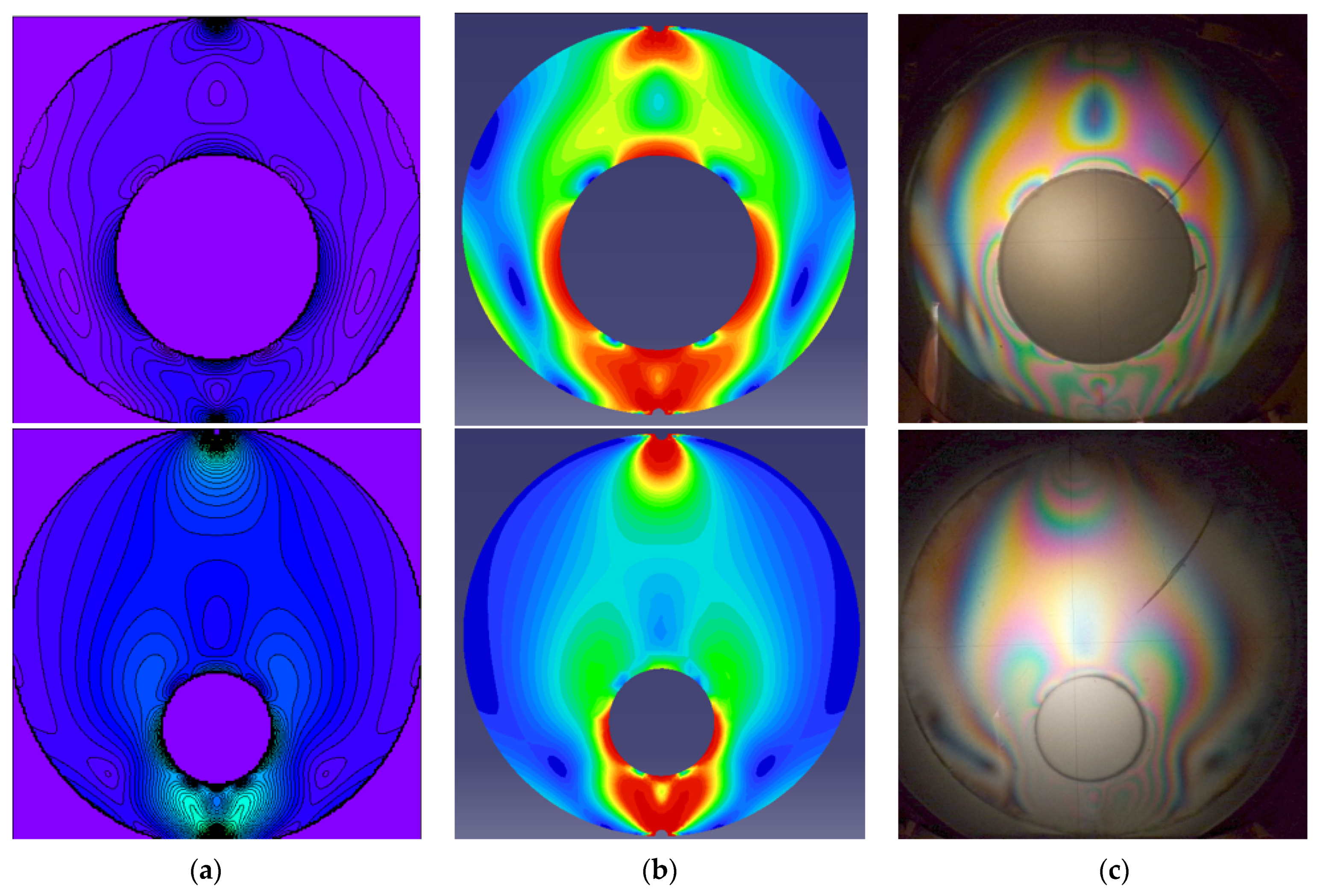
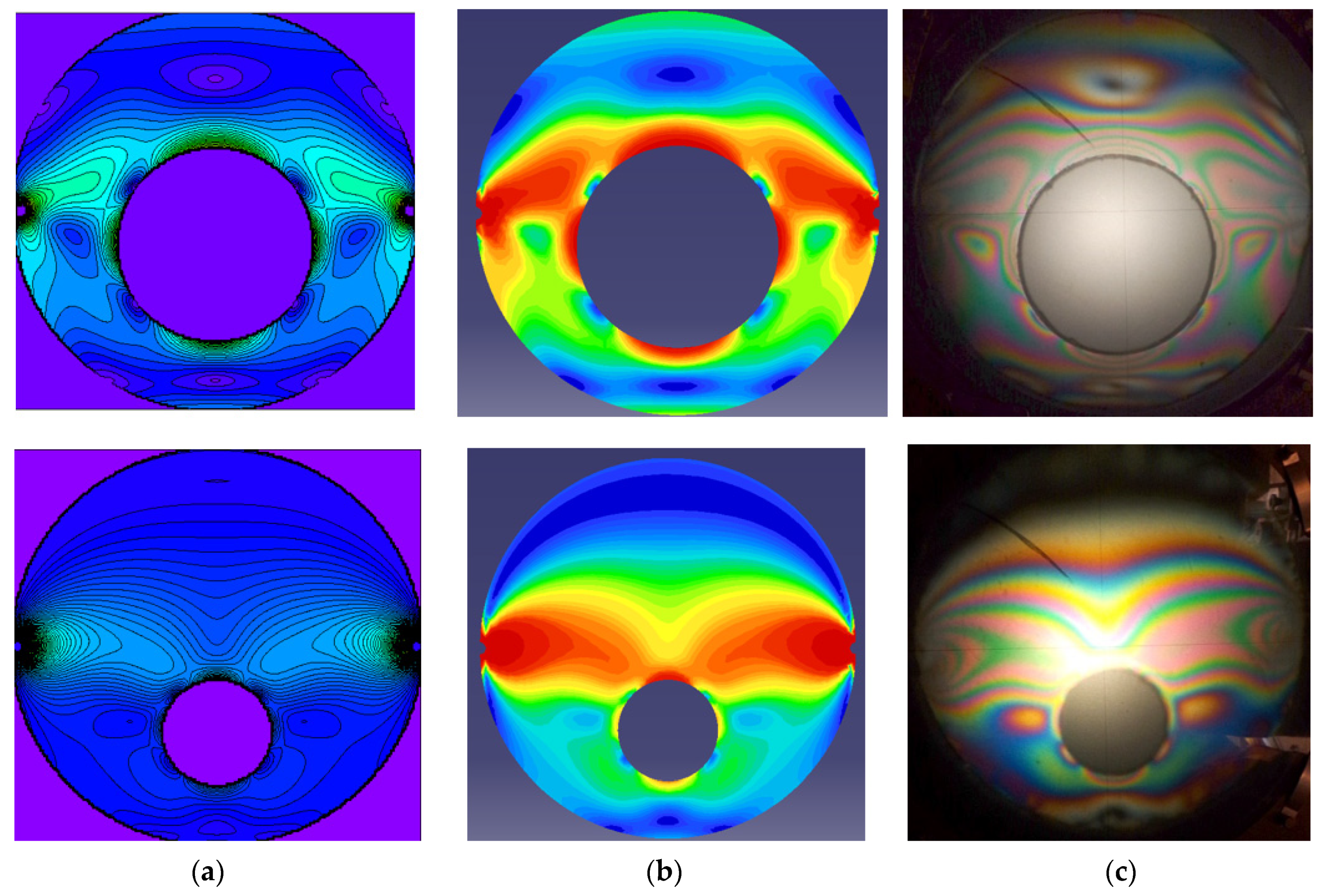
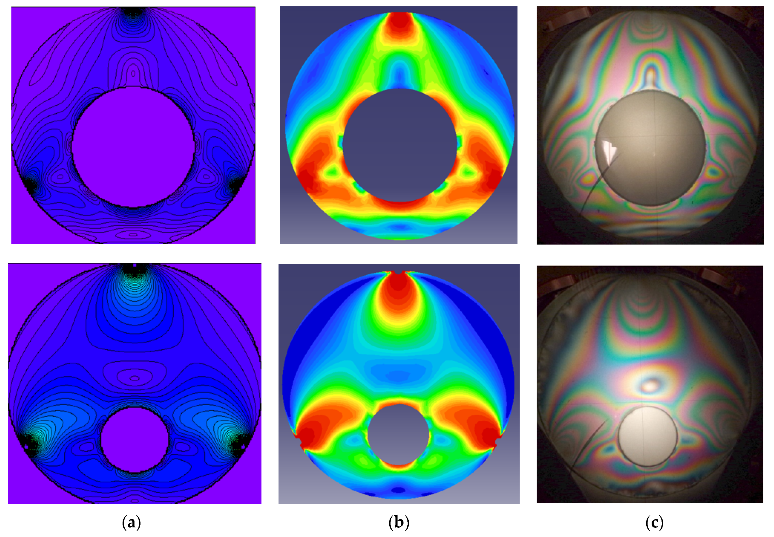
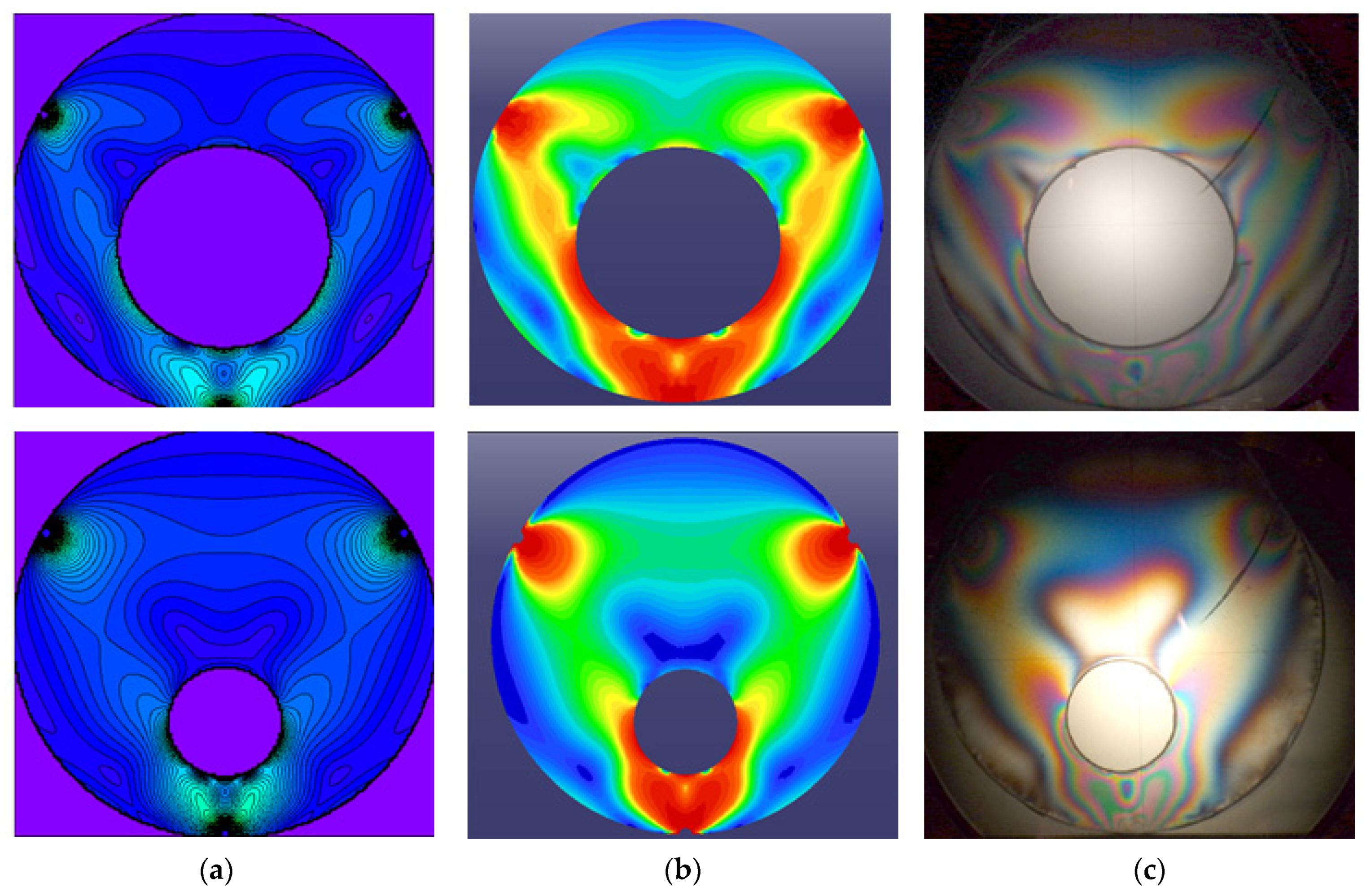
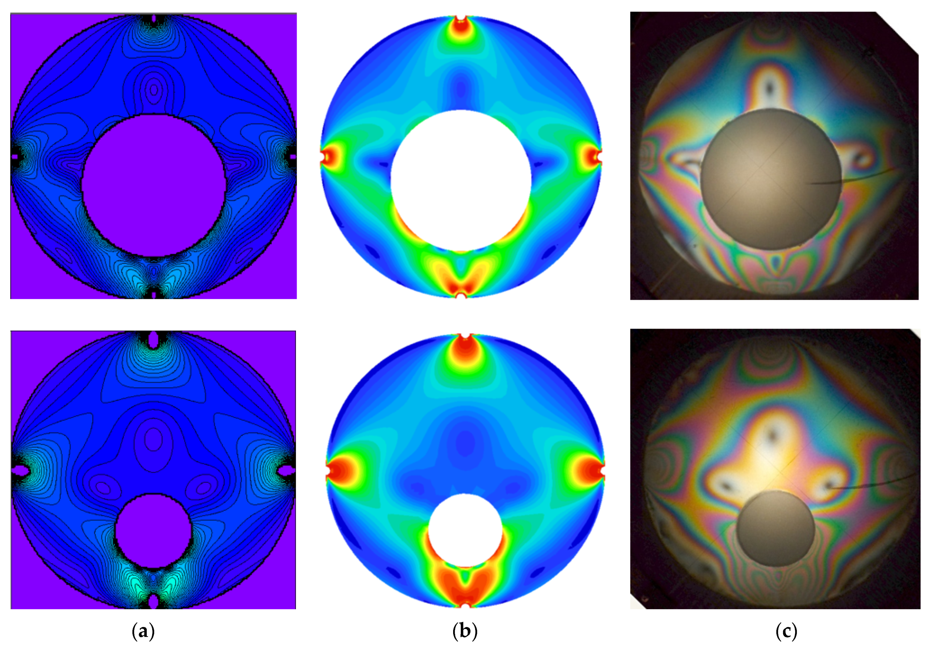
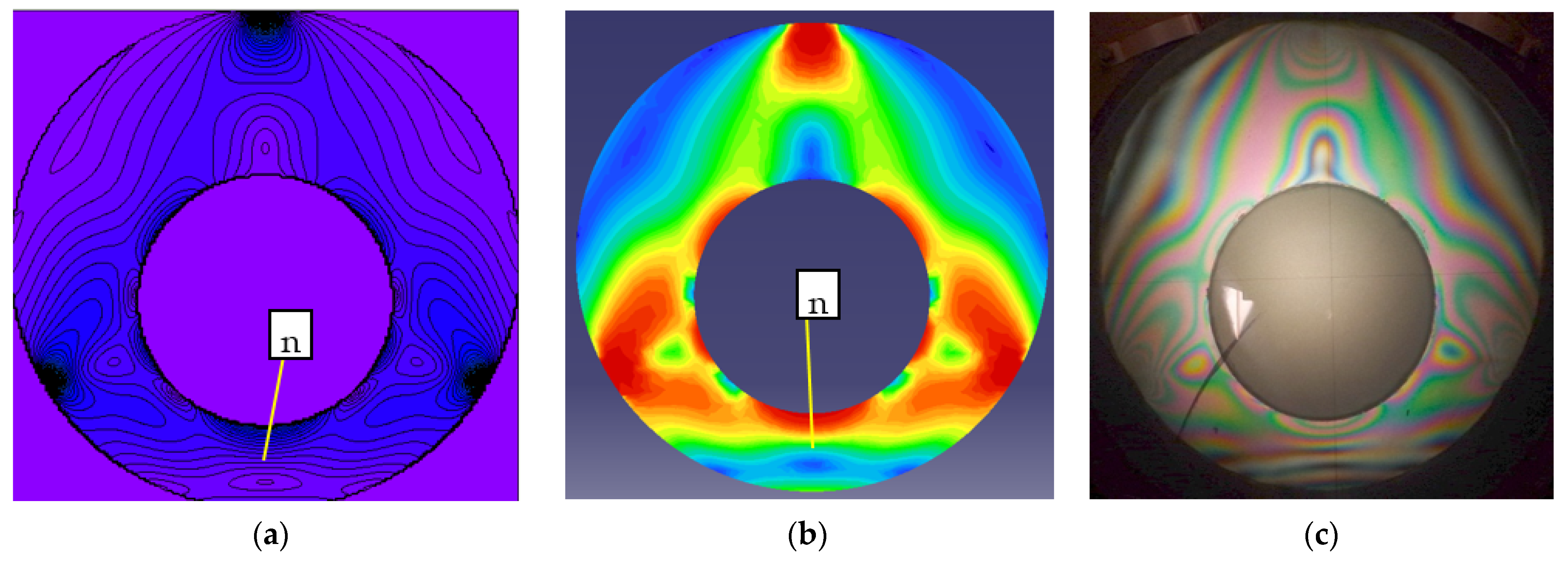
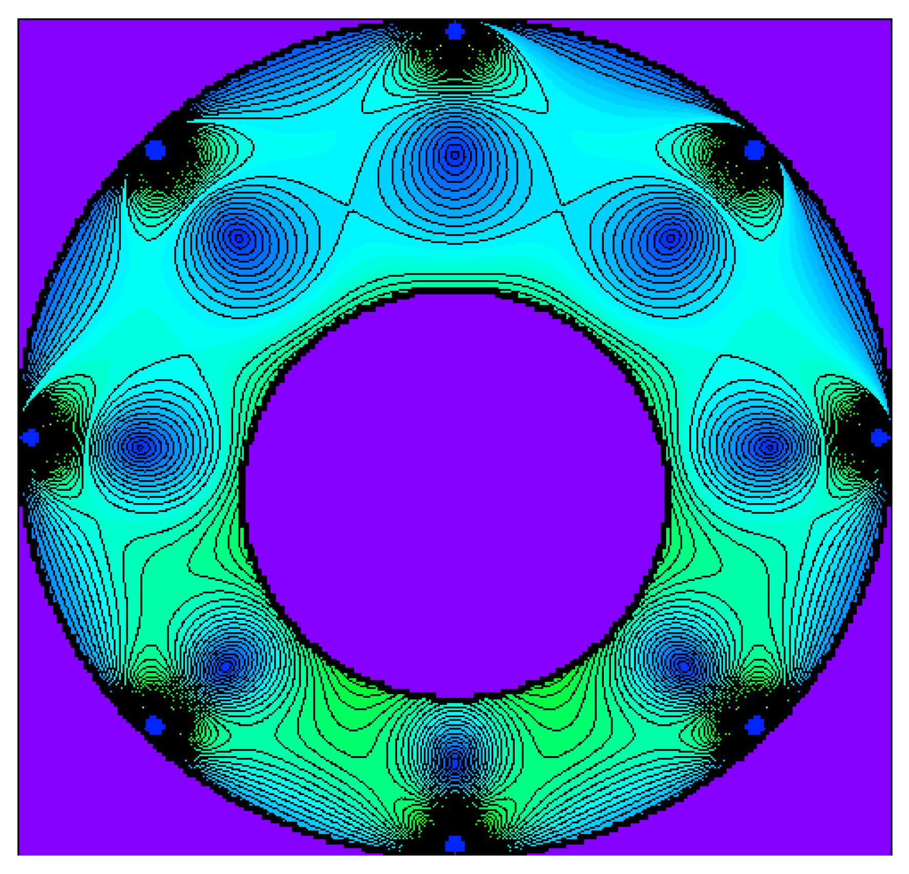
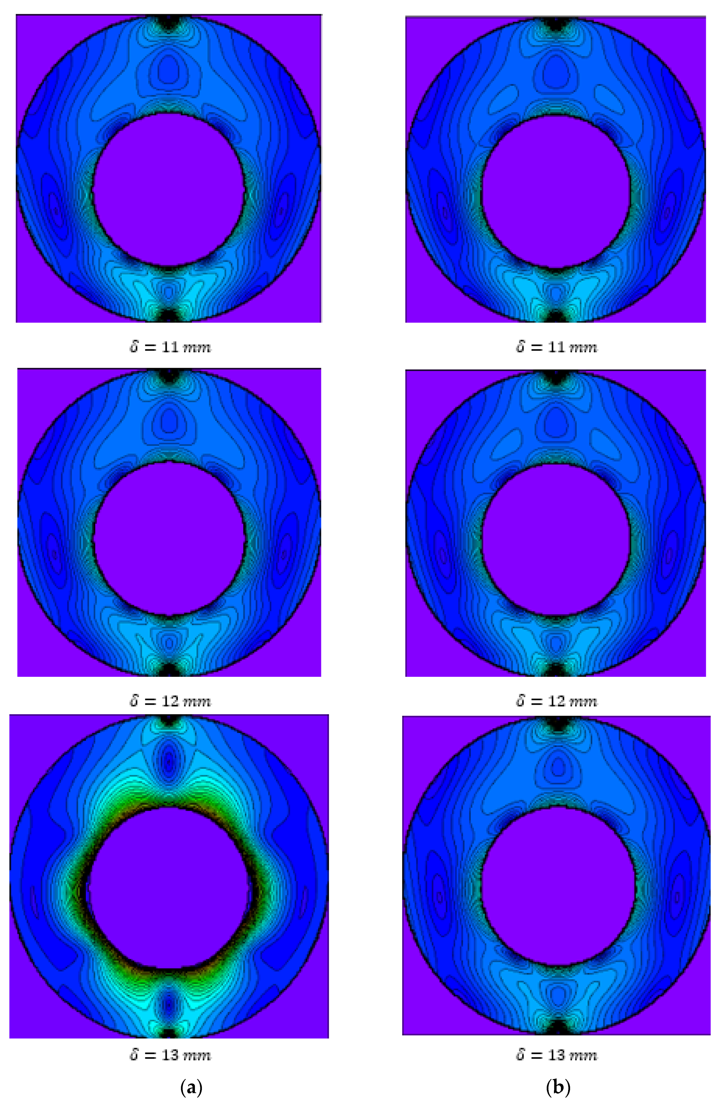
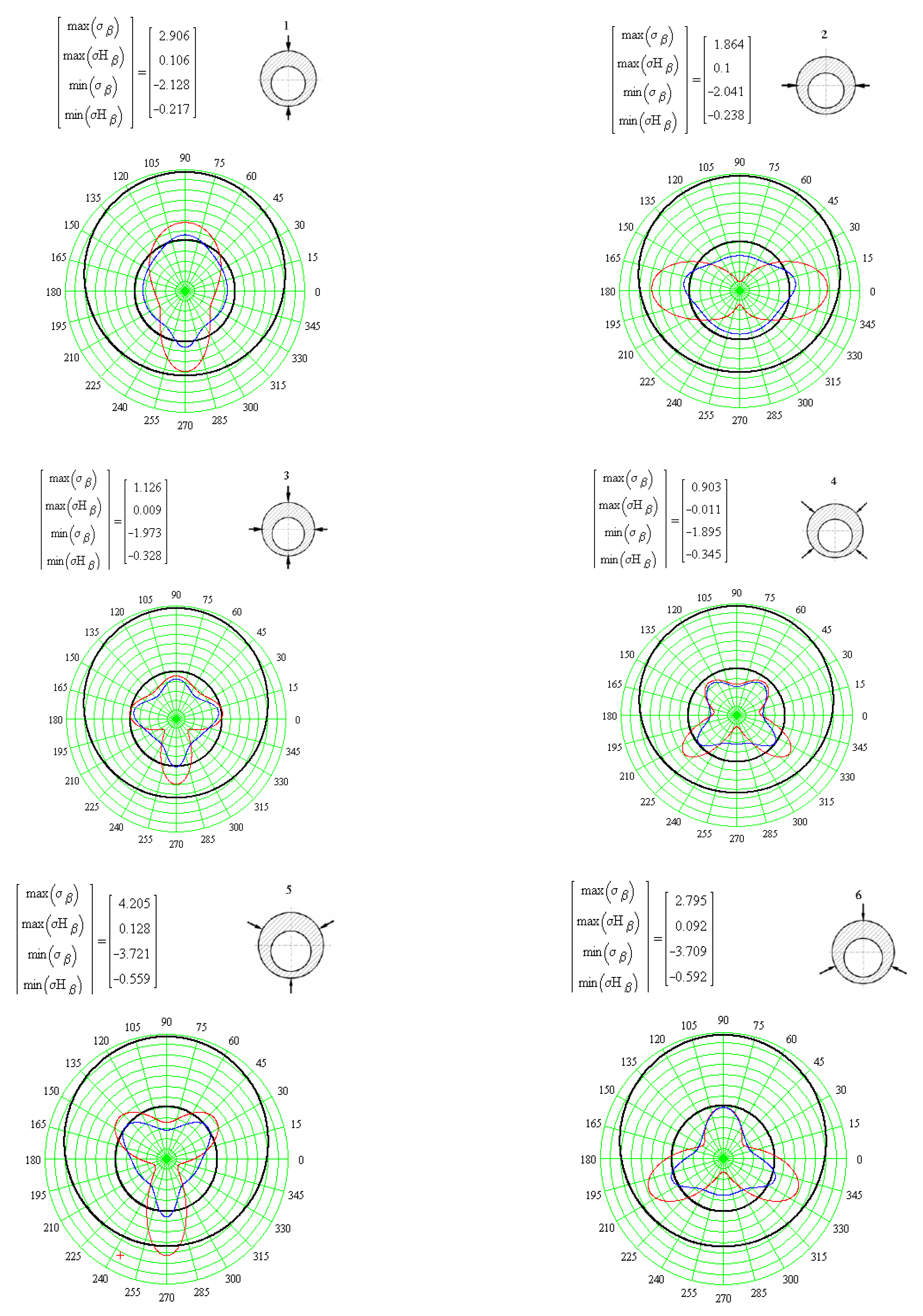
Table 1.
Symmetrical loading schematics for an eccentric ring.
| Case a | Case b | Case c | Case d | Case e | Case f | |
|---|---|---|---|---|---|---|
| Loading scheme |  |  |  |  |  |  |
| 0 |
Publisher’s Note: MDPI stays neutral with regard to jurisdictional claims in published maps and institutional affiliations. |
© 2022 by the authors. Licensee MDPI, Basel, Switzerland. This article is an open access article distributed under the terms and conditions of the Creative Commons Attribution (CC BY) license (https://creativecommons.org/licenses/by/4.0/).
Share and Cite
MDPI and ACS Style
Alaci, S.; Ciornei, F.-C.; Romanu, I.-C. Stress State in an Eccentric Elastic Ring Loaded Symmetrically by Concentrated Forces. Mathematics 2022, 10, 1314. https://doi.org/10.3390/math10081314
AMA Style
Alaci S, Ciornei F-C, Romanu I-C. Stress State in an Eccentric Elastic Ring Loaded Symmetrically by Concentrated Forces. Mathematics. 2022; 10(8):1314. https://doi.org/10.3390/math10081314
Chicago/Turabian StyleAlaci, Stelian, Florina-Carmen Ciornei, and Ionut-Cristian Romanu. 2022. "Stress State in an Eccentric Elastic Ring Loaded Symmetrically by Concentrated Forces" Mathematics 10, no. 8: 1314. https://doi.org/10.3390/math10081314
Note that from the first issue of 2016, this journal uses article numbers instead of page numbers. See further details here.