
Robust Self-Learning PID Control of an Aircraft Anti-Skid Braking System

1
School of Automation, Central South University, Changsha 410083, China
2
College of Intelligence Science and Technology, National University of Defense Technology, Changsha 410083, China
3
Laboratory of Science and Technology on Integrated Logistics Support, National University of Defense Technology, Changsha 410083, China
4
Advanced Research Center, Central South University, Changsha 410083, China
*
Author to whom correspondence should be addressed.
Mathematics 2022, 10(8), 1290; https://doi.org/10.3390/math10081290
Submission received: 18 March 2022
/
Revised: 6 April 2022
/
Accepted: 7 April 2022
/
Published: 13 April 2022
(This article belongs to the Topic Engineering Mathematics)
Abstract
:In order to deal with strong nonlinearity and external interference in the braking process, this paper proposes a robust self-learning PID algorithm based on particle swarm optimization, which does not depend on a precise mathematical model of the controlled object. The self-learning function is used to adapt to the diversity of the runway road surface friction, the particle swarm algorithm is used to optimize the rate of self-learning, and robust control is used to deal with the modeling uncertainty and external disturbance of the system. The convergence of the control strategy is proved by theoretical analysis and simulation experiments. The superiority and accuracy of the method are verified by NASA ground test results. The simulation results shows that the adverse effect of the external disturbance is suppressed, and the ideal trajectory is tracked.
Keywords:
aircraft anti-skid braking system; intelligent self-learning PID control; particle swarm optimization; robust control; uncertain disturbed systemMSC:
37M05; 37M251. Introduction to an Aircraft Anti-Skid Braking System
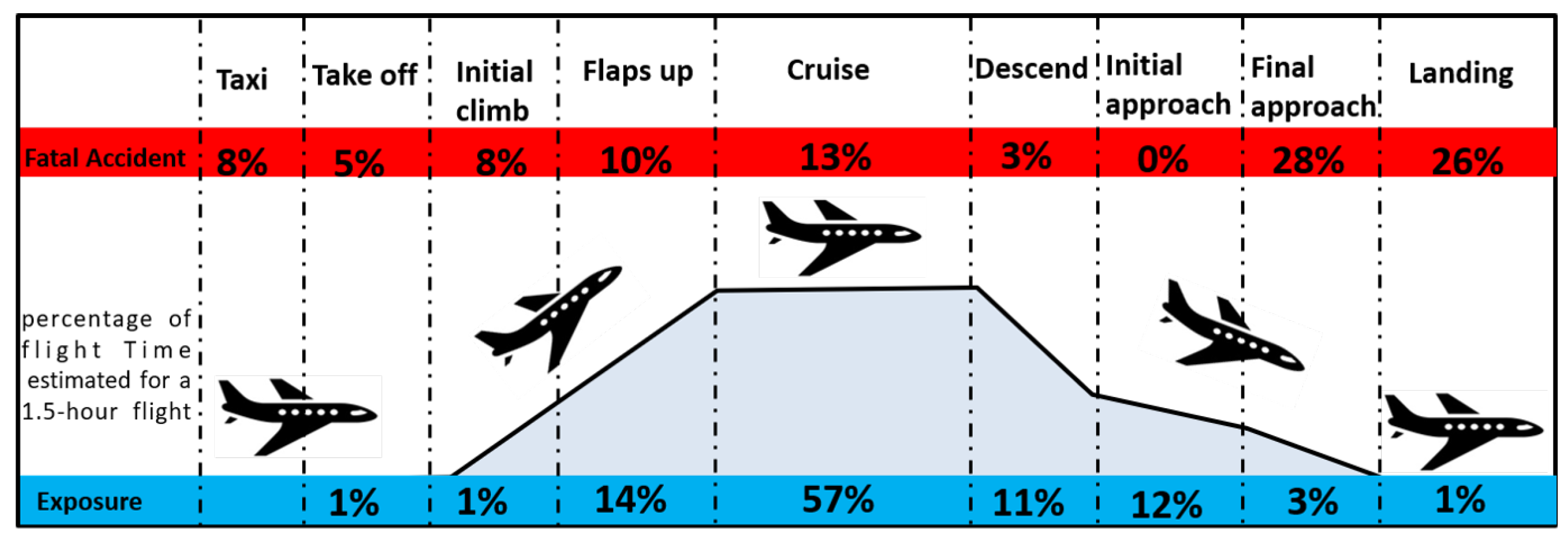
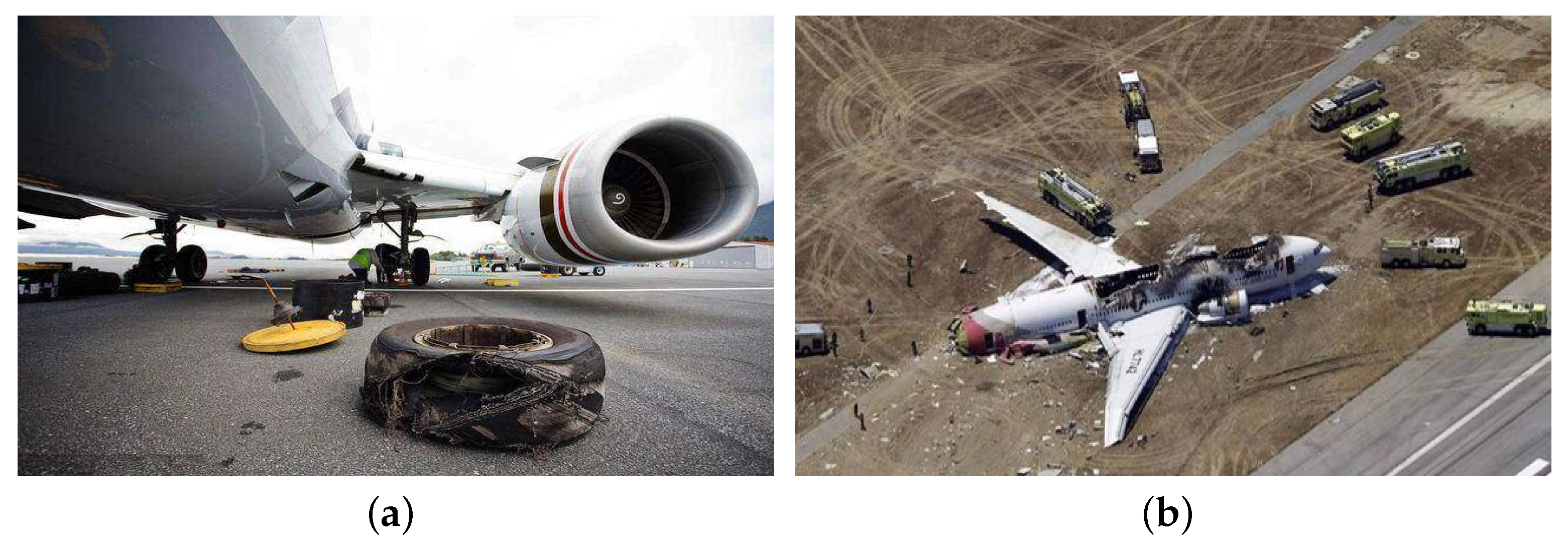
The aircraft anti-skid braking system (ABS) is important airborne equipment. Its function is to stop the aircraft in the shortest distance without skidding or self-locking. It can be seen in Figure 1 that, although the landing phase only accounts for 1% of the entire aircraft operation phase, its accident rate accounts for 26% [1]. Almost every year at home and abroad, there are aircraft accidents caused by brake system failures during takeoff or landing. Data show that the takeoff and landing stages of the aircraft are stages in the flight process with frequent safety accidents. Thus, in addition to good flight characteristics, the aircraft must also have good ground motion characteristics [2,3]. For example, on 27 June 2017, a plane at Tenerife Airport in the United Kingdom suffered a tire puncture when it landed. Some passengers were injured during the evacuation, resulting in the closure of the airport for several hours and thousands of passengers stranded at the airport. Figure 2a shows the incident. In December 2016, a domestic cargo plane ran off the runway when landing at Hangzhou Xiaoshan Airport, as shown in Figure 2b. The front fuselage of the plane was damaged, and some passengers were injured. Later, it was determined that the accident occurred because the runway was slippery, and the brake anti-skid control system did not work properly. It can be seen that the performance of the aircraft braking system directly affects the safety of the aircraft and the people on board. It is required that the brake anti-skid control system must work stably, quickly, and accurately to ensure the safety of the aircraft.
The aircraft anti-skid braking system (ABS) was designed to maximize the friction between the tires and the road surface by controlling braking pressure in real time, thereby improving the braking efficiency and shortening the braking distance [4]. The early anti-skid braking control algorithm of an aircraft was inertial anti-skid, which realized an anti-skid operation by setting a threshold value for the wheel speed deceleration rate. In order to deal with the unwanted impact of the estimated accuracy of automotive reference speed on logic threshold control, aircraft reference speed was estimated using a correctional peak–to–peak connection method, and a mixed slip rate and acceleration threshold control was proposed [5]. However, it was difficult to design this kind of controller, as the performance of this kind of method heavily depended on parameters to be determined by engineering experience, and it was also difficult to evaluate the stability of such a controller. In recent years, a slip-rate-based control algorithm has become the focus of the ABS for the improved braking efficiency of this kind of control strategy. With the slip rate concept introduced into the anti-skid control, the controller can control the slip rate operating near the optimal value, so as to make full use of the friction between the road surface and the tire, thus improving the braking efficiency and shortening the braking distance. Many scholars have devoted themselves to researching the slip-rate-based control of the ABS, and have proposed many high-performance anti-skid control algorithms, such as fuzzy control [6,7], sliding mode control [8,9], switching control, and neural network control [10,11].
Based on regenerative, kinetic, and short-circuit braking mechanisms, a novel method of realizing an anti-skid braking system (ABS) controller was proposed in [12]. In the paper, a boundary layer speed control was used to guarantee the optimal track of the slip rate between the tires and the road surface, and the braking performance of the controller was addressed via real-world experiments. In [13], sliding mode control approaches were proposed to realize the slip control of the vehicle, which can make the wheel slip rate follow a desired value, while guaranteeing that the sliding mode control is stabilizing. Many model-based control algorithms have been proposed, such as optimal control [14,15], sliding-mode control [16,17,18], fractional order sliding-mode control [19,20], gray sliding-mode control [21], and feedback linearization control [22]. To better design a model-based controller, a full-order dynamic model must be provided, which is fairly difficult for a system such as an aircraft anti-skid braking system.
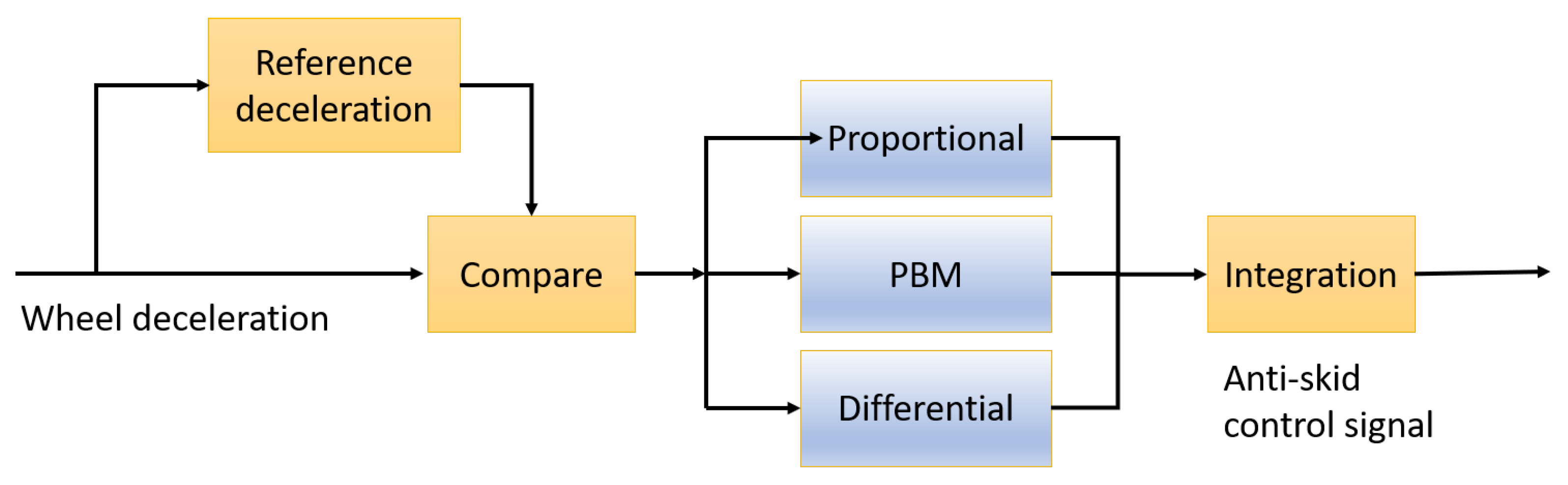
For a strong real-time and highly nonlinear system such as ABS, the unmodeled dynamics and parametric uncertainty may lead to serious performance degradation [23]. Therefore, model-free control technology has gradually attracted the attention of anti-skid system researchers. The model-free control techniques are also labeled as data-driven [24], because a large amount of test data is needed to design the controller. Currently, a pressure-bias-modulated (PBM) aircraft anti-skid braking system is the most commonly used braking system, which is an improved algorithm of PID control. Figure 3 is a schematic diagram of a slip-velocity-controlled, PBM control system, which demonstrates that the only difference between the PBM and PID control algorithms is that the integration module of a PID algorithm is replaced by a PBM module algorithm. It retains the advantages of a simple and easy-to-understand PID controller and does not require an accurate system model of the controlled object. Although a large number of new anti-skid control algorithms have emerged in recent years, it is still the most widely used and installed anti-skid control algorithm.
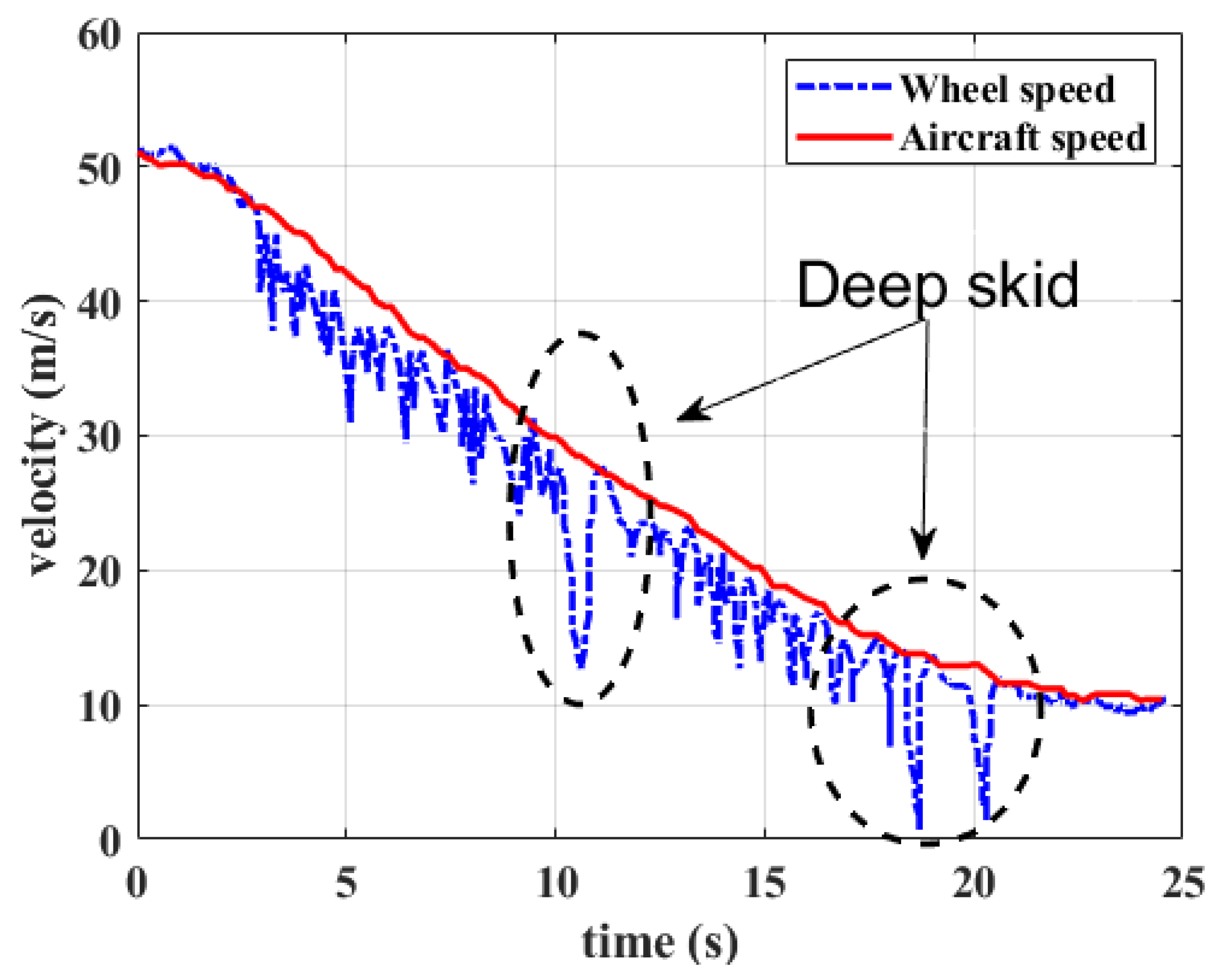
Although the PBM algorithm has a good braking effect under dry runway conditions, when the runway is slippery or icy, it is prone to deep slippage, resulting in low braking efficiency. Figure 4 is the curve of the PBM controller slipping on a slippery runway [25]. A deep skid not only accelerates tire wear and reduces tire life but also easily causes the aircraft to overrun the runway with a braking distance that is too long.
In summary, although many new intelligent anti-skid braking algorithms have emerged in the academic world, albeit limited by the computing power of the aircraft chip, there is still a need for simple and easy-to-implement anti-skid controllers, such as PID algorithms and their improved forms. Motivated by this, in this paper, we propose a robust self-learning PID controller for optimum slip rate tracking during the aircraft braking process.
2. ABS Dynamics and Control Problem
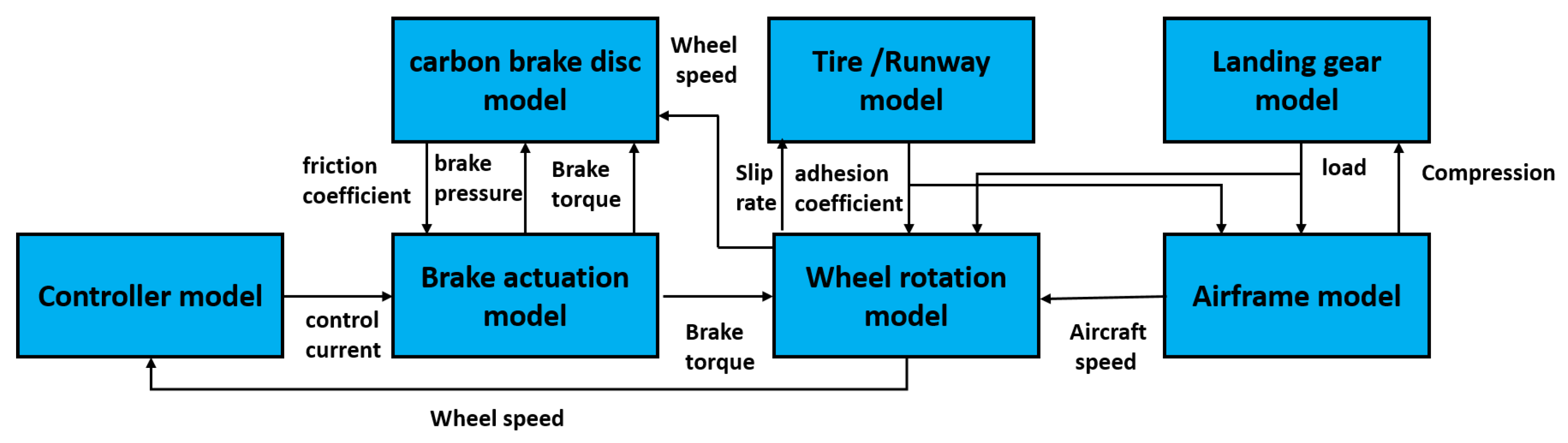
Aircraft brake ground test costs are high and the experimental period is long; so, the design of an aircraft anti-skid braking system usually uses computer simulation to assist the design. Similar to an actual aircraft, the aircraft model used for simulation is also an assembly of many unique subsystems. The relationship between the aircraft braking system dynamics model and the controller model is shown in Figure 5.
2.1. Aircraft Dynamics during the Braking Process
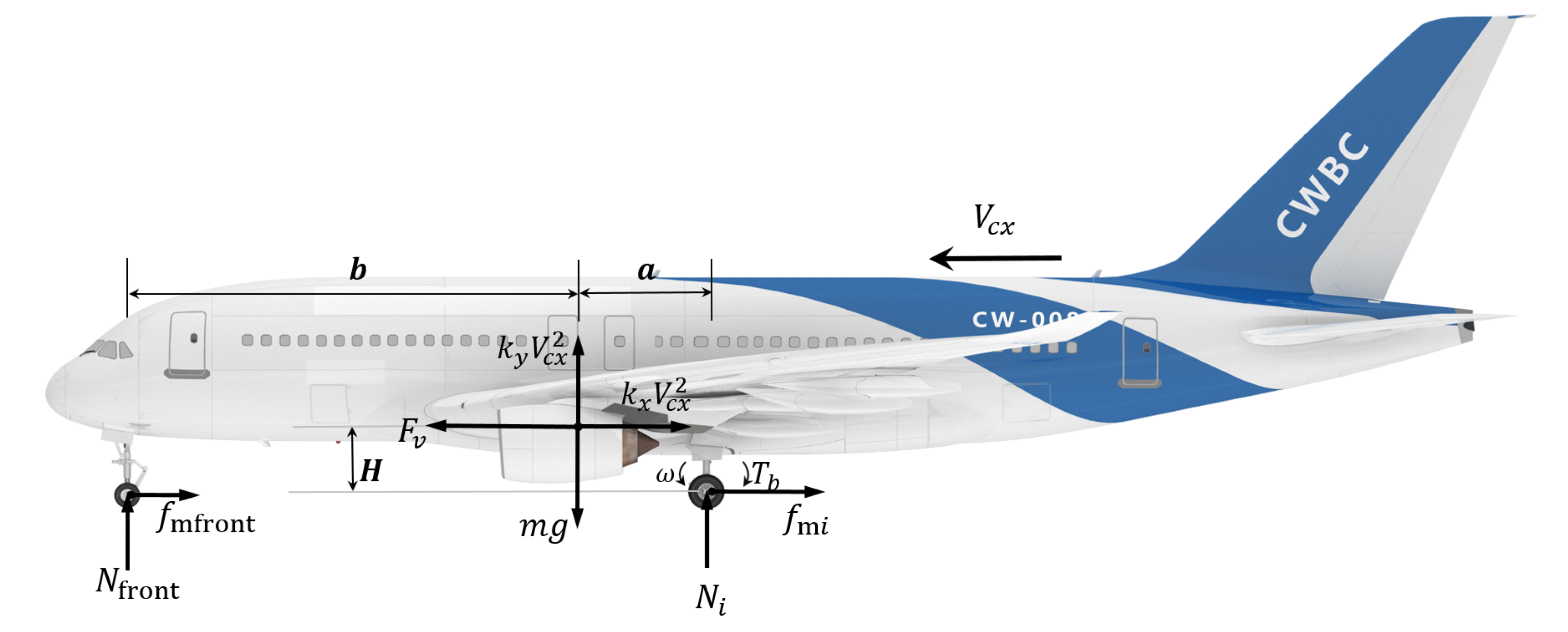
In the process of landing braking, the aircraft is mainly affected by the supporting force of the tire and the landing gear, the friction between the road surface and the tire, and the friction between the air resistance and the lift. A schematic diagram of the aircraft force is shown in Figure 6.
The dynamics of the aircraft during braking can be formulated as
where , , , and .
The parameters of the aircraft ABS are illustrated in Table 1.
The deceleration of the aircraft mainly depends on the friction between the main wheel and the ground, and the relationship can be given as
Therefore, the dynamic model of the aircraft fuselage can be characterized as
2.2. Dynamics of Wheel and Tire
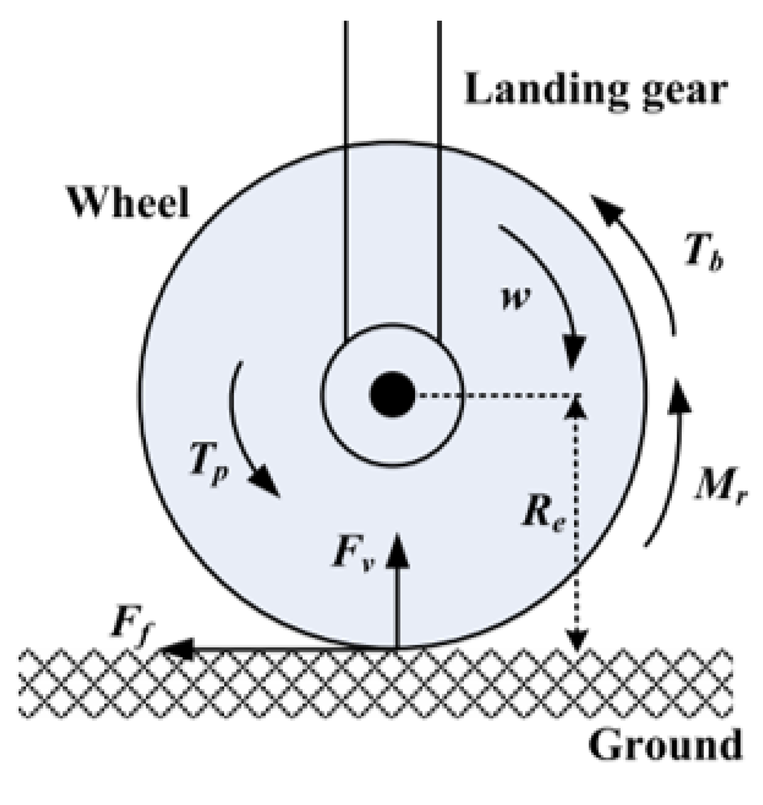
Figure 7 is a schematic diagram of the main wheel of the aircraft, from which we can see that the wheel is mainly subjected to the ground support force, braking force, and the ground friction during the braking process. The rotational dynamics of the main wheel can be described by
where is the moment of inertia of the braking wheel, and is the effective rolling radius of the braking wheel. is the brake torque generated by the actuator.
In order to describe the slip state of the braked wheel, a new variable slip rate is proposed. The slip rate of ABS is defined as follows:
During braking, the slip rate ranges from 0 to 1, with representing free rolling, and representing tire lock. Taking the derivation of yields
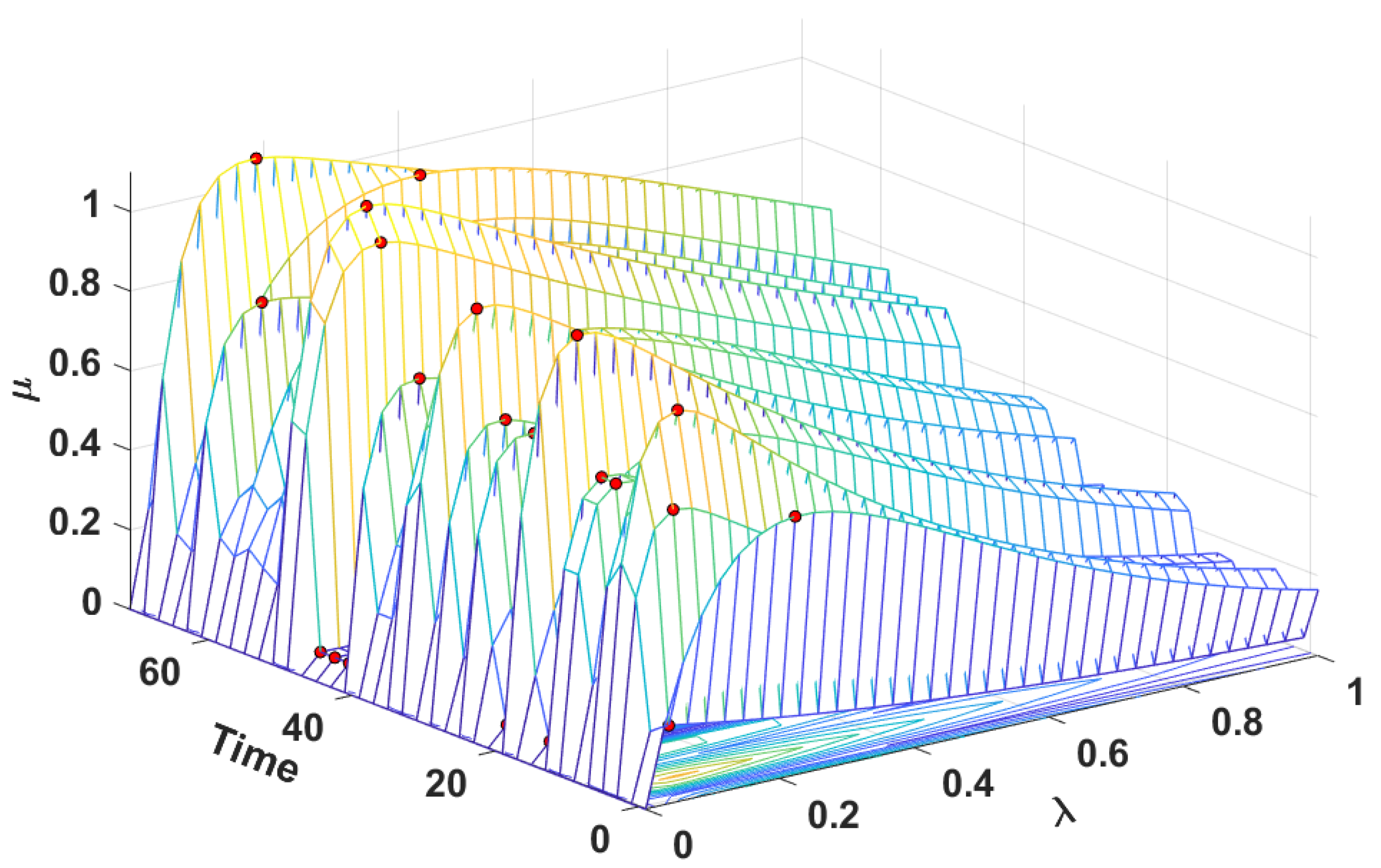
From Equation (4), it can be seen that the friction between the tire and the ground is related to the load in the vertical direction of the tire and the road surface adhesion coefficient. In this paper, the friction model proposed by Burckhardt [26,27] is adopted, and the parameters of the tire model are shown in Table 2.
The friction characteristics under different runway conditions and the optimal slip rate corresponding to the system are shown in Figure 8, the red dots represent the optimal slip rate values on different runways.
2.3. Brake Actuator Dynamics
During the braking process, the function of the brake actuator is to convert the current output by the braking system into the corresponding braking force. During the braking process, the torque of the brake actuator is applied to the brake device mounted on wheels. The dynamics of the actuator can be expressed by the following equations:
2.4. Overall Dynamics of the Aircraft Anti-Skid Braking Process
For anti-skid braking control, the variable we are most concerned with is the slip rate of the system, and according to its definition, it is related to the speed of the body and the linear speed of the braked wheel; so, in order to obtain the slip rate dynamic characteristics, Equation (6) is substituted into Equations (1) and (3) to calculate and . We then obtain
From the above equations, we observe that the aircraft speed is not directly controlled by Tb. However, the wheel slip rate can be controlled by Tb, i.e., depending on and . Taking the time derivative of Equation (7), we obtain
Therefore, considering the actuator dynamics, the overall aircraft braking model can be rewritten as
The aircraft landing braking system has strong nonlinearity and model uncertainty, which can be seen from the above equation. There are two main sources of nonlinearity and uncertainty. The first factor is the nonlinear relationship between the wheel slip rate and the longitudinal speed of the wheel . In addition, the measurement of the aircraft speed usually has errors. All of these characteristics make the design of an ABS control law difficult [28].
3. Problem Formulation
According to the above formula, we can see that, in order to improve the braking performance of the aircraft ABS, the anti-skid control system needs to track the optimal slip rate signal. It is well known that when the system is at the optimum slip rate value, the bonding force between the tire and the ground is the largest, and the aircraft braking efficiency is the highest. The optimum slip rate will vary due to changes in runway conditions, aircraft speed, wheel speed, etc. However, most of the existing ABSs are designed to track a constant value set in advance based on engineering experience, rather than the real-time optimal slip rate [28,29,30]. To simplify the controller design process, without a loss of generality, the controller design adheres to the following assumptions:
- The aircraft should maintain a straight taxiing direction.
- The fuselage and landing gear are ideal rigid bodies. The aircraft fuselage has no vertical and pitch displacement.
- The vertical load is evenly distributed, and the friction between the left and right wheels is symmetrical.
To facilitate the controller design, let , and , i.e.,
The expression of aircraft dynamics can then change to the following form:
where is the derivative of the aircraft longitudinal acceleration, and by neglecting unmodeled dynamics and external disturbance, System (17) can be rewritten as
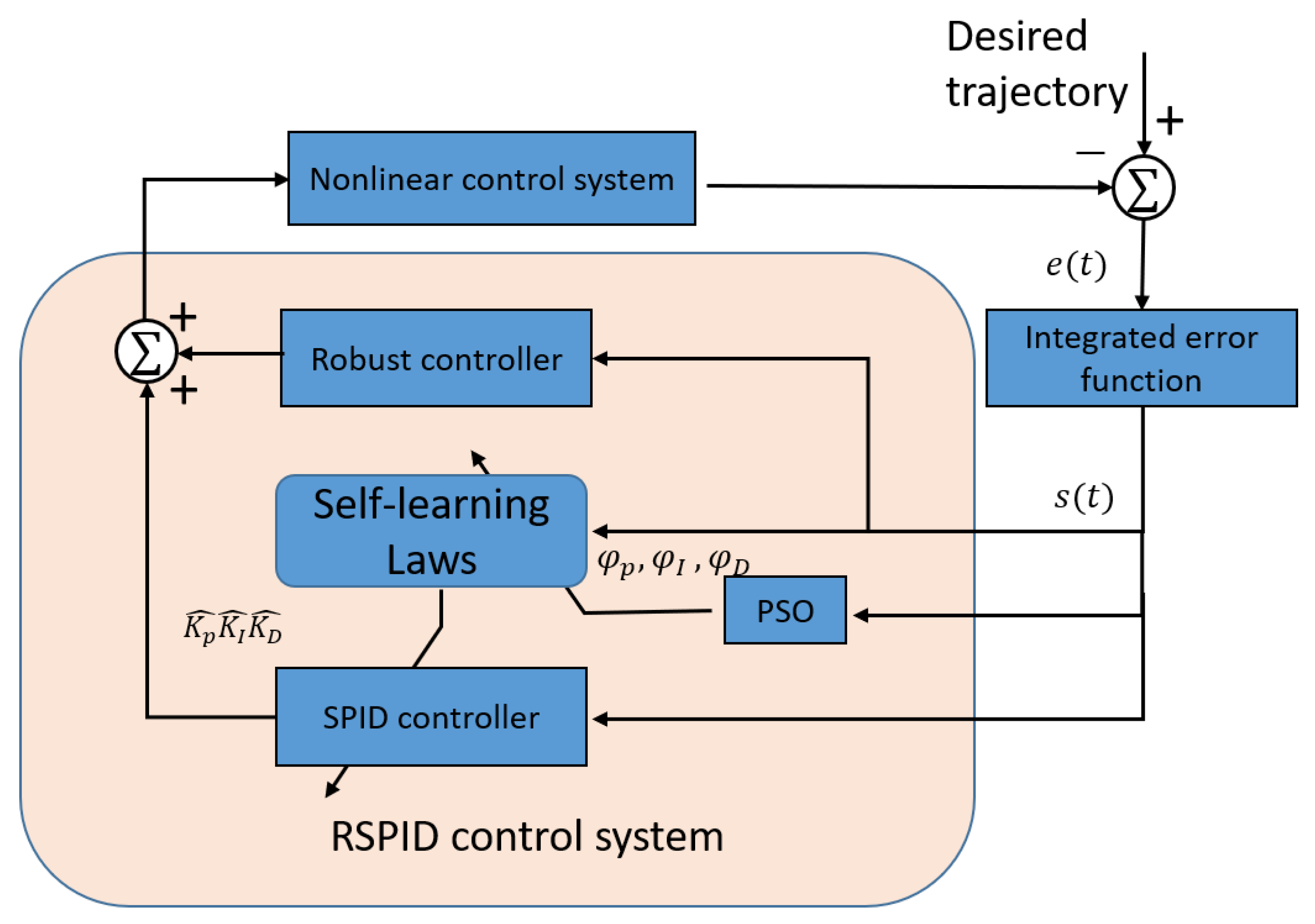
4. Robust Self-Learning PID (RSPID) Control System Design
According to Equation (19), the design of an anti-skid control system is to find a suitable algorithm under which the output of the system can track optimal trajectory closely [32].
In order to design the control algorithm, the tracking error is defined as
Therefore, the error vector of the system can be expressed as
If the uncertainty of the system and external disturbances can be accurately obtained, then an ideal controller can be designed as
where is the feedback gain matrix. We can then obtain a dynamic system error equation by substituting Equation (21) into Equation (17):
If the Hurwitz polynomial is used to generate the corresponding coefficients in the H matrix, it means that . However, in the design of the actual controller, the uncertainty, nonlinearity, and external disturbance of the system are usually unknown and unpredictable, which makes the ideal controller (22) unobtainable. Therefore, the SPID controller is adopted to simulate the output of the ideal controller, and a robust controller based on the method is then designed to compensate for the track error between the SPID controller and the ideal controller, thereby improving the robustness of the system. The RSPID control system is assumed to take the following form:
where is the output of the SPID controller, and is the output of the robust controller designed to suppress the influence of the residual error between the SPID controller and the ideal controller. The block diagram of the nonlinear control system is shown in Figure 9.
4.1. The Design of an SPID Controller
The expression of the SPID controller can be described as
where (proportional gain), (integral gain), and (derivative gain) are the adaptive tuning parameters of the proposed controller.
The system integrated error function is then defined as
where .
The control law Equation (23) can then be rewritten as
By defining as a cost function, its derivative is . According to the gradient descent method, the gains of , and are updated by the following tuning laws:
where is the output value of at the ith time, and , , and are the learning rates, which are determined by the PSO algorithm in real time.
4.2. The Design of the Robust Controller
Because of the model uncertainty and outside disturbance, there is always a tracking error between the output of the controller and the output of the ideal controller, and the error can be expressed by the following expression:
Equation (23) can be converted into the following form:
In case of the existence of , a specified tracking performance is considered [33]:
where is a prescribed attenuation constant. The robust controller is designed as
where .
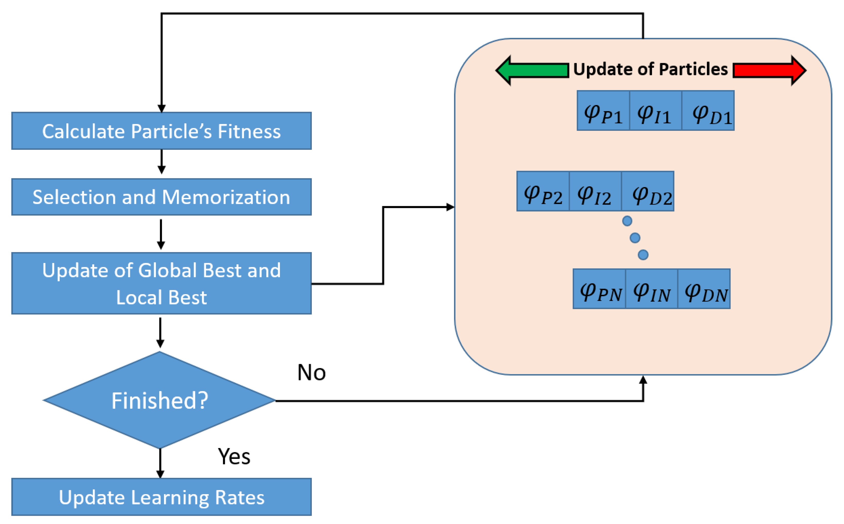
4.3. The Design of the Particle Swarm Optimization Algorithm
The concept of a PSO algorithm was initially proposed by Kennedy and Eberhart [34] in 1995, and it has been shown to be effective in solving optimization problems [35]. According to Kennedy and Eberhart, each particle represents a candidate solution to the optimization problem. Each particle tracks the optimal solution by moving its position; acceleration is weighted by a random term where separate random numbers are generated for acceleration towards the local best and global best positions [36]. In order to achieve a better learning speed and spare the trial and error process of selecting a suitable learning rate, the particle swarm optimization (PSO) algorithm is used to track the optimal learning rates in real time. The flowchart of the PSO used to adjust the learning rate is shown in Figure 10. In this paper, the particle swarm algorithm is used to find the optimal learning rate of the PID algorithm; so, we chose the learning rate as the coordinate of the example. The optimization goal is to track the optimal slip rate of the system. Thus, the fitness function is constructed using the tracking error between the actual slip rate and the optimal slip rate. The fitness function was chosen as follows:
This means that the fitness value ranges from 0 to 1; the larger the fitness value, the better the optimization effect.
The velocity and position update law of particles is adopted as
5. Simulation Results and Discussion
In order to verify the control scheme proposed in this paper, this study builds an aircraft anti-skid brake model on the Matlab/Simulink platform. The model used is shown in Figure 11.
The simulation model is mainly composed of several submodules: a fuselage dynamics module, a tire and ground friction module, a controller module, and a brake device module. The airframe dynamics module is mainly used to simulate the dynamic characteristics of Equations (1)–(3). Its main input is the braking torque information output by the braking device, and its main output is the aircraft pitch angle, speed, and other information. The tire ground friction module mainly simulates the dynamic characteristics of the wheel described by Equations (6)–(9). Its main input information is aircraft body speed, pitch angle, and other information, and its output is information such as the ground friction force and the system slip rate. The controller module mainly simulates the robust self-learning algorithm proposed in this paper. The main input variable is the system slip rate, and the main output is the anti-skid current. The anti-skid current is converted into the braking torque through the braking device module, and then transmitted to the airframe dynamics module.
5.1. Model Verification
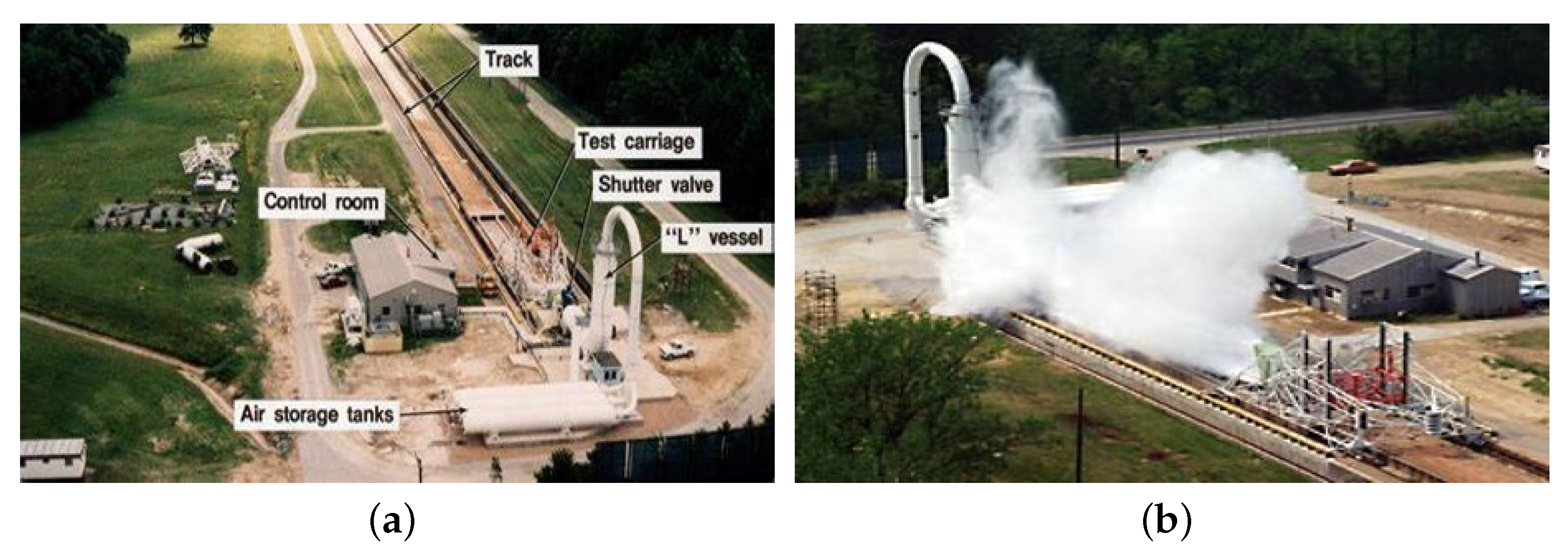
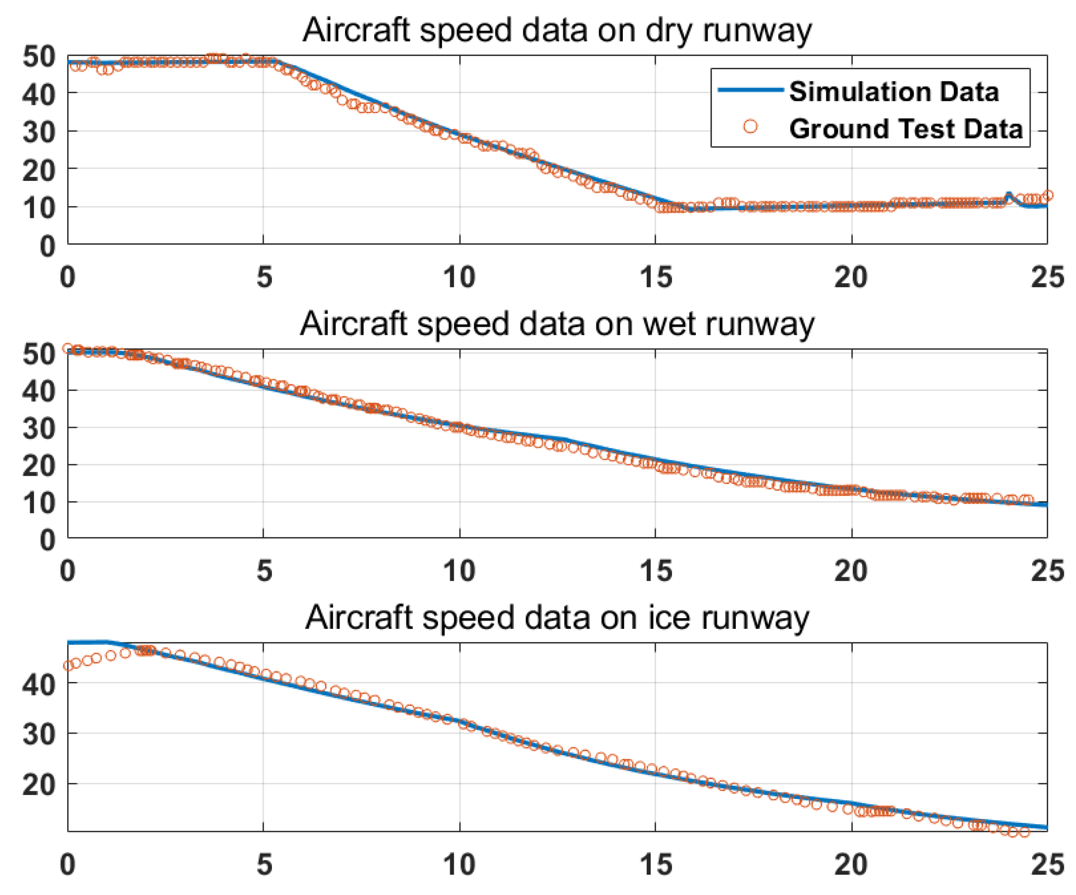
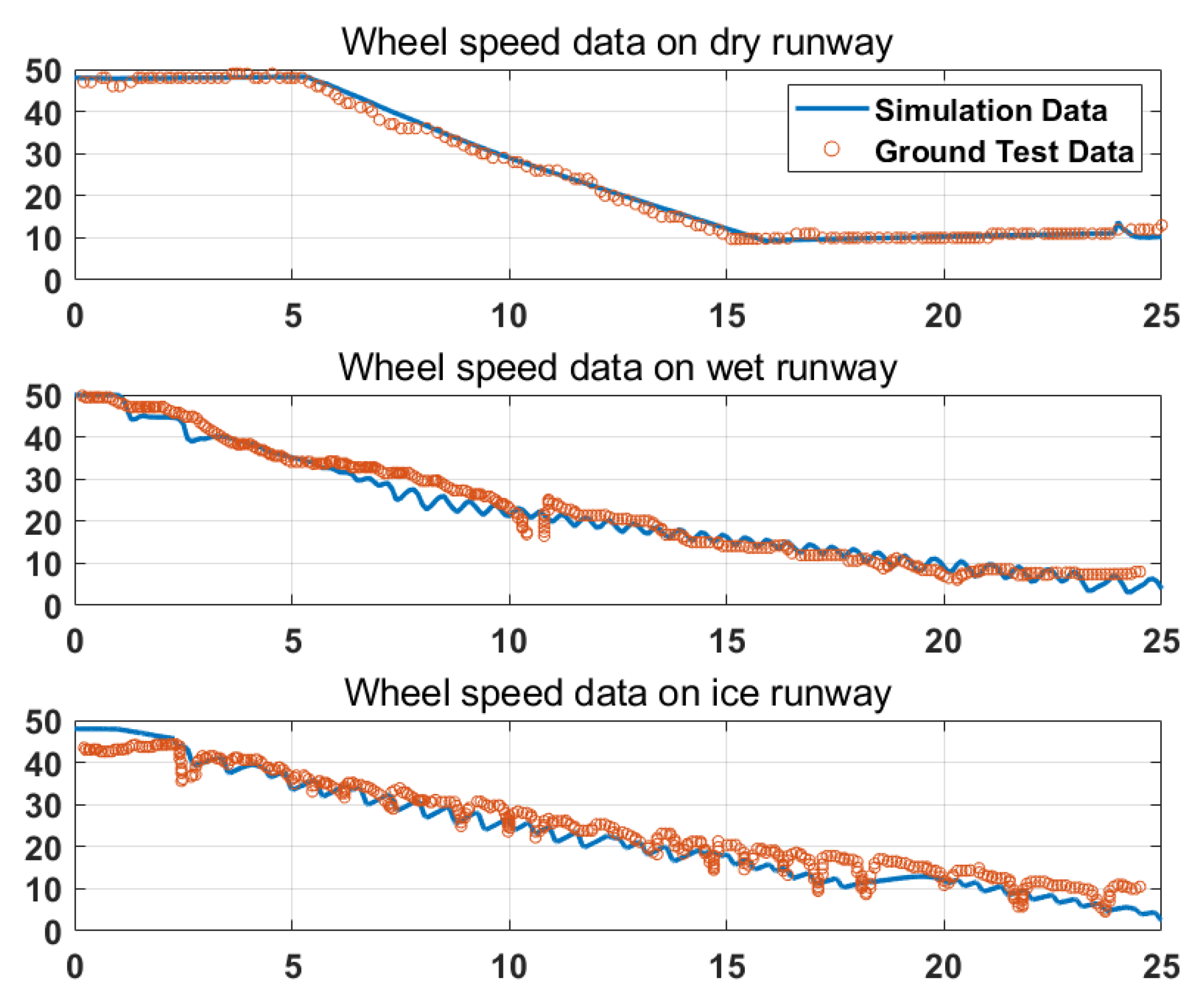
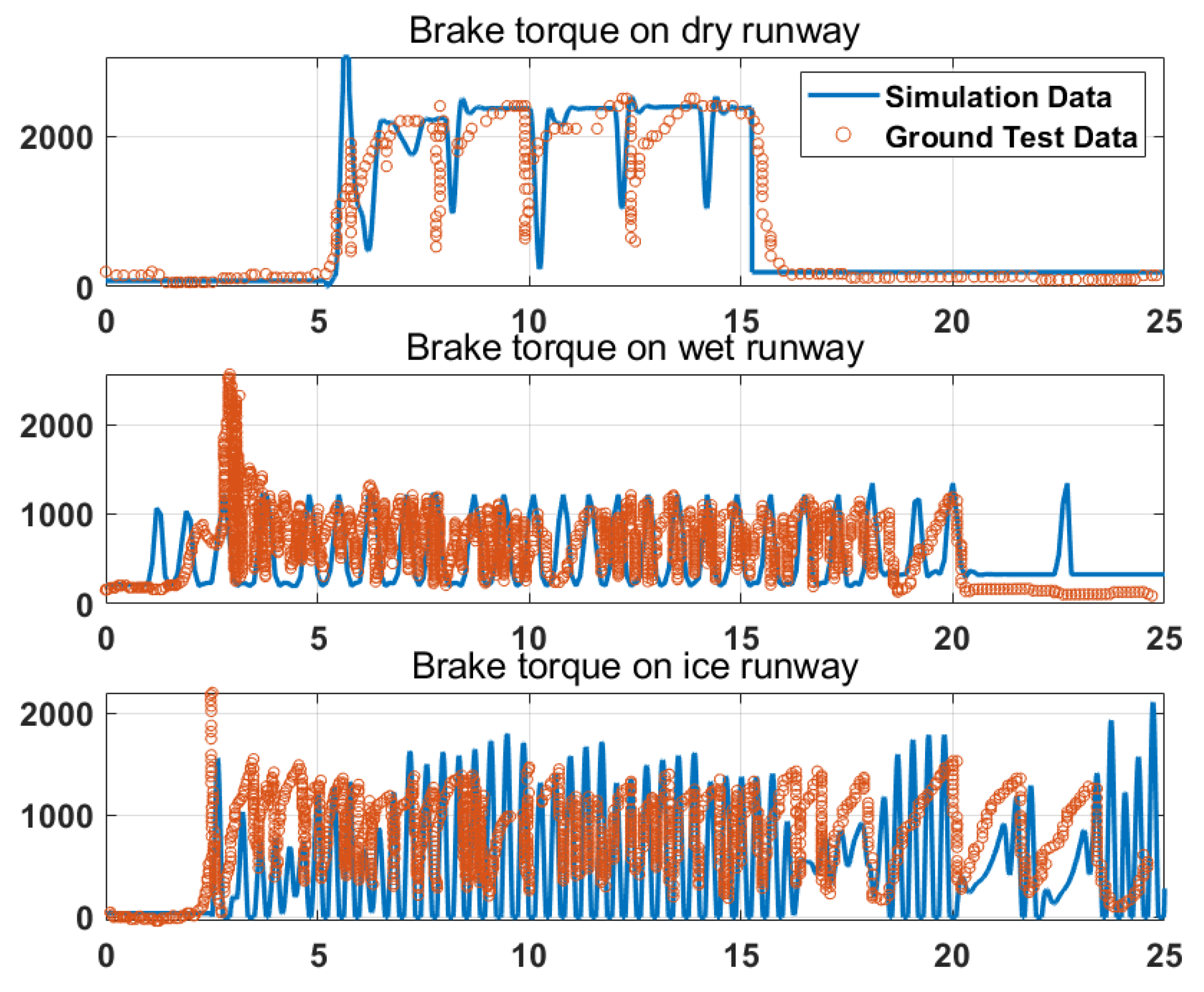
In order to verify the accuracy of the established model, the simulation results were compared with the ground test results provided by FAA and NASA. As described in [25], the FAA and NASA working together conducted extensive runway friction tests with two instrumented aircraft for a wide variety of runway surface types and conditions. The controller used in the experiment and simulation was a traditional PBM controller, which is the most commonly used braking controller in aircraft braking systems. Thus, in this paper, a PBM controller was also designed. The following results show the simulation results compared with the ground test results provided by FAA and NASA on three different runways. Some of the ground test results are given in Table 3. Figure 12 shows the test track and friction device of the NASA Langley Experiment Center, and the data in Table 3 are the experimental data on the test bench.
Figure 13, Figure 14 and Figure 15 are the results of comparisons between the simulation data and the ground test data on three commonly used runways. The controllers used in the simulation and the ground test were both PBM controllers. As indicated in the following figures, the simulation results were basically consistent with the experimental results, which indicate that the simulation model built in this paper was suitable for the test of the proposed controller. It is worth mentioning that, though no ice runway results were provided, we can use the experimental results of the flooded runway, because the maximum bonding coefficient and friction characteristics of the road surface were similar to those of the ice runway under the condition of water accumulation.
5.2. Simulation Results of the Proposed Controller
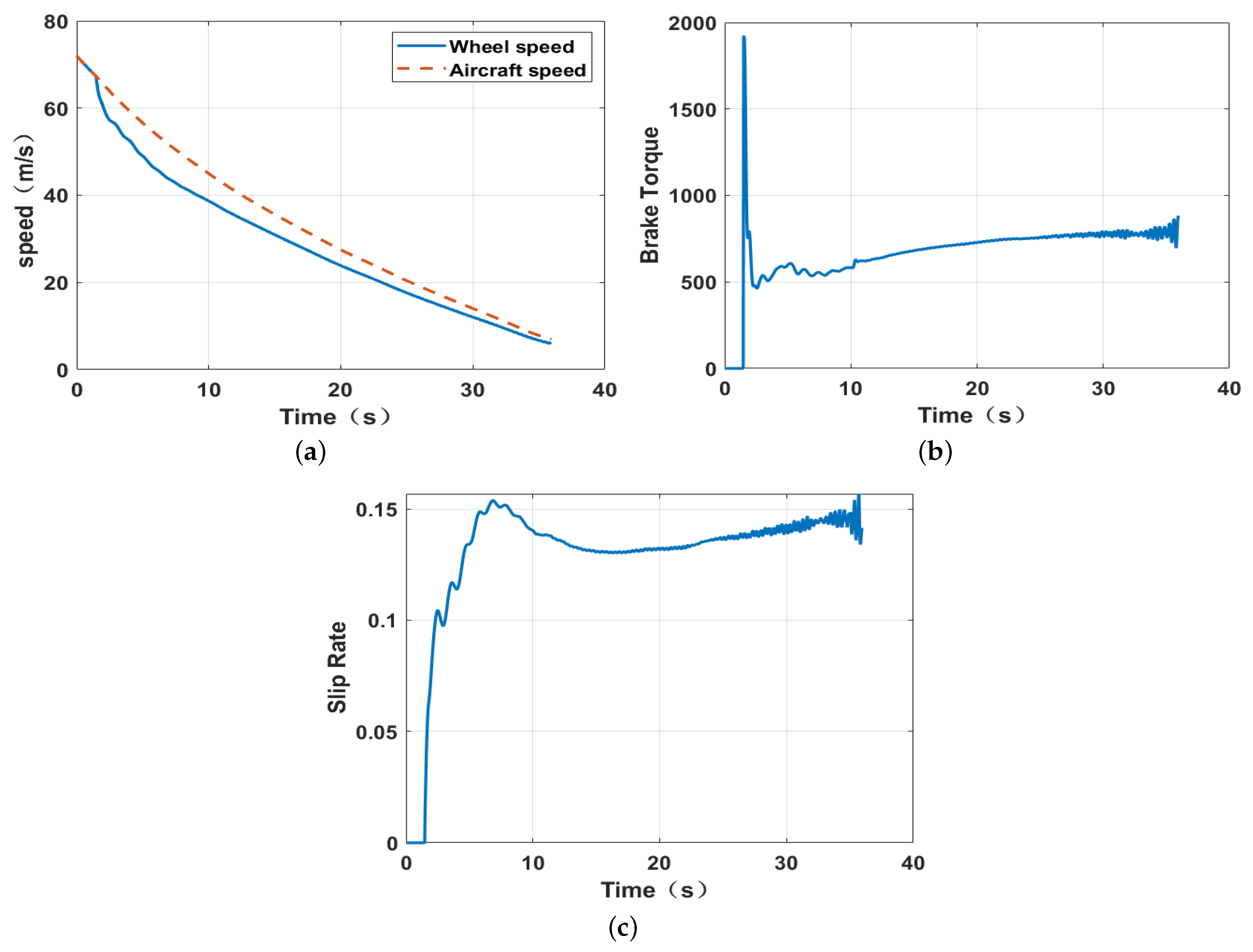
In order to verify the performance of the designed controller, a series of simulation tests was carried out in this study on the basis of the above-mentioned verified model. The initial parameters of the PSO were as follows: population size PS = 20; acceleration factor Ac1 = 1; Ac2 = 3.2; Ac3 = 0.5; maximum iteration number Ni = 30. Without a loss of generality, the test was performed under the harshest runway conditions, i.e., an ice runway. The simulation results of the proposed controller are as follows.
Figure 16 shows the simulation results under the conditions of an ice runway. For the aircraft anti-skid braking control system, the main control goal was to make full use of the friction between the tire and the ground, improve the braking efficiency, and prevent the tire from slipping and locking. Therefore, for the aircraft anti-skid system, the variables we were most concerned about were the speed of the aircraft body, the speed of the wheels, the slip rate, and the braking torque. From the above simulation results, it can be seen that, despite the harshest braking environment, the controller still showed good performance. It can be seen in Figure 16a that, during the entire braking process, there was no deep skid as shown in Figure 4, nor was there any tire lockup. Because the simulation conditions represent the most severe conditions in the industry (i.e., ice runways), we believe that, for the vast majority of logarithmic runway conditions, the controller proposed in this paper can avoid the problem of deep skid or tire locking during the braking process of the aircraft. Furthermore, as can be seen in Figure 16b, the controller can quickly adjust the output braking pressure according to the state of the runway, which means that the particle swarm optimization algorithm we designed can quickly adjust the PID parameters, and its performance can meet the real-time requirements of the anti-skid braking system. Figure 16c depicts that the slip rate of the system can quickly reach 0.12–0.15, which is the optimal slip rate interval, according to [37].
5.3. Algorithm Robustness Proof and Simulation Verification
The proof of the robustness of the controller (Equation (36)) is as follows:
Theorem 1.
Proof.
The Lyapunov function used in this paper is as follows:
Taking the derivative of Equation (40) yields
Assuming , integrating the above equation from to , yields
Because , Equation (42) implies the following inequality:
□
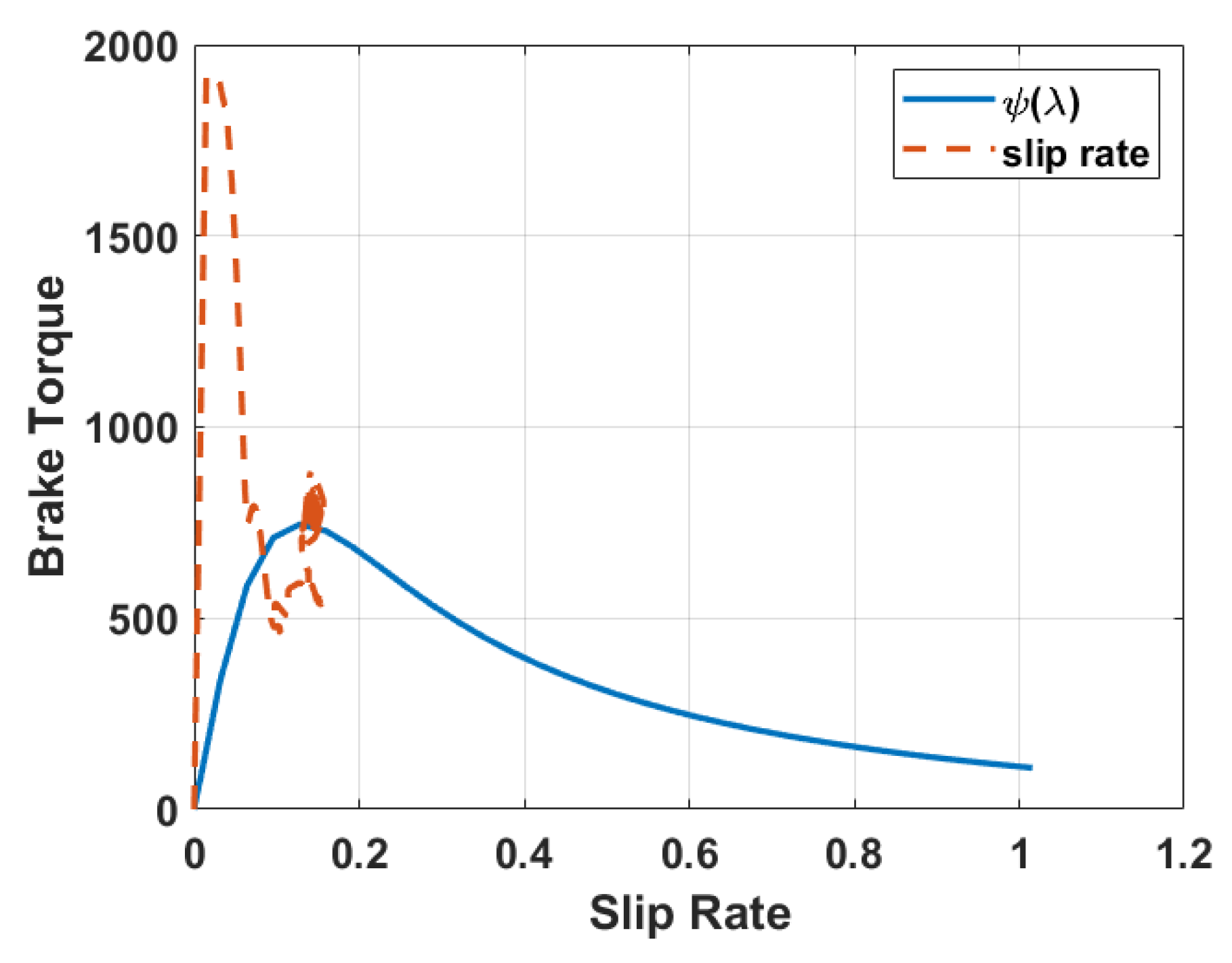
Thus, the proof is complete. In addition, to further prove the trace performance, the closed-loop trajectory of the system under control is drawn as in Figure 17. It can be seen in Figure 17 that the brake torque converged to the extreme point of (the expression of can be found in [38]), which indicates that, under the control action of the proposed controller, the braking system converged to an optimal operating point, despite the existence of model uncertainty and disturbance.
6. Conclusions
The aircraft anti-skid braking system is a very important subsystem, and its performance determines the safety of the aircraft landing process to a large extent. In this paper, a robust self-learning PID algorithm was proposed in order to make full use of the friction between the tire and the road surface, improve the braking efficiency, and prevent the tire from deep skidding or locking. The robustness of the controller was proved by the Lyapunov method. At the same time, in order to verify the overall performance of the controller in anti-skid control, a simulation model of the aircraft braking process was established based on MATLAB/Simulink. The model was validated by comparisons with NASA ground test data.
The final simulation results in Figure 17 show that the designed controller could quickly adjust the value of the system slip rate to near the optimal value, and there was no deep slippage or tire locking during the entire anti-skid process, showing favorable control performance.
This paper mainly focused on the dynamic characteristics of fuselage speed, slip rate, and braking torque in the process of anti-skid braking, but there are many characteristics worthy of study in anti-skid control, such as the characteristics of servo valves and hydraulic pipelines. Runway state identification would also be an interesting research direction.
Author Contributions
Conceptualization, W.L. and F.X.; methodology, F.X. and M.C.; software, F.X. and X.L.; validation, F.X., X.L. and M.C.; formal analysis, F.X.; investigation, W.L. and F.X.; resources, F.X.; data curation, F.X.; writing—original draft preparation, F.X.; writing—review and editing, F.X.; visualization, F.X.; supervision, W.L., F.X. and M.C.; project administration, W.L., F.X. and X.L. All authors have read and agreed to the published version of the manuscript.
Funding
This research was supported by Chang Jiang Scholars Program of Ministry of Education of China: T2011119.
Institutional Review Board Statement
Not applicable.
Informed Consent Statement
Not applicable.
Data Availability Statement
Not applicable.
Conflicts of Interest
The authors declare that there are no conflict of interest.
References
- Boeing. Statistical Summary of Commercial Jet Airplane Accidents. 2021. Available online: https://www.boeing.com/company/about-bca/aviation-safety.page/ (accessed on 1 April 2022).
- Hoseinnezhad, R.; Bab-Hadiashar, A. Efficient Antilock Braking by Direct Maximization of Tire–Road Frictions. IEEE Trans. Ind. Electron. 2011, 58, 3593–3600. [Google Scholar] [CrossRef]
- Park, G.; Choi, S.B. Clamping force control based on dynamic model estimation for electromechanical brakes. Proc. Inst. Mech. Eng. Part D J. Automob. Eng. 2018, 232, 2000–2013. [Google Scholar] [CrossRef]
- Kiencke, U.; Nielsen, L. Automotive Control Systems; Springer: Berlin/Heidelberg, Germany, 2005. [Google Scholar]
- Zheng, T.X.; Ma, F. Automotive ABS control strategy based on logic threshold. J. Traffic Transp. Eng.-Engl. Ed. 2010, 10, 69–74. [Google Scholar]
- Layne, J.R.; Passino, K.M.; Yurkovich, S. Fuzzy learning control for antiskid braking systems. IEEE Trans. Control Syst. Technol. 1993, 1, 122–129. [Google Scholar] [CrossRef]
- Liu, W.S.; Wang, X.; Yun-Zhu, M.A. A Fuzzy Neural Network Control of Anti-Skid Braking System Based on Unscented Kalman Filter (UKF). APMT 2017, 53, 25–31. [Google Scholar]
- Peric, S.; Antic, D.; Mitic, D.; Nikolic, S.; Milojkovic, M. Generalized Quasi-Orthogonal Polynomials Applied in Sliding Mode-based Minimum Variance Control of ABS. Acta Polytech. Hung. 2020, 17, 165–182. [Google Scholar] [CrossRef]
- Antic, D.; Mitic, D.; Jovanovic, Z.; Peric, S.; Milojkovic, M.; Nikolic, S. Sliding Mode Based Anti-Lock Braking System Control; Springer: Cham, Switzerland, 2016. [Google Scholar]
- Vodovozov, V.; Petlenkov, E.; Aksjonov, A.; Raud, Z. Neural Network Control of Green Energy Vehicles with Blended Braking Systems. Renew. Energy 2021, 19, 344–349. [Google Scholar] [CrossRef]
- He, H.; Wang, C.; Jia, H.; Cui, X. An intelligent braking system composed single-pedal and multi-objective optimization neural network braking control strategies for electric vehicle. Appl. Energy 2020, 259, 114172. [Google Scholar] [CrossRef]
- Lin, W.C.; Lin, C.; Hsu, P.M.; Wu, M.T. Realization of Anti-Lock Braking Strategy for Electric Scooters. IEEE Trans. Ind. Electron. 2014, 61, 2826–2833. [Google Scholar] [CrossRef]
- Incremona, G.P.; Regolin, E.; Mosca, A.; Ferrara, A. Sliding mode control algorithms for wheel slip control of road vehicles. In Proceedings of the 2017 American Control Conference (ACC), Seattle, WA, USA, 24–26 May 2017; pp. 4297–4302. [Google Scholar]
- Mishra, S.; Kumar, P.; Rahman, M.S. Optimal design for slip deceleration control in anti-lock braking system. AIP Conf. Proc. 2018, 1953, 130006. [Google Scholar]
- Mirzaei, M.; Mirzaeinejad, H. Optimal design of a non-linear controller for anti-lock braking system. Transp. Res. Part C Emerg. Technol. 2012, 24, 19–35. [Google Scholar] [CrossRef]
- Chereji, E.; Radac, M.B.; Szedlak-Stînean, A.I. Sliding Mode Control Algorithms for Anti-Lock Braking Systems with Performance Comparisons. Algorithms 2021, 14, 2. [Google Scholar] [CrossRef]
- Bhandari, R.; Patil, S.; Singh, R.K. Surface prediction and control algorithms for anti-lock brake system. Transp. Res. Part C Emerg. Technol. 2012, 21, 181–195. [Google Scholar] [CrossRef]
- Atia, M.R.A.; Haggag, S.; Kamal, A.M.M. Enhanced Electromechanical Brake-by-Wire System Using Sliding Mode Controller. J. Dyn. Syst. Meas. Control-Trans. ASM 2016, 138, 041003. [Google Scholar] [CrossRef]
- Tang, Y.; Wang, Y.; Han, M.S.; Lian, Q. Adaptive Fuzzy Fractional-Order Sliding Mode Controller Design for Antilock Braking Systems. J. Dyn. Syst. Meas. Control-Trans. ASM 2016, 138, 041008. [Google Scholar] [CrossRef]
- Abzi, I.; Kabbaj, M.N.; Benbrahim, M. Robust Adaptive fractional-order sliding mode controller for vehicle longitudinal dynamic. In Proceedings of the 2020 17th International Multi-Conference on Systems, Signals & Devices (SSD), Monastir, Tunisia, 20–23 July 2020; pp. 1128–1132. [Google Scholar]
- Hua, Y. Research on Adaptive Grey Sliding Mode Control Algorithm for Anti-lock Braking System of Vehicle. Com. Simu 2012, 29, 326–330. [Google Scholar]
- Nyandoro, O.T.; Pedro, J.O.; Dwolatzky, B.; Dahunsi, O.A. State Feedback Based Linear Slip Control Formulation for Vehicular Antilock Braking System. In Proceedings of the World Congress on Engineering, London, UK, 6–8 July 2011. [Google Scholar]
- Radac, M.B.; Precup, R. Data-driven model-free slip control of anti-lock braking systems using reinforcement Q-learning. Neurocomputing 2018, 275, 317–329. [Google Scholar] [CrossRef]
- Radac, M.B.; Precup, R.; Roman, R.C. Anti-lock braking systems data-driven control using Q-learning. In Proceedings of the 2017 IEEE 26th International Symposium on Industrial Electronics (ISIE), Edinburgh, UK, 19–21 June 2017; pp. 418–423. [Google Scholar]
- Yager, T.J.; Vogler, W.A.; Baldasare, P. Evaluation of Two Transport Aircraft and Several Ground Test Vehicle Friction Measurements Obtained for Various Runway Surface Types and Conditions. A Summary of Test Results from Joint FAA/NASA Runway Friction Program; NASA Technical Paper; NASA: Washington, DC, USA, 1990.
- He, Y.; Lu, C.; Shen, J.; Yuan, C. Design and analysis of output feedback constraint control for antilock braking system based on Burckhardt’s model. Assem. Autom. 2019, 39, 497–513. [Google Scholar] [CrossRef]
- He, Y.; Lu, C.; Shen, J.; Yuan, C. A second-order slip model for constraint backstepping control of antilock braking system based on Burckhardt’s model. Int. J. Model Simul. 2019, 40, 130–142. [Google Scholar] [CrossRef]
- Qiu, Y.; Liang, X.; Dai, Z. Backstepping dynamic surface control for an anti-skid braking system. Control Eng. Pract. 2015, 42, 140–152. [Google Scholar] [CrossRef]
- Jiao, Z.; Sun, D.; Shang, Y.; Liu, X.; Wu, S. A high efficiency aircraft anti-skid brake control with runway identification. Aerosp. Sci. Technol. 2019, 91, 82–95. [Google Scholar] [CrossRef]
- Jiao, Z.; Liu, X.; Shang, Y.; Huang, C. An integrated self-energized brake system for aircrafts based on a switching valve control. Aerosp. Sci. Technol. 2017, 60, 20–30. [Google Scholar] [CrossRef]
- Lin, C.M.; Lin, M.H.; Chen, C.H.; Yeung, D.S. Robust PID control system design for chaotic systems using particle swarm optimization algorithm. In Proceedings of the 2009 International Conference on Machine Learning and Cybernetics, Baoding, China, 12–15 July 2009; pp. 3294–3299. [Google Scholar]
- Du, C.; Li, F.; Yang, C.; Shi, Y.; Liao, L.; Gui, W. Multi-Phase-Based Optimal Slip Ratio Tracking Control of Aircraft Antiskid Braking System via Second-Order Sliding Mode Approach. IEEE-ASME Trans. Mechatron. 2021; early access. [Google Scholar]
- Wang, L.X. Adaptive Fuzzy Systems and Control—Design and Stability Analysis; Prentice-Hall: Hoboken, NJ, USA, 1994. [Google Scholar]
- Kennedy, J.; Eberhart, R.C. Particle swarm optimization. In Proceedings of the ICNN’95—International Conference on Neural Networks, Perth, Australia, 27 November–1 December 1995; Volume 4, pp. 1942–1948. [Google Scholar]
- Wang, D.; Tan, D.; Liu, L. Particle swarm optimization algorithm: An overview. Soft Comput. 2018, 22, 387–408. [Google Scholar] [CrossRef]
- Deng, W.; Yao, R.; Zhao, H.; Yang, X.; Li, G. A novel intelligent diagnosis method using optimal LS-SVM with improved PSO algorithm. Soft Comput. 2019, 23, 2445–2462. [Google Scholar] [CrossRef]
- Pacejka, H.B. Tire and Vehicle Dynamics, 3rd ed.; Elsevier: Oxford, UK, 2012. [Google Scholar]
- Savaresi, S.M.; Tanelli, M. Active Braking Control Systems Design for Vehicles; Springer: London, UK, 2010. [Google Scholar]
Figure 1.
Percentage of fatal accidents and onboard fatalities—2010–2020.

Figure 2.
Major accidents due to brake failure. (a) A tire blows out during braking. (b) An aircraft overruns a runway during braking.
Figure 2.
Major accidents due to brake failure. (a) A tire blows out during braking. (b) An aircraft overruns a runway during braking.

Figure 3.
Schematic diagram of a slip-velocity-controlled PBM control system.

Figure 4.
Speed profile of a PBM controller on a slippery runway.

Figure 5.
Signal transmission relationship between various modules of aircraft anti-skid brakes.

Figure 6.
Schematic diagram of the force of the aircraft body.

Figure 7.
Force analysis of the main wheel during the braking process.

Figure 8.
Different kinds of runway given by Burckhardts.

Figure 9.
Block diagram of the nonlinear control system.

Figure 10.
Flow chart of the particle swarm algorithm for adjusting the learning rate.

Figure 11.
The Simulink model established in this research.

Figure 12.
NASA Langley Aircraft Brake Experiment Center and tribosystem schematic diagram. (a) NASA Langley Aircraft Brake Experiment Center; (b) Aircraft landing tribosystem.
Figure 12.
NASA Langley Aircraft Brake Experiment Center and tribosystem schematic diagram. (a) NASA Langley Aircraft Brake Experiment Center; (b) Aircraft landing tribosystem.

Figure 13.
Comparison of ground test aircraft speed data and simulation aircraft speed data.

Figure 14.
Comparison of ground test wheel speed data and simulation wheel speed data.

Figure 15.
Comparison of ground test brake torque and simulation brake torque.

Figure 16.
Braking test of the proposed controller on an ice runway. (a) Aircraft velocity and wheel velocity. (b) Brake torque of the controller. (c) Slip rate of the system.
Figure 16.
Braking test of the proposed controller on an ice runway. (a) Aircraft velocity and wheel velocity. (b) Brake torque of the controller. (c) Slip rate of the system.

Figure 17.
Closed-loop trajectory on ice runways.


Table 1.
Aircraft parameters.
| Parameter | Description |
|---|---|
| y | Vertical displacement of the center of gravity of the fuselage |
| v | Aircraft speed |
| l | Distance from center of gravity to main wheel |
| l | Distance from center of gravity to front wheel |
| h | Height of center of gravity |
| n | Number of mainwheels |
| T | Residual thrust |
| M | Mass of aircraft |
| Airport air density | |
| C | Resistance coefficient |
| C | Lift coefficient |
| S | Aircraft windward area |
Table 2.
Parameters of several types of runways.
| Runway | ||||
|---|---|---|---|---|
| Dry asphalt | 1.2801 | 23.99 | 0.52 | 0.03 |
| Dry concrete | 1.1973 | 25.168 | 0.5373 | 0.03 |
| Wet asphalt | 0.857 | 33.822 | 0.347 | 0.03 |
| Snow | 0.1946 | 94.129 | 0.646 | 0.03 |
| Ice | 0.05 | 306.39 | 0 | 0.03 |
Table 3.
Some of the brake test data provided by NASA and FAA.
| Road Surface | Vertical Load | Initial Speed | Brake Pressure | Average Slip Rate | Total Braking Energy |
|---|---|---|---|---|---|
| Dry | 60 | 54 | 15.1 | 0.11 | 835 |
| Dry | 60 | 74 | 18.1 | 0.09 | 1342 |
| Dry | 65 | 70 | 13.2 | 0.12 | 1342 |
| Damp | 120 | 55 | 11 | 0.07 | 872 |
| Damp | 120 | 76 | 8.2 | 0.06 | 1037 |
| Damp | 120 | 102 | 7.9 | 0.05 | 1104 |
| Flooded | 59 | 53 | 5.6 | 0.11 | 289 |
| Flooded | 59 | 75 | 3.7 | 0.33 | 239 |
| Flooded | 78 | 53 | 6.2 | 0.12 | 533 |
Publisher’s Note: MDPI stays neutral with regard to jurisdictional claims in published maps and institutional affiliations. |
© 2022 by the authors. Licensee MDPI, Basel, Switzerland. This article is an open access article distributed under the terms and conditions of the Creative Commons Attribution (CC BY) license (https://creativecommons.org/licenses/by/4.0/).
Share and Cite
MDPI and ACS Style
Xu, F.; Liang, X.; Chen, M.; Liu, W. Robust Self-Learning PID Control of an Aircraft Anti-Skid Braking System. Mathematics 2022, 10, 1290. https://doi.org/10.3390/math10081290
AMA Style
Xu F, Liang X, Chen M, Liu W. Robust Self-Learning PID Control of an Aircraft Anti-Skid Braking System. Mathematics. 2022; 10(8):1290. https://doi.org/10.3390/math10081290
Chicago/Turabian StyleXu, Fengrui, Xuelin Liang, Mengqiao Chen, and Wensheng Liu. 2022. "Robust Self-Learning PID Control of an Aircraft Anti-Skid Braking System" Mathematics 10, no. 8: 1290. https://doi.org/10.3390/math10081290
Note that from the first issue of 2016, this journal uses article numbers instead of page numbers. See further details here.