Physical Modeling and Structural Properties of Small-Scale Mine Ventilation Networks ^†

Abstract

This work is devoted to the modeling and structural analysis of ventilation networks in small-scale mines using a physically oriented modeling method that ensures power conservation. Small-scale mines are common in the mineral extraction industry of underdeveloped countries and their physical characteristics are taken into account in the modeling process. The geometrical topology of the ventilation network in addition with the conservation laws of the fluid distribution along the network are considered in order to obtain a simple modeling methodology. Non-linear characteristics of the interconnected fluid dynamics represent a challenge to determine significant features of the system from a control point of view. Observability and controllability properties are analyzed by considering the structural systems approach. An structural analysis provides information based on the network topology independently of the mine parameters allowing the number of sensors and actuators to be reduced while also preserving the observability and controllability of the ventilation system. Experimental results are provided by building a small-scale ventilation network benchmark to evaluate the proposed model and its properties.

1. Introduction

The industry of underground mining is an important activity for several countries, providing resources for power generation and raw materials for the metal industry, as well as the economic support of communities in underdeveloped countries. An interesting problem in the mining field is the regulation and control of mine ventilation systems. Modeling the airflow dynamics in ventilation systems has a great relevance, not only to describe the system variables but also to design control systems regulating the airflow along the network. The geometric characteristics of the ventilation network provide useful information about the airflow relationship among the network branches, which can be exploited on the modeling of the dynamical system.

Previous works on the modeling and control of ventilation networks typically consider models based on the conservation laws in the nodes and branches of the network, represented by Kirchhoff’s algebraic equations and the non-linear relations describing the airflow dynamics. The geometric topology of the ventilation network is exploited to describe the interconnection of the dynamic variables, but generic control properties have not been analyzed.

1.1. Literature Review

The Hardy–Cross method provides a steady-state representation of mine ventilation networks analyzing the graph characteristics of the ventilation circuits and by considering Kirchhoff’s laws [1]. In [2], the linearization of a nonlinear lumped parameter model of mine ventilation systems is employed to design a multi-variable controller. The nonlinear properties of ventilation systems combined with the Kirchhoff algebraic equations are considered to design a feedback linearization strategy in [3]. This method is extended, controlling fluid networks forced periodically and including adaptive methods in [4,5]. The problem of optimal $H_1$ control is studied in [6] in order to deal with external disturbances in the ventilation circuit. A similar model is introduced in [7] to compute optimal resistance of the branches in the network with genetic algorithms applied on a feedback linearization controller. Equivalent modeling procedures are used to describe natural gas distribution networks by means of a state space representation in [8]. With a different perspective, the 1D pressure transport phenomena (advection and sink) is approximated by a ordinary differential equation with time-delay in [9,10] to be used as reference model in the controller design of the large advective flows appearing in the mining ventilation problem. The relationship between hyperbolic conservation laws in fluid networks and time-delay systems is further studied in [11].

Table 1. Literature review on mine ventilation systems modeling and control.

References	Brief Description	Model Characteristics	Strengths and Limitations
N. N. Petrov (88) [13]	To provide a systematic analysis and practical recommendations to design centralized control of the ventilation system, namely, regulate airflow by means the fan control.	Dynamic. Linear SISO plant. Transfer function with perturbations.	The control law can be designed by means of well-known linear control techniques. The model does not consider the nonlinear characteristics of the system and the complexity of the interconnected flows.
Koroleva et al. (2003–2006) [3,4,5]	Nonlinear modeling and control of fluid networks based on Kirchhoff’s conservation laws in the system. Different nonlinear control laws are designed to solve the regulation problem in the network (feedback linearization, adaptive control, etc.).	Nonlinear lumped parameter model.	Simple modeling procedure. Use of well-known control strategies. Complex behaviors such as transport phenomena and temperature convection are not taken into account.
Witrant et al. (2008–2016) [9,10,11,14,15]	Hyperbolic conservation laws. Modern control strategies are designed to provide the airflow regulation of multi-variable coupled dynamic systems (Model Predictive Control, time delay compensation, etc.)	Coupled partial differential equations and time delay systems.	Complex behaviors such as transport phenomena and temperature convection are taken into account. The complexity of the models require high computational effort.
Wang et al. (2016) [16]	Cellular automation is used to regulate the airflow in the network. The intelligent system determines the best regulating branch and fan adjustments to provide safe conditions in the mine.	Static model based on the Ventilation-On-Demand (VOD) framework.	The control system is able to adjust the branches resistances and fan input to obtain optimal results. Complex behaviors such as transport phenomena and temperature convection are not taken into account. The transient response is estimated.

provides a summary of relevant works on mine ventilation networks modeling and control. Most of the cited literature assume a full instrumented mine, namely, one in which actuators and sensors are available all along the ventilation circuit. Such an assumption is restrictive in the small-scale mining industry due to the fact that owners do not have enough earnings to purchase modern control systems and instrumentation. The lack of proper automatic control of ventilation systems can cause fatal events. For instance, the Colombian small-scale mining industry reported 124 fatal accidents in 2016 [12]. One of the main aims of the the present manuscript is to provide and define a strategy to reduce the volume of required equipment to achieve safe working conditions with an attainable cost.

1.2. Our Contribution

Our work introduces a nonlinear model for mine ventilation systems obtained from the bond-graph framework. The conservation laws appearing in the network are taken into consideration. The geometric topology of the network is closely related to the modelling procedure, allowing us to study generic characteristics of the ventilation system. Structural controllability and observability properties of the obtained model are provided. The proposed model is compared in simulation with previous results found in the literature and an experimental benchmark is used to evaluate the structural properties of the model. It is worth stressing that the characteristics and parameters of small-scale ventilation systems allow us to make the assumptions and considerations presented throughout the work.

The main contributions of the manuscript can be listed as follows:

• A simple modeling methodology based on the network interconnections which provides a reliable description of the nonlinear dynamics of flow and pressures in the network branches and nodes, respectively.
• A structural analysis of the proposed model which allows us to define the observability and controllability of the network.
• The study of generic properties of the ventilation networks allows us to define the minimum number of sensors to estimate the flow variables (flow and pressure) in all the branches and the nodes of the network, by considering the proposed model.
• The study of generic properties of the ventilation networks allows us to define the minimum number of actuators to control the flow variables (flow and pressure) in all the branches and the nodes of the network, assuming that they can supply enough power to the system, by considering the proposed model.
• Experimental results are given to demonstrate the application of the proposed modeling methodology and an estimation based on the extended Kalman filter.

The manuscript is organized as follows. Section 2 provides a mathematical description of the components of a ventilation network. In Section 3 the network nonlinear model is provided as well as a simple procedure to obtain the model matrices. Section 4 is devoted to developing an analysis from the structured systems point of view. In Section 5 the theoretical results are validated by means of experimentation in a reduced-scale ventilation test bench.

2. Physical Components

2.1. The Ventilation Network of the Mine

Ventilation systems of underground mines are designed to provide an adequate quality and quantity of airflow as well as to ensure a safe environment for workers by diluting contaminants through the mine ducts [17].

Fresh air is supplied to the mine through the down-cast ducts connected to the surface, providing clean air to the underground ventilation system and removing pollutants added to the air. The air flows out of the mine to the surface through the up-cast ducts.

Fans are installed to produce and control the airflow in the ventilation circuit. These are usually, but not necessarily, located on surface, either exhausting air through the system or connected to downcast shafts forcing air into and through the system.

The required airflow produced by the fans has an energy cost which is directly proportional to the friction opposing the passage of air. The friction depends on the size and number of mine branches and the characteristics of the interconnected nodes [18].

The airflow direction depends on the fan location and the needs associated with the transportation of the mined material such as the quantity of workers in the mining area, the amount of CO${}_2$ emissions from the mine equipment, etc. When the air flows upward through inclined ducts of the mine, the ventilation system is called ascentional, and it takes advantage of the natural ventilating effects of adding heat to the air. When the air flows in the opposite direction with respect to the natural ventilation, it is called descentional ventilation, which can be used in more compact mining systems such as long-wall faces. The descentional ventilation system can cause problems from the control point of view due to the buoyancy effects of the gases [19].

2.2. Network Branches

The ducts of the ventilation systems can be analyzed individually as a branch. The dynamics in the branch are mainly defined by the inertance of the fluid and the friction coefficient of the pipe. The following assumption is considered in this work.

Assumption 1.

The air is incompressible and the temperature in all the network is constant.

Assumption 1 is feasible due to the fact that the ducts in small-scale mines do not reach large depths, therefore low pressure and constant temperature can be considered along the network. The dynamics of the branch are characterized by the following equation:

$$L_f\frac{dQ\left(t\right)}{dt}=H\left(t\right)-RQ\left(t\right)\left|Q\left(t\right)\right|,$$

(1)

where Q is the volumetric airflow in the ventilation duct, the absolute value $|·|$ is introduced to take into consideration the airflow direction, the aerodynamic resistance is represented by $R=\rho f\Pi l/8S^3$, $\rho$ is the fluid density, f is the friction factor, $\Pi$ is the pipe perimeter, l is the pipe length and S is the cross-section area. The inertance term is $L_f=\rho l/S$ and the total pressure drop along the pipe is $H\left(t\right)=P_{in}\left(t\right)-P_{out}\left(t\right)$.

2.3. Network Nodes

When pipes are interconnected to distribute the airflow to different points of the network, a node in the network is defined as a point where at least three elements are connected, (branches and/or sources). Considering the connections in a ventilation network, the conservation of mass at the nodes can be expressed in terms of the airflow quantities, namely, the sum of airflows ingoing into the node is equal to the sum of outgoing airflows. An additional coupling condition for the intersections is that the pressure inside each node is uniform (and thus the same at each extremity of the connected pipes). Whenever the airflow is required to change direction, additional vortices will be initiated. The propagation of those large-scale eddies consumes mechanical energy and the resistance of the airway may increase [19]. For a node in the network, the following dynamics are considered:

$$C\frac{dP\left(t\right)}{dt}=\sum _{i=1}^{N_{in}}{Q}_{in}\left(t\right)-\sum _{j=1}^{N_{out}}{Q}_{out}\left(t\right)-\sqrt{\frac{P\left(t\right)}{R_{shock}}},$$

(2)

where $\sum Q_{in}\left(t\right)$ is the sum of airflows going into the node and $\sum Q_{out}\left(t\right)$ is the sum of airflows going out from the node. $N_{in}$ and $N_{out}$ are the number of branches connected to the node. The capacitance term C is introduced to represent the area where the distribution of airflow occurs. $R_{shock}$ is the resistive term producing the shock losses, such that $R_{shock}=X\rho /2S^2$, where X is a shock loss factor (dimensionless), related to the node geometry and material. For practical situations, there are available guidelines to the selection of X factors such as the offered by the handbooks of American Society of Heating, Refrigerating and Air Conditioning Engineers (ASHRAE) [19].

2.4. Sources

The fans used in the network to produce the air movement are modelled as follows. When the fan is considered as a pressure source, the dynamics in the fan branch is defined by:

$$H_f=d-R_f{Q}_f$$

(3)

where the pressure rise generated by the fan is denoted by d and the pressure head delivered to the network is given by $H_f$. The losses in the fan are defined by the resistance coefficient equivalent in the fan branch $R_f$ and the airflow quantity through the fan $Q_f$.

On the other hand, when a fan is acting directly in two or more branches, an airflow source connected to a node can be considered. The input associated with fan is then defined as

$$Q_f=\frac{1}{R_f}\left(d-H_f\right)$$

(4)

3. Proposed Model

3.1. Mathematical Model

This section provides a procedure based on the interconnection of the elements defined in the previous section. A bond-graph approach is considered, to obtain a structure that satisfies energy conservation constraints. The following assumption is done in order to have a well-defined model [19].

Assumption 2.

Only those airways that contribute to the flow of air through the system should appear in the network scheme. Hence, sealed-off areas of insignificant leakage, stagnant regions, dead-ends and headings that are ventilated locally by ducts and auxiliary fans should not be represented in the network. Moreover, all openings to the surface, including the tops of the shafts, are connected to a common pressure sink, namely, the surface atmospheric pressure.

Definition 1. 

The dynamic model of a ventilation network with m branches and n nodes can be written as follows:

$$\begin{gathered} \dot{x}\left(t\right)=\hspace{1em}\hspace{1em}\hspace{1em}\left[\begin{array}{cc}-\mathcal{K}{\mathcal{R}}_{\mathcal{B}}-{\mathcal{S}}_p& \mathcal{C}\\ \mathcal{K}& -\mathcal{C}{\mathcal{R}}_{\mathcal{N}}-{\mathcal{S}}_q\end{array}\right]x\left(t\right)+ \\ \left[\begin{array}{cc}{B}_p& 0\\ 0& B_q\end{array}\right]\left[\begin{array}{c}{P}_{in}\left(t\right)\\ Q_{in}\left(t\right)\end{array}\right] \end{gathered}$$

(5)

where $x\left(t\right)={\left[x_B\left(t\right)x_N\left(t\right)\right]}^T$, with the set of branch states $x_B\left(t\right)\in {\mathbb{R}}^m$ and the set of node states $x_N\left(t\right)\in {\mathbb{R}}^n$. According to the bond-graph approach [20,21,22,23], the states are defined by:

$$x_{B_i}\left(t\right)={\int }_0^t{P}_{i}d\sigma =L_{fi}{Q}_{i}fori=1,2,\cdots ,m,$$

(6)

$$x_{N_j}\left(t\right)={\int }_0^t{Q}_{j}d\sigma =C_j{P}_{j}forj=1,2,\cdots ,n.$$

(7)

The matrix ${\mathcal{K}\mathcal{R}}_{\mathcal{B}}=diag\left({\varphi }_1\left(t\right),{\varphi }_2\left(t\right),\cdots ,{\varphi }_m\left(t\right)\right)$, with the function ${\varphi }_i\left(t\right)=R_i\left|x_{B_i}\left(t\right)\right|/L_{f_i}^2$. The matrix ${\mathcal{C}\mathcal{R}}_{\mathcal{N}}=diag\left({\theta }_1\left(t\right),{\theta }_2\left(t\right),\cdots ,{\theta }_m\left(t\right)\right)$, with ${\theta }_j\left(t\right)=1/\sqrt{C_j{R}_{m+j}{x}_{N_j}\left(t\right)}$.

The interconnections within the network are expressed by the incidence matrix $E\in {\mathbb{R}}^{m\times n}$ as follows:

$$E_{ij}=\left\{\begin{array}{cc}1& \mathrm{if}\mathrm{branch}i\mathrm{is}\mathrm{connected}\mathrm{to}\mathrm{node}j\\ & \mathrm{and}\mathrm{the}\mathrm{flow}\mathrm{goes}\mathrm{away}\mathrm{from}\mathrm{node}j\\ & \\ -1& \mathrm{if}\mathrm{branch}i\mathrm{is}\mathrm{connected}\mathrm{to}\mathrm{node}j\\ & \mathrm{and}\mathrm{the}\mathrm{flow}\mathrm{goes}\mathrm{into}\mathrm{node}j\\ & \\ 0& \mathrm{otherwise}\end{array}\right.$$

(8)

The momentum conservation is expressed by the matrix $\mathcal{C}=E{C}_d$ with:

$$C_d=diag\left(1/C_1,1/C_2,\cdots ,1/C_n\right)$$

representing the parameters assigned to the node capacitance. The mass conservation in the nodes is defined by $\mathcal{K}=-E^T{K}_d$ with $K_d=diag\left(K_1,K_2,\cdots ,K_m\right)$, where $K_i=1/L_{f_i}$.

The number of fans in the network is given by $r=r_p+r_q$, where $r_p$ and $r_q$ are the number of pressure and flow sources, respectively. The input matrix $B_p\in {\mathbb{R}}^{m\times r_p}$ relates the pressure sources with the branches where they are connected and can be defined as follows:

$$B_{p_{ik}}=\left\{\begin{array}{cc}1& \mathrm{if}\mathrm{fan}k\mathrm{is}\mathrm{connected}\mathrm{to}\mathrm{branch}i\\ & \mathrm{and}\mathrm{the}\mathrm{fan}\mathrm{is}\mathrm{pushing}\mathrm{air}\mathrm{into}\mathrm{the}\mathrm{network}\\ & \\ -1& \mathrm{if}\mathrm{fan}k\mathrm{is}\mathrm{connected}\mathrm{to}\mathrm{branch}i\\ & \mathrm{and}\mathrm{the}\mathrm{fan}\mathrm{is}\mathrm{extracting}\mathrm{air}\mathrm{from}\mathrm{the}\mathrm{network}\\ & \\ 0& \mathrm{otherwise}\end{array}\right.$$

(9)

for $k=1,2,\cdots ,r_p$. On the other hand, $B_q\in {\mathbb{R}}^{n\times r_q}$ indicates the location of the nodes with airflow sources and can be expressed as:

$$B_{q_{jl}}=\left\{\begin{array}{cc}1& \mathrm{if}\mathrm{fan}l\mathrm{is}\mathrm{connected}\mathrm{to}\mathrm{node}j\\ & \mathrm{and}\mathrm{the}\mathrm{fan}\mathrm{is}\mathrm{pushing}\mathrm{air}\mathrm{into}\mathrm{the}\mathrm{network}\\ & \\ -1& \mathrm{if}\mathrm{fan}l\mathrm{is}\mathrm{connected}\mathrm{to}\mathrm{node}j\\ & \mathrm{and}\mathrm{the}\mathrm{fan}\mathrm{is}\mathrm{extracting}\mathrm{air}\mathrm{from}\mathrm{the}\mathrm{network}\\ & \\ 0& \mathrm{otherwise}\end{array}\right.$$

(10)

for $l=1,2,\cdots ,r_q$. The dynamic effects of the sources in the system are taken into account according to (3) and (4), and are represented by the diagonal matrices ${\mathcal{S}}_p$ and ${\mathcal{S}}_q$, respectively. The elements of the matrix ${\mathcal{S}}_p$ are given by:

$$S_{p_i}=\left\{\begin{array}{cc}{R}_{f_k}{K}_i& \mathrm{if}\mathrm{fan}k\mathrm{is}\mathrm{connected}\mathrm{to}\mathrm{branch}i\\ 0& \mathrm{otherwise}\end{array}\right.,$$

(11)

and the diagonal elements of ${\mathcal{S}}_q$ are:

$$S_{q_j}=\left\{\begin{array}{cc}\frac{1}{R_{f_l}{C}_j}& \mathrm{if}\mathrm{fan}l\mathrm{is}\mathrm{connected}\mathrm{to}\mathrm{node}j\\ 0& \mathrm{otherwise}\end{array}\right..$$

(12)

3.2. Modeling Procedure

This section provides a simple procedure to obtain the dynamic model (5) based on the physical approach given in Section 3.1 and a network scheme:

• Identify and enumerate the branches of the network.
• Obtain the parameters of the branches: resistance $R_i$, and inertance $L_{f_i}$.
• Identify and enumerate the nodes of the network, without considering the connection to the exterior of the mine (atmospheric conditions).
• Obtain the parameters of the nodes: resistance $R_j$, and capacitance $C_j$.
• Compute the incidence matrix, according to (8).
• Compute the input matrices according to (9) and (10).
• Include the fan dynamics by means of (11) and (12).

3.3. Example 1

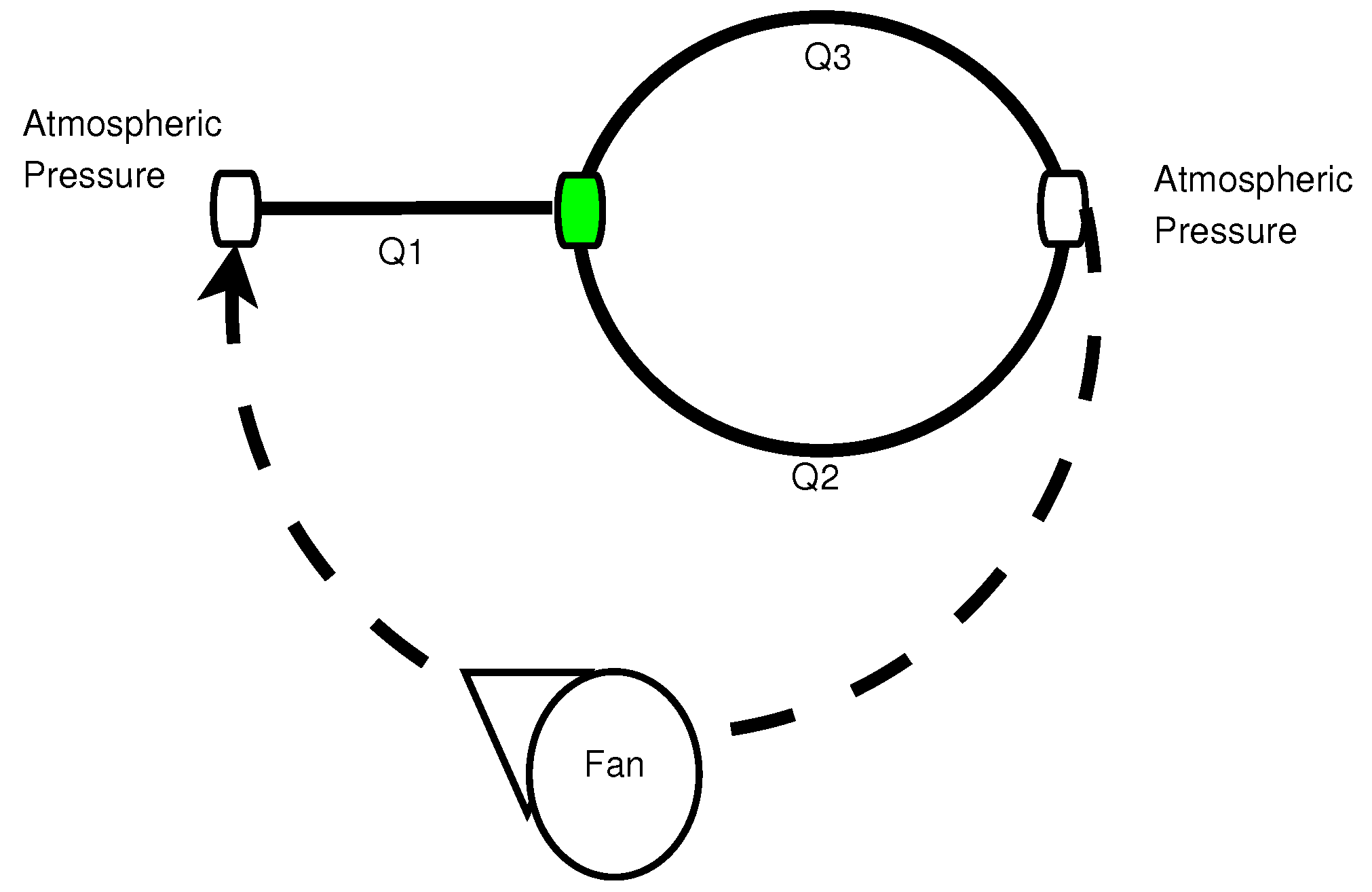
Let us consider the example presented in [3], where dimensionless magnitudes are introduced. It is worth stressing that the model proposed initially by [3] has been used in recent works to develop control strategies for mine ventilation systems [6,7,24], etc. The ventilation network represented in Figure 1 has three branches, one node and one fan. The pressure head produced by the fan is acting directly on branch 1. The flow $Q_1\left(t\right)$ is going into the node whereas the flows $Q_2\left(t\right)$ and $Q_3\left(t\right)$ are going out from the node. Then, the incidence matrix is $E={\left[-111\right]}^T$. The obtained model is given by:

$$\dot{x}=\left[\begin{array}{cccc}-{\varphi }_1-K_1{R}_f& 0& 0& -\frac{1}{C_1}\\ 0& -{\varphi }_2& 0& \frac{1}{C_1}\\ 0& 0& -{\varphi }_3& \frac{1}{C_1}\\ K_1& -K_2& -K_3& -{\theta }_4\end{array}\right]x\left(t\right)+\left[\begin{array}{c}1\\ 0\\ 0\\ 0\end{array}\right]P_{in}.$$

(13)

The dynamic model provided in [3] is used to compare the results obtained with (5). The inertance values are $K_1=1/40$, $K_2=K_3=1/10$ (kg/m${}^4$). The resistance terms are $R_1=2$, $R_2=0.35$ and $R_3=1.7$ (Ns${}^2$/m${}^8$). In [3], the shock losses in the nodes are neglected and the airflow distribution is modelled as a static relationship. To approximate such assumptions, small values of the corresponding resistance and capacitance are used, $R_{C_1}=0.001$Ns${}^2$/m${}^8$ and $C_1=0.0001$m${}^2$s${}^2$/kg. A source generating a pressure drop of $d=10$kPa is used as a fan.

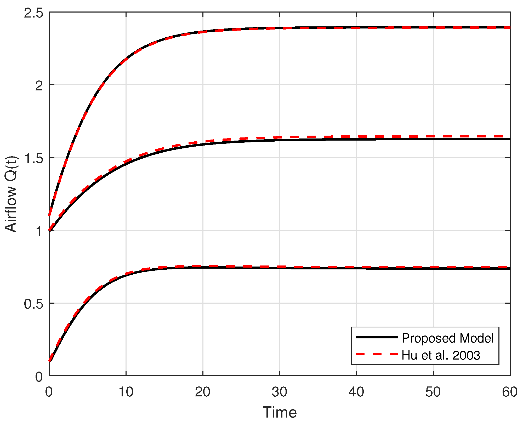
The results of the open-loop simulations are presented. In Figure 2, the mass flow rates of each branch are shown. The initial state is $Q\left(0\right)={\left[1.1,1.0,0.1,0\right]}^T$m${}^3$/s. Continuous lines are the simulation results obtained with the proposed model (5) whereas the response obtained with the model of [3] is shown by means of dashed lines.

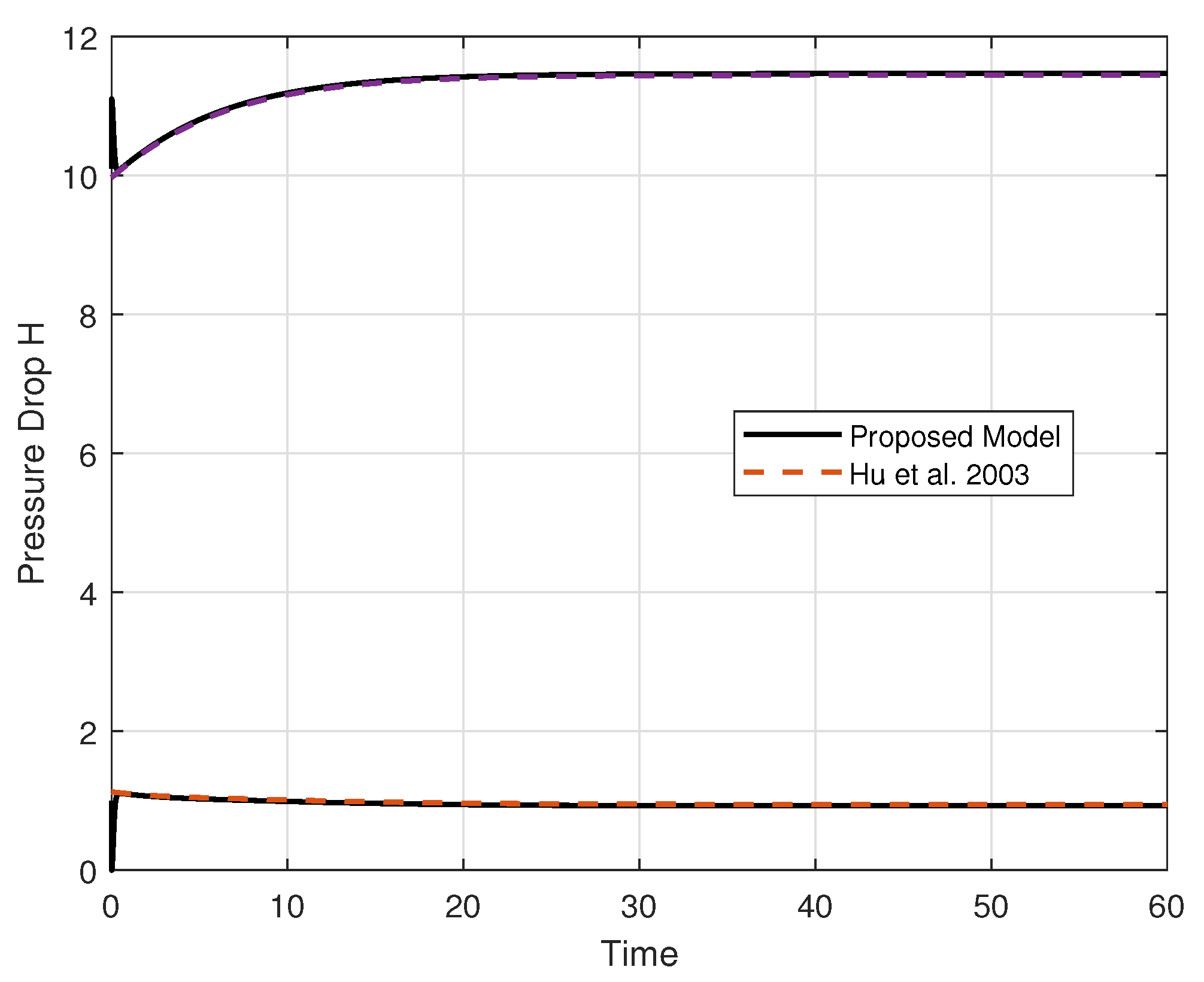
In Figure 3, the pressure rise in the branches of the network is compared. The difference between the fan input and the node pressure gives the pressure rise in branch 1, whereas the difference between node pressure and the atmospheric conditions provides the pressure rise in the branch 2, which is equal to the pressure rise in branch 3. Due to the introduction of shock losses terms in the model, a slight difference can be seen in the steady state values of the airflows and pressure drops in the network. The root mean squared error RMSE metric is used to quantify the differences between the models obtaining $RMS{E}_Q={[0.266,0.129,0.155]}^T$ for the flow signal vector and $RMS{E}_H={\left[0.2670.296\right]}^T$ for the pressure drop signal vector.

4. Structural Analysis

This section deals with the generic properties of the proposed model (5). Generic controllability and generic observability of the dynamic model of a ventilation network are analyzed from the structural systems approach.

Analyzing a system from the structural point of view allows us to capture most of the structural information available from physical laws and from the decomposition of the system into subsystems. It provides a visual representation which makes the structure clear. It allows the study of properties which depend only on the structure, almost independently of the value of the unknown parameters, these unknown parameters being in general functions of the physical values. Moreover, the computational burden is low and allows us to deal with large-scale systems, specially if they are sparse [25]. Structural analysis was developed first for linear time-invariant system. Recently, several published works were devoted to the analysis of structural properties for nonlinear networked systems [26,27,28,29,30].

4.1. Structured Systems, Structural Controllability/Observability

A structured system is a linear system of the form

$$\begin{array}{ccc}\hfill {\Sigma }_{\Lambda }:\dot{x}\left(t\right)& =& A_{\Lambda }x\left(t\right)+B_{\Lambda }u\left(t\right),\hfill \\ \hfill y\left(t\right)& =& C_{\Lambda }x\left(t\right),\hfill \end{array}$$

(14)

where the state vector $x\left(t\right)$ has dimension $\nu$, the input vector $u\left(t\right)$ has dimension $\mu$ and the output vector $y\left(t\right)$ has dimension $\tau$. Moreover, the entries of the matrices A, B and C are either fixed zeros (which determine the structure of the system) or independent parameters collected in a parameter vector $\Lambda ={({\lambda }_1,\cdots ,{\lambda }_k)}^T$. A generic property for the structured system ${\Sigma }_{\Lambda }$ is a property which is true for almost any value of $\Lambda$, see [31] for details and a rigorous definition of generic properties. It happens that a lot of important properties of ${\Sigma }_{\Lambda }$ can be characterized through a graph $G\left({\Sigma }_{\Lambda }\right)$ which can be naturally associated with ${\Sigma }_{\Lambda }$ [25]. $G\left({\Sigma }_{\Lambda }\right)$ is defined as follows:

• The vertex set is $Z=X\cup U\cup Y$ where X, U and Y are the state, input and output sets given by $X=\{x_1,x_2,\cdots ,x_{\nu }\}$, $U=\{u_1,u_2,\cdots ,u_{\mu }\}$ and $Y=\{y_1,y_2,\cdots ,y_{\tau }\}$ respectively.
• The edge set is $W=\left\{(x_i,x_j)\right|a_{{\Lambda }_{ji}}\ne 0\}\cup \left\{(u_k,x_l)\right|b_{{\Lambda }_{lk}}\ne 0\}\cup \left\{(x_p,y_q)\right|c_{{\Lambda }_{qp}}\ne 0\}$, where $a_{{\Lambda }_{ji}}$ denotes the $(j,i)$ entry of the matrix $A_{\Lambda }$, $b_{{\Lambda }_{l,k}}$ denotes the $(l,k)$ entry of $B_{\Lambda }$ and $c_{{\Lambda }_{q,p}}$ denotes the $(q,p)$ entry of of $C_{\Lambda }$.

The graph $G\left({\Sigma }_{\Lambda }\right)$ depicts the fact that some variable acts, or not, on another one.

A path in $G\left({\Sigma }_{\Lambda }\right)$ from a node $v_0$ to a node $v_q$ is a sequence of edges, $(v_0,v_1),(v_1,v_2),\dots$, $(v_{q-1},v_q)$, such that $v_t\in Z$ for $t=0,1,\dots ,q$, and $(v_{t-1},v_t)\in W$ for $t=1,2,\dots ,q$. The nodes $v_0,\cdots ,v_q$ are then said to be covered by the path. A path which does not meet the same node twice is called a simple path. If $v_0\in U$ and $v_q\in X$, the path is called an input-state path. A path for which $v_0=v_q$ is called a circuit. An input-stem is a simple input-state path. A system is said to be input-connected if any state node is the end node of an input-stem. A cycle is a circuit which does not meet the same node twice, except for the initial/end node. Two paths are disjoint when they cover disjoint sets of nodes. When some input-stems and cycles are mutually disjoint, they constitute a disjoint set of input-stems and cycles.

The following result characterises structural controllability [25,32].

Theorem 1. 

Let ${\Sigma }_{\Lambda }$ be the linear structured system defined by (14) with associated graph $G\left({\Sigma }_{\Lambda }\right)$. System ${\Sigma }_{\Lambda }$ is structurally controllable if and only if

• the graph $G\left({\Sigma }_{\Lambda }\right)$ is input-connected, and;
• the state nodes of $G\left({\Sigma }_{\Lambda }\right)$ can be covered by a disjoint set of input-stems and cycles.

The two conditions of Theorem 1 can be checked in polynomial time by standard combinatorial algorithms.

By duality, the structural observability can be checked from the observability counterpart of Theorem 1 which can be stated as follows.

Theorem 2. 

Let ${\Sigma }_{\Lambda }$ be the linear structured system defined by (14) with associated graph $G\left({\Sigma }_{\Lambda }\right)$. System ${\Sigma }_{\Lambda }$ is structurally observable if and only if

• the graph $G\left({\Sigma }_{\Lambda }\right)$ is output-connected, and;
• the state nodes of $G\left({\Sigma }_{\Lambda }\right)$ can be covered by a disjoint set of output-stems and cycles.

where output connection and output-stems are defined by changing the roles of inputs and outputs in the previous definitions.

We will see now that the model developed in the previous sections can be properly embedded in the structured system framework and that the application of the results of this theory implies important and general properties for the ventilation networks. In particular, we will see that the so-called Minimum Controllability Problem [26,33] will be solved here with a unique input.

4.2. The Ventilation Network and Its Structural Model

The nonlinear dynamic model presented in [3,4,7] is based on an algebraic transformation, consisting of the basic differential relation in the branches and Kirchhoff’s laws applied to the flows and pressure drops in the network. The obtained model has been designed to be used in feedback control strategies. Unfortunately, the variables appearing in the differential equations of the model are linear combinations of the physical parameters, rending unclear the relationships among state variables.

As seen previously, the network representation (5) directly uses the values of the physical parameters, allowing the ventilation network to be analyzed from a structural point of view. The important following statement can be obtained:

Proposition 1.

Every linear approximation of (5) has the same structure.

Let us define the linearization of (5) around an operating point:

$$x_{op}={[x_{1_0},x_{2_0},\cdots ,x_{{m+n}_0}]}^T,$$

defined by:

$$\delta \dot{x}\left(t\right)=\left[\begin{array}{cc}-K{R}_B-{\mathcal{S}}_p& \mathcal{C}\\ \mathcal{K}& C{R}_N-{\mathcal{S}}_p\end{array}\right]\delta x\left(t\right)+\left[\begin{array}{cc}{B}_p& 0\\ 0& B_q\end{array}\right]\delta u\left(t\right),$$

(15)

where $\delta x\left(t\right)$ represents the state variations around the operating point, $\delta u\left(t\right)=[\delta P_{in}\left(t\right),\delta Q_{in}\left(t\right)]$ are the variations produced by the fans around the equilibrium. The matrices are:

$$K{R}_B=diag\left(2K_1{R}_1{x}_{1_0},2K_2{R}_2{x}_{2_0},\cdots ,2K_m{R}_m{x}_{m_0}\right)$$

and

$$C{R}_N=diag\left({\varsigma }_1,{\varsigma }_2,\cdots ,{\varsigma }_n\right),$$

where

$${\varsigma }_j=\frac{R_{m+j}}{2C_j{\left(R_{m+j}{x}_{{(m+j)}_0}\right)}^{3/2}}.$$

It is appropriate to assume that at any equilibrium point all the state variables in that operation point are different from zero, i.e., there are no vacuum states in the network. In addition, all the physical parameters of the network are different from zero. Then, every linear realization of the model (5) preserves the zero/non-zero distribution in the state matrices. Moreover, the zero/non-zero distribution of the linear approximation has exactly the same structure as that of the nonlinear model (5).

The system (15) can be analyzed from the structural point of view by means of the representation (14) where the state matrices are defined as follows:

$$A_{\Lambda }=\left[\begin{array}{cc}K{R}_{\lambda }& E_{\lambda }\\ F_{\lambda }& C{R}_{\lambda }\end{array}\right],$$

(16)

with

$$K{R}_{\lambda }=\left[\begin{array}{cccc}{\lambda }_1& 0& \cdots & 0\\ 0& {\lambda }_2& \cdots & 0\\ ⋮& ⋮& \ddots & ⋮\\ 0& 0& \cdots & {\lambda }_m\end{array}\right],$$

$$C{R}_{\lambda }=\left[\begin{array}{cccc}{\lambda }_{m+1}& 0& \cdots & 0\\ 0& {\lambda }_{m+2}& \cdots & 0\\ ⋮& ⋮& \ddots & ⋮\\ 0& 0& \cdots & {\lambda }_{m+n}\end{array}\right],$$

where ${\lambda }_k$ are the nonzero free parameters. Matrices $E_{\Lambda }$ and $F_{\Lambda }$ are defined as follows:

$$E_{{\Lambda }_{ij}}=\left\{\begin{array}{cc}{\lambda }_{ij}& \mathrm{if}\mathrm{branch}i\mathrm{is}\mathrm{connected}\mathrm{to}\mathrm{node}j\\ & \\ 0& \mathrm{otherwise}\end{array}\right.$$

(17)

and

$$F_{{\Lambda }_{ji}}=\left\{\begin{array}{cc}{\lambda }_{ji}& \mathrm{if}\mathrm{branch}i\mathrm{is}\mathrm{connected}\mathrm{to}\mathrm{node}j\\ & \\ 0& \mathrm{otherwise}\end{array}\right.$$

(18)

The matrix $B_{\Lambda }$ in (14) is the input matrix and $C_{\Lambda }$ is the output matrix. Notice that matrices $E_{\Lambda }$ and $F_{\Lambda }$ have similar zero/nonzero distribution (in a transposed position). However, the parameters of $E_{\Lambda }$ are related with the capacitance in the nodes, whereas the values of $F_{\Lambda }$ are associated with the inertance in the pipes.

The matrix $B_{\Lambda }$ is defined by Equations (9) and (10). $B_{\Lambda }$ is then composed of entries which are either 0, 1 and $-1$, depending on the position and the role of the corresponding fan.

The matrix $C_{\Lambda }$ is composed depending on measurements provided by the sensors. Each row of $C_{\Lambda }$ is associated with a sensor, and this row is composed of zeros except for the state variable which is measured by the sensor.

From these observations on the matrices $A_{\Lambda }$, $B_{\Lambda }$ and $C_{\Lambda }$, it follows that the ventilation model is composed of zeros and independent entries: it can then be studied in the framework of linear structured systems.

4.3. Properties of the Ventilation Model as a Structured System

Consider a general connected ventilation network as detailed in the previous subsection, its associated structured system ${\Sigma }_{\Lambda }$ and directed graph $G\left({\Sigma }_{\Lambda }\right)$. We call $G\left(A_{\Lambda }\right)$ the sub-graph of $G\left({\Sigma }_{\Lambda }\right)$ composed of the state vertices and edges between state vertices. From the properties of the structured model, one can make the following two important observations.

• The vertex set of the graph $G\left({\Sigma }_{\Lambda }\right)$ associated with the structured model of the ventilation network (14) can be arranged in a set of branch vertices $Z_b$ given by $\{x_1,x_2,\cdots ,x_m\}$, and a set of node vertices $Z_n$ given by $\{x_{m+1},x_{m+2},\cdots ,x_{m+n}\}$. Since the model (5) is obtained by means of a power-conservation approach and considering Assumption 2, every branch vertex is connected to at least one node vertex and vice-versa. Even more, from the conservation laws in the network modeled by means of the matrix E, every branch-node pair is bi-directional, i.e., there exists a path from any branch vertex to a node vertex, and a corresponding path in the opposite direction. In other words, $G\left(A_{\Lambda }\right)$ is a strongly connected graph, i.e., there exists a directed path from any vertex to any vertex.
• On another hand, the matrix (16) has diagonal non-zero entries. Then, there exists a self-loop associated with each state vertex in the directed graph $G\left(A_{\Lambda }\right)$.

The following important and very general result can then be stated:

Theorem 3.

Let us consider the linear structured model of a connected ventilation network system given by (14), with the state matrix defined by (16). The structured system is structurally controllable through a unique input acting on an arbitrary state vertex and structurally observable trough a unique output connected to an arbitrary state vertex. As a consequence, the ventilation network can be controlled by a unique fan arbitrarily implemented in the network and can be observed by the measurement of a unique arbitrary pressure or airflow in the network.

Proof. 

From the previous observation 1, $G\left(A_{\Lambda }\right)$ is strongly connected. Define an input u and add an edge from the vertex u to an arbitrary state vertex $x_i$. From the strong connection of $G\left(A_{\Lambda }\right)$, there is a directed path from the input vertex to any state vertex of $G\left({\Sigma }_{\Lambda }\right)$ and therefore the first condition of Theorem 1 is satisfied. From observation 2, the state vertices of $G\left({\Sigma }_{\Lambda }\right)$ are covered by the set of self-loops and condition 2 of Theorem 1 is satisfied.

The result on observability is obtained in a dual way. □

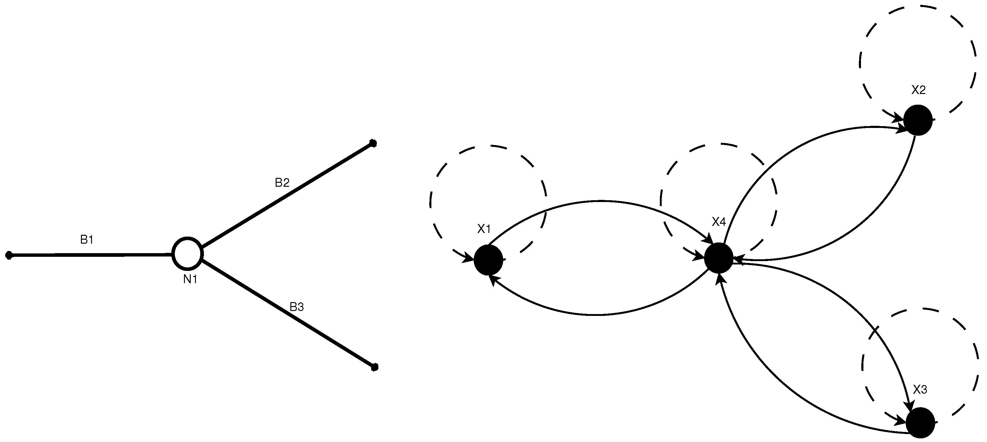
Let us consider the ventilation network shown in Figure 4 with its external ends connected to atmosphere. The corresponding structural matrix $A_{\Lambda }$ is:

$$A_{\Lambda }=\left[\begin{array}{cccc}{\lambda }_1& 0& 0& {\lambda }_5\\ 0& {\lambda }_2& 0& {\lambda }_6\\ 0& 0& {\lambda }_3& {\lambda }_7\\ {\lambda }_8& {\lambda }_9& {\lambda }_{10}& {\lambda }_4\end{array}\right]$$

independently of the location of a source (or a set of sources). Two cases can be considered. First, when the fan is connected to a branch end (as in Figure 1), the values of ${\lambda }_1=2K_1{R}_1{x}_{1_0}+K_1{R}_f$, ${\lambda }_4={\varsigma }_1$ and $B_{\Lambda }={\left[{\lambda }_{11}000\right]}^T$. On the other hand, a fan connected to the node is modelled as a flow source to be consistent with the bond-graph approach. In that case we have ${\lambda }_1=2K_1{R}_1{x}_{1_0}$, ${\lambda }_4={\varsigma }_1+1/C_j{R}_f$ and $B_{\Lambda }={\left[000{\lambda }_{11}\right]}^T$, the rest of the structural model remains the same in both cases, even if the direction of airflows changes. A similar analysis can be done with respect to the structural observability and the class of sensors used to measure the physical variables in the system.

4.4. Symmetries

Although generic properties of system (14) have been stated for a general ventilation system, there may exist cases where a particular set of free parameters ${\lambda }_k\ne 0$ induces the loss of a structural property of the system.

For instance, it can happen that an output is affected by several variables, but that these variables have the same behaviour and then the same impact on the output, which makes these variables undistinguishable. This means that there are symmetries in the differential equations, i.e., transformations of the variables that leave the equations the same [28].

In order to better understand this particularity, the following example is presented.

4.5. Example 2

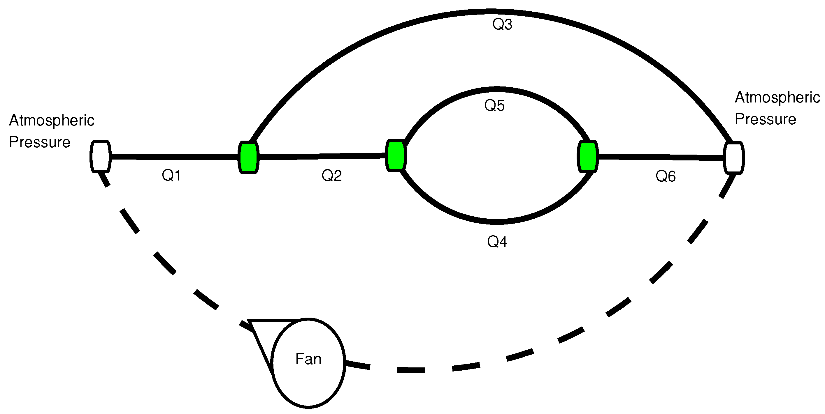
The ventilation network shown in Figure 5, with six branches and three nodes is analyzed. The parameters of the system are given in

Table 2. Parameters of the ventilation network in example 2.

Branch/Node	R [Ns${}^2$/m${}^8$]	K [kg/m${}^4$]/C [m${}^2$s${}^2$/kg]	${\mathit{Q}}_{\mathbf{ss}}$ [m${}^3$/h]/${\mathit{P}}_{\mathbf{ss}}$ [Pa]
$B_1$	0.3	0.05	10.43
$B_2$	0.22	0.1	5.62
$B_3$	0.13	0.091	4.73
$B_4$	0.09	0.083	2.33
$B_5$	0.09	0.083	2.33
$B_6$	0.17	0.067	4.57
$N_1$	0.001	0.01	6.94
$N_2$	0.0015	0.007	4.03
$N_3$	0.002	0.008	3.55

, the resistance R, the inverse of the inertance K, the capacitance C for the nodes and the steady state values for a given operation point. It can be noticed that the parameters in $B_4$ and $B_5$ are exactly the same.

An observability analysis done on the linearized system by means of Kalman’s matrix is performed. Two cases can be considered. When we use an airflow sensor located at $B_4$ and/or $B_5$, the system has complete observability, as was expected from the results provided by Theorem 3.

Even if the conditions of Theorem 2 are satisfied, placing a sensor in a different location, namely, an airflow sensor in any branch, except $B_4$ and/or $B_5$; or a pressure sensor in any node, we lose the complete observability. In fact, despite using a set of four airflow sensors located at $B_1,B_2,B_3,B_6$, and three pressure sensors located in $N_1,N_2,N_3$ in the network, the system does not have complete observability. The lost of observability is due to the symmetry produced by the parameters of $B_4$ and $B_5$; the effect of a change in the airflow coming from the state variable $Q_4$ cannot be distinguished from a change occurring at $Q_5$.

Notice that by setting a different value for the parameters in one of the ducts $B_4,B_5$, the result from the structural analysis holds: namely, one sensor located in any point of the network is enough to reconstruct the complete state of the system.

From a practical point of view, the ducts being dug in the natural earth makes it very unlikely that two ducts have exactly the same physical characteristics.

Remark 1.

According with the main result of this work stated in Theorem 3, only an actuator is enough to assure state controllability of the network. However, in a practical application the controllability would also depend on the actuator capacity. For instance, in a ventilation network it will depend on the maximum airflow and/or pressure drop provided by main fan.

5. Benchmark Application

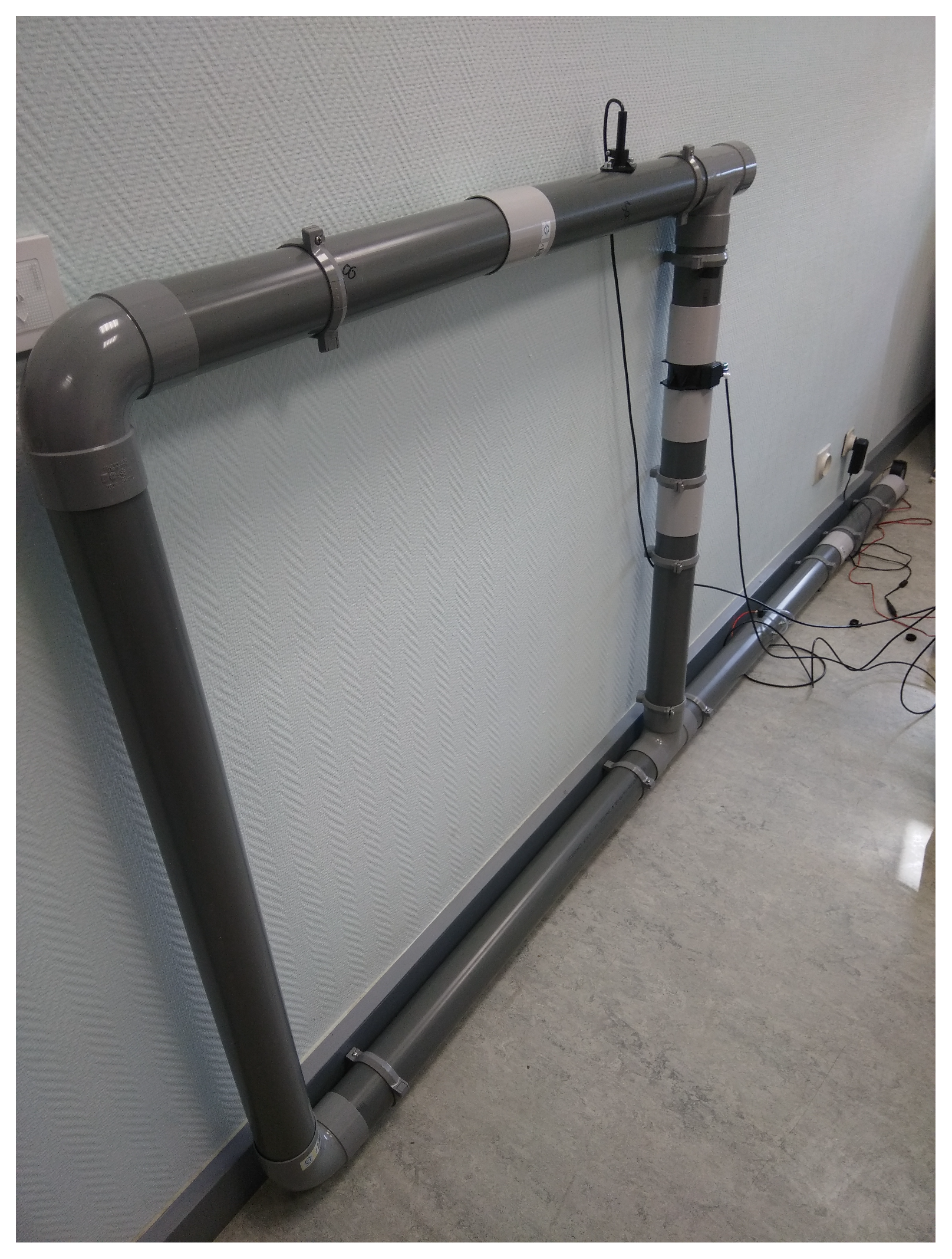
A small-scale test bench has been constructed at GIPSA-Lab to perform experimental evaluations on control strategies for ventilation networks on underground mines [18,34]. The benchmark set-up is shown in Figure 1. The network is constructed with PVC pipes and joints 80 mm in diameter. The model parameters of the experimental set-up are provided in

Table 3. Parameters of the ventilation network benchmark.

Branch	Length [m]	R [Ns${}^2$/m${}^8$]	K [kg/m${}^4$]
$B_1$	1.5	0.57	1.05
$B_2$	1	0.12	1.58
$B_3$	3	0.03	0.53

. To drive the system, a 12VDC centrifugal fan is connected to the network, providing a nominal volumetric flow of 35 ${\mathrm{m}}^3/\mathrm{h}$. The velocity of the fan can be regulated by means of a PWM signal and a H-bridge. The network has a set of sensors to measure the airflow in each branch: an orifice plate device is connected to measure the flow $Q_1\left(t\right)$ in branch 1, a mass air-flow sensor is connected in the second branch to collect the data from $Q_2\left(t\right)$ and a hot-wire sensor is used to measure $Q_3\left(t\right)$. An Arduino Mega 2560 board has been selected to be used as a data acquisition system and control unit. Figure 6 shows a picture of the ventilation network.

Estimation of internal variables in fluid networks is a challenge due to the nonlinear characteristics of the dynamical systems and the interconnection among the network variables. Recent works have been focused on this problem; for instance, in [35] the authors propose a method for state and parameter estimation of natural gas pipeline networks by considering the interconnected one-dimensional Euler equations for modeling the flow variables.

In this section, model (5) is used to estimate the state variables of the system based on the measurement of one sensor, as is stated in Theorem 3.

To evaluate the structural properties of the proposed model of the ventilation network, an Extended Kalman Filter (EKF) is used to estimate the dynamic variables of the system considering different operation points. The relation between deterministic and stochastic estimation has been analyzed, especially the possibility to obtain deterministic observers as asymptotic limits of nonlinear filters [36,37,38]. A common conclusion is that the observability condition is related to the boundedness of the error covariances in the extended Kalman filter. In particular, for the proposed nonlinear model (5) we can state the following proposition:

Proposition 2.

All the nonlinear states of the system described by (5) can be estimated by an EKF with at least a measurement on the network.

Since the results given in Proposition 1 hold, all the linear approximations described in (14) preserve observability when at least one sensor is located in the network. Then, according to the results given in [36,37,38], the EKF can be used as an observer for the nonlinear system. For more details on the EKF, see the Appendix A.

Remark 2.

The structural properties given in Section 4 are conservative in the sense that they are stated for a collection of linear approximations at the possible operation points of the nonlinear model (5). However, since the directed graph of the nonlinear system and all its linear approximations have the same structure, we obtain similar conclusions as the ones given in [26,27], where dynamic interdependence of system components through a graphical representation is considered to state observability and controllability of nonlinear networked systems.

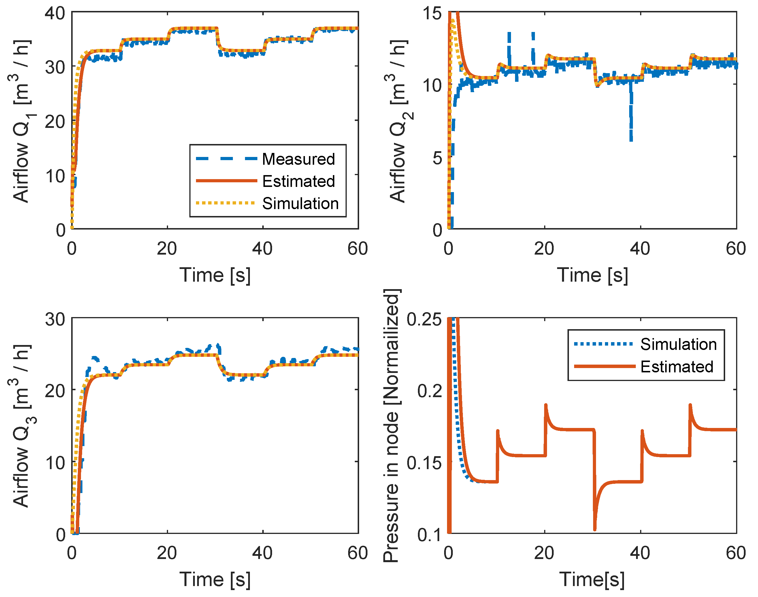
A parameter identification of each branch parameters was performed by considering a dimensionless normalized pressure in the process, i.e., a pressure in the node such that $P\left(t\right)\in [0,1]$, according to the fan operation. The network parameters are given in Table 3.

The experimental benchmark has been excited by means of a PWM signal driving the DC motor. The duty cycle of the PWM to power on the fan is changed periodically (every 10 s) at the operating conditions $PWM\in [75\%,85\%,95\%]$. Considering the network configuration, the fan is modeled as a pressure source connected to a branch. The values of the resistance in the branches are unknown as well as the nominal pressure rise provided by the fan.

Figure 7 shows the experimental results. The dashed line is used to indicate the data measured from the sensors available in the network. The solid line shows the estimation obtained by means of the extended Kalman filter which uses only the data provided by the sensor located in the first branch $Q_1\left(t\right)$, to estimate the dynamics of $Q_2\left(t\right)$, $Q_3\left(t\right)$ and the pressure in the node $P\left(t\right)$. The dotted line shows the model dynamics obtained by simulating the nonlinear model (5). There is no sensor to measure the node pressure: only the estimation and the simulated dynamics are shown. It can be seen that one sensor is enough to estimate all the state variables of the system, which is consistent with the propositions obtained from our structural analysis.

6. Conclusions and Future Work

A model of mine ventilation systems is proposed in this work. The networked nonlinear dynamics are described by means of a power conservative approach that captures the transients of the system. Simple guidelines to obtain the network model considering the branch and node interconnections and the geometric characteristics of the system are given. The proposed model allows us to analyze the generic properties of the ventilation system, obtaining interesting conclusions on the structural controllability and observability for ventilation systems. The proposed model is compared with a typical mine ventilation model found in literature, obtaining similar results. A benchmark is used to evaluate the proposed model and its structural properties. Even if the proposed results are directed to mine ventilation systems, the modeling procedure can be applied to interconnected systems distributing a different incompressible fluid, holding the studied structural properties of the network.

The results provided by the structural analysis allows us to determine the minimum number of sensors necessary estimate flow and pressure of the ducts all along the ventilation network as well as the number of actuators in the system to maintain the airflow according to the needs of flow in the working area. The results are directed to reduce the cost of control equipment of ventilation systems in small-scale mines which are common in underdeveloped countries, improving the safety conditions for the workers.

Design and validation of control and estimation strategies with a reduced number of sensors and actuators is considered for future work. The presence of dangerous gases in the mine, such as CO${}_2$ or NO${}_x$, is an interesting topic related to the transport phenomena. The estimation of hazardous gas concentrations can be further analyzed by considering the results proposed in this work.

References

- Cross, H. Analysis of Flow in Networks of Conduits or Conductors; University of Illinois, Engineering Experiment Station: Champaign, IL, USA, 1936. [Google Scholar]
- Petrov, N.; Shishkin, M.; Dmitriev, V.; Shadrin, V. Modeling mine aerology problems. J. Min. Sci. 1992, 28, 185–191. [Google Scholar] [CrossRef]
- Hu, Y.; Koroleva, O.I.; Krstic, M. Nonlinear control of mine ventilation networks. Syst. Control Lett. 2003, 49, 239–254. [Google Scholar] [CrossRef]
- Koroleva, O.; Krstic, M. Averaging analysis of periodically forced fluid networs. Automatica 2005, 41, 129–135. [Google Scholar]
- Koroleva, O.; Krstic, M.; Schmid-Schonbein, G.W. Decentralized and adaptive control of nonlinear fluid flow networks. Int. J. Control 2006, 79, 1495–1504. [Google Scholar] [CrossRef]
- Zhu, H.; Song, Z.; Hao, Y.; Feng, S. Application of Simulink Simulation for Theoretical Investigation of Nonlinear Variation of Airflow in Ventilation Network. Procedia Eng. 2012, 43, 431–436. [Google Scholar] [CrossRef] [Green Version]
- Sui, J.; Yang, L.; Hu, Y. Complex fluid network optimization and control integrative design based on nonlinear dynamic model. Chaos Solitons Fractals 2016, 89, 20–26. [Google Scholar] [CrossRef]
- Alamian, R.; Behbahani-Nejad, M.; Ghanbarzadeh, A. A state space model for transient flow simulation in natural gas pipelines. J. Nat. Gas Sci. Eng. 2012, 9, 51–59. [Google Scholar] [CrossRef]
- Witrant, E.; Marchand, N. Modeling and Feedback Control for Air Flow Regulation in Deep Pits. In Mathematical Problems in Engineering Aerospace and Sciences; Scientific Monographs and Text Books; Cambridge Scientific Publishers: Cambridge, UK, 2008. [Google Scholar]
- Witrant, E.; Niculescu, S.I. Modeling and control of large convective flows with time-delays. Math. Eng. Sci. Aerosp. 2010, 1, 191–205. [Google Scholar]
- Novella-Rodriguez, D.; Witrant, E.; Sename, O. Control-Oriented Modeling of Fluid Networks: A Time-Delay Approach; Recent Results on Nonlinear Delay Control Systems; Springer: Berlin/Heidelberg, Germany, 2016. [Google Scholar]
- Díaz, O.O.R.; Mejía, E.F.; Salamanca, J.M. Safety in underground coal mining—A look from the control systems. In Proceedings of the 2017 IEEE 3rd Colombian Conference on Automatic Control (CCAC), Cartagena, Colombia, 18–20 October 2017; pp. 1–6. [Google Scholar]
- Petrov, N.N. Automation of mine ventilation and development of main fan control systems. Sov. Min. Sci. (Engl. Transl.) 1988, 23, 79–88. [Google Scholar] [CrossRef]
- Witrant, E.; Johansson, K. Air flow modeling in deepwells: Application to mining ventilation. In Proceedings of the IEEE International Conference on Automation Science and Engineering, Washington, DC, USA, 23–26 August 2008; pp. 845–850. [Google Scholar]
- Castillo, F.; Witrant, E.; Dugard, L. Dynamic boundary stabilization of linear parameter varying hyperbolic systems: Aplicattion to a Pousille Flow. In Proceedings of the IFAC Joint Conference 11st Workshop on Time Delay Systems, Grenoble, France, 4–6 February 2013. [Google Scholar]
- Wang, K.; Jiang, S.; Wu, Z.; Shao, H.; Zhang, W.; Pei, X.; Cui, C. Intelligent safety adjustment of branch airflow volume during ventilation-on-demand changes in coal mines. Process Saf. Environ. Prot. 2017, 111, 491–506. [Google Scholar] [CrossRef]
- Wallace, K.; Prosser, B.; Stinnette, J.D. The practice of mine ventilation engineering. Int. J. Min. Sci. Technol. 2015, 25, 165–169. [Google Scholar] [CrossRef]
- Rodriguez-Diaz, O.; Novella-Rodriguez, D.; Witrant, E.; Franco-Mejia, E. Control strategies for ventilation networks in small-scale mines using an experimental benchmark. Asian J. Control 2020, 23, 72–81. [Google Scholar] [CrossRef]
- McPherson, M. Subsurface Ventilation and Environmental Engineering, 1st ed.; Springer: Dordrecht, The Netherlands, 1993. [Google Scholar]
- Borutzky, W. Bond Graph Methodology: Development and Analysis of Multidisciplinary Dynamic System Models; Springer: London, UK, 2010. [Google Scholar]
- Thoma, J.; Mocellin, G. Simulation with Entropy in Engineering Thermodynamics, Understanding Matter and Systems with Bondgraphs; Springer: Berlin/Heidelberg, Germany, 2006. [Google Scholar]
- Das, S. Mechatronic Modeling and Simulation Using Bond Graphs, 1st ed.; CRC Press, Inc.: Boca Raton, FL, USA, 2009. [Google Scholar]
- Duindam, V.; Macchelli, A.; Stramigioli, S.; Bruyninckx, H. Modeling and Control of Complex Physical Systems: The Port-Hamiltonian Approach; Springer: Berlin/Heidelberg, Germany, 2014. [Google Scholar]
- Hongqing, Z.; Zeyang, S.; Meiqun, Y.; Zheng, L.; Jian, L. Theory Study on Nonlinear Control of Ventilation Network Airflow of Mine. Procedia Eng. 2011, 26, 615–622. [Google Scholar] [CrossRef]
- Dion, J.M.; Commault, C.; van der Woude, J. Generic properties and control of linear structured systems: A survey. Automatica 2003, 39, 1125–1144. [Google Scholar] [CrossRef]
- Liu, Y.; Slotine, J.; Barabasi, A. Controllability of complex networks. Nature 2011, 473, 167–173. [Google Scholar] [CrossRef]
- Liu, Y.; Slotine, J.; Barabási, A. Observability of complex systems. Proc. Natl. Acad. Sci. USA 2013, 110, 2460–2465. [Google Scholar] [CrossRef] [Green Version]
- Anguelova, M.; Karlsson, J.; Jirstrand, M. Minimal output sets for identifiability. Math. Biosci. 2012, 239, 139–153. [Google Scholar] [CrossRef]
- Zhao, C.; Wang, W.; Liu, Y.; Slotine, J. Intrinsic dynamics induce global symmetry in network controllability. Sci. Rep. 2015, 5, 8422. [Google Scholar] [CrossRef] [Green Version]
- Stigter, J.; Joubert, D.; Molenaar, J. Observability of Complex Systems: Finding the Gap. Sci. Rep. 2017, 7, 16566. [Google Scholar] [CrossRef]
- Murota, K. Systems Analysis by Graphs and Matroids; Vol. 3, Algorithms and Combinatorics; Springer: New York, NY, USA, 1987. [Google Scholar]
- Lin, C. Structural controllability. IEEE Trans. Autom. Control 1974, 19, 201–208. [Google Scholar]
- Olshevsky, A. Minimal Controllability Problems. IEEE Trans. Control Netw. Syst. 2014, 1, 249–258. [Google Scholar] [CrossRef] [Green Version]
- Rodriguez-Diaz, O.; Novella-Rodriguez, D.; Witrant, E.; Franco-Mejia, E. Benchmark for analysis, modeling and control of ventilation systems in small-scale mine. In Proceedings of the International Conference on Control, Automation and Diagnosis (ICCAD), Grenoble, France, 2–4 July 2019; pp. 198–203. [Google Scholar]
- Sundar, K.; Zlotnik, A. State and Parameter Estimation for Natural Gas Pipeline Networks using Transient State Data. IEEE Trans. Control Syst. Technol. 2019, 27, 2110–2124. [Google Scholar] [CrossRef] [Green Version]
- Reif, K.; Unbehauen, R. The extended Kalman filter as an exponential observer for nonlinear systems. IEEE Trans. Signal Process. 1999, 47, 2324–2328. [Google Scholar] [CrossRef]
- Boutayeb, M.; Rafaralahy, H.; Darouach, M. Convergence analysis of the extended Kalman filter used as an observer for nonlinear deterministic discrete-time systems. IEEE Trans. Autom. Control 1997, 42, 581–586. [Google Scholar] [CrossRef]
- Deza, F.; Busvelle, E.; Gauthier, J.; Rakotopara, D. High gain estimation for nonlinear systems. Syst. Control Lett. 1992, 18, 295–299. [Google Scholar] [CrossRef]
- Simon, D. Optimal State Estimation. Kalman, H∞ and Nonlinear Approaches; John Wiley & Sons: Hoboken, NJ, USA, 2006. [Google Scholar]
Figure 1.
Small-scale ventilation system of a mine.
Figure 2.
Model comparison on the mass flow rate in the ventilation network [3].
Figure 3.
Model comparison on the pressure rises in the ventilation network [3].
Figure 4.
Relation between the mine scheme (left) and the directed graph (right).
Figure 5.
Scheme of a mine with six branches and three nodes.
Figure 6.
Experimental set-up of a ventilation network: The benchmark is built to emulate conditions in a typical small mine, a scale 1:500 has been used in order to configure the crosssection of the tunnels.
Figure 7.
State estimation with an Extended Kalman Filter.