MHD Mixed Convection Hybrid Nanofluids Flow over a Permeable Moving Inclined Flat Plate in the Presence of Thermophoretic and Radiative Heat Flux Effects

Abstract

Recent nanotech advancements have created a tremendous platform for the development of a superior ultrahigh performance coolant referred to as nanofluid for several industrial and engineering technologies. In this research, the impact of thermophoretic and viscous dissipation on the radiative mixed convective flow comprising hybrid nanofluid through an inclined permeable moving flat plate with a magnetic field is examined numerically. A model of non-linear differential equations is derived based on some realistic assumptions and tackled numerically using the bvp4c technique. The impact of the specific set of distinguished parameters on the velocity profiles, shear stress, temperature distribution profiles, heat transfer, concentration distribution profile, and mass transfer for the two dissimilar branch solutions are discussed in detail. In addition, it has been discovered that double solutions exist in the case of an opposing flow, while a single solution is observed in the case of an assisting flow. The temperature distribution profile escalates with the radiation parameter, while decelerating the velocity and concentration profiles.

1. Introduction

Nanotechnology is a rapidly expanding field in this modern age of advancement, where things are becoming smaller in size and getting better in the terminology of appropriate features. An area of particular importance is the preparation of products at the atomic and molecular levels for specific industrial purposes. One of the main ingredients of nanotechnology is nanofluid, which is primarily utilized to handle heat transfer challenges effectively. Thermal management of extremely sensitive systems is a major challenge in today’s engineering and science operations, such as thermal power plants, nuclear reactions, and technologically advanced procedures. A nanofluid is formed by combining some regular fluids (kerosene oil, water, alcohol, etc.) with solid nanoparticles ranging in size from 1 to 100 nm. The credit for this large-scale advancement is given to the initial research of Choi and Eastman [1], where they developed the nanofluid concept. According to Eastman et al. [2], the deferment of Cu nanoparticles increases the conduction capacity of engine oil by 40%. The primary reason for this finding is that Cu has 3000 times the thermal conductivity of engine oil. Vajravelu et al. [3] elaborated the concept of the boundary layer (BL) flow of nanofluids using Cu and Ag as nanoparticles. Makinde and Aziz [4] investigated the behavior of nanofluids flowing past a stretchable sheet while taking the convective boundary condition into account. The time-dependent flow of a nanofluid near a stagnation point was inspected by Bachok et al. [5]. The unsteady/steady flow of a nanofluid through a movable surface in a consistent exterior free stream was investigated by Roşca and Pop [6]. Reddy and Chamkha [7] examined the Dufour and Soret effects on magneto flow through a stretchable sheet induced by water-based Al₂O₃ and TiO₂ nanomaterials in porous media. The features of heat transfer for forced convection flow conveying nanomaterials through a moving plate immersed in a porous media with a heat sink/source were inspected by Ghosh and Mukhopadhyay [8]. Hussain et al. [9] presented a statistical analysis of the magnetized flow of a nanofluid through a stretchable sheet with a dissipation effect and also obtained the numerical solution. Waini et al. [10] utilized the Tiwari and Das model to scrutinize the Soret and Dufour effects on the flow of a nanofluid past a moving slim needle and presented double solutions. Hussain et al. [11] scrutinized the impact of solar radiation on the fluid flow of a non-Newtonian nanofluid immersed in a porous medium. Recently, Alazwari et al. [12] inspected the entropy generation of first-grade viscoelastic nanofluid past a porous plate. They observed that the entropy uplifts due to the volume fraction and Deborah number.

Several kinds of research have been carried out on nanofluids up to this point, but a binary hybrid nanofluid (HBN), one of the novel sorts of nanoliquid has recently piqued the interest of researchers. HBNs are made in two ways: (a) two or more dissimilar kinds of nanoparticles scattered in a regular or working base fluid, or (b) composite nanomaterials deferred in the regular fluid (conjoined). In fact, the application of nanofluid can improve heat transfer rates and lower production costs, which is why researchers are interested in this topic. The influences of convective heat transport through the tube employing a water-based Al₂O₃/Cu hybrid nanofluid were scrutinized by Suresh et al. [13] in which he discovered that hybrid nanofluids have a higher Nusselt number than regular fluids. Generally, the necessary cooling important for the electronic ingredients to avoid overheating is accomplished through the use of air-cooled heat sinks (ACHS) or liquid-CHS, with liquid-CHS being more suitable in terms of thermal efficiency. Selvakumar and Suresh [14] measured the pressure difference and rate of heat transport in an EHS using a water-based Al₂O₃/Cu hybrid nanofluid. According to their experimental outcomes, the coefficient of convective heat transport of a heat sink is augmented when hybrid nanoparticles are utilized as the working liquid. The features of heat loss through a riser pipe past a solar collector of the flat plate filled with a water-based hybrid nanofluid were inspected by Nasrin and Alim [15]. Devi and Devi [16] utilized the water-based hybrid nanofluid as well as a normal nanofluid to inspect the parametric characteristics of fluid flow past a porous stretchable sheet with a magnetic field. Ghadikolaei et al. [17] examined the transitive magnetic effect on the flow of water-based HBN past a stretching sheet with an ambient velocity and different kinds of shape factors. Huminic and Huminic [18] developed and intensely inspected the hybrid nanofluids which led to an enhancement of the thermal conductivity and ultimately an enhancement of heat transfer in the heat exchanger. The impact of the convective condition on the steady flow induced by HBN with heat transfer over a porous shrinking/stretching sheet was investigated by Waini et al. [19]. They observed that the rate of heat transfer is higher for HBN relative to a normal nanoliquid. Khan et al. [20] examined the mixed convective flow of HBN through a moving wedge with a magnetic effect and found double solutions. Roy and Pop [21] obtained an analytic solution of Stoke’s second problem induced by a water-based Cu/Al₂O₃ HBN with a heat source. The impact of a heat source/sink on magnetized flow through an exponentially stretchable sheet induced by a hybrid nanofluid was examined by Khan et al. [22]. They scattered alumina and copper nanoparticles in the blood base fluid. Recently, Khan et al. [23] discussed the axisymmetric flow and heat transport impinging on a permeable shrinkable/stretchable rotating disk conveying hybrid nanofluid and discovered a double branch outcome. Hussain [24] and Hussain et al. [25] examined the significance of a hybrid nanofluid with different aspects.

Thermophoresis refers to the phenomenon in which tiny micron-sized particles scattered in a non-isothermal gas accumulate velocity in the diminishing temperature direction. The velocity of gas molecules emerging from the warm end of the particles is higher than that of those emerging from the cold end. Collision of the molecules with the particles occurs quite vigorously, as they move more quickly. Because of the discrepancy in momentum, the particles develop a velocity in the cooler temperature direction. At first, Hales et al. [26] examined the impact of a thermophoretic assumption in the interest of engineering geometry. They inspected laminar equations through steam and aerosol transfer towards a vertical isothermal sheet. Chamkha and Pop [27] explored the role of thermophoresis particle deposition in a natural convection flow layer generated by a flat vertical plate in a porous media. Chamkha et al. [28] investigated the effect of aerosol particle thermophoresis in the laminar boundary layer through a vertical plate. Kandasamy et al. [29] analyzed the impact of irregular viscosity on magneto flow past a permeable wedge with a chemical reaction. The time-dependent flow of a micropolar fluid near a stagnation-point past a flat plate with thermophoresis and suction effects was examined by Zaib and Shafie [30]. Animasaun [31] inspected the Dufour and thermophoresis effects on magneto flow of a Casson fluid through a porous vertical plate with dissipation and temperature-dependent conductivity. Recently, Chamkha and Issa [32] scrutinized the 2D flow past a permeable semi-infinite surface subjected to a heat sink/source and thermophoresis effects.

Thermal radiation is critical in several engineering and industrial procedures such as nondestructive testing, electric power, panels of solar cells, and others. As a result, understanding the characteristic of thermal radiation is critical to achieving the preferred class of goods in industrial processes. The impact of radiation through the features of a non-Newtonian fluid with thermal diffusion and mixed convection was inspected by Mahmoud and Megahed [33]. Shehzad et al. [34] studied the thermal radiative impact on the 3D flow and heat transfer of a Jeffrey nanofluid with magnetism. Sheikholeslami and Rokni [35] investigated the roles of Coulomb force and thermal radiation in the trajectories of nanofluids in an enclosure of porous space. They discovered that the process of radiation aids in increasing the thickness of the thermal layer. Wakif et al. [36] explored the significance of the radiative effect on magneto flow of a hybrid nanofluid with effects of surface roughness. Recently, Khan et al. [37] discussed the impressions of porous media on radiative mixed convective flow induced by a hybrid nanofluid with an erratic heat sink/source from a vertical porous cylinder and presented double solutions.

As a result of the above reviews, the novelty of the current work lies in determining the numerical dual solutions of the MHD stagnation point flow induced by an HBN towards a porous moving inclined flat plate with mixed convection and thermal radiation. Moreover, the impact of viscous dissipation and thermophoretic effects are also incorporated which have not been investigated previously. The Tiwari–Das model is utilized to calculate the fine point of fluid flow. The hybrid nanofluid is created by suspending two distinct nanoparticles in the working fluids, namely silver (Ag) and titanium dioxide (TiO₂) (water). Using the similarity variables, the leadings equations and boundary conditions are later transformed into a system of ordinary differential equations, and then analysis is carried out in MATLAB using the bvp4c solver. The impacts of numerous values of the pertinent parameters on the physical quantities are demonstrated graphically, as well as in tabular form.

2. Mathematical Formulation

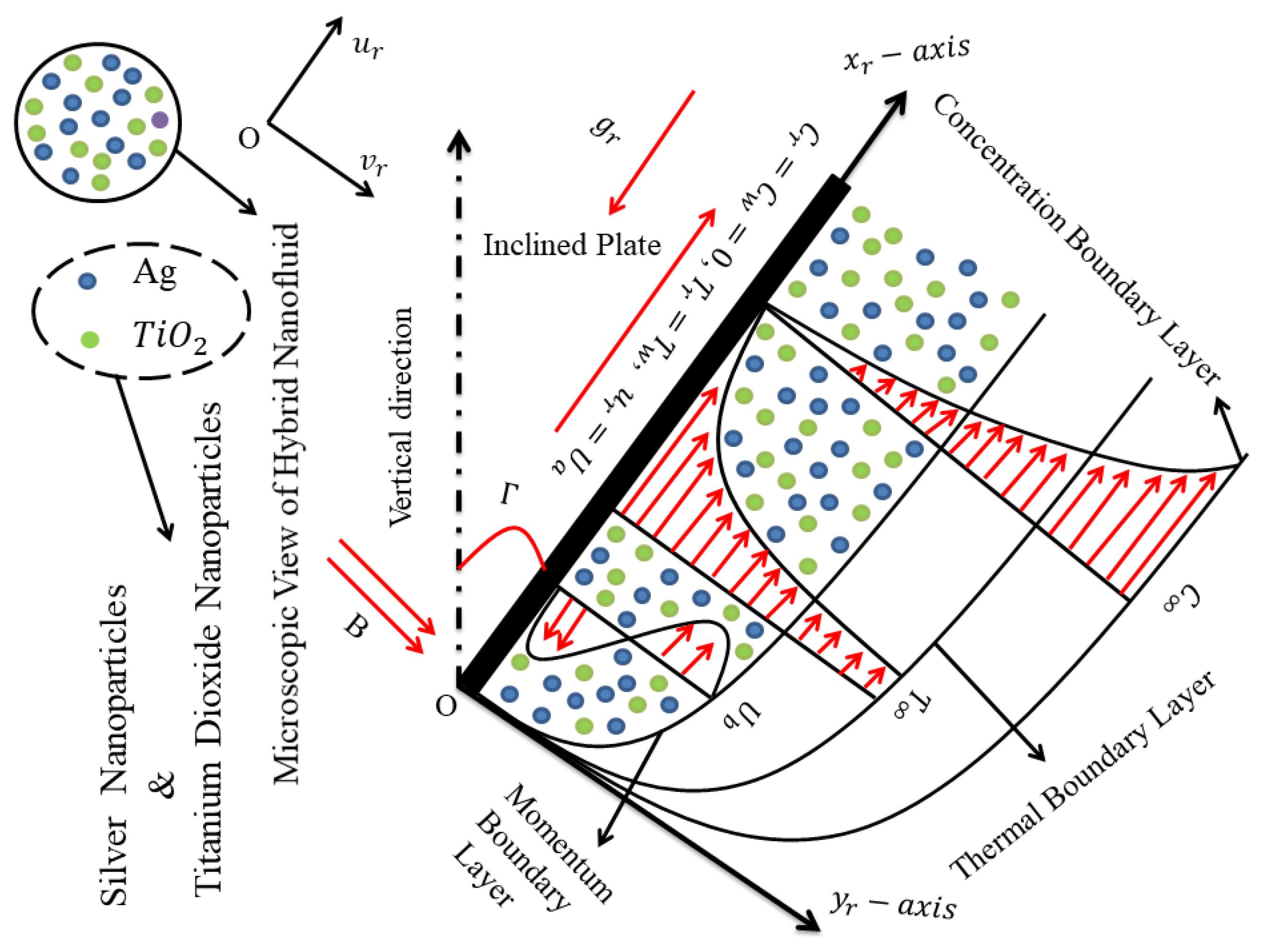
Consider a steady two-dimensional (2D) laminar flow of an incompressible electrically conducting hybrid nanofluid over a continuously moving semi-infinite inclined permeable flat plate with an acute angle $\mathsf{\Gamma }$ to the vertical, as shown in Figure 1, where, $(x_r,y_r)$ are the Cartesian coordinates with $x_r-$ and $y_r-$ being measured along the flat plate and normal to it, respectively. We assume that the velocities of the moving plate and the free stream are $U_a$ and $U_b$, respectively (in other words, the plate moves away or toward the origin with constant velocities $U_a$ and ambient velocity $U_b$), while $v_w\left(x_r\right)$ is the mass flux velocity with $v_w\left(x_r\right)>0$ for suction and $v_w\left(x_r\right)<0$ for injection, respectively, $T_w$ is the constant temperature and $C_w$ is the constant concentration of the plate, while $T_{\infty }$ and $C_{\infty }$ are the temperature and concentration of the free stream, $Q_{ra}$ is the radiative heat flux (RHF) in the $y_r$-direction. In addition, $T_w\left(x\right)<T_{\infty }$ represents the cooled plate, whereas $T_w\left(x\right)>T_{\infty }$ denotes the heated plate. For thermal enhancement, two different nanoparticles are considered, namely Ag (silver) and TiO₂ (titanium dioxide), diluted in the base working fluid (water) to form a novel class of hybrid nanofluid. A magnetic field (MF) $B\left(x_r\right)$ is applied in the $y_r$-direction. The following requisite assumptions are made:

• The particles of concentration flux are adequately undersized such that neither the temperature field nor the main velocity stream are exaggerated via the thermo-physical processes practiced by the moderately small number of particles.
• Owing to the behavior of the BL, the gradient of temperature is greater in the $y_r$-direction than the $x_r$-direction. As a result, only the component of thermophoretic velocity perpendicular to the surface is significant.
• The particle diffusivity is assumed to be constant, and the particle concentration is low enough that particle clotting in the BL is assumed to be negligible.
• The Bossiness approximation may be adopted for steady laminar flow.
• The magnetic Reynolds number (MRN) is taken to be small enough that the IMF is insignificant in comparison to the AMF.

The considered fluid is measured to be gray, representing an absorbing–emitting but non-scattering medium, and the Rosseland approximation (RAN) is exercised to describe a $Q_{ra}$ in the $x_r$-direction that is measured to be negligible relative to the $y_r$-direction. It is also assumed that $B\left(x_r\right)=B_0/\sqrt{2\left(x_r/l_r\right)}$ where $B_0$ is the constant strength of the magnetic field and $l_r$ is the characteristic length of the plate. Under the above stated conditions, the steady continuity, the momentum, the energy, and the concentration boundary layer equations of the hybrid nanofluid, in Cartesian coordinates $(x_r,y_r)$, can be written as (see Noor et al. [38]):

$$\frac{\partial u_r}{\partial x_r}+\frac{\partial v_r}{\partial y_r}=0$$

(1)

$$u_r\frac{\partial u_r}{\partial x_r}+v_r\frac{\partial u_r}{\partial y_r}=\frac{{\mu }_{hbnf}}{{\rho }_{hbnf}}\frac{{\partial }^2{u}_r}{\partial y_r^2}+\frac{{\left(\rho \beta \right)}_{hbnf}}{{\rho }_{bf}}\left(T_r-T_{\infty }\right)g_r\cos \mathsf{\Gamma }-\frac{{\sigma }_{hbnf}}{{\rho }_{bf}}{B}^2\left(x_r\right)\left(u_r-U_b\right)$$

(2)

$$\begin{array}{l}{u}_r\frac{\partial T_r}{\partial x_r}+v_r\frac{\partial T_r}{\partial y_r}=\frac{k_{hbnf}}{{\left(\rho c_p\right)}_{hbnf}}\frac{{\partial }^2{T}_r}{\partial y_r^2}-\frac{1}{{\left(\rho c_p\right)}_{hbnf}}\frac{\partial Q_{ra}}{\partial y_r}+\frac{{\mu }_{hbnf}}{{\left(\rho c_p\right)}_{hbnf}}{\left(\frac{\partial u_r}{\partial y_r}\right)}^2+\\ \frac{{\sigma }_{hbnf}}{{\left(\rho c_p\right)}_{hbnf}}{B}^2\left(x_r\right){\left(u_r-U_b\right)}^2\end{array}$$

(3)

$$u_r\frac{\partial C_r}{\partial x_r}+v_r\frac{\partial C_r}{\partial y_r}=D_B\frac{{\partial }^2{C}_r}{\partial y_r^2}-\frac{\partial \left(V_{TM}{C}_r\right)}{\partial y_r}$$

(4)

subject to the boundary conditions

$$\begin{array}{l}{u}_r=U_a, v_r=v_w\left(x_r\right), T_r=T_w, C_r=C_w=0 \mathrm{at} y_r=0,\\ u_r\to U_b, T_r\to T_{\infty }, C_r\to C_{\infty } \mathrm{as} y_r\to \infty .\end{array}$$

(5)

where $u_r$ and $v_r$ are the velocity components along $(x_r,y_r)$-axes, $T_r$ the temperature, and $C_r$ the concentration of the hybrid nanofluids, $g_r$ is the acceleration due to gravity, $D_B$ the molecular diffusivity of the species concentration, and $V_{TM}$ the thermophoretic velocity. Here, $C_w=0$ represents fully absorbing surface concentration, see Mills et al. [39] and Tsai [40].

Further, $k_{hbnf}$ is the thermal conductivity, ${\rho }_{hbnf}$ is the density, ${\sigma }_{hbnf}$ is the electrical conductivity, ${\mu }_{hbnf}$ is the absolute viscosity,${\left(\rho c_p\right)}_{hbnf}$ is the heat capacity, and ${\left(\rho \beta \right)}_{{}_{hbnf}}$ is the coefficient of thermal expansion, which are given by (see Ho et al. [41]; Sheremet et al. [42]).

$$\frac{k_{hbnf}}{k_{bf}}=\frac{\left[\frac{\left({\varphi }_a{k}_a+{\varphi }_b{k}_b\right)}{{\varphi }_a+{\varphi }_b}+\left\{\begin{array}{l}(D_A-1)k_{bf}+\left(D_A-1\right)\left({\varphi }_a{k}_a+{\varphi }_b{k}_b\right)\\ -\left(D_A-1\right)\left({\varphi }_a+{\varphi }_b\right)k_{bf}\end{array}\right\}\right]}{\left[\frac{\left({\varphi }_a{k}_a+{\varphi }_b{k}_b\right)}{{\varphi }_a+{\varphi }_b}+\left\{\begin{array}{l}\left(D_A-1\right)k_{bf}-\left({\varphi }_a{k}_a+{\varphi }_b{k}_b\right)\\ +\left({\varphi }_a+{\varphi }_b\right)k_{bf}\end{array}\right\}\right]},$$

(6)

$$\frac{{\mu }_{hbnf}}{{\mu }_{bf}}=\frac{1}{{\left(1-{\varphi }_a-{\varphi }_b\right)}^{2.5}}, \frac{{\rho }_{hbnf}}{{\rho }_{bf}}={\varphi }_a\left(\frac{{\rho }_a}{{\rho }_{bf}}\right)+{\varphi }_b\left(\frac{{\rho }_b}{{\rho }_{bf}}\right)+\left(1-{\varphi }_a-{\varphi }_b\right),$$

(7)

$$\frac{{\sigma }_{hbnf}}{{\sigma }_{bf}}=\frac{\left[\frac{\left({\varphi }_a{\sigma }_a+{\varphi }_b{\sigma }_b\right)}{{\varphi }_a+{\varphi }_b}+\left\{\begin{array}{l}(D_A-1){\sigma }_{bf}+\left(D_A-1\right)\left({\varphi }_a{\sigma }_a+{\varphi }_b{\sigma }_b\right)\\ -\left(D_A-1\right)\left({\varphi }_a+{\varphi }_b\right){\sigma }_{bf}\end{array}\right\}\right]}{\left[\frac{\left({\varphi }_a{\sigma }_a+{\varphi }_b{\sigma }_b\right)}{{\varphi }_a+{\varphi }_b}+\left\{\begin{array}{l}\left(D_A-1\right){\sigma }_{bf}-\left({\varphi }_a{\sigma }_a+{\varphi }_b{\sigma }_b\right)\\ +\left({\varphi }_a+{\varphi }_b\right){\sigma }_{bf}\end{array}\right\}\right]},$$

(8)

$$\frac{{\left(\rho c_p\right)}_{hbnf}}{{\left(\rho c_p\right)}_{bf}}={\varphi }_a\left(\frac{{\left(\rho c_p\right)}_a}{{\left(\rho c_p\right)}_{bf}}\right)+{\varphi }_b\left(\frac{{\left(\rho c_p\right)}_b}{{\left(\rho c_p\right)}_{bf}}\right)+\left(1-{\varphi }_a-{\varphi }_b\right),$$

(9)

$$\frac{{\left(\rho \beta \right)}_{hbnf}}{{\left(\rho \beta \right)}_{bf}}={\varphi }_a\left(\frac{{\left(\rho \beta \right)}_a}{{\left(\rho \beta \right)}_{bf}}\right)+{\varphi }_b\left(\frac{{\left(\rho \beta \right)}_b}{{\left(\rho \beta \right)}_{bf}}\right)+\left(1-{\varphi }_a-{\varphi }_b\right).$$

(10)

In Equations (6)–(10), the symbol $\varphi$ is called the solid nanoparticles volume fraction (where $\varphi =0$ corresponds to a regular (viscous) fluid) and $D_A$ represents the shape factor parameter, and here the value of the shape factor is considered as $D_A=3$ (spherical). Moreover, the other notations such as ${\sigma }_{bf}$, $k_{bf}$, ${\mu }_{bf}$,${\left(\rho c_p\right)}_{bf}$,${\rho }_{bf}$, and ${\left(\rho \beta \right)}_{bf}$ are the respective electrical conductivity, thermal conductivity, viscosity, specific heat capacity, density, and thermal expansion coefficient of the base working fluid while ${\varphi }_a$ signifies the Ag (silver) nanoparticles and ${\varphi }_b$ denotes the TiO₂ (titanium dioxide) nanoparticles. The physical data of the base working fluid and the two distinct hybrid nanoparticles (Ag (silver) and TiO₂ (titanium dioxide)) are written in

Table 1. The thermophysical properties of the hybrid nanoparticles.

Properties	$\mathit{\rho }\left(\mathbf{k}\mathbf{g}/{\mathbf{m}}^3\right)$	${\mathit{c}}_{\mathit{p}}\left(\mathbf{J} \mathbf{k}\mathbf{g}\mathbf{K}\right)$	$\mathit{k} \left(\mathbf{W}/\mathbf{m}\mathbf{k}\right)$	Pr
Water	997.1	4179	0.613	6.2
Cu	8933	385	400	---
Al2O3	3970	765	40	---

.

Now, employing the RAN, the $Q_{ra}$ (RHF) can simply take the following form (see Bataller [43]; Ishak [44]; Magyari and Pantokratoras [45]);

$$Q_{ra}=-\frac{4{\sigma }_A}{3k_A}\frac{\partial T_r^4}{\partial y_r}$$

(11)

where $k_A$ and ${\sigma }_A$ signify the mean absorption coefficient and the corresponding Stefan–Boltzmann constant, respectively. In addition, by applying a Taylor series to the fourth power of $T_r^4$ about the point $T_{\infty }$, and ignoring the higher power order terms, a simplified form can be obtained as $T_r^4\cong 4T_r{T}_{\infty }^3-3T_{\infty }^4$. Using this, Equation (3) can be re-written as:

$$\begin{array}{l}{u}_r\frac{\partial T_r}{\partial x_r}+v_r\frac{\partial T_r}{\partial y_r}=\frac{k_{bf}}{{\left(\rho c_p\right)}_{hbnf}}\left(\frac{k_{hbnf}}{k_{bf}}+\frac{16{\sigma }_A{T}_{\infty }^3}{3k_A{k}_{bf}}\right)\frac{{\partial }^2{T}_r}{\partial y_r^2}+\frac{{\mu }_{hbnf}}{{\left(\rho c_p\right)}_{hbnf}}{\left(\frac{\partial u_r}{\partial y_r}\right)}^2+\\ \frac{{\sigma }_{hbnf}}{{\left(\rho c_p\right)}_{hbnf}}{B}^2\left(x_r\right){\left(u_r-U_b\right)}^2.\end{array}$$

(12)

The thermophoretic velocity $V_{TM}$ which appears in Equation (4) can be written as

$$V_{TM}=-k{\upsilon }_{bf}\frac{\nabla T_r}{T_b}=-\frac{k{\upsilon }_{bf}}{T_b}\frac{\partial T_r}{\partial y_r},$$

(13)

where $T_b$ is a reference temperature and $k$ is the thermophoretic coefficient with a range of values from 0.2 to 1.2 as designated by Batchelor and Shen [46].

Therefore, Equation (1) is fulfilled for the choice of stream function $\psi \left(x_r,y_r\right)$ defined as $u_r=\partial \psi /\partial y_r$ and $v_r=-\partial \psi /\partial x_r$.

Guided by the boundary conditions (5), we introduce the following similarity variables:

$$\psi \left(x_r,y_r\right)=\sqrt{2U_b{\upsilon }_{bf}{x}_r}F\left(\xi \right), G\left(\xi \right)=\frac{T_r-T_{\infty }}{T_w-T_{\infty }}, S\left(\xi \right)=\frac{C_r}{C_{\infty }}, \xi =y_r\sqrt{\frac{U_b}{2{\upsilon }_{bf}{x}_r}}.$$

(14)

Thus, the velocity components $\left(u_r,v_r\right)$ are given by

$$u_r=U_{b}F{}^{\prime }\left(\xi \right), v_r=-\sqrt{\frac{U_b{\upsilon }_{bf}}{2x_r}}\left(F-\xi F{}^{\prime }\right)$$

(15)

So that

$$v_w\left(x_r\right)=-\sqrt{\frac{U_b{\upsilon }_{bf}}{2x_r}}{f}_w.$$

(16)

Here, the prime symbolizes the relative derivative with respect to $\xi$, $f_w$ is the constant mass flux velocity. Therefore, the cases $f_w>0$ for suction and $f_w<0$ for injection are observed, respectively.

Substituting Equation (14) into Equations (2), (4) and (12) generates the following system of ordinary (similarity) coupled equations as follows:

$$\frac{{\mu }_{hbnf}/{\mu }_{bf}}{{\rho }_{hbnf}/{\rho }_{bf}}F{}^{‴}+F{}^{″}+\frac{{\left(\rho \beta \right)}_{hbnf}/{\left(\rho \beta \right)}_{bf}}{{\rho }_{hbnf}/{\rho }_{bf}}{\mathsf{\Sigma }}_{a}G\cos \mathsf{\Gamma }-\frac{{\sigma }_{hbnf}/{\sigma }_{bf}}{{\rho }_{hbnf}/{\rho }_{bf}}{\mathsf{\Lambda }}_a\left(F{}^{\prime }-1\right)=0$$

(17)

$$\begin{array}{l}\frac{1}{\mathrm{Pr}{\left(\rho c_p\right)}_{hbnf}/{\left(\rho c_p\right)}_{bf}}\left(\frac{k_{hbnf}}{k_{bf}}+\frac{4}{3}{R}_{ad}\right)G{}^{″}+FG{}^{\prime }+\\ E{c}_a\left(\frac{{\mu }_{hbnf}/{\mu }_{bf}}{{\left(\rho c_p\right)}_{hbnf}/{\left(\rho c_p\right)}_{bf}}F{}^{″}{}^2+\frac{{\sigma }_{hbnf}/{\sigma }_{bf}}{{\left(\rho c_p\right)}_{hbnf}/{\left(\rho c_p\right)}_{bf}}{\mathsf{\Lambda }}_a{\left(F{}^{\prime }-1\right)}^2\right)=0\end{array}$$

(18)

$$\frac{1}{S{c}_a}S{}^{″}+FS{}^{\prime }+{\delta }_a\left(G{}^{″}S+G{}^{\prime }S{}^{\prime }\right)=0$$

(19)

with associated boundary conditions:

$$\begin{array}{l}F\left(0\right)=f_w, F{}^{\prime }\left(0\right)={\epsilon }_r, G\left(0\right)=1, S\left(0\right)=0 \mathrm{at} \xi =0,\\ F{}^{\prime }\to 1, G\to 0, S\to 1 \mathrm{as} \xi \to \infty .\end{array}$$

(20)

To obtain the similarity solution of Equation (3), we presume the required case is given as ${\beta }_{bf}=\frac{{\beta }_{bf}*}{x_r}$ (see Mohamed et al. [47]), where ${\beta }_{bf}*$ is constant. In addition, Pr is the Prandtl number, $S{c}_a$ is the Schmidt number, $E{c}_a$ is the Eckert number, ${\mathsf{\Lambda }}_a$ is the magnetic parameter, $R_{ad}$ is the radiation parameter, ${\delta }_a$ is the thermophoretic parameter, and ${\mathsf{\Sigma }}_a$ is the mixed convection parameter, which are defined as

$$\begin{array}{l}\mathrm{Pr}=\frac{{\mu }_{bf}{c}_p}{k_{bf}}, S{c}_a=\frac{{\upsilon }_{bf}}{D_B}, E{c}_a=\frac{U_b^2}{c_p\left(T_w-T_{\infty }\right)}, {\mathsf{\Lambda }}_a=\frac{{\sigma }_{bf}{l}_r{B}_0^2}{{\rho }_{bf}{U}_b}, R_{ad}=\frac{4{\sigma }_A{T}_{\infty }^3}{k_A{k}_{bf}},\\ {\delta }_a=\frac{k\left(T_w-T_{\infty }\right)}{T_b}, {\mathsf{\Sigma }}_a=\frac{G{r}_{x_r}}{{\mathrm{Re}}_{x_r}^2}=\frac{2g_r{\beta }_{bf}*l_r\left(T_w-T_{\infty }\right)}{U_b^2},{\epsilon }_r=\frac{U_a}{U_b}\end{array}$$

(21)

with $G{r}_{x_r}=\frac{g_r{\beta }_{bf}*\left(T_w-T_{\infty }\right){\left(2x_r\right)}^3}{{\upsilon }_{bf}^2}$ as the local Grashof number and ${\mathrm{Re}}_{x_r}=\frac{2U_b{x}_r\sqrt{x_r/l_r}}{{\upsilon }_{bf}}$ as the local Reynolds number. It should be noticed that ${\mathsf{\Sigma }}_a>0$ corresponds to assisting flow, ${\mathsf{\Sigma }}_a<0$ corresponds to opposing flow, and ${\mathsf{\Sigma }}_a=0$ corresponds to forced convection flow. In addition, ${\epsilon }_r$ is the constant moving plate parameter, with ${\epsilon }_r>0$ for the moving plate in the up direction, ${\epsilon }_r<0$ for the plate moving in the down direction, and ${\epsilon }_r=0$ for the static plate.

3. The Engineering Interest Quantities

The gradients of practical interest are the local shear stress $C_f$, local heat transfer $N{u}_{x_r}$, and the local mass transfer $S{h}_{x_r}$, which are defined as:

$$\begin{array}{l}{C}_f=\frac{2{\mu }_{hbnf}}{{\rho }_{bf}{U}_b^2}{\left(\frac{\partial u_r}{\partial y_r}\right)|}_{y_r=0}, N{u}_{x_r}=-\frac{x_r}{k_{bf}\left(T_w-T_{\infty }\right)}{\left(k_{hbnf}\left(\frac{\partial T_r}{\partial y_r}\right)-{\left(Q_{ra}\right)}_w\right)|}_{y_r=0},\\ S{h}_{x_r}=\frac{x_r}{D_B{C}_{\infty }} {\left(D_B\frac{\partial C_r}{\partial y_r}\right)|}_{y_r=0}\end{array}$$

(22)

Substituting Equation (14) into the aforementioned Equation (22), the following obtained dimensionless form of the gradients can be written as:

$$\begin{array}{l}{\mathrm{Re}}_{x_r}^{1/2}{C}_f=2\frac{{\mu }_{hbnf}}{{\mu }_{bf}}F{}^{″}\left(0\right), {\left({\mathrm{Re}}_{x_r}\right)}^{-1/2}N{u}_{x_r}=-\frac{1}{2}\left(\frac{k_{hbnf}}{k_{bf}}+\frac{4}{3}{R}_{ad}\right)G{}^{\prime }\left(0\right),\\ {\left({\mathrm{Re}}_{x_r}\right)}^{-1/2}S{h}_{x_r}=\frac{1}{2}S{}^{\prime }\left(0\right).\end{array}$$

(23)

where ${\mathrm{Re}}_{x_r}=\frac{2U_b{x}_r\sqrt{x_r/l_r}}{{\upsilon }_{bf}}$ is the local Reynolds number.

4. Numerical Solution Procedure and Validation of the Scheme

This section discusses mainly the complete solution procedure of the scheme as well as the confirmation of the code. The problem is initially bounded in the form of PDEs and then changed into ODEs via executing the similarity variables. Consequently, the given model accomplished the similarity dual solutions (first solution and second solution) of Equations (17)–(19) along with BCs (20) via executing a bvp4c built-in package working in the MATLAB program, and the specifics are reported in Shampine et al. [48]. However, this package further uses a finite difference scheme with fourth-order precision that incorporates the three-stage Lobatto IIIA formula. For the working system of the technique, the set of similarity ODEs from higher second and third-order are altered into first-order ODEs via introducing new variables. Let the new variables be as follows:

$$F=D_a,F{}^{\prime }=D_b,F{}^{″}=D_c,G=D_d,G{}^{\prime }=D_e,S=D_f,S{}^{\prime }=D_g$$

(24)

By making use of the new variables in the requisite posited similarity equations, the required set of first-order ODEs can be written as:

$$\frac{d}{d\xi }\left(\begin{array}{l}{D}_a\\ D_b\\ D_c\\ D_d\\ D_e\\ D_f\\ D_g\end{array}\right)=\left(\begin{array}{l}{D}_b\\ D_c\\ \frac{{\rho }_{hbnf}/{\rho }_{bf}}{{\mu }_{hbnf}/{\mu }_{bf}}\left(-D_a{D}_c-\frac{{\left(\rho \beta \right)}_{hbnf}/{\left(\rho \beta \right)}_{bf}}{{\rho }_{hbnf}/{\rho }_{bf}}{\mathsf{\Sigma }}_a{D}_d\cos \mathsf{\Gamma }+\frac{{\sigma }_{hbnf}/{\sigma }_{bf}}{{\rho }_{hbnf}/{\rho }_{bf}}{\mathsf{\Lambda }}_a\left(D_b-1\right)\right)\\ D_e\\ \frac{\mathrm{Pr}{\left(\rho c_p\right)}_{hbnf}/{\left(\rho c_p\right)}_{bf}}{\left(k_{hbnf}/k_{bf}+\left(4/3\right)R_{ad}\right)}\left(-D_a{D}_e-E{c}_a\left(\begin{array}{l}\frac{{\mu }_{hbnf}/{\mu }_{bf}}{{\left(\rho c_p\right)}_{hbnf}/{\left(\rho c_p\right)}_{bf}}{D}_c^2+\\ \frac{{\sigma }_{hbnf}/{\sigma }_{bf}}{{\left(\rho c_p\right)}_{hbnf}/{\left(\rho c_p\right)}_{bf}}{\mathsf{\Lambda }}_a{\left(D_b-1\right)}^2\end{array}\right)\right)\\ D_g\\ S{c}_a\left(-D_a{D}_g-{\delta }_a{D}_e{D}_g-{\delta }_a{D}_f\frac{d}{d\xi }{D}_e\right)\end{array}\right)$$

(25)

The following known and unknown ICs are used to solve the above set of Equation (25) as a one-point boundary value problem (IVP):

$$D_a(0)=f_w,D_b\left(0\right)={\epsilon }_r,D_c\left(0\right)=E_1,D_d(0)=1,D_e\left(0\right)=E_2,D_f\left(0\right)=0,D_g\left(0\right)=E_3.$$

(26)

Furthermore, the arbitrary constants $E_1$, $E_2$, and $E_3$ are guessed during the process of bvp4c simulations and the comprised parameters are also set accordingly to execute the acceptable solution. For the acceptable outcome, we can estimate the value of the aforementioned constants in such a way that the working process of iteration is repeated until, once satisfied, the subsequent BCs are as follows:

$$D_b\left(\xi \right)\to 1,D_d(\xi )\to 0,D_f\left(\xi \right)\to 1 as \xi \to \infty .$$

(27)

To put it another way, the computational solution is deemed reasonable when no warnings or errors are generated during execution and the far-field BCs (27) are met. In addition, the present problem consists of more than one (first and second) solution. Therefore, the code needed two dissimilar choices or guesses for the output. The guess or estimate for the first solution is very simple while for the second solution the guess is quite complex to appropriately select. Meanwhile, the guess needed more time and effort for the second branch solution which satisfies the far-field BCs asymptotically. First and foremost, the validation technique is carried out to ensure that the current model is reliable. In this respect, a comparative analysis was conducted towards the solo numerical value of the shear stress $\left(\left|F{}^{″}(0)\right|\right)$ with the available published works of Cortell [49], Yazdi et al. [50], and Javed et al. [51] for the FBS due to the limiting cases of the stretching parameter ${\epsilon }_r=1.0$ and without the influence of the stagnation point $\left(u_r\to 0 \mathrm{as} y_r\to \infty \right)$, $f_w=0$, $\mathsf{\Gamma }=0$, ${\mathsf{\Lambda }}_a=0$, ${\mathsf{\Sigma }}_a=0$, ${\varphi }_a=0$, and ${\varphi }_b=0$. The comparison is shown computationally in

Table 2. Comparison of the shear stress $\left(\left|F{}^{″}(0)\right|\right)$ value for the first branch solution (FBS) due to the limiting case of the stretching parameter ${\epsilon }_r=1.0$ when $f_w=0$, $\mathsf{\Gamma }=0$, ${\mathsf{\Lambda }}_a=0$, ${\mathsf{\Sigma }}_a=0$, ${\varphi }_a=0$, ${\varphi }_b=0$, and without the influences of stagnation point $\left(u_r\to 0 \mathrm{as} y_r\to \infty \right)$.

Cortell [49]	Yazdi et al. [50]	Javed et al. [51]	Current Results
0.627547	0.6275	0.627547	0.6275625989

, where the solutions are exceptionally well-matched and give assurance on the considered scheme applied in this problem. Hence, this gives further confidence and power that the unavailable results of the existing problem are new and original.

5. Graphical Results and Discussion

In this portion of work, we need to discuss the physical interpretation of the graphical and tabular outcomes of the (Ag-TiO₂/water) hybrid nanoparticles for the two dissimilar branch solutions due to the influence of the various influential embedded flow parameters. Table 1 and Table 2 signify the thermo-physical data of the hybrid nanoparticles and the comparison of the considered scheme. Furthermore,

Table 3. Numerical values of the quantity $C_f$ towards the variation in the pertinent flow parameters for both the FBS and SBS results.

Parameters	Default Values	Varying Values	First Branch	Second Branch
${\varphi }_a,{\varphi }_b$	0.010	0.022	6.22729136	4.22405959
		0.026	6.59021932	4.29803229
		0.030	6.94141190	4.38423242
		0.034	7.28381296	4.47963924
${\mathsf{\Lambda }}_a$	0.05	0.03	4.67942626	4.41630432
		0.05	4.95898798	4.18536240
		0.07	5.12387194	4.07045229
		0.09	5.25579388	3.98984757
${\mathsf{\Sigma }}_a$	−1.00	−0.50	5.57399151	3.80667611
		−0.75	5.31501955	3.94803128
		−1.00	4.95898798	4.18536240
		−1.10	4.69384304	4.40304464
$f_w$	2.00	2.00	4.95898798	4.18536240
		2.05	5.52822448	3.86463894
		2.10	5.93429206	3.71024409
		2.15	6.28488096	3.61473572

explicates the values of the quantity $C_f$ (i.e., the shear stress) towards the variation in the suitable flow parameters for the first branch solution (FBS) as well as the second branch solution (SBS) when ${\epsilon }_r=-2.5$ and $\mathsf{\Gamma }=\pi /6$. The outcomes reveal that the shear stress for the FBS enriches owing to the larger values of $f_w$, ${\mathsf{\Lambda }}_a$, and ${\mathsf{\Sigma }}_a$, while it is reduced for the SBS. Meanwhile, the impacts of the hybrid nanoparticles can boost the behavior of the quantity $C_f$ (i.e., the shear stress) for both dissimilar branch solutions.

Table 4. Numerical values of the quantity $N{u}_{x_r}$ towards the variation in the pertinent flow parameters for both the FBS and SBS results.

Parameters	Default Values	Varying Values	First Branch	Second Branch
${\varphi }_a,{\varphi }_b$	0.010	0.022	2.03657172	2.25628862
		0.026	1.70027151	2.00652260
		0.030	1.36171250	1.76142110
		0.034	1.02142959	1.52022703
$R_{ad}$	1.00	0.50	3.20050647	3.36473371
		0.65	3.13536106	3.24569328
		0.80	3.08102027	3.14712640
		1.00	3.02267358	3.04550272
$E{c}_a$	0.10	0.50	6.27454754	5.70503014
		0.65	5.26650058	4.92350276
		0.80	4.28384356	4.13090050
		1.00	3.02267358	3.04550272
${\mathsf{\Sigma }}_a$	−1.00	−0.50	2.77606952	2.49984802
		−0.75	2.89282884	2.83062593
		−1.00	3.02267358	3.04550272
		−1.10	3.08621464	3.10171918

clarifies the computational values of the quantity $N{u}_{x_r}$(i.e., the heat transfer rate) owing to the variation in several flow parameters for the first and second branch solutions when ${\epsilon }_r=-2.5$, $f_w=2.0$, ${\mathsf{\Lambda }}_a=0.05$, and $\mathsf{\Gamma }=\pi /6$. It is observed that the magnitude of the heat transfer upsurges for the FBS and for the SBS due to the superior values of ${\mathsf{\Sigma }}_a$. Meanwhile, the escalating values of the hybrid nanoparticles, the radiation parameter, and the Eckert number shrink the heat transfer behavior for both solution branches. Similarly,

Table 5. Numerical values of the quantity $S{h}_{x_r}$ towards the variation in the pertinent flow parameters for both the FBS and SBS results.

Parameters	Default Values	Varying Values	First Branch	Second Branch
${\varphi }_a,{\varphi }_b$	0.030	0.022	1.50928773	1.13052604
		0.026	1.53278271	1.11471618
		0.030	1.55262400	1.10218292
		0.034	1.56966664	1.09209381
$S{c}_a$	1.00	0.50	0.73292241	0.63515653
		1.00	1.38929718	1.22495733
		1.50	2.12769258	1.91861991
		2.00	2.91986995	2.68086874
${\delta }_a$	0.50	0.10	1.36972543	1.20658511
		0.30	1.37991567	1.21614064
		0.50	1.38929718	1.22495733
		0.70	1.39795933	1.23311636

gives the quantitative values of the quantity $S{h}_{x_r}$(i.e., the Sherwood number) due to the varying values of the different flow parameters for the FBS as well as for the SBS when ${\epsilon }_r=-2.5$, $f_w=2.0$, ${\mathsf{\Lambda }}_a=0.05$, $R_{ad}=1.0$, $E{c}_a=0.10$, ${\mathsf{\Sigma }}_a=-1.0$, and $\mathsf{\Gamma }=\pi /6$. From the results, it can be observed that the mass transfer enhances the FBS and shrinks for the SBS due to the mounting values of ${\varphi }_a,{\varphi }_b$. Alternatively, the upsurging role of the parameters $S{c}_a$ and ${\delta }_a$ monotonically escalates the mass transfer rate for both solutions (FBS and SBS). However, the shear stress is not directly affected by $S{c}_a$ and ${\delta }_a$ because these parameters appeared in the concentration equation and play a key role in the energy equation due to the presence of thermophoretic values.

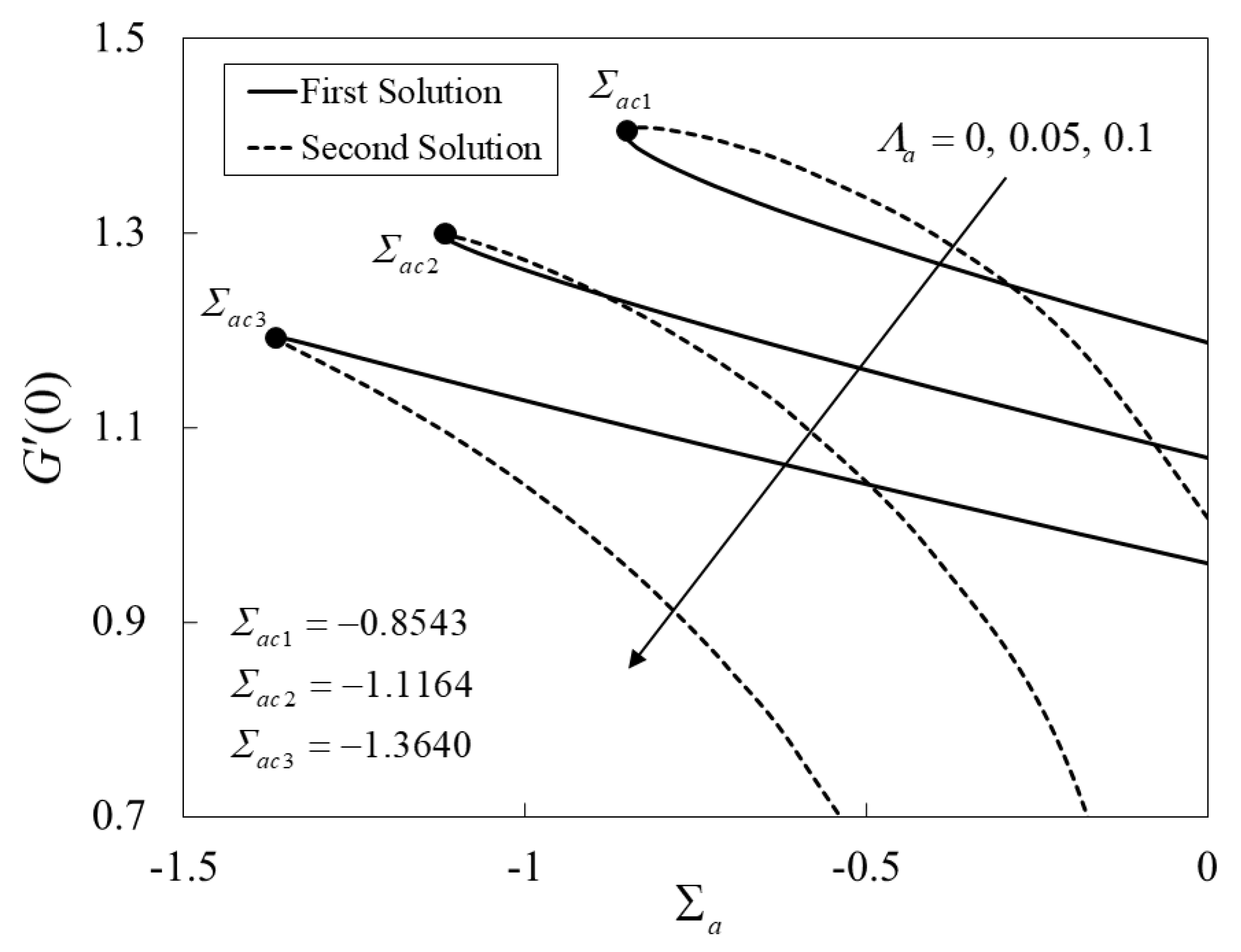
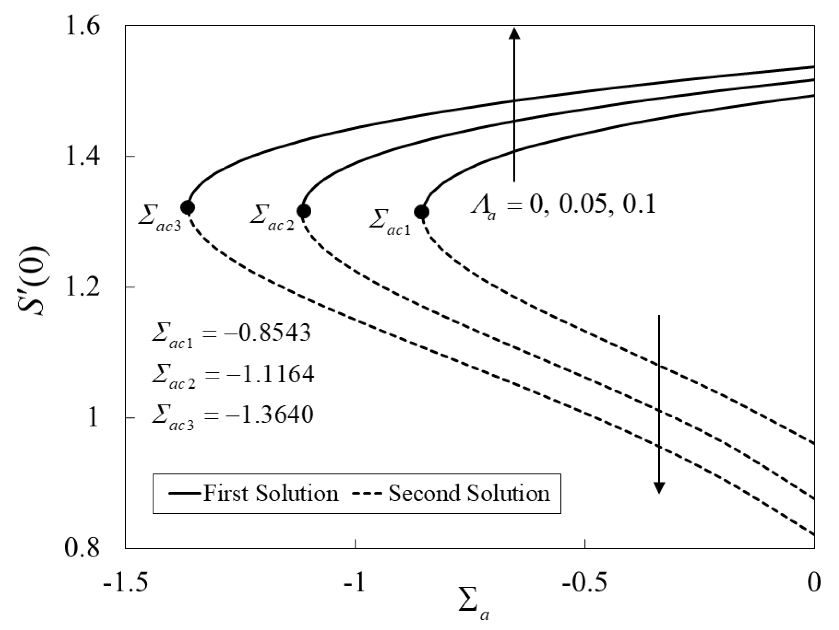
Figure 2, Figure 3 and Figure 4 elucidate the variation in the $C_f$, $N{u}_{x_r}$, and $S{h}_{x_r}$ due to the larger values of ${\mathsf{\Lambda }}_a$ against ${\mathsf{\Sigma }}_a$, respectively. Multiple branch (FBS and SBS) solutions are accomplished in all the physical quantities for the only case of the buoyancy opposing flow (${\mathsf{\Sigma }}_a<0$), while in the case of the buoyancy assisting flow (${\mathsf{\Sigma }}_a>0$), only a single solution is possible. Further, these graphs illustrate the values of $C_f$ and $S{h}_{x_r}$ increase for the FBS and decline for the SBS due to the larger impact of ${\mathsf{\Lambda }}_a$, while the $N{u}_{x_r}$ abruptly shrinks for both solution branches. In the physical scenario, the larger influence of the magnetic parameter ${\mathsf{\Lambda }}_a$ can create a strong drag force which shrinks the motion of the fluid flow of the hybrid nanoparticles. Therefore, the motion of the fluid flow is inversely related to the friction of the fluid. As a result, the shear stress upsurges because of the larger impacts of the magnetic parameter. Since multiple solutions are possible here only for the case of the buoyancy opposing flow (${\mathsf{\Sigma }}_a<0$) where the FBS represents the physically stable or trustworthy solution and the SBS corresponds to the unstable (not physically reliable) solution. Moreover, the unique solution is observed in these graphs for the case when ${\mathsf{\Sigma }}_a={\mathsf{\Sigma }}_{ac}$, no solution is seen for the case when ${\mathsf{\Sigma }}_a<{\mathsf{\Sigma }}_{ac}$, and the possible outcomes are detected for the case when ${\mathsf{\Sigma }}_a>{\mathsf{\Sigma }}_{ac}$. According to the graphs, it is observable that for each distinct value of ${\mathsf{\Lambda }}_a$, the following change critical values are found (see Figure 2, Figure 3 and Figure 4) and are written in each window of the graphs. These critical points are highlighted by the small solid balls that the readers can easily see. Meanwhile, the magnitude of the critical values is also enriched monotonically with growing values of ${\mathsf{\Lambda }}_a$. This tendency further demonstrates that the boundary layer separation diminishes due to the influences of the larger magnetic parameter.

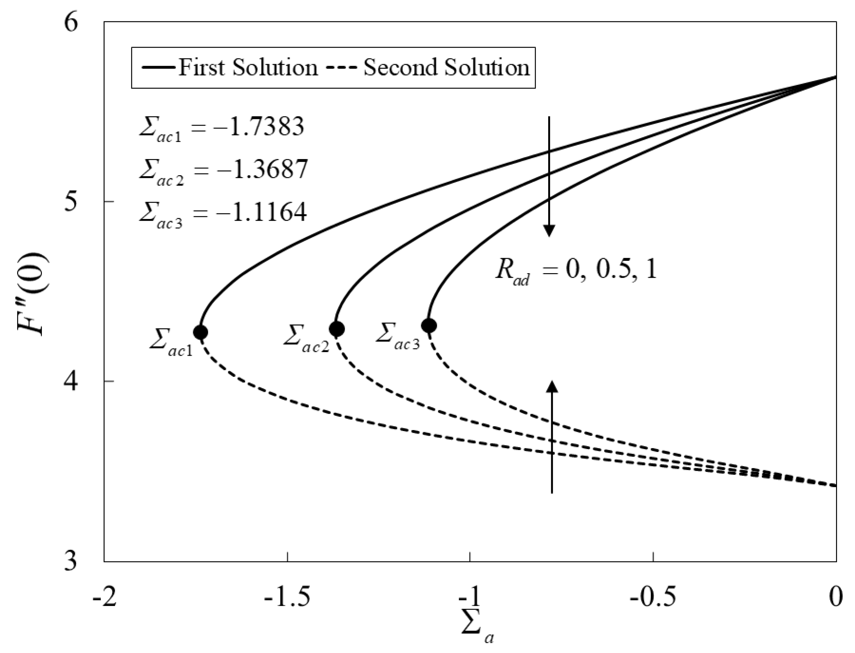
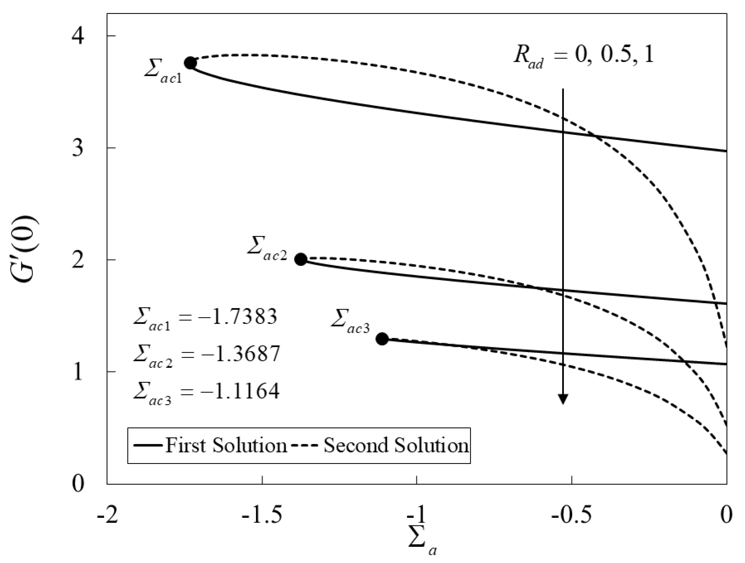
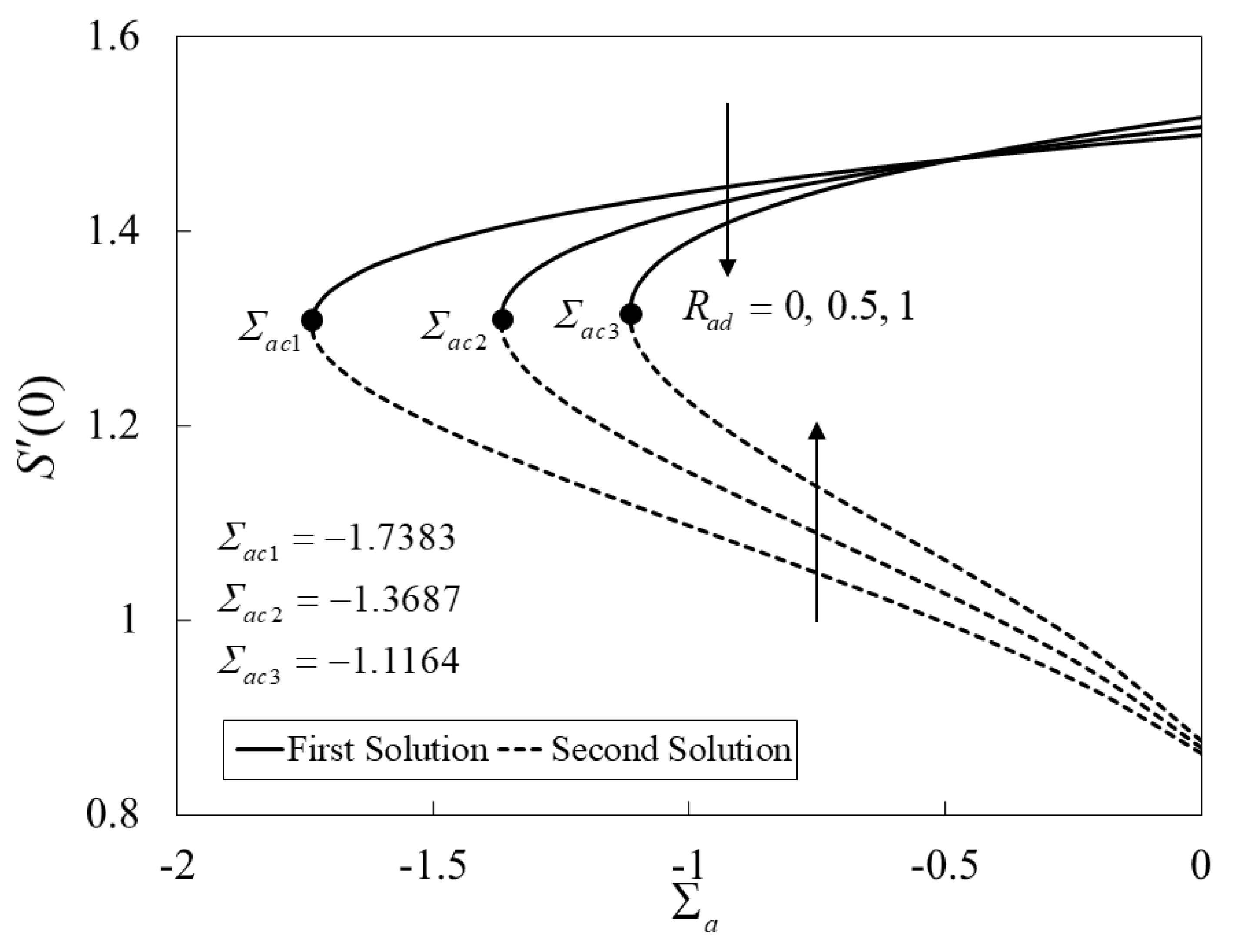
The impacts of the radiation parameter $R_{ad}$ on the physical quantities such as $C_f$, $N{u}_{x_r}$, and $S{h}_{x_r}$ of the (Ag-TiO₂/water) hybrid nanoparticles for the FBS as well as the SBS towards the buoyancy parameter ${\mathsf{\Sigma }}_a$ are graphically portrayed in Figure 5, Figure 6 and Figure 7. It is observed that the $C_f$ declines in the FBS but inclines in the SBS due to the augmentation in the values of $R_{ad}$, while $N{u}_{x_r}$ diminishes in the outcomes of the FBS as well as in the SBS due to the larger influence of the radiation parameter. In general, the larger impact of $R_{ad}$ gives a lower quantity of heating to the adjustable (Ag-TiO₂/water) hybrid nanofluid owing to the presence of the Eckert number in the similarity Equation (18). As a result, the heat transfer decelerates with the superior influences of $R_{ad}$. On the other hand,$S{h}_{x_r}$ initially improves for the FBS and then significantly starts decaying for the same branch as $R_{ad}$ increases. Meanwhile, the behavior of the solution continuously develop higher and higher for the SBS owing to the larger impressions of $R_{ad}$. For a particular domain of, unique solution is observed when, no solution when, and two solutions when. Moreover, the obtained critical values are ${\mathsf{\Sigma }}_{ac}=$ −1.7383, −1.3687, and −1.1164 for the corresponding dissimilar values of $R_{ad}$ (=0, 0.5 and 1.0), respectively. From these outputs, it can be seen that the behavior of the magnitude of the critical values decreases if we escalate the values of $R_{ad}$. Hence, the current pattern suggests that the separation of the boundary layer augments with larger values of $R_{ad}$.

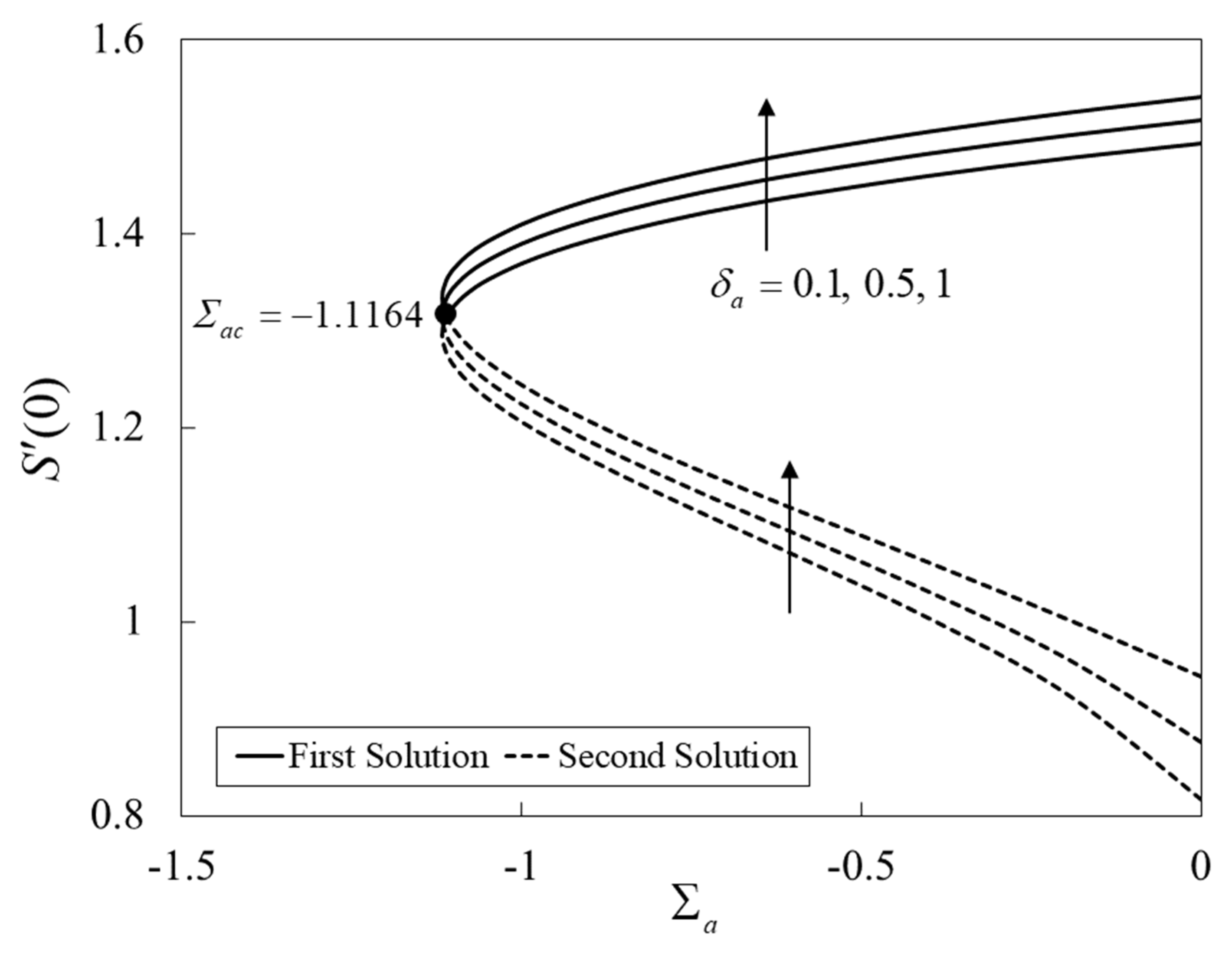
Figure 8 expounds the variations in the thermophoretic parameter ${\delta }_a$ on the local Sherwood number $S{h}_{x_r}$ of the (Ag-TiO₂/water) hybrid nanoparticles for both solution branches versus ${\mathsf{\Sigma }}_a$. For rising values of ${\delta }_a$, the mass transfer rate enriches for the FBS as well as for the SBS, while the gap between the outcomes looks similar in both branches with ${\delta }_a$. Generally, this behavior is due to the fact that higher consequences of the parameter ${\delta }_a$ can improve the thermophoretic coefficient $k$; as a result, the mass transfer rate would be significantly developed. Moreover, higher values of the thermophoretic parameter ${\delta }_a$ can give us a single bifurcation value as shown in the graph (see Figure 8).

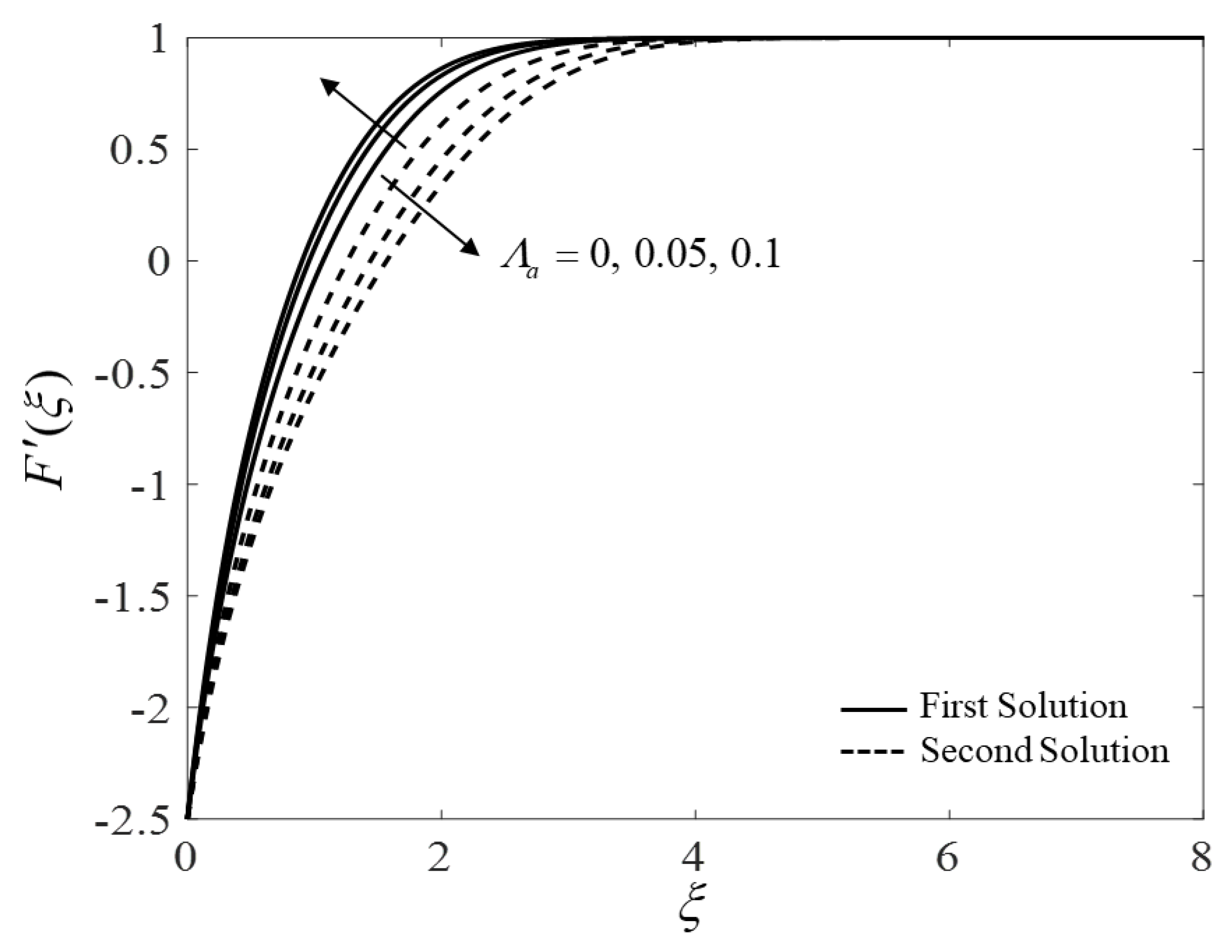
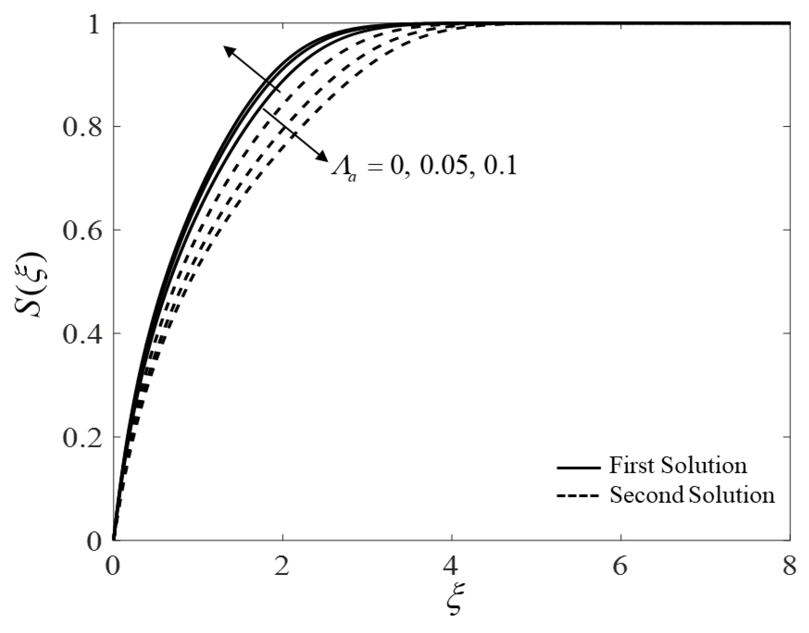
Figure 9, Figure 10 and Figure 11 display the variation in the $F{}^{\prime }\left(\xi \right)$, $G\left(\xi \right)$, and $S\left(\xi \right)$ of the (Ag-TiO₂/water) hybrid nanoparticles for the two dissimilar branch solutions due to the greater values of ${\mathsf{\Lambda }}_a$ against the pseudo-similarity parameter $\xi$, respectively. Further, to deal with these graphical outcomes, it is observed that the velocity and concentration distribution profiles increase for the FBS and falloffs the curves for the SBS due to the larger values of ${\mathsf{\Lambda }}_a$. Moreover, this dynamic growth of the (Ag-TiO₂/water) hybrid nanoparticles’ fluid flow for the FBS indicates that the velocity and concentration boundary layer become progressively thinner specifying that the magnetic parameter has a sensational influence and supports the motion of the hybrid nanoparticles near the surface of the thermophoretic flat plate. On the other hand, the temperature distribution behaves differently in both solution branches as compared to the outcomes of $F{}^{\prime }\left(\xi \right)$ and $S\left(\xi \right)$ for the larger impact of the magnetic parameter. As a general explanation, the larger magnetic parameter produces the conception of the Lorentz forces which creates a noticeable boost in the motion of the fluid and ultimately affects or decreases the temperature distribution.

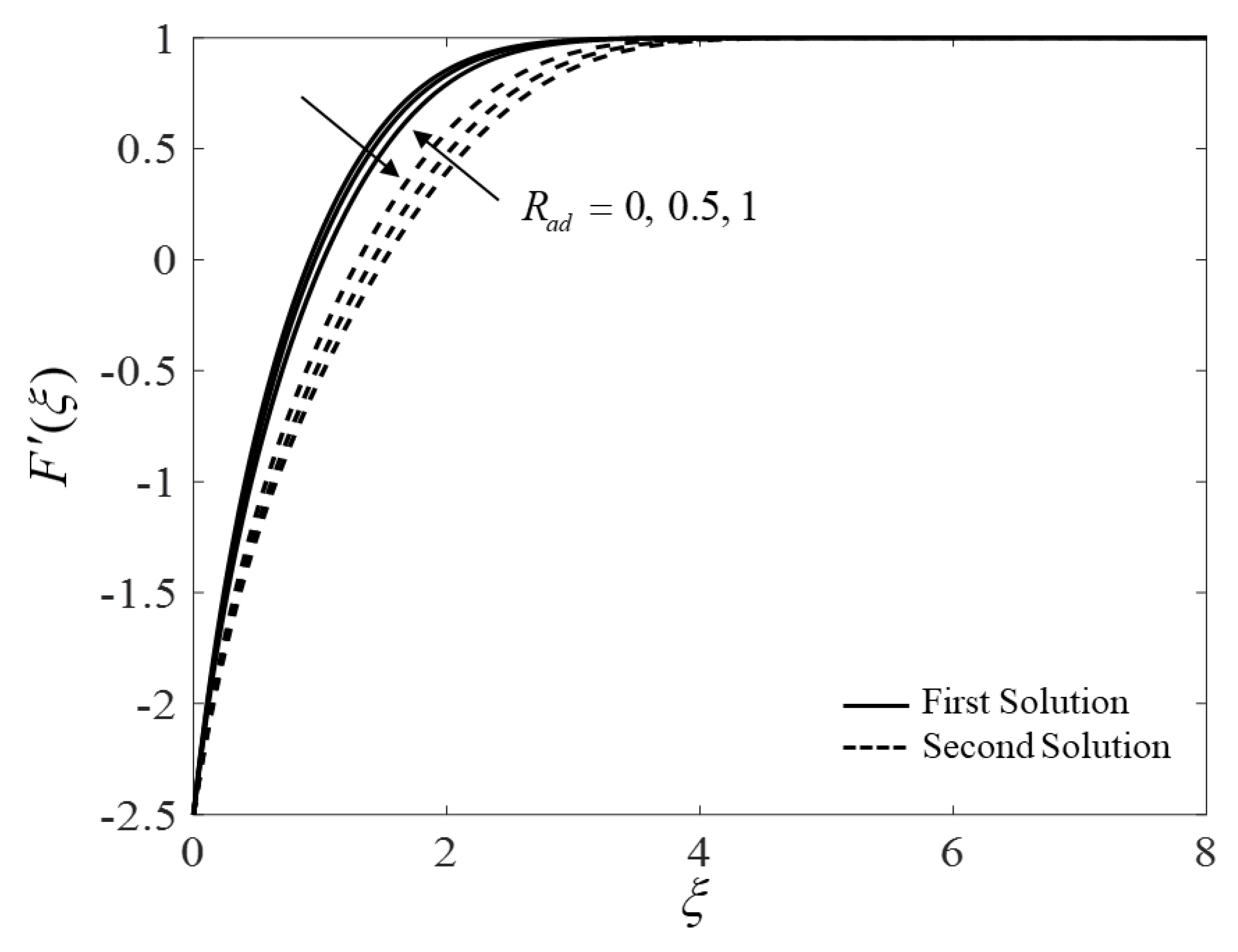
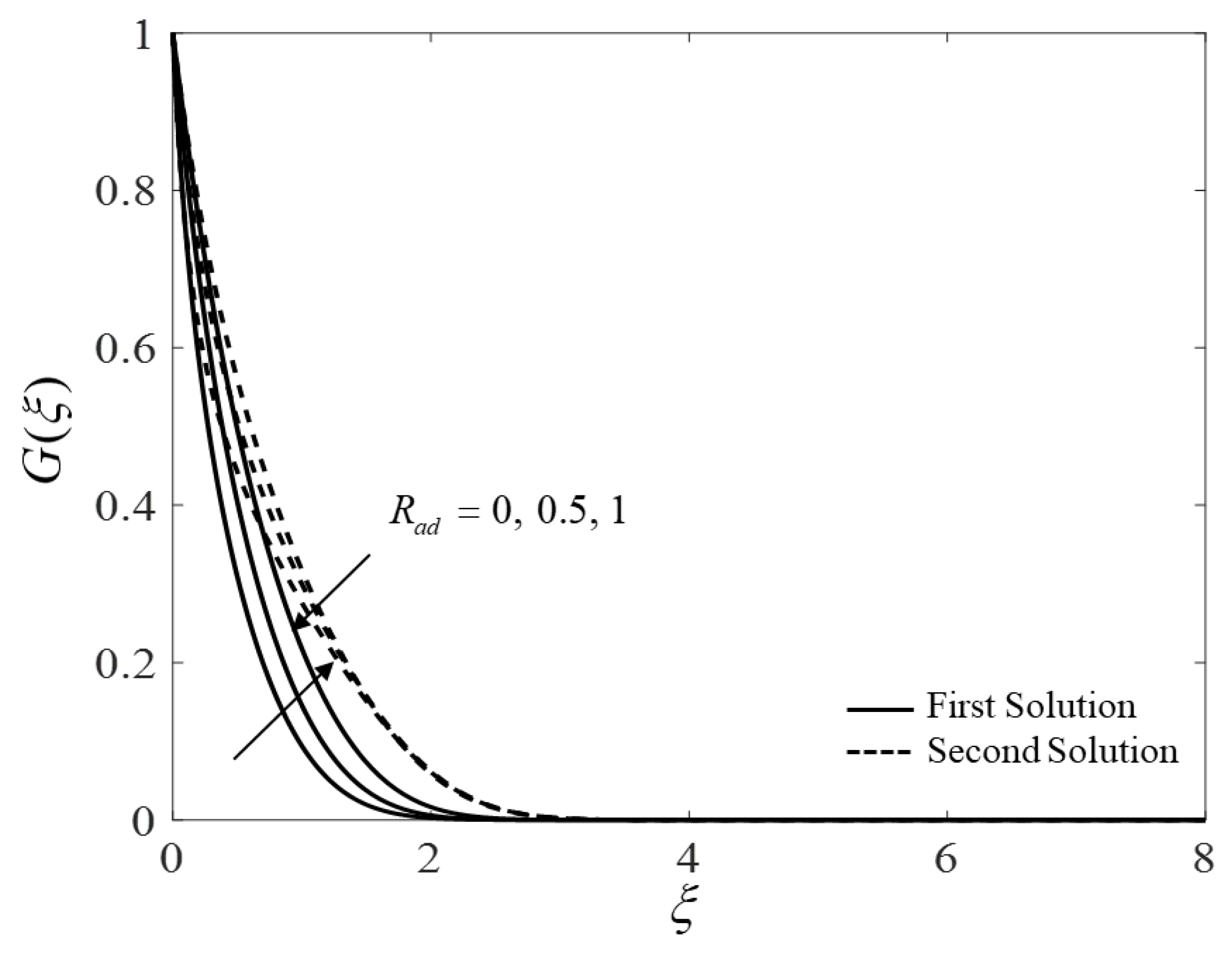
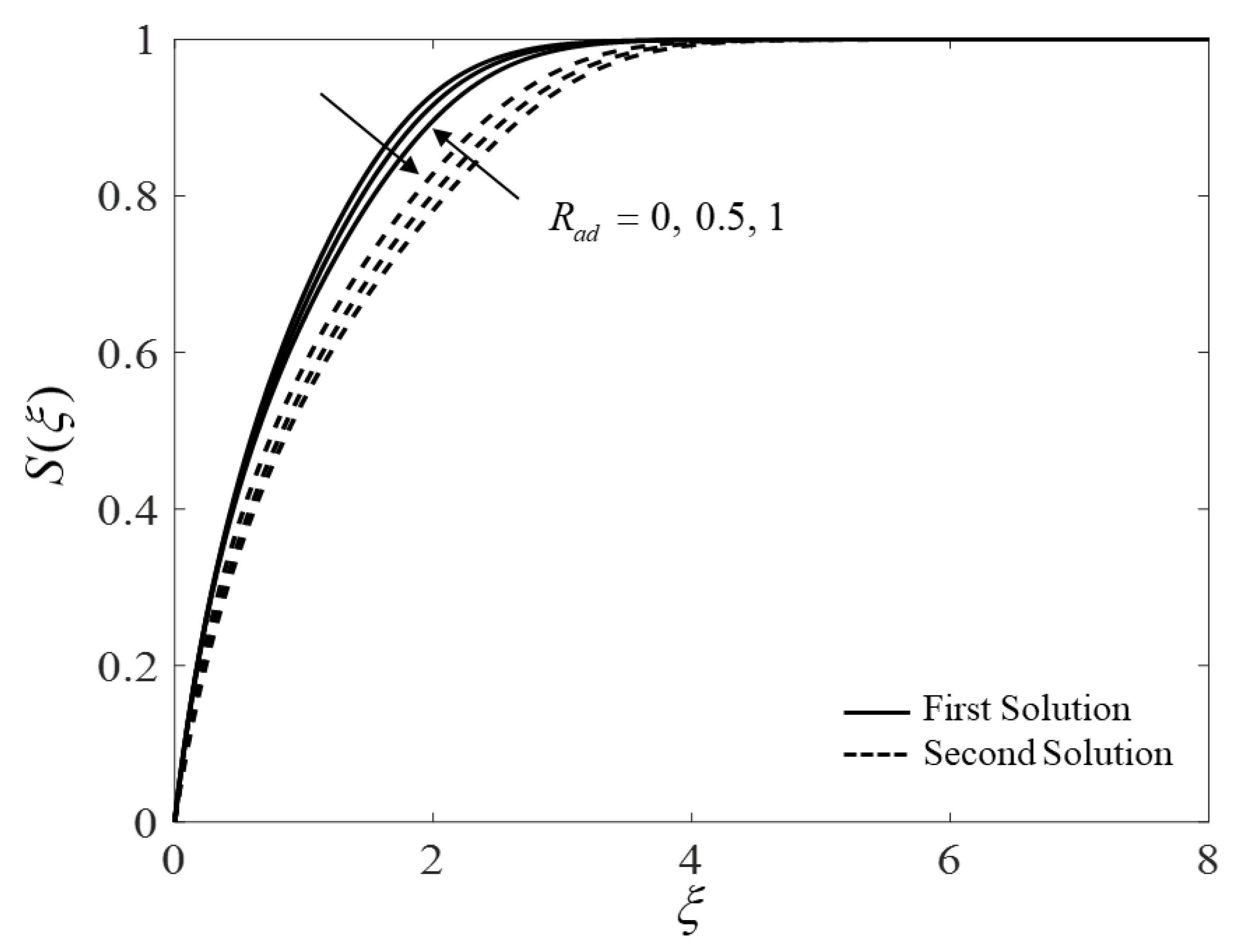
The impacts of the radiation parameter $R_{ad}$ on the profiles $F{}^{\prime }\left(\xi \right)$, $G\left(\xi \right)$, and $S\left(\xi \right)$ of the (Ag-TiO₂/water) hybrid nanoparticles for the FBS as well as for the SBS are graphically established in Figure 12, Figure 13 and Figure 14, respectively. The radiation parameter has a significant influence on the velocity, concentration, and temperature distributions. The rise in the radiation parameter accelerates the temperature but declines the fluid velocity and concentration for the FBS, while the tendency for the SBS is the opposite. Moreover, the thickness of the thermal boundary layer enriches with higher radiation parameters and with lower velocity or momentum and concentration boundary layers. Physically, the maximum impacts of radiation cause a considerable quantity of heating to the (Ag-TiO₂/water) hybrid nanoparticles that augments the temperature distribution as well as the thickness of the thermal boundary layer.

6. Conclusions

The impact of thermophoretic and radiative heat flux on MHD mixed convection water-based hybrid Ag-TiO₂ nanofluid flow over a permeable moving inclined flat plate with uniform free-stream velocity has been studied numerically. It has been found that for a specific set of embedded influential flow parameters, the shear stress, velocity profiles, heat transfer, temperature distribution profiles, concentration distribution, and the mass transfer reveal multiple (FBS and SBS) solutions over a broad range of the mixed or buoyancy convection parameter. The main findings are concluded as follows:

• The mass transfer and the shear stress enlarge owing to the higher magnetic parameter while the heat transfer reduces.
• Increasing the solid volume fraction of silver and titanium dioxide nanoparticles enhances the shear stress and mass transfer but reduces the heat transfer.
• The augmented value of the thermophoretic parameter develops the mass transfer while the heat transfer rate shrinks with Eckert number.
• The magnitude of the critical values surges due to the higher influences of the magnetic parameter but reduces with the radiation parameter.
• The higher influence of the thermophoretic parameter enriches the mass transfer rate.
• The boundary layer separation enhances with radiation, but shrinks owing to the Lorentz forces.
• The velocity and concentration decelerate with the radiation parameter, while the temperature significantly increases.