
A Boundary Element Procedure for 3D Electromagnetic Transmission Problems with Large Conductivity


1
Departamento de Matemáticas y Estadística, Universidad del Norte, Barranquilla 080007, Colombia
2
Department of Mathematics Sciences, Brunel University, London UB8 3PH, UK
3
Fakultät für Elektrotechnik Theoretische Elektrotechnik und Numerische, Helmut-Schmidt-Universität, 30167 Hamburg, Germany
*
Author to whom correspondence should be addressed.
Mathematics 2022, 10(7), 1148; https://doi.org/10.3390/math10071148
Submission received: 19 January 2022
/
Revised: 2 March 2022
/
Accepted: 6 March 2022
/
Published: 2 April 2022
(This article belongs to the Topic Engineering Mathematics)
Abstract
:We consider the scattering of time-periodic electromagnetic fields by metallic obstacles, or the eddy current problem. In this interface problem, different sets of Maxwell equations must be solved both in the obstacle and outside it, while the tangential components of both electric and magnetic fields are continuous across the interface. We describe an asymptotic procedure, applied for large conductivity, which reflects the skin effect in metals. The key to our method is a special integral equation procedure for the exterior boundary value problems corresponding to perfect conductors. The asymptotic procedure leads to a great reduction in complexity for the numerical solution, since it involves solving only the exterior boundary value problems. Furthermore, we introduce a FEM/BEM coupling procedure for the transmission problem and consider the implementation of Galerkin’s elements for the perfect conductor problem, and present numerical experiments.
1. Introduction
We present asymptotic expansions with respect to inverse powers of conductivity for the electrical and magnetic fields and report the algorithm of MacCamy and Stephan [1], which allows us to compute the expansion terms of the electrical field in the exterior domain by successively solving only exterior problems (so-called perfect conductor problems). We use various data for the interfaces between the conductors (metal) and the isolator (air). We solve the exterior problems numerically by applying the Galerkin boundary element method to boundary integral equations of the first kind, which were originally introduced by MacCamy and Stephan in [2]. This system of integral equations on the interface results from a single layer ansatz for the electrical field and has unknown densities, namely, a vector field and a scalar function on which we approximate with lower-order Raviart Thomas elements and continuous piecewise linear functions on a regular, triangular mesh on . As in the two dimensional case investigated by Hariharan [3,4] and MacCamy and Stephan [5], the asymptotic procedure gives for the computation of the solution of the transmission problem a great reduction in complexity, since it involves solving only the exterior problem, and furthermore, only a few expansion terms must be computed. We describe in detail how to implement the boundary element method for the perfect conductor problem. As an alternative to the asymptotic expansions for the solution of the transmission problem, we introduce a new finite element/boundary element Galerkin coupling procedure which converges quasi-optimally toward the energy norm.
2. Asymptotic Expansion for Large Conductivity and Skin Effect
Let be a bounded region in representing a metallic conductor and represent air. The parameters , , denoting permittivity, permeability and conductivity, are assumed to be zero in with positive , and values in . Let the incident electric and magnetic fields, and , satisfy Maxwell’s equations in air. The total fields and satisfy the same Maxwell’s equations as and in , but a different set of equations in . Across the interface , which is assumed to be a regular analytic surface, the tangential components of both and are continuous. and represent the scattered fields. All fields are time-harmonic with frequency . As in [1], we neglect conduction (displacement) currents in air (metal).
Problem : Given and , find and , such that
Here and are dimensionless parameters, and , if displacement currents are neglected in metal . The subscript T denotes a tangential component, and the superscripts plus and minus denote limits from and .
At higher frequencies, the constant is usually large, leading to the perfect conductor approximation. Formally this means solving only the equation and requiring that on . If we let and denote the scattered fields, we obtain
Problem : Given , find and , such that
Remark 1.
There exists at most one solution of problem for any and (see [8]).
Remark 2.
There exists a sequence , such that if , then curl, in , on Σ implies in .
We are interesting in an asymptotic expansion of the solution of problem with respect to inverse powers of conductivity. With denoting the distance from measured into along the normal to , the expansions reads:
Here and are independent of , which is proportional to . The exponential in (5) and (6) represents the skin effect. Next, we present from [1] these expansions for the half-space case where the various coefficients can be computed recursively. Note and in (3) and (4), respectively, are simply the perfect conductor approximation, that is, the solution of . and in (3) and (4) can be calculated successively by solving a sequence of problems of the same form as but with boundary values determined from earlier coefficients. The and in (5) and (6), respectively, are obtained by solving ordinary differential equations in the variable .
For the ease of the reader, we present here in the half-space case , i.e., , and , i.e., , a formal procedure to compute , , which was given by MacCamy and Stephan [1]. They substituted Equations (3)–(6) into for and equated coefficients of . Here, we give a short description of their approach.
Let and decompose field into tangential and normal components:
with orthogonal component , and unit vectors ().
Then, one computes with the surface gradient , the rotation
and
Now, by setting , one obtains for
and
Hence, matching coefficients of and , respectively, yields , and implying .
As coefficients of , one obtains
Now the gauge condition implies and ; hence and Thus, .
Setting
For , we have that yields
Matching coefficients of , one finds in
(and corresponding due to )
With the above relations, the recursion process goes as follows. First one use (6.10) for and (6.13), in [1], to conclude that
Now is just the solution of , which can be solved by the boundary integral equation procedure introduced in MacCamy and Stephan [1] and revisited below. However, from we obtain
Therefore, by (6.10), in [1], we have, again, a new solvable problem for which is just like , that is
but with new boundary values for as given by (18).
For the complete algorithm see [1]. Note, with , we have yielding in
A comparison with Peron’s results (see Chapter 5 in [9]) shows that , , in , and . Furthermore, we see that the first terms in the asymptotic expansion of the electrical field for a smooth surface derived by Peron coincide with those for the half-space investigated by MacCamy and Stephan, namely, , , .
Remark 3.
From Theorem 5 in Chapter 3 of [10], there exists only one solution to the electromagnetic transmission problem for a smooth interface. This solution which can be computed by the boundary integral equation procedure is shown below, where we assume that (19) holds. Then, for the electrical field obtained via the boundary integral equation system, we have that in the tubular region , there holds for the remainders obtained by truncating (3) and (5) at
for constants , independent of ρ.
3. A Boundary Integral Equation Method of the First Kind
Next, we describe the integral equation procedure for and from [1,7,11,12]. Throughout the section, we require that
These methods, like others, are based on the Stratton–Chu formulas from [6]. To describe these, some notation is needed. Let denote the exterior normal to . Given any vector field defined on , we have
where , which lies in the tangent plane, is the tangential component of .
Define the simple layer potential for density (correspondingly for a vector field) for the surface by
For a vector field on , define by (21) with replacing .
We collect in the following lemma some of the well-known results about the simple layer potential .
Remark 4
(Lemma 2.1 in [1]). For any complex κ, and any continuous ψ on Σ, there holds:
- (i)
- is continuous in ,
- (ii)
- in ,
- (iii)
- as ,
- (iv)
- where as .
- (v)
- where the matrix function satisfies as .
For problem in , the Stratton–Chu formula gives
Similarly, for problem , in
For given , and , (23) yields a solution of . However, we know only . The standard treatment of starts from (23), sets and and replaces with an unknown tangential field yielding
Then the boundary condition yields an integral equation of the second kind for in the tangent space to .
The method (24) is analogous to solving the Dirichlet problem for the scalar Helmholtz equation with a double layer potential. However, having found , it is hard to determine , or equivalently , on . Note that calculating on involves finding a second normal derivative of .
The method in [1] for is analogous to solving the scalar problems with a simple layer potential (see [13]). MacCamy and Stephan use (23), but this time they set and replace and by unknowns and M. Thus, they take
If they can determine , then in this case, they can use Remark 4 to determine ; hence, on .
With the surface gradient on , the boundary conditions in (1) and (25) imply, by continuity of ,
or equivalently,
Note that for any field defined in a neighborhood of , one can define the surface divergence by
As shown in [1]), there holds, for any differentiable tangential field , that
4. FEM/BEM Coupling
Next, we present a coupling method for the interface problem (see [10,14,15,16,17]). Integration by parts gives in for the first equation in , with ,
Therefore, with and setting in , we obtain
Note that , where is a smoothing operator.
As shown in (Lemma 4.5 in [1]), there exists a continuous map from into , for any real number r with
As shown in [2], the system of boundary operators on (which is equivalent to (26) and (27)),
is strongly elliptic as a mapping from into , where denote the surface gradient (surface divergence) and the Laplace–Beltrami operator on .
Now, the fem/bem coupling method is based on the variational formulation: For given incident field on , find , and with
, , .
In order to formulate a conforming Galerkin scheme for (31), take subspaces , , with the mesh parameter h and look for , , such that
where is the operator given by the left-hand side in (31), .
Theorem 1.
Proof.
First, note that system (31) is strongly elliptic in , which follows by considering as a system of pseudodifferential operators (cf. [2]). The only difference from [2], is that here we additionally have the first equation in (31). Since , by taking , the principal symbol of has the form (with )
where and is perpendicular to .
Obviously the two sub-blocks are strongly elliptic (see [2] for the lower sub-block). Assuming that is not an eigenvalue of , we have existence and uniqueness of the exact solution. Due to the strong ellipticity of , there exists a unique Galerkin solution and the a priori error estimate holds, due to the abstract results by Stephan and Wendland [18]. □
5. Galerkin Procedure for the Perfect Conductor Problem ()
Next, we present implementations of the Galerkin methods (see [7,10,19,20]) and some numerical experiments for the integral equations (26) and (27). These experiments were performed with the package Maiprogs (cf. Maischak [21,22]), which is a Fortran-based program package utilized for finite element and boundary element simulations [23]. Initially developed by M. Maischak, Maiprogs has been extended for electromagnetic problems by Teltscher [24] and Leydecker [25].
We investigate the exterior problem by performing the integral equations procedure with (26) and (27):
Partial integration in the second term of
shows that the formulation (35) is symmetric: by definition of symmetric bilinear forms a and c, of the bilinear form b and linear form ℓ through
the variational formulation has the form: find such that
for all .
We now work with finite dimensional subspaces of dimension n and of dimension m, and seek approximations and for and M, such that
for all and .
Let be a basis of and be a basis of . , and are of the forms
We have considered a basis of and a basis of . These functions were chosen as piecewise polynomials. To obtain these bases, we considered suitable basis functions locally on the element of a grid, i.e., on each component grid.
Start from a grid
with N elements, and let and be the basis of a square reference element . The local basis functions on an element are each or .
Therefore, we should calculate first
where or are the basis functions of and
Test each local basis function against any other local basis function and sum the result to the test value of the global basis functions, which include these local basis functions.
Let be the index set for the grid elements, the index set for the basic functions on the reference element and the index set for the global basis functions.
Let be the mapping from local to global basis functions, such that , if the local basis function component of the global basis function is .
Let be the set of all pairs of with ; then,
We are dealing in this implementation with Raviart–Thomas basis functions. The transformation of these functions requires a Peano transformation . Thus, if , is calculated by , then the Peano transformation of the local basis functions to the basic functions on the reference element then gives
with and , and referent element .
The calculation of the integrals with Helmholtz kernel is not exact. We consider the expansion of the Helmholtz kernel in a Taylor series. There holds
The first terms are singular for , and their corresponding integrals are treated by analytic evaluation in Maiprogs (cf. Maischak [21,22,26]), but the integrals of all other terms can be calculated with sufficient accuracy by Gaussian quadrature.
Compute
with described above, and , the analogously defined map for the basic functions of .
While a transformation of the scalar basis functions is not required, the transformation of the surface divergence of Raviart–Thomas elements is carried out by and we have
with and . The calculation of is similar to the one mentioned before.
The calculation of the right-hand side appears simple at first glance, since there are no single layer potential terms. However, the right-hand side must be computed by quadrature.
The quadrature of an integral over on the reference element is determined by the quadrature points , and the associated weights , which are processed in x and y directions. Perform the two-dimensional quadrature as a combination of one-dimensional quadratures in each x and y direction, and use here the weights from the already implemented one-dimensional quadrature formula. With quadrature points in x-direction and quadrature points in y-direction, the quadrature formula reads:
The quadrature points on the square reference element and the corresponding weights for Gaussian quadrature were implemented in Maiprogs already. For triangular elements, use a Duffy transformation.
We will now calculate the right-hand side in the Galerkin formulation, i.e., the linear form ℓ, applied to the base functions , . The quadrature takes place on the reference element. Decompose global functions into local basis functions and then use the Peano transformation for the Raviart–Thomas functions. Therefore,
with . Applying (45) with , leads to
with . As before, the task is carried out by looping through all grid components, and the values are added to the entries for each of its base function.
The electrical field can be calculated by
We have for the first term in (47) with
Then using Peano transformation, it follows that
For the second term in (47), one gets
The calculation of is done as follows (compare Remark 4).
6. Numerical Experiments
Here, consider one example to test the implementation. As the domain, take the cube . We tested the Galerkin method in (37). We chose the wave number (or ) and the exact solution
and
where denotes the outer normal vector at a point on the surface . We can write each term of Equation (26) as:
and
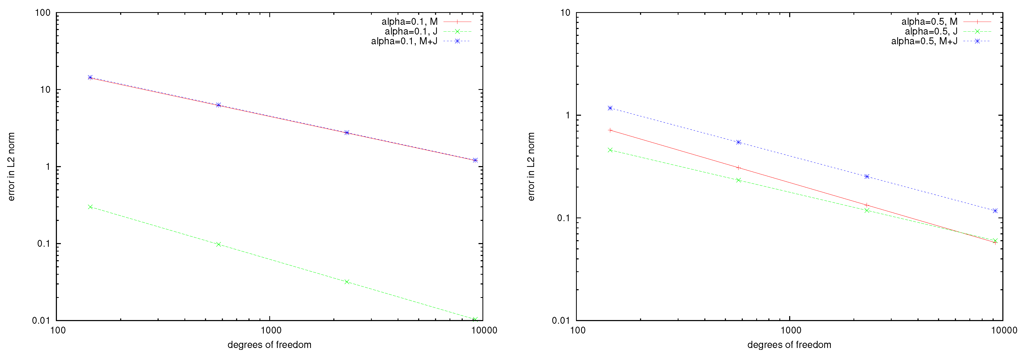
We used different values of for our investigation. In Table 1, we present the results of the errors in energy norm and -norm for for the uniform h version with polynomial degree . In Figure 1 and Figure 2, we compare the h-version with different . The exact norm, known by extrapolation, for is , for is , and for is . Here, and (see [27]). The exact -norms, known by extrapolation, for are and ; for are and ; and for are and .
The convergence rates , for are, for the energy norm , and for the -norm and . With , the energy norm of , the -norms of and and , for the energy norm , and for -norm and .
Let us compare the numerical convergence rates above for the boundary element methods obtained in the above example with the theoretical convergence rates predicted by Theorem 1. Note that we have implemented the boundary integral equation system (26), and (27) and note the strongly elliptic system (30), where convergence is guaranteed due to Theorem 1. Nevertheless, our experiments show convergence for the boundary element solution, but with suboptimal convergence rates. Theorem 1 predicts (when Raviart–Thomas elements are used to approximate and piecewise linear elements to approximate M) a convergence rate of order in the energy norm for smooth solutions and M. Our computations depend on the parameter which is a well-known effect with boundary integral equations where it may come to spurious eigenvalues diminishing the orders of the Galerkin approximations. Due to the cube , the numerical solution might become singular near the edges and corners of ; hence, the Galerkin scheme converges sub-optimally.
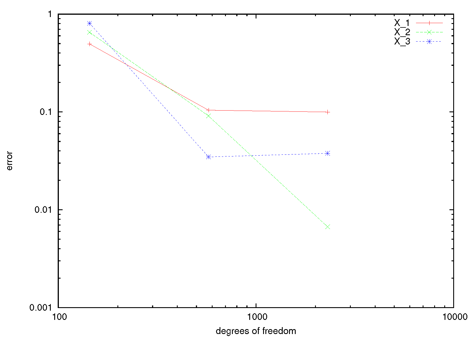
Next, we applied the boundary element method above to compute the first terms in the asymptotic expansion of the electrical field considered in Section 1 (Remark 1). In this way we obtained good results for the electrical field at some point away from the transmission surface by only computing a few terms in the expansion.
Algorithm for the asymptotic of the eddy current problem:
7. Conclusions
In this article we have studied the scattering of time-periodic electromagnetic fields by metallic obstacles, or the eddy current problem. An asymptotic procedure was described, applied for large conductivity, and reflects the skin effect in metals. A special integral equation procedure was introduced for the exterior boundary value problems corresponding to perfect conductors. In addition, an FEM/BEM coupling procedure was presented for the transmission problem, and the implementation of Galerkin’s elements was considered for the perfect conductor problem. The numerical experimentation showed good behavior by the procedure.
Author Contributions
J.E.O.P., M.M. and Z.N. contributed equally on the development of the theory and their respective analysis. All authors have read and agreed to the published version of the manuscript.
Funding
This research was supported in part by the ALECOL-DAAD Program and COLCIENCIAS through contract number CT 793-2013, and code 1215-569-33876.
Institutional Review Board Statement
Not applicable.
Informed Consent Statement
Not applicable.
Data Availability Statement
Not applicable.
Acknowledgments
This research was supported in part by the ALECOL-DAAD Program and COLCIENCIAS through contract number CT 793-2013, and code 1215-569-33876. Institute for Applied Mathematics, Leibniz University of Hannover, Hannover-Germany, Department of Mathematics Sciences, Brunel University, UK and Universidad del Norte, Barranquilla-Colombia. Furthermore, we thank the anonymous referees for their suggestions.
Conflicts of Interest
The authors declares that there is no conflict of interest regarding the publication of this paper.
References
- MacCamy, R.C.; Stephan, E.P. Solution procedures for three-dimensional eddy current problems. J. Math. Anal. Appl. 1984, 101, 348–379. [Google Scholar] [CrossRef] [Green Version]
- MacCamy, R.C.; Stephan, E.P. A boundary element method for an exterior problem for three-dimensional Maxwell’s equations. Appl. Anal. 1983, 16, 141–163. [Google Scholar] [CrossRef]
- Hariharan, S.I.; MacCamy, R.C. Low frequency acoustic and electromagnetic scattering. Appl. Numer. Math. 1986, 2, 29–35. [Google Scholar] [CrossRef] [Green Version]
- Hariharan, S.I.; MacCamy, R.C. Integral equation procedures for eddy current problems. J. Comput. Phys. 1982, 45, 80–99. [Google Scholar] [CrossRef]
- MacCamy, R.C.; Stephan, E.P. A skin effect aproximation for eddy current problems. Arch. Ration. Mech. Anal. 1985, 90, 87–98. [Google Scholar] [CrossRef]
- Stratton, J.A. Electromagnetic Theory; Mc Graw-Hill: New York, NY, USA, 1941. [Google Scholar]
- Weggler, L. Stabilized boundary element methods for low-frequency electromagnetic scattering. Math. Methods Appl. Sci. 2012, 35, 574–597. [Google Scholar] [CrossRef]
- Müller, C. Fundations of Mathematical Theory of Electromagnetic Waves; Springer: New York, NY, USA, 1969. [Google Scholar]
- Peron, V. Modélisation Mathématique de Phénomènes Électromagnétiques dans des Matériaux à Fort Contraste. Ph.D. Thesis, Université de Rennes I, Rennes, France, 2009. [Google Scholar]
- Ospino Portillo Jorge, E. Finite Elements/Boundary Elements for Electromagnetic Interface Problems, Especially the Skin Effect. Ph.D. Thesis, Institut of Applied Mathematics, Hannover University, Hannover, Germany, 2011. [Google Scholar]
- Lei, W.D.; Li, H.J.; Qin, X.F.; Chen, R.; Ji, D.F. Dynamics-based analytical solutions to singular integrals for elastodynamics by time domain boundary element method. Appl. Math. Model. 2018, 56, 612–625. [Google Scholar] [CrossRef]
- Xie, G.Z.; Zhong, Y.D.; Li, H.; Hao, B.; Du, W.L.; Sun, C.Y.; Wang, H.Q.; Wen, X.Y.; Wang, L.W. A systematic derived sinh based metod for singular and nearly singular boundary integrals. Eng. Anal. Bound. Elem. 2021, 123, 147–153. [Google Scholar] [CrossRef]
- Hsiao, G.; MacCamy, R.C. Solution of boundary value problems by integral equations of the first kind. SIAM Rev. 1973, 15, 687–705. [Google Scholar] [CrossRef]
- Ammari, H.; Nédxexlec, J.C. Couplage éléments finis équations intégrales puor la résolution des équations de Maxwell en milieu hétérogène. Équations aux dérivées partielles et applications. In Social Science & Médicine; Gauthier-Villars, H., Ed.; Elsevier: Paris, France, 1998; pp. 19–33. [Google Scholar]
- Ammari, H.; Nédxexlec, J.C. Coupling of finite and boundary element methods for the timeharmonic Maxwell equations II. A symmetric formulation. In The Maz’ya Anniversary Collection: Volume 2 (Rostock, 1998), Volume 110 of Operator Theory: Advances and Applications; Birkhäuser: Basel, Switzerland, 1999; pp. 23–32. [Google Scholar]
- Hitmair, R. Symmetric coupling for eddy current problems. SIAM J. Numer. Anal. 2002, 40, 41–65. [Google Scholar] [CrossRef] [Green Version]
- Hitmair, R. Coupling of finite elements and boundary elements in electromagnetic scattering. SIAM J. Numer. Anal. 2003, 41, 919–944. [Google Scholar] [CrossRef] [Green Version]
- Stephan, E.P.; Wendland, W.L. Remars to Galerkin and least squares methods with finite elements for general elliptic problems. Manuscripta Geod. 1976, 1, 93–123. [Google Scholar]
- Christiansen, S. Mixed Boundary Element Method for Eddy Current Problems; Research Report 2002-16; SAM-ETH Zürich: Zürich, Switzerland, 2002. [Google Scholar]
- Taskinen, M.; Vänskxax, S. Current and charge integral equation formulations and picards extended maxwell system. IEEE Trans. Antennas Propag. 2007, 55, 3495–3503. [Google Scholar] [CrossRef]
- Maischak, M. Manual of the Sotfware Package Maiprogs; Institut of Applied Mathematics, Hannover University: Hannover, Germany, 2007. [Google Scholar]
- Maischak, M. Book of Numerical Experiments (B.O.N.E.); Institute for Applied Mathematics, University of Hannover: Hannover, Germany, 2010. [Google Scholar]
- Maischak, M. Technical Manual of the Program System Maiprogs; Institut of Applied Mathematics, Hannover University: Hannover, Germany, 2010. [Google Scholar]
- Teltscher, M. A Posteriori Fehlerschätzer für Elektromagnetische Kopplungprobleme in Drei Dimensionen. Ph.D. Thesis, Institut of Applied Mathematics, Hannover University, Hannover, Germany, 2002. [Google Scholar]
- Leydecker, F. hp-Version of the Boundary Element Method for Electromagnetic Problems-Error Analysis, Adaptivity, Preconditioners. Ph.D. Thesis, Institut of Applied Mathematics, Hannover University, Hannover, Germany, 2006. [Google Scholar]
- Maischak, M. The Analytical Computation of the Galerkin Elements for the Laplace, Lamé and Helmholtz Equation in 3D-BEM; Institute for Applied Mathematics, University of Hannover: Hannover, Germany, 2000. [Google Scholar]
- Holm, H.; Maischak, M.; Stephan, E.P. The hp-Version of the boundary element method for Helmholtz screen problems. Computing 1996, 57, 105–134. [Google Scholar] [CrossRef]
Figure 1.
Errors in the L2-norm for .

Figure 2.
Errors in the L2-norm for and the energy norm for .

Figure 3.
Errors for the electrical field with respect to the degrees of freedom for , , and .


Table 1.
Errors in -norm and energy norm with respect to the degrees of freedom for .
| N | DOF | ||||||
|---|---|---|---|---|---|---|---|
| 1 | 144 | 8.502965 | 1.153119 | 2.085189 | 80.704374 | 0.299829 | 14.08929 |
| 2 | 576 | 8.568451 | 0.460150 | 2.104369 | 81.690279 | 0.097681 | 6.196968 |
| 3 | 2304 | 8.578833 | 0.033717 | 2.106395 | 81.879637 | 0.031823 | 2.725645 |
| 4 | 9216 | 8.654072 | 0.073274 | 2.117002 | 83.123825 | 0.010367 | 1.198835 |
| 1 | 144 | 1.603519 | 0.209552 | 2.149511 | 3.8937090 | 0.458159 | 0.714952 |
| 2 | 576 | 1.614451 | 0.093436 | 2.185426 | 3.9467491 | 0.232851 | 0.308704 |
| 3 | 2304 | 1.616616 | 0.041661 | 2.194608 | 3.9565591 | 0.118342 | 0.133293 |
| 4 | 9216 | 1.617260 | 0.018576 | 2.198619 | 3.9592220 | 0.060145 | 0.057554 |
| 1 | 144 | 1.774450 | 0.326497 | 2.350909 | 0.7243729 | 0.387707 | 0.279375 |
| 2 | 576 | 1.800799 | 0.111334 | 2.365011 | 0.7422644 | 0.343627 | 0.227618 |
| 3 | 2304 | 1.803838 | 0.037965 | 2.382843 | 0.7539064 | 0.304558 | 0.185450 |
| 4 | 9216 | 1.804284 | 0.012946 | 2.397906 | 0.7909461 | 0.269932 | 0.151093 |
Table 2.
Errors for electrical field in , , and .
| DOF | |||
|---|---|---|---|
| 144 | 0.4959 | 0.6499 | 0.8049 |
| 576 | 0.1043 | 0.0910 | 0.0347 |
| 2304 | 0.0998 | 0.0067 | 0.0378 |
Publisher’s Note: MDPI stays neutral with regard to jurisdictional claims in published maps and institutional affiliations. |
© 2022 by the authors. Licensee MDPI, Basel, Switzerland. This article is an open access article distributed under the terms and conditions of the Creative Commons Attribution (CC BY) license (https://creativecommons.org/licenses/by/4.0/).
Share and Cite
MDPI and ACS Style
Ospino Portillo, J.E.; Maischak, M.; Nezhi, Z. A Boundary Element Procedure for 3D Electromagnetic Transmission Problems with Large Conductivity. Mathematics 2022, 10, 1148. https://doi.org/10.3390/math10071148
AMA Style
Ospino Portillo JE, Maischak M, Nezhi Z. A Boundary Element Procedure for 3D Electromagnetic Transmission Problems with Large Conductivity. Mathematics. 2022; 10(7):1148. https://doi.org/10.3390/math10071148
Chicago/Turabian StyleOspino Portillo, Jorge Eliécer, Matthias Maischak, and Zouhair Nezhi. 2022. "A Boundary Element Procedure for 3D Electromagnetic Transmission Problems with Large Conductivity" Mathematics 10, no. 7: 1148. https://doi.org/10.3390/math10071148
Note that from the first issue of 2016, this journal uses article numbers instead of page numbers. See further details here.