A Dynamic Mechanistic Model of Perceptual Binding

Abstract

The brain’s ability to create a unified conscious representation of an object by integrating information from multiple perception pathways is called perceptual binding. Binding is crucial for normal cognitive function. Some perceptual binding errors and disorders have been linked to certain neurological conditions, brain lesions, and conditions that give rise to illusory conjunctions. However, the mechanism of perceptual binding remains elusive. Here, I present a computational model of binding using two sets of coupled oscillatory processes that are assumed to occur in response to two different percepts. I use the model to study the dynamic behavior of coupled processes to characterize how these processes can modulate each other and reach a temporal synchrony. I identify different oscillatory dynamic regimes that depend on coupling mechanisms and parameter values. The model can also discriminate different combinations of initial inputs that are set by initial states of coupled processes. Decoding brain signals that are formed through perceptual binding is a challenging task, but my modeling results demonstrate how crosstalk between two systems of processes can possibly modulate their outputs. Therefore, my mechanistic model can help one gain a better understanding of how crosstalk between perception pathways can affect the dynamic behavior of the systems that involve perceptual binding.

1. Introduction

Perceptual binding provides a unified conscious representation of an object that is described by several different perceptual features such as the object’s shape, color, and location [1,2]. Importantly, accumulated empirical evidence suggests that binding is critical for normal cognitive operation. Binding disorder occurs in damaged brains when patients cannot perceive more than one object at a time, have dissociations between different perception pathways, and have problems solving a discrimination task according to different percepts [3,4]. ‘Split-brain’ studies report the loss of interhemispheric integration and the functional disengagement of the right and left hemispheres with respect to cognitive activities [5,6]. Specifically, the independence of the two visual half-fields has been reported in patients with a complete transection of the corpus callosum [5]. Pictures of objects seen in one half of visual field (processed in one hemisphere) are dissociated in perception and memory from pictures seen in the other half-field (processed in the other hemisphere). Moreover, illusory conjunctions are often referred to as examples of binding errors [7,8]. Thus, a normal cognitive operation requires appropriate integration of neural signals from different perception pathways.

The concept of binding is often used to explain the integration of information across different sensory modalities into unified percepts [9]. Multisensory integration depends on the temporal relationship of the different sensory inputs and occurs only within the specific time window known as the ‘temporal binding window’ [10,11]. Several studies have shown, for example, that binding depends on the temporal arrangement of the stimulus sets [12] and that the temporal binding window varies in elderly and young adults [13,14,15,16]. Furthermore, cross-modal perceptual interaction studies have shown that sensory modalities (e.g., visual perception or direction of motion perception) can be altered by other modalities (e.g., sound) [17,18,19]. Such cross-modal interactions also occur within a specific temporal window, ~100 ms, that is comparable with the integration window of polysensory neurons in the mammalian brain [17].

Binding is also closely connected to the philosophical problem of the ‘unity of consciousness’ [20,21]. Consciousness-related binding is seen as the neural mechanism that maps the subjective phenomenal experiences in consciousness onto corresponding neural processes in the brain [21]. Thus, binding is a mechanism that phenomenally unifies entities constructed through multiple sensory modalities. It is remarkable that our conscious experience is unified even when the corresponding neural pathways that process different phenomenal contents are distributed all around the cortex [22].

Building binding models could help us better understand how our brain integrates information from different perception pathways to provide us with a unified and coherent conscious experience. Several models have been proposed to explain the mechanism of perceptual binding, among which the most frequently discussed is based on the neuronal synchrony or temporal correlation hypothesis [2,23,24,25]. In operational architectonics, an operational synchrony among neuronal processes initiated in different brain regions is postulated to play a central role in binding spatially dispersed phenomenal features into a unified phenomenal object [26,27,28]. A temporal alignment that permits binding between a stimulus and ongoing spontaneous neural activity is a core assumption of the temporo-spatial theory of consciousness [29,30]. Furthermore, an interdependence between information integration and consciousness has been postulated in several theories of consciousness [31,32,33,34]. For example, the integrated information theory identifies consciousness as the ability of the neuronal system to integrate information to the level at which information is consciously accessible [35,36,37]. In addition, some attempts to give a computational explanation of binding have been made within the framework of classical neural networks [2]. However, much remains to be understood about the neuronal processes involved in perceptual binding. Moreover, many works have been devoted to provide a critical evaluation of the temporal synchrony hypothesis as well as arguments against the existence of the binding problem in principle [38,39,40].

In this work, I present a mathematical model of binding, which is based on my previous model of oscillatory processes, that exhibits the dynamic behavior isomorphic to a specific percept [41,42,43]. The underlying concept of the approach has been described in Kraikivski, 2017 [43]. A mathematical formulation of a system of processes representing a percept isomorphic to the space has been elaborated in Kraikivski, 2020 [41]. The corresponding stochastic model to study implications of noise on the system of processes has been presented in Kraikivski, 2021 [42]. To study the binding mechanism, here I use two systems of oscillatory processes that are bound via negative feedback loops. Two different binding interaction wiring schemes are analyzed. I study how the sets of oscillatory processes modulate each other to identify different regimes of modulated oscillations, which are then represented in a two-parameter bifurcation diagram. Furthermore, I investigate how the system in these different regimes are capable of distinguishing different combinations of initial inputs (stimuli). I intend my dynamic model to help us understand how a possible mechanism of perceptual binding can be deduced from observable oscillating signals.

2. Model and Methods

Perceptual experiences of two individuals can be synchronized by the same stimulus; therefore, in principle, temporally correlated neuronal signals can be recorded in two non-interacting brains. In that case, however, the temporal synchronization is not sufficient to provide a unified conscious representation since the stimulus is still independently processed by each individual. Moreover, as discussed in the introduction, the functional disengagement of the right and left hemispheres with respect to cognitive activities has been reported in subjects with a complete transection of the corpus callosum which results in the loss of interhemispheric integration [5,6]. Such split-brain studies have revealed a lack of integration between the contents of the patient’s conscious states. Therefore, binding can occur only if there is a crosstalk between perception pathways that can interact and exchange information. Binding is thus detectable since the crosstalk between pathways may result in modulation and superposition of signals that can be analyzed. Here, I assume that direct interaction among perception pathways or corresponding processes is a necessary condition for binding, which can, in turn, induce temporal correlation, synchronization, or modulation among oscillating processes.

I use my previous framework in which a set of oscillating processes is used to represent a percept [41] such as a space or a position in the space. The spatial position is encoded in the relationships among processes denoted as $\overrightarrow{P}$, which is closely analogous to an intrinsic space as defined in the temporo-spatial theory of consciousness (TTC) [29,30]. The central hypothesis of TTC is that the brain constructs its own inner time and space in its neural activity. Closely, in my framework, the space is encoded in the system of processes that interact such that their dynamic relationships are isomorphic to the space. This framework also can be applied to represent the time which would be conceptually similar to the intrinsic time in TTC.

To investigate binding, in addition to the position in space, I introduce an attribute associated with the position such as brightness of a source at that position, which is assumed to be similarly encoded in the relationships among processes denoted as $\overrightarrow{Q}$. Thus, to study binding, I use two closed sets of processes: $\overrightarrow{P}=\left(p_1,p_2,x_1,x_2\right)$ and $\overrightarrow{Q}=\left(q_1,q_2,y_1,y_2\right)$, which are described by the following system of equations:

$$\begin{gathered} \frac{d{p}_1}{dt}=\mathsf{\epsilon }{p}_2-p_1-x_1+f_1\left(q_1,q_2\right) \\ \frac{d{p}_2}{dt}=\mathsf{\epsilon }{p}_1-p_2-x_2+f_2\left(q_1,q_2\right) \\ \frac{d{x}_1}{dt}=p_1,\hspace{1em} \frac{d{x}_2}{dt}=p_2 \\ \frac{d{q}_1}{dt}=\alpha q_2-q_1-y_1+g_1\left(p_1,p_2\right) \\ \frac{d{q}_2}{dt}=\alpha q_1-q_2-y_2+g_2\left(p_1,p_2\right) \\ \frac{d{y}_1}{dt}=q_1,\hspace{1em} \frac{d{y}_2}{dt}=q_2 \end{gathered}$$

(1)

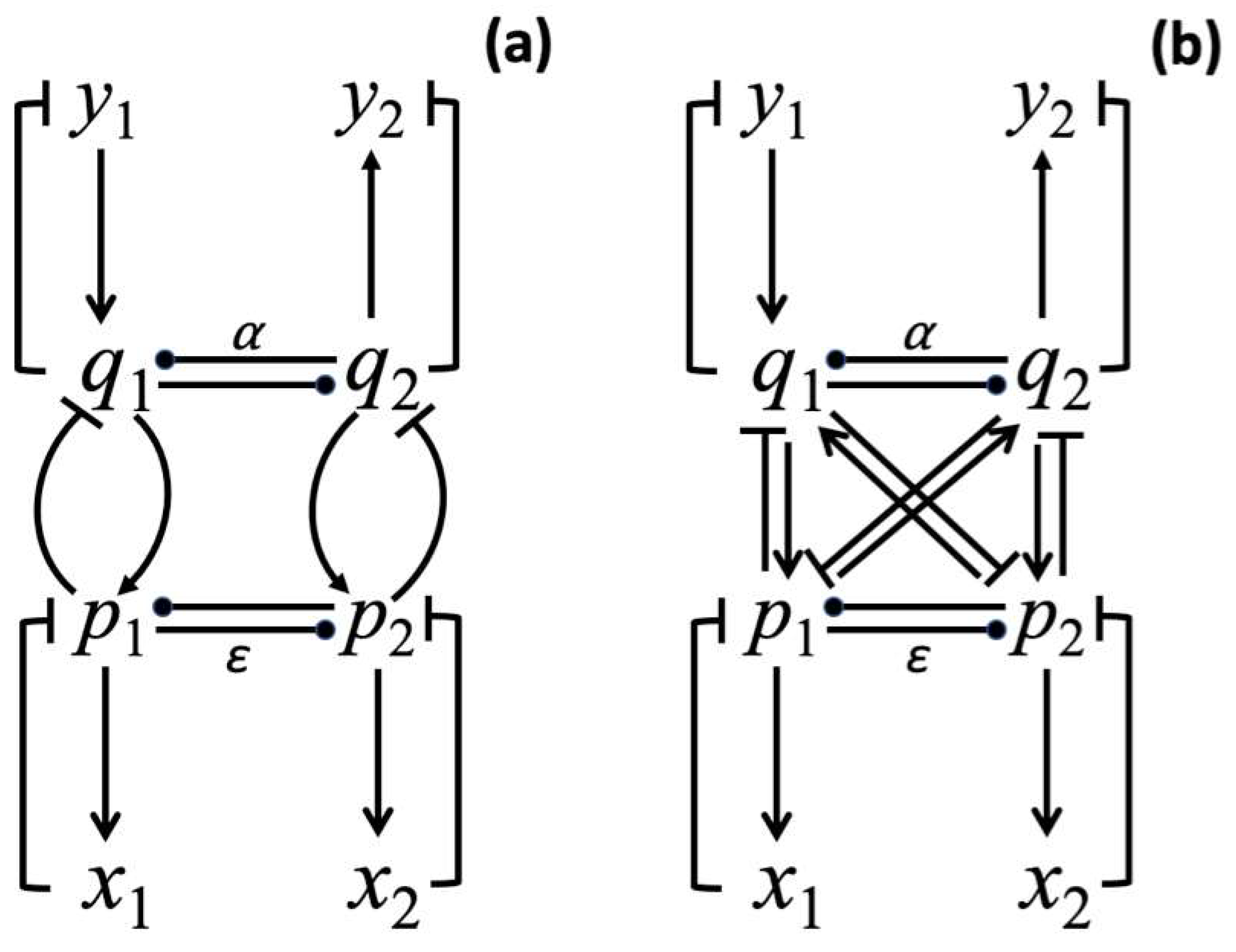
where $\epsilon$ and $\alpha$ are parameters describing the mutual interactions between p-processes and between q-processes correspondingly, see Figure 1a,b. The $f_1\left(q_1,q_2\right)$, $f_1\left(q_1,q_2\right)$ and $g_1\left(p_1,p_2\right)$, $g_1\left(p_1,p_2\right)$ functions describe the binding between the $\overrightarrow{P}$ and $\overrightarrow{Q}$ sets of processes. Generally, a function that depends on a difference between oscillating variables can be used to achieve a synchronization of two oscillators [44] (pp. 123–136). Two oscillators that communicate the phase to one another can be drawn into synchrony over time. In System (1), I assume that the interaction among processes is realized via negative feedback loops (see Figure 1a,b that show two possible coupling mechanisms between the $\overrightarrow{P}$ and $\overrightarrow{Q}$ sets of processes). Mathematically, I consider the following two interaction schemes: (a) $f_1\left(q_1,q_2\right)=q_1$, $f_2\left(q_1,q_2\right)=q_2$, $g_1\left(p_1,p_2\right)=-p_1$, $g_2\left(p_1,p_2\right)=-p_2$, where this formulation corresponds to the mechanism shown in Figure 1a,b $f_1\left(q_1,q_2\right)=q_1-q_2$, $f_2\left(q_1,q_2\right)=q_2-q_1$, $g_1\left(p_1,p_2\right)=p_2-p_1$, $g_2\left(p_1,p_2\right)=p_1-p_2$ is according to the mechanism shown in Figure 1b.

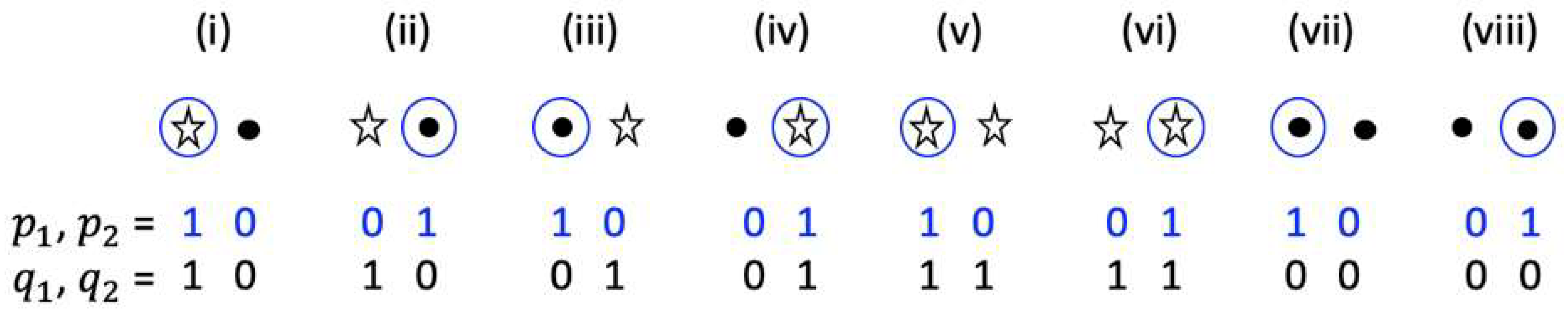
I assume that the $\overrightarrow{P}$ and $\overrightarrow{Q}$ processes occur in response to two different percepts. For example, the state of ($p_1$, $p_2$) can represent the processes in response to the specific position selected by attention, which is indicated by a blue circle in Figure 2, and the state of ($q_1$, $q_2$) can represent the processes in response to the presence or absence of a light stimulus at the selected location (shown by a star sign or black dot in Figure 2). Hence, I distinguish the position of a spot that can be either dark or bright by focusing our attention either on the bright spot (e.g., case (i) in Figure 2) or on the dark spot (e.g., case (ii) in Figure 2). Therefore, my model represents perceptual binding occurring for two percepts that include the position in space and an attribute that is assigned to each position. The position selection is represented by the $p_1$ and $p_2$ processes. The initial value for the $p_1$ or $p_2$ variable is set to 1 if the corresponding position is selected or to zero otherwise (see Figure 2). Similarly, the initial value for the process $q_1$ or $q_2$ is set to 1 if a light stimulus is present, otherwise the initial value for $q_1$ or $q_2$ is set to zero. All corresponding initial values for $p_1$, $p_2$, $q_1$, $q_2$ processes for cases (i)–(viii) are shown in Figure 2. Simulation results of these cases are provided in the Results section of this manuscript.

System (1) consists of a system of linear differential equations that has a solution that can be, in principle, expressed in algebraic form. However, eight eigenvalues and eigenvectors cannot be written in a concise form to fit into this text and be easily analyzed. Therefore, here, I present numerical solutions obtained for different initial conditions and parameter values that produce distinct numerical results. XPP/XPPAUT software (http://www.math.pitt.edu/~bard/xpp/xpp.html, accessed on 12 January 2022) was used to solve System (1) and compute two-parameter bifurcation diagrams. XPP codes that were used to produce all results presented in this work are provided in Appendix A. since System (1) is linear, I do not perform a global sensitivity analysis that is a common tool to analyze nonlinear systems to determine the variations in the model outputs depending on the variations in inputs [45,46]. Nevertheless, the dynamic behavior of System (1) has been already shown to be robust against the noise [42].

3. Results

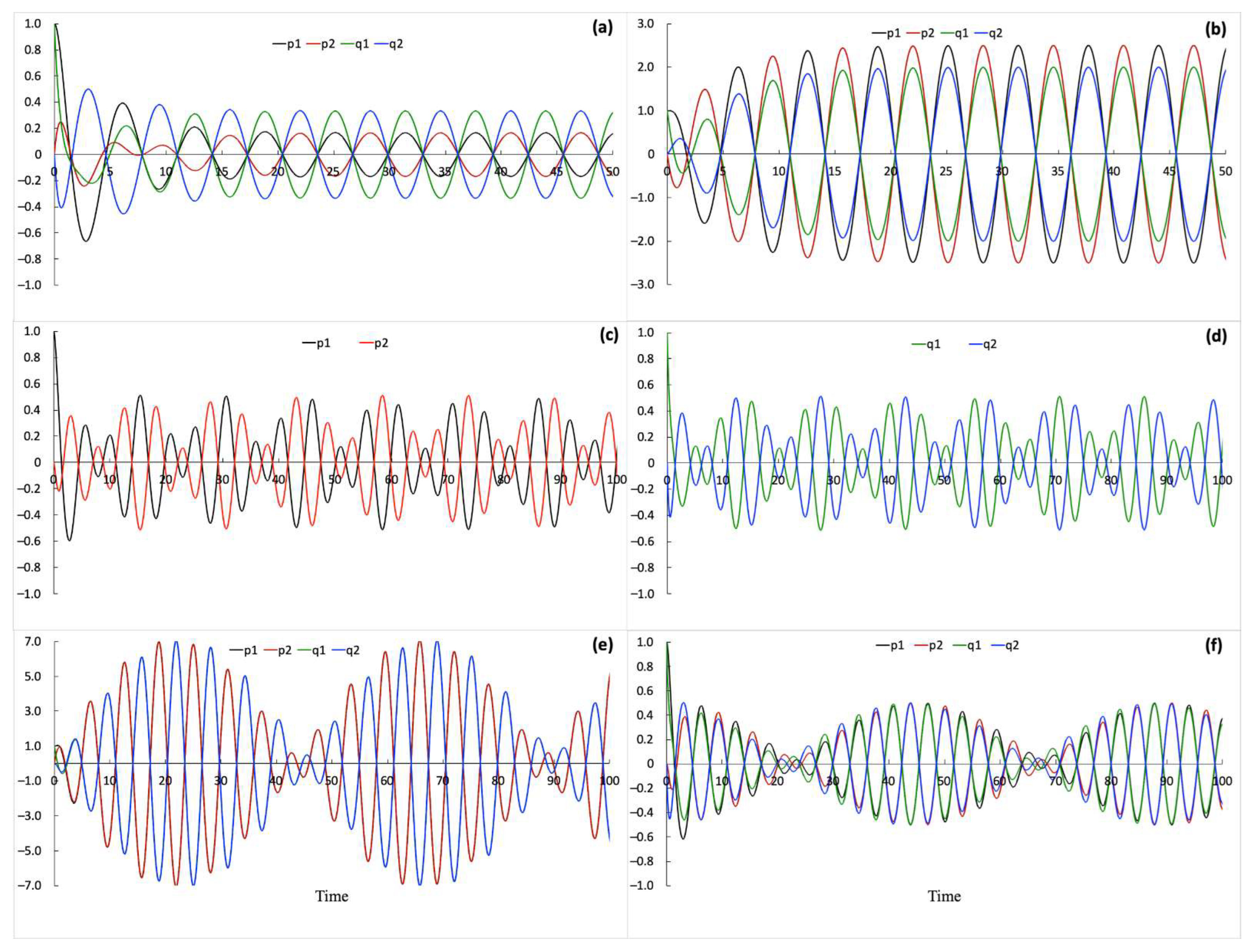
First, I analyze System (1) by considering the interaction scheme shown in Figure 1a. I explore solutions of System (1) for different values of $\epsilon$ and $\alpha$ parameters to identify distinct dynamic regimes that the system of coupled processes can exhibit. Thus, $\epsilon$ and $\alpha$ serve as bifurcation parameters of the system. As shown in Figure 3, the dynamic behavior of the $\overrightarrow{P}$ and $\overrightarrow{Q}$ processes depends on $\epsilon$ and $\alpha$ parameter values. The feedback loops connecting the two sets of processes induce a complex mutual modulation among the interacting processes. Consequently, variations in amplitude, frequency, and temporal relationships among processes depending on parameter values are observed. Similar amplitude modulation or distortion is commonly observed for two coupled oscillators when the coupling is not strong enough to bring the phases of two oscillators into synchrony over time [44] (pp. 123–136). Closely, the strong amplitude modulation in System (1) occurs when one parameter, either $\epsilon$ or $\alpha$, is much smaller than the other (see Figure 3e,f). Therefore, amplitude distortion is likely to be observed in a system that is composed of two interacting subsystems such that one subsystem is described by weak internal coupling parameters and the other is described by strong internal coupling parameters. Interestingly, I also observe small amplitude variations when both $\epsilon$ and $\alpha$ have values close to −1. These variations also occur due to interactions between the $\overrightarrow{P}$ and $\overrightarrow{Q}$ processes. When the $\overrightarrow{P}$ and $\overrightarrow{Q}$ processes are decoupled, the amplitude variations disappear. Thus, the amplitude distortion in experimentally recorded signals could indicate binding.

Here, I only present periodic solutions with sustained oscillations; however, the system also exhibits damped oscillations and unstable sources or oscillations with growing amplitude as well. The periodic solutions of System (1) with sustained oscillations are found for the following ranges of parameters:

$$\begin{gathered} \alpha =-\frac{\epsilon +2}{\epsilon +1} \mathrm{for} -2<\epsilon \le -\sqrt{2} \mathrm{and} 0<\epsilon \le \sqrt{2} \\ \alpha =\frac{\epsilon -2}{\epsilon -1} \mathrm{for} -\sqrt{2}\le \epsilon <0 \mathrm{and} \sqrt{2}\le \epsilon <2 \\ \alpha =-\epsilon -2 \mathrm{for} -2<\epsilon <0 \\ \alpha =-\epsilon +2 \mathrm{for} 0<\epsilon <2. \end{gathered}$$

(2)

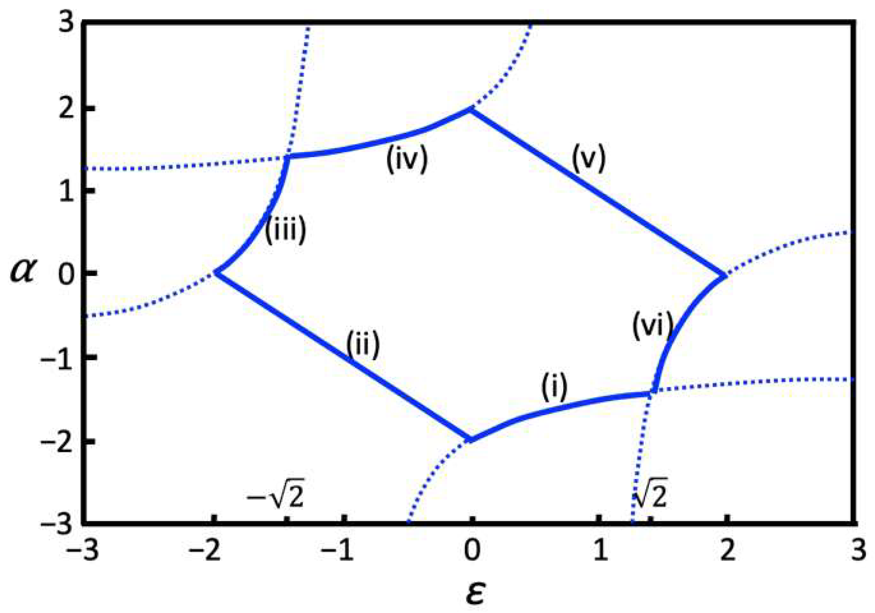
The corresponding two-parameter bifurcation diagram is shown in Figure 4. The diagram is obtained numerically as explained in the Methods section and agrees with the analytical solutions described by the System of Equation (2). The parameter ranges marked as (i) and (iii) in Figure 4 correspond to the first equation in System (2); the regions marked as (iv) and (vi) in Figure 4 correspond to the second equation in System (2); the line marked as (ii) in Figure 4 corresponds to the third equation in System (2) and the line labeled with (v) in Figure 4 corresponds to the last equation in System (2). Oscillations are observed with varying amplitudes for parameter values along the (ii) and (v) lines shown in Figure 4. Figure 3c,d,f provide examples of oscillations obtained using parameter values from region (ii) and Figure 3e shows simulations obtained using parameter values from region (v). Oscillations produced using parameter values from regions (i) and (iii) are shown in Figure 3a and Figure 3b, respectively. Oscillations for parameter values taken in regions (iv) and (vi) have constant amplitude similar to those shown in Figure 3a,b but $p_1$ and $q_1$ oscillate in phase with $p_2$ and $q_2,$ respectively (not shown). Overall, System (1) combined with the interaction scheme shown in Figure 1a produces a diverse repertoire of periodic solutions with sustained oscillations that depend on the system’s parameters.

Next, I fix the ε and α parameter values and investigate the solutions of System (1) depending on the different initial conditions that are shown in Figure 2. ε and α parameter values are taken from region (ii), shown in Figure 4, which are also described by the third equation in System (2). For these parameter values, the system of processes exhibits sustained oscillations for both interaction schemes shown in Figure 1a,b. Thus, we can compare how different interaction schemes perform in solving a discrimination task by differentiating inputs shown in Figure 2.

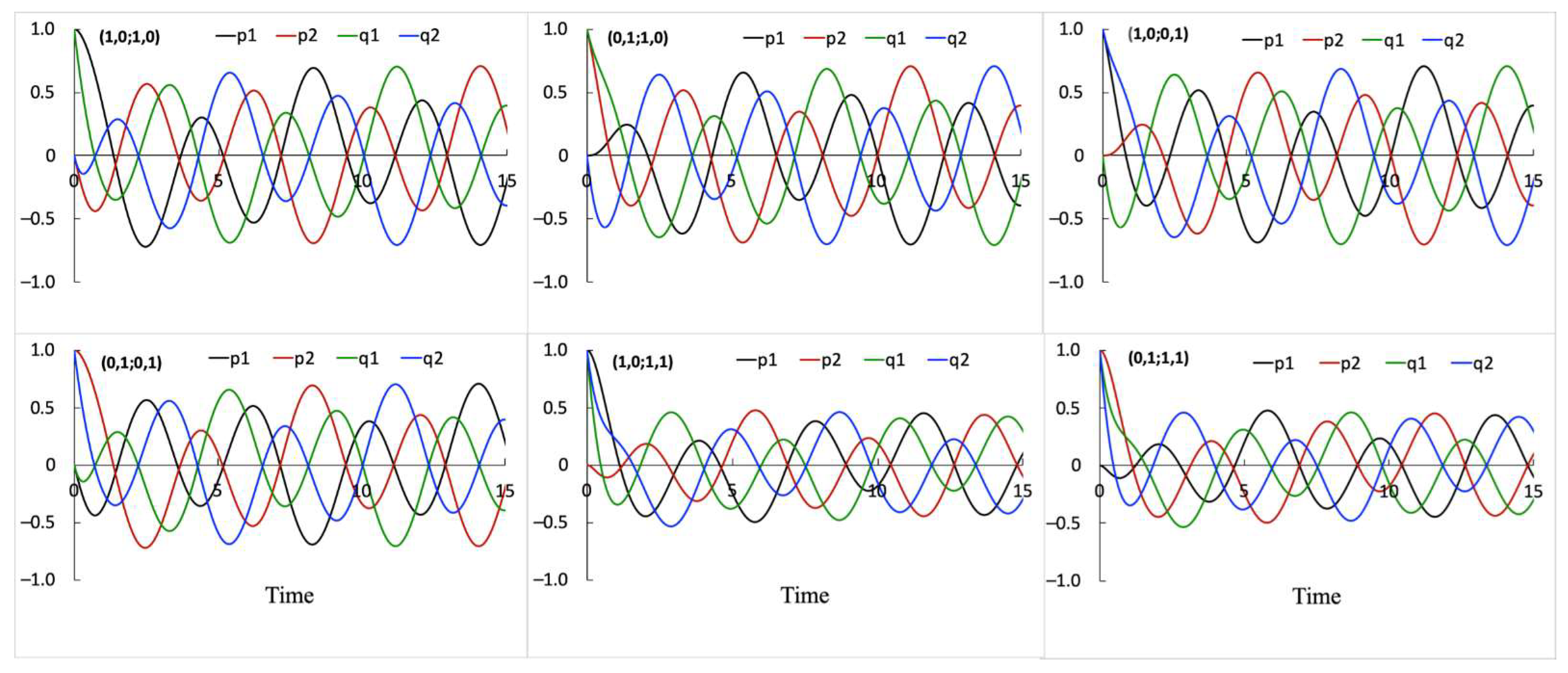
Six conditions (i)–(vi) shown in Figure 2 produce distinct dynamic relationships among $p_1$, $p_2$, $q_1$, $q_2$ processes (see Figure 5). However, two conditions (vii) and (viii), shown in Figure 2, produce the same dynamic relationships among processes as obtained for the (v) and (vi) conditions, respectively. Therefore, the system can discriminate (i)–(vi) initial inputs but cannot discriminate (vii) and (viii) from (v) and (vi) inputs. The latter means that the position in space that is homogeneously bright is identical to the same position in space that is homogeneously dark. Perhaps, these inputs can be discriminated if more complex interactions representing binding or a system with more states and hierarchical levels of binding interactions between these states are used.

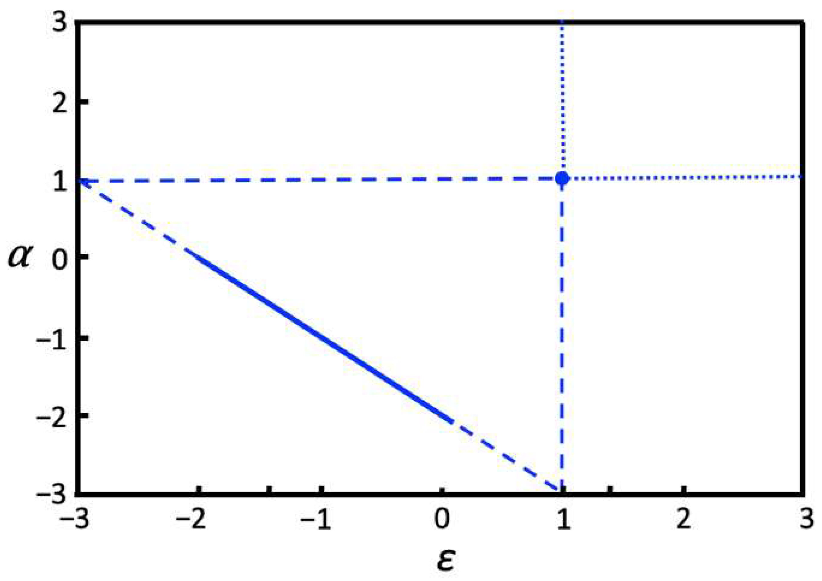
Solving and analyzing System (1) for the second interaction scheme shown in Figure 1b, I also identified ε and α parameter values for which the periodic solutions with sustained oscillations are obtained. A two-parameter bifurcation diagram that summarizes parameter ranges with periodic solutions is shown in Figure 6. Oscillations for parameter values along the solid line in Figure 6 are qualitatively similar to those that are shown in Figure 5 and obtained for the same range of parameters: α = − ε − 2 for −2 < ε < 0, however, the frequency of oscillations is higher (see Figure S1 in the Supplementary Materials). Also, System (1) combined with the interaction scheme in Figure 1b performs equally well to that of the scheme shown in Figure 1a on the task to discriminate different inputs that are shown in Figure 2. However, comparing two-parameter bifurcation diagrams in Figure 4 and Figure 6, the diagram in Figure 4 shows significantly more parameter ranges where the system exhibits sustained oscillations. Therefore, despite the fact that the interaction scheme in Figure 1b has more interactions than the interaction scheme shown in Figure 1a, the latter, simpler interaction scheme produces a more diverse dynamic behavior of the system. Thus, the more comprehensive interaction network that integrates information from many network nodes does not necessarily result in a more diverse dynamic repertoire.

4. Discussion

Mechanistic modeling has become a very popular tool that allows one to not simply describe the system components but to also analyze, understand, and explain the dynamic behavior of the system. This mechanistic approach has been successfully applied to modelling nerve action potential [47], neurodynamics in the olfactory system [48], dynamics of ecological networks [49], molecular signaling pathways [50], and complex molecular mechanisms determining cell fate [44,51,52,53,54]. However, building mechanistic models of consciousness is undoubtedly one of the most challenging tasks. By using my previous dynamic modeling framework to describe a percept [41,42,43], here, I developed a dynamic mechanistic model of perceptual binding.

The perceptual binding concept is compatible with the Integrated Information and Temporo-Spatial theories of consciousness as well as with some classical neural network models [2,25,29,30,31,32]. However, as put forward by von der Malsburg, for example, the classical neural network models interpret a brain state as a static vector ignoring the fact that recorded neural signals are not constant over any fixed time scale [2]. By contrast, in my model, the states are encoded in the dynamical processes that continuously alternate, yet their specific relationships that encode information are maintained over time. This continuous realization of specific relationships among processes in the system is an important concept in my modeling framework. The main assumption of my approach is that consciousness is a dynamical process, not a capacity, memory, or information, as elaborated by James, 1904 [55].

My dynamic approach is comparable to Freeman’s framework developed to describe population neurodynamics in the olfactory system [48]. His system of ordinary differential equations constructed in conformance with the anatomical and physiological properties of the olfactory system has been successful in explaining electrophysiological recordings of impulse responses. Different oscillations have been observed including complex and highly dimensional oscillations with varying amplitudes and a pattern that repeats itself (see Figure 6 on page 301 in Ref. [48]). While my simulation results may not be directly comparable with the dynamic behavior of neuronal systems or with electroencephalographic brain recordings, my model provides a qualitative representation of how binding can influence and change neural oscillations. Although, I analyzed a simple system in which the space is represented by two points described by the ($p_1,p_2$) processes and each point was characterized only by two states ($q_1,q_2$), the system can be scaled to n-points each with m-states (n, m > 2) as shown in Kraikivski, 2020, 2021 [41,42]. However, the application of sets with many states to investigate binding would only complicate the analysis and interpretation of results.

I analyzed a system of two sets of processes representing two different percepts and found that the system exhibits different dynamic behavior depending on initial conditions (see Figure 5) and is capable of distinguishing different combinations of initial inputs shown in Figure 2. Therefore, my approach can be an alternative to classical neural networks that fail to solve a discrimination task in Frank Rosenblatt’s example with four neurons where two neurons learn to recognize the object shape and the other two indicate the position of objects [2,56]. The output reads of such a four-neuron classical network include two shapes (e.g., square, triangle) and two positions (left, right), however, whether a specific shape is on the left side or on the right side remains indistinguishable.

I investigated two interaction schemes (see Figure 1a,b) describing binding between the sets of processes. For both wiring schemes, different dynamic oscillatory regimes were identified. Remarkably, despite the comprehensive level of interactions among processes and, therefore, a higher level of information integration, the interaction scheme shown in Figure 1b does not result in overly complex dynamic behavior, as opposed to the interaction scheme in Figure 1a, which produces a more diverse repertoire of oscillating regimes (see Figure 3, Figure 4 and Figure 6). This result appears to be opposite to what would be expected in Integrated Information Theory, which identifies consciousness with the ability of the system to integrate information.

In conclusion, my mechanistic model can help one gain a better understanding of how binding can affect the dynamic behavior of the systems that involve perceptual binding. Although, the real neural oscillatory signals differ from oscillations shown in Figure 3 and Figure 5, the qualitative conclusions derived in this work can be applied to understand the dynamic outcomes recorded in real neural systems. For example, my results suggest that amplitude modulation or distortion detected in experimentally recorded signals can be used to detect binding and reveal some properties of interacting subsystems. Furthermore, binding cannot be merely the result of synchronization of signals or temporal correlation that can spontaneously occur or be set in two non-interacting systems. Binding may only occur when processes interact, resulting in modulation and superposition of signals. Some approach limitations and the discussion of how the results can be compared to electroencephalograms (EEG) and functional magnetic resonance imaging (fMRI) recordings has been discussed in Kraikivski, 2020 [41].

References

- Roskies, A.L. The binding problem. Neuron 1999, 24, 7–9. [Google Scholar] [CrossRef] [Green Version]
- Von der Malsburg, C. The what and why of binding: The modeler’s perspective. Neuron 1999, 24, 95–104. [Google Scholar] [CrossRef] [Green Version]
- Goodale, M.A.; Milner, A.D.; Jakobson, L.S.; Carey, D.P. A neurological dissociation between perceiving objects and grasping them. Nature 1991, 349, 154–156. [Google Scholar] [CrossRef] [PubMed]
- Goodale, M.A.; Meenan, J.P.; Bulthoff, H.H.; Nicolle, D.A.; Murphy, K.J.; Racicot, C.I. Separate neural pathways for the visual analysis of object shape in perception and prehension. Curr. Biol. 1994, 4, 604–610. [Google Scholar] [CrossRef]
- Bogen, J.E.; Fisher, E.D.; Vogel, P.J. Cerebral commissurotomy. A second case report. JAMA 1965, 194, 1328–1329. [Google Scholar] [CrossRef]
- De Haan, E.H.F.; Corballis, P.M.; Hillyard, S.A.; Marzi, C.A.; Seth, A.; Lamme, V.A.F.; Volz, L.; Fabri, M.; Schechter, E.; Bayne, T.; et al. Split-Brain: What We Know Now and Why This is Important for Understanding Consciousness. Neuropsychol. Rev. 2020, 30, 224–233. [Google Scholar] [CrossRef]
- Wolfe, J.M.; Cave, K.R. The psychophysical evidence for a binding problem in human vision. Neuron 1999, 24, 11–17. [Google Scholar] [CrossRef] [Green Version]
- Treisman, A. Solutions to the binding problem: Progress through controversy and convergence. Neuron 1999, 24, 105–110. [Google Scholar] [CrossRef] [Green Version]
- Altieri, N.; Stevenson, R.A.; Wallace, M.T.; Wenger, M.J. Learning to associate auditory and visual stimuli: Behavioral and neural mechanisms. Brain Topogr. 2015, 28, 479–493. [Google Scholar] [CrossRef] [Green Version]
- Stevenson, R.A.; Zemtsov, R.K.; Wallace, M.T. Individual differences in the multisensory temporal binding window predict susceptibility to audiovisual illusions. J. Exp. Psychol. Hum. Percept. Perform. 2012, 38, 1517–1529. [Google Scholar] [CrossRef] [Green Version]
- Colonius, H.; Diederich, A. Multisensory interaction in saccadic reaction time: A time-window-of-integration model. J. Cogn. Neurosci. 2004, 16, 1000–1009. [Google Scholar] [CrossRef] [PubMed]
- Diederich, A.; Colonius, H. Crossmodal interaction in speeded responses: Time window of integration model. In Progress in Brain Research; Raab, M., Johnson, J.G., Heekeren, H.R., Eds.; Elsevier: Amsterdam, The Netherlands, 2009; Volume 174, pp. 119–135. [Google Scholar]
- Horváth, J.; Czigler, I.; Winkler, I.; Teder-Sälejärvi, W.A. The temporal window of integration in elderly and young adults. Neurobiol. Aging 2007, 28, 964–975. [Google Scholar] [CrossRef] [PubMed]
- Diederich, A.; Colonius, H.; Schomburg, A. Assessing age-related multisensory enhancement with the time-window-of-integration model. Neuropsychologia 2008, 46, 2556–2562. [Google Scholar] [CrossRef] [PubMed]
- Baum, S.H.; Stevenson, R. Shifts in Audiovisual Processing in Healthy Aging. Curr. Behav. Neurosci. Rep. 2017, 4, 198–208. [Google Scholar] [CrossRef]
- Hillock, A.R.; Powers, A.R.; Wallace, M.T. Binding of sights and sounds: Age-related changes in multisensory temporal processing. Neuropsychologia 2011, 49, 461–467. [Google Scholar] [CrossRef] [Green Version]
- Shams, L.; Kamitani, Y.; Shimojo, S. Visual illusion induced by sound. Cogn. Brain Res. 2002, 14, 147–152. [Google Scholar] [CrossRef]
- Shams, L.; Kamitani, Y.; Shimojo, S. What you see is what you hear. Nature 2000, 408, 788. [Google Scholar] [CrossRef]
- Sekuler, R.; Sekuler, A.B.; Lau, R. Sound alters visual motion perception. Nature 1997, 385, 308. [Google Scholar] [CrossRef]
- Bayne, T.; Oxford University Press. The Unity of Consciousness; Oxford University Press: Oxford, UK, 2010. [Google Scholar]
- Revonsuo, A. Binding and the Phenomenal Unity of Consciousness. Conscious. Cogn. 1999, 8, 173–185. [Google Scholar] [CrossRef] [Green Version]
- Damasio, A.R. Time-locked multiregional retroactivation: A systems-level proposal for the neural substrates of recall and recognition. Cognition 1989, 33, 25–62. [Google Scholar] [CrossRef]
- Gray, C.M. The temporal correlation hypothesis of visual feature integration: Still alive and well. Neuron 1999, 24, 31–47. [Google Scholar] [CrossRef] [Green Version]
- Singer, W. Neuronal synchrony: A versatile code for the definition of relations? Neuron 1999, 24, 49–65. [Google Scholar] [CrossRef] [Green Version]
- Von der Malsburg, C. Binding in models of perception and brain function. Curr. Opin. Neurobiol. 1995, 5, 520–526. [Google Scholar] [CrossRef] [Green Version]
- Fingelkurts, A.A.; Fingelkurts, A.A.; Neves, C.F.H. Phenomenological architecture of a mind and Operational Architectonics of the brain: The unified metastable continuum. J. New Math. Nat. Comput. 2009, 5, 221–244. [Google Scholar] [CrossRef] [Green Version]
- Fingelkurts, A.A.; Fingelkurts, A.A. Mind as a nested operational architectonics of the brain. Phys. Life Rev. 2012, 9, 49–50. [Google Scholar] [CrossRef]
- Fingelkurts, A.A.; Fingelkurts, A.A.; Neves, C.F.H. Consciousness as a phenomenon in the operational architectonics of brain organization: Criticality and self-organization considerations. Chaos Solitons Fractals 2013, 55, 13–31. [Google Scholar] [CrossRef]
- Northoff, G. What the brain’s intrinsic activity can tell us about consciousness? A tri-dimensional view. Neurosci. Biobehav. Rev. 2013, 37, 726–738. [Google Scholar] [CrossRef]
- Northoff, G.; Huang, Z.R. How do the brain’s time and space mediate consciousness and its different dimensions? Temporo-spatial theory of consciousness (TTC). Neurosci. Biobehav. Rev. 2017, 80, 630–645. [Google Scholar] [CrossRef]
- Seth, A.K.; Izhikevich, E.; Reeke, G.N.; Edelman, G.M. Theories and measures of consciousness: An extended framework. Proc. Natl. Acad. Sci. USA 2006, 103, 10799–10804. [Google Scholar] [CrossRef] [Green Version]
- Tononi, G.; Edelman, G.M. Consciousness and complexity. Science 1998, 282, 1846–1851. [Google Scholar] [CrossRef]
- Dehaene, S.; Changeux, J.P. Experimental and theoretical approaches to conscious processing. Neuron 2011, 70, 200–227. [Google Scholar] [CrossRef] [PubMed] [Green Version]
- Dehaene, S.; Charles, L.; King, J.R.; Marti, S. Toward a computational theory of conscious processing. Curr. Opin. Neurobiol. 2014, 25, 76–84. [Google Scholar] [CrossRef] [PubMed] [Green Version]
- Tononi, G. An information integration theory of consciousness. BMC Neurosci. 2004, 5, 42. [Google Scholar] [CrossRef] [PubMed] [Green Version]
- Tononi, G. Consciousness as Integrated Information: A Provisional Manifesto. Biol. Bull. 2008, 215, 216–242. [Google Scholar] [CrossRef] [PubMed]
- Tononi, G. Information integration: Its relevance to brain function and consciousness. Arch. Ital. Biol. 2010, 148, 299–322. [Google Scholar] [PubMed]
- Shadlen, M.N.; Movshon, J.A. Synchrony unbound: A critical evaluation of the temporal binding hypothesis. Neuron 1999, 24, 67–77. [Google Scholar] [CrossRef] [PubMed] [Green Version]
- Riesenhuber, M.; Poggio, T. Are cortical models really bound by the “binding problem”? Neuron 1999, 24, 87–93. [Google Scholar] [CrossRef] [Green Version]
- Ghose, G.M.; Maunsell, J. Specialized representations in visual cortex: A role for binding? Neuron 1999, 24, 79–85. [Google Scholar] [CrossRef] [Green Version]
- Kraikivski, P. Systems of Oscillators Designed for a Specific Conscious Percept. New Math. Nat. Comput. 2020, 16, 73–88. [Google Scholar] [CrossRef] [Green Version]
- Kraikivski, P. Implications of Noise on Neural Correlates of Consciousness: A Computational Analysis of Stochastic Systems of Mutually Connected Processes. Entropy 2021, 23, 583. [Google Scholar] [CrossRef]
- Kraikivski, P. Building Systems Capable of Consciousness. Mind Matter 2017, 15, 185–195. [Google Scholar]
- Kraikivski, P. (Ed.) Case Studies in Systems Biology, 1st ed.; Springer: Cham, Switzerland, 2021; p. 310. [Google Scholar] [CrossRef]
- Pianosi, F.; Beven, K.; Freer, J.; Hall, J.W.; Rougier, J.; Stephenson, D.B.; Wagener, T. Sensitivity analysis of environmental models: A systematic review with practical workflow. Environ. Model. Softw. 2016, 79, 214–232. [Google Scholar] [CrossRef]
- Li, J.; Convertino, M. Optimal Microbiome Networks: Macroecology and Criticality. Entropy 2019, 21, 506. [Google Scholar] [CrossRef] [PubMed] [Green Version]
- Hodgkin, A.L.; Huxley, A.F. A quantitative description of membrane current and its application to conduction and excitation in nerve. J. Physiol. 1952, 117, 500–544. [Google Scholar] [CrossRef] [PubMed]
- Freeman, W.J.; SpringerLink (Online service). Neurodynamics: An Exploration in Mesoscopic Brain Dynamics. In Perspectives in Neural Computing; Springer: London, UK, 2000. [Google Scholar]
- Loeuille, N.; Loreau, M. Evolutionary emergence of size-structured food webs. Proc. Natl. Acad. Sci. USA 2005, 102, 5761–5766. [Google Scholar] [CrossRef] [PubMed] [Green Version]
- Jalihal, A.P.; Kraikivski, P.; Murali, T.M.; Tyson, J.J. Modeling and analysis of the macronutrient signaling network in budding yeast. Mol. Biol. Cell. 2021, 32, ar20. [Google Scholar] [CrossRef]
- Kraikivski, P.; Chen, K.C.; Laomettachit, T.; Murali, T.M.; Tyson, J.J. From START to FINISH: Computational analysis of cell cycle control in budding yeast. NPJ Syst. Biol. Appl. 2015, 1, 15016. [Google Scholar] [CrossRef] [Green Version]
- Tyson, J.J.; Laomettachit, T.; Kraikivski, P. Modeling the dynamic behavior of biochemical regulatory networks. J. Theor. Biol. 2019, 462, 514–527. [Google Scholar] [CrossRef]
- Tyson, J.J.; Novak, B. A Dynamical Paradigm for Molecular Cell Biology. Trends Cell. Biol. 2020, 30, 504–515. [Google Scholar] [CrossRef]
- Jung, Y.; Kraikivski, P.; Shafiekhani, S.; Terhune, S.S.; Dash, R.K. Crosstalk between Plk1, p53, cell cycle, and G2/M DNA damage checkpoint regulation in cancer: Computational modeling and analysis. NPJ Syst. Biol. Appl. 2021, 7, 46. [Google Scholar] [CrossRef]
- James, W. Does ‘Consciousness’ Exist? J. Philos. Psychol. Sci. Methods 1904, 1, 477–491. [Google Scholar] [CrossRef]
- Rosenblatt, F. Principles of Neurodynamics; Perceptrons and the Theory of Brain Mechanisms; Spartan Books: Washington, DC, USA, 1962. [Google Scholar]
Figure 1.
Two different influence schemes for processes described by the system of Equation (1). (a) Binding between and sets of processes is gained through interaction of with and with processes. In neural systems such specific winning links can be established via training in response to different combinations of input stimuli. Here, negative feedback loops are used to realize connections between and as well as between and . (b) Binding between and sets of processes in which all , , , processes are mutually interconnected via negative feedback loops. Arrow-headed lines represent a positive influence and bar-headed lines represent a negative influence. The dot-headed lines represent positive or negative influence depending on the sign of the α and ε parameters.
Figure 2.
Seven different combinations of two distinct types of inputs representing percepts and the corresponding initial values of (, ) and (, ) processes. Each combination consists of two possible positions and the presence/absence of a light stimulus at these positions. The presence of a light stimulus at a position is indicated by the star sign and the absence of light is indicated by the black dot. A specific position is assumed to be selected by attention, which is indicated by the blue circle. For example, for case (i), the focus is on the bright spot, while for case (ii), the focus is on the dark spot.
Figure 3.
Oscillatory behavior observed in the dynamic system of coupled processes. Oscillations of (, ) and (, ) processes are obtained using the following parameter values: (a) ε = 1, α = −1.5; (b) ε = −1.8, α = 0.25; (c,d) ε = −0.1, α = −1.9, where the (, ) and (, ) processes are shown on separate figure panels for better visualization; (e) ε = 1.99, α = 0.01, note that shortly after the starting values the (, ) and (, ) processes begin and continue to overlap over time; (f) ε = −0.01, α = −1.99. All simulations are obtained using the same initial conditions: (, , , ) = (1, 0, 1, 0) that corresponds to case (i) in Figure 2, and (, , , ) = (0, 0, 0, 0).
Figure 4.
Two-parameter bifurcation diagram for the interaction scheme shown in Figure 1a. Oscillations occur for ε and α parameter values along solid curves marked as (i)–(v). To demonstrate agreement between numerical and analytical solutions, the dotted curves are drawn by plotting the following functions: α = −(ε + 2)/(ε + 1) and α = (ε − 2)/(ε − 1), which overlap with solid curves (iii), (i) and (iv), (vi) obtained numerically in corresponding regions.
Figure 5.
The change in dynamic relationships among , , , processes depend on initial conditions. Six initial conditions (i)–(vi) shown in Figure 2 are used to produce these simulation results. These conditions induce distinct dynamic relationships among processes and, thereby, can be discriminated by the system. The initial conditions are indicated in the figures as two pairs of digits corresponding to initial values of (, ; , ) shown in parenthesis at the upper left corner of each figure panel. All simulations are obtained using the interaction scheme shown in Figure 1a and the following parameter values: ε = −1, α = −1.
Figure 6.
Two-parameter bifurcation diagram for the interaction scheme shown in Figure 1b. The solid line, α = − ε − 2 for −2 < ε < 0, shows the parameter values where both and oscillate and the relationships between and and and are maintained over time. For these parameter values, and oscillate out of phase and with varying amplitudes. Dashed lines show the parameter values where oscillations exist but either the relationships between p-processes or q-processes are no longer maintained (diagonal dashed lines), or only one set of processes oscillate while another set of processes does not exhibit oscillatory dynamics (vertical and horizontal dashed lines). Dotted lines show parameter ranges where oscillations exist only if either or starts with zero initial conditions and, thus, only p-processes or q-processes oscillate, which is equivalent to the situation when and are decoupled and independent. At the point (α = 1, ε = 1), both p-processes and q-processes oscillate in phase with constant amplitudes.
Publisher’s Note: MDPI stays neutral with regard to jurisdictional claims in published maps and institutional affiliations. |
© 2022 by the author. Licensee MDPI, Basel, Switzerland. This article is an open access article distributed under the terms and conditions of the Creative Commons Attribution (CC BY) license (https://creativecommons.org/licenses/by/4.0/).
Share and Cite
MDPI and ACS Style
Kraikivski, P. A Dynamic Mechanistic Model of Perceptual Binding. Mathematics 2022, 10, 1135. https://doi.org/10.3390/math10071135
AMA Style
Kraikivski P. A Dynamic Mechanistic Model of Perceptual Binding. Mathematics. 2022; 10(7):1135. https://doi.org/10.3390/math10071135
Chicago/Turabian StyleKraikivski, Pavel. 2022. "A Dynamic Mechanistic Model of Perceptual Binding" Mathematics 10, no. 7: 1135. https://doi.org/10.3390/math10071135
Note that from the first issue of 2016, this journal uses article numbers instead of page numbers. See further details here.