Proving Feasibility of a Docking Mission: A Contractor Programming Approach

Abstract

Recent advances in computational power, algorithms, and sensors allow robots to perform complex and dangerous tasks, such as autonomous missions in space or underwater. Given the high operational costs, simulations are run beforehand to predict the possible outcomes of a mission. However, this approach is limited as it is based on parameter space discretization and therefore cannot be considered a proof of feasibility. To overcome this limitation, set-membership methods based on interval analysis, guaranteed integration, and contractor programming have proven their efficiency. Guaranteed integration algorithms can predict the possible trajectories of a system initialized in a given set in the form of tubes of trajectories. The contractor programming consists in removing the trajectories violating predefined constraints from a system’s tube of possible trajectories. Our contribution consists in merging both approaches to allow for the usage of differential constraints in a contractor programming framework. We illustrate our method through examples related to robotics. We also released an open-source implementation of our algorithm in a unified library for tubes, allowing one to combine it with other constraints and increase the number of possible applications.

1. Introduction

1.1. Context

Robots are usually designed to replace humans in difficult, dangerous, or repetitive jobs. Their application domains range from underwater inspection and maintenance to space exploration, assembly lines, search and rescue missions, and military applications. The number of missions that robots can tackle is ever increasing, thanks to advances in computational power, algorithms, and sensors that allow the robots to better understand their environment and act on it.

Therefore, the robots become more autonomous and can achieve most of the tasks of a mission without human supervision. However, some specific tasks remain challenging, and their failure could cause equipment damage, loss, and human casualties. Consider, for example, a rendezvous task. The latter is a component of different types of missions: recovering an autonomous underwater vehicle using a docking station (see Figure 1a and [1,2,3]), docking a spacecraft onto another one (Figure 1b), or destroying a rocket using a missile. While algorithms and sensors exist to perform localization, control, and navigation tasks, they usually do not ensure the feasibility and success of the mission. This proof is essential since failure involves unpredictable costs or casualties. Therefore, there exists a need for methods that allow for the proving of the feasibility of autonomous missions, i.e., that would allow the operators to be sure that a robot, equipped with a specific range of sensors and algorithms and deployed in a particular area, would be able to reach another specific one. 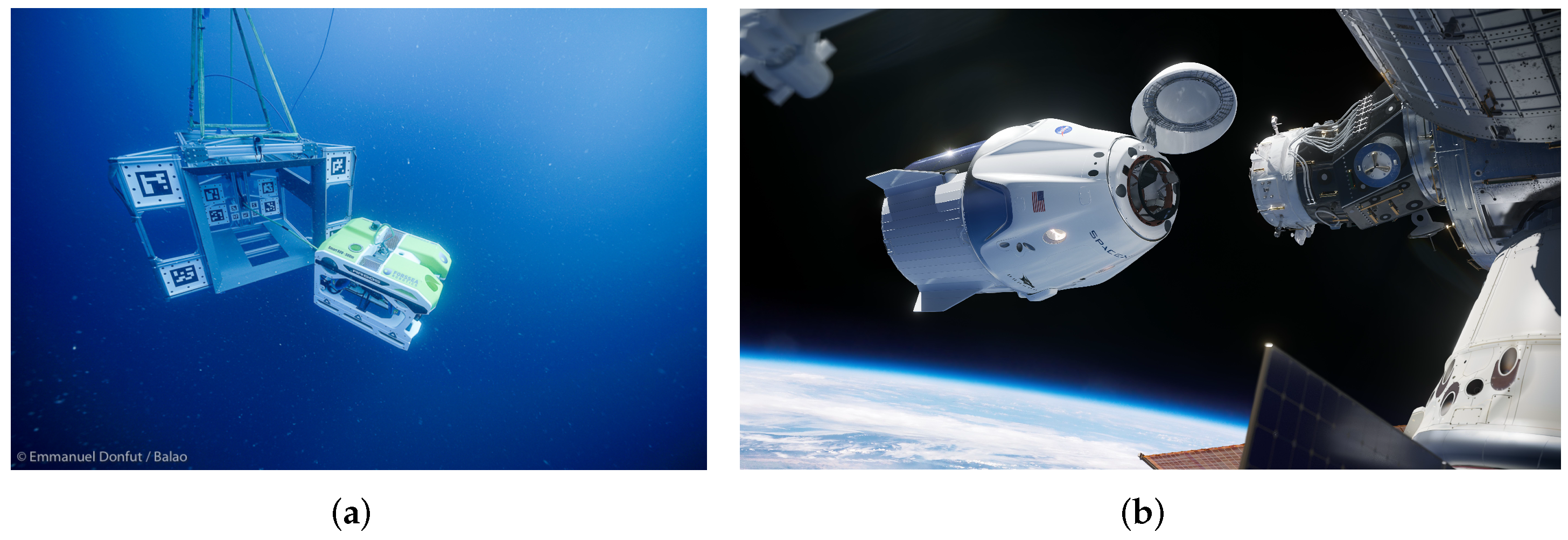Therefore, the primary motivation of our work is to guarantee the success of a mission performed by an autonomous system, such as a robot.

1.2. State of the Art

It is worth noting that methods that prove the outcome of a process have been developed in different domains, illustrating the need for such tools in real-life applications. For example, special programming languages exist to validate software embedded in critical systems [4] or to rigorously simulate and verify hybrid systems [5,6,7]. However, these tools do not fully meet our requirements: they either concentrate on the software part of a system, while we aim to validate the system’s algorithms and dynamics as a whole, on simulating the systems, or they are intended for linear system verification. However, mobile robots are inherently nonlinear.

In [8,9], we proposed a tool that can prove stability of a nonlinear, discrete, continuous, or hybrid system. Thanks to this tool, one can prove that a system will exponentially converge towards an attractor. Uncertainties in the system are tackled using interval analysis. While this tool is powerful when a mission can be formalized as a stability problem, it remains specific. Therefore, we worked on a new approach based on reachability analysis and interval computation to prove feasibility of an autonomous mission.

Reachability analysis consists in proving that a dynamical system can reach a specific area of its state space. Multiple methods exist to analyze a system’s reachable regions [10]. The most intuitive one consists in simulating as many outcomes as possible by considering as many values for the system’s parameters as possible to obtain a rough idea of the system’s behavior with various initial conditions [11,12] (Chapter 8). While easy to understand and implement, this method lacks the mathematical guarantees we seek for our approach. Symbolic reachability analysis can be used: the methods developed in this field allow for this guarantee by enclosing all the possible states of a system inside a mathematical object (usually a set representation that a computer can handle) and studying its evolution in time [13,14,15,16,17,18]. Boxes, zonotopes, or polytopes are generally used to enclose the actual set of possible states for the system, and guaranteed integration algorithms have been developed to propagate these sets in time through a differential equation (or equivalently, a vector field). A promising approach consists in using tubes of trajectories [19], i.e., using a single mathematical object to enclose both state and time information and uncertainties. Each of these approaches has its pros and cons, some being more accurate thanks to the use of more complex sets to the expense of computational power (e.g., zonotopes or polytopes based methods). In contrast, others allow for higher dimensional systems while keeping the required computational power low (some box-based methods). The main difficulty when performing guaranteed computations comes from the balance between accuracy and computational power.

1.3. Contribution

Our method uses tubes to represent the set of trajectories. We then use a guaranteed integration algorithm coupled with contraction mechanisms to narrow this set of trajectories. This allows for the enforcement of differential constraints, given in the form of an autonomous differential equation on a set of trajectories. In a robotics application, a tube obtained using contractors based on external measurements can then be further narrowed using the robot’s behavior described by a differential equation. A similar approach was proposed in [20]: the authors also proposed a contractor for tubes of trajectories based on a guaranteed integration algorithm (using Runge–Kutta approaches, instead of Taylor models). Additionally, they implemented a feature that narrowed the contracted tube even further by using confidence intervals and probability distributions. This approach is interesting since the contraction power can be modulated using application-motivated confidence levels. The obtained results are therefore given with respect to this parameter, which can be challenging to set or interpret.

This paper proposes a guaranteed integration algorithm implemented in a contractor programming framework. This algorithm is our main contribution: we present the theory behind it in the rest of this study, and its implementation can be found online at http://codac.io/slam (accessed on 29 January 2022). We start by presenting the main concepts used in the rest of the article, particularly the original guaranteed integration algorithm and its working principle. Then, we propose a new tube contractor for temporal constraints, expressed as nonlinear differential equations, based on this algorithm. Finally, we detail the different use cases of our contractor through various examples in the field of robotics and autonomous vehicles.

2. Formalization

In this section, we present the notations used in the rest of this article that allow us to formalize a rendezvous problem and represent uncertainties.

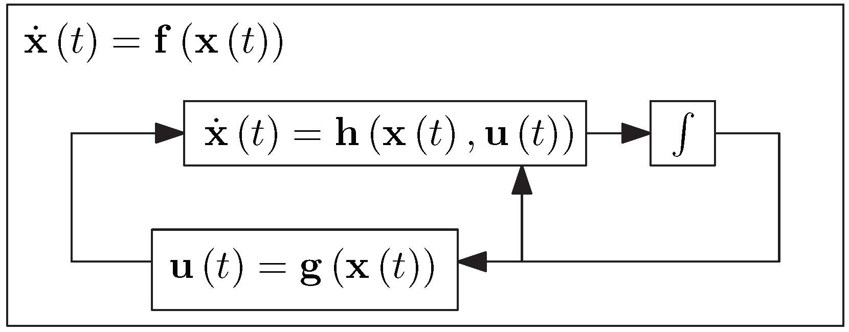
2.1. Formalizing Robots as Dynamical Systems

Mathematically speaking, a robot can be represented as a dynamical system [21,22]. According to [23,24], a dynamical system is a function $\varphi :T\times \mathcal{S}\to \mathcal{S}$ where:

• T is the system’s time set in which the time parameter t evolves;
• $\mathcal{S}$ is the system’s state space containing the system’s state $\mathbf{x}$;
• $\varphi \left(0,·\right)$ is the identity function, $\forall \mathbf{x}\in \mathcal{S},\varphi \left(0,\mathbf{x}\right)=\mathbf{x}$;
• $\varphi \left(t_1,\varphi \left(t_2,\mathbf{x}\right)\right)=\varphi \left(t_1+t_2,\mathbf{x}\right)$ for any $t_1,t_2\in T$ and for any $\mathbf{x}\in \mathcal{S}$.

Usually, $T=\mathbb{R}$ and $\mathcal{S}\subset {\mathbb{R}}^n$. Consider a constant state ${\mathbf{x}}_0\in \mathcal{S}$, then ${\varphi }_{{\mathbf{x}}_0}\left(t\right)$ denotes the flow of the system passing through ${\mathbf{x}}_0$. Consider a constant duration $t_0$, then ${\varphi }_{t_0}\left(\mathbf{x}\right)$ denotes the state transition of duration t of the system.

Now, dynamical systems are closely related to autonomous differential equations of the form

$$\dot{\mathbf{x}}\left(t\right)=\mathbf{f}\left(\mathbf{x}\left(t\right)\right),$$

(1)

where $\mathbf{f}\in {\mathcal{C}}^k\left({\mathbb{R}}^n\right)$ is the evolution function, $t\in \mathbb{R}$ represents time, and $\mathbf{x}\left(t\right)$ is the system’s state at time t. Indeed, Equation (1) has a unique solution ${\varphi }_t\left({\mathbf{x}}_0\right)$ passing through the point ${\mathbf{x}}_0\in {\mathbb{R}}^n$ at time $t=0$, which corresponds to the flow of the associated dynamical system initialized at ${\mathbf{x}}_0$ and $t=0$. This is a consequence of the famous existence and uniqueness theorem [24].

In robotics-related literature [12,21,25], a robot is usually described by a differential equation of the form

$$\dot{\mathbf{x}}\left(t\right)=\mathbf{h}\left(\mathbf{x}\left(t\right),\mathbf{u}\left(t\right)\right),$$

(2)

where $\mathbf{x}\left(t\right)$ is the state of the robot and $\mathbf{u}\left(t\right)$ a control vector. Furthermore, a robot requires a state estimator and a controller to be autonomous. Assuming that the state of the robot is known, e.g., using a state estimator such as a Kalman filter, the control vector is then computed according to a control law of the form

$$\mathbf{u}\left(t\right)=\mathbf{g}\left(\mathbf{x}\left(t\right)\right),$$

(3)

depending on the state $\mathbf{x}$. This control law can be implemented as a PID controller, for example. Therefore, one can combine Equations (2) and (3) to obtain the autonomous system

$$\dot{\mathbf{x}}\left(t\right)=\mathbf{f}\left(\mathbf{x}\left(t\right)\right)=\mathbf{h}\left(\mathbf{x}\left(t\right),\mathbf{g}\left(\mathbf{x}\left(t\right)\right)\right),$$

(4)

also depicted by Figure 2.

Equation (4) describes the behavior of the robot over time, and it can be made as complex as required to match reality. Therefore, one can predict the robot’s state at a later time $t=t_f$ and thus its position by choosing an initial condition $\mathbf{x}\left(t=0\right)={\mathbf{x}}_0$ and integrating over time the corresponding Initial Value Problem (IVP)

$$\left\{\begin{array}{c}\dot{\mathbf{x}}=\mathbf{f}\left(\mathbf{x}\right)\hfill \\ \mathbf{x}\left(t=0\right)={\mathbf{x}}_0\hfill \end{array}\right.$$

(5)

Various methods exist to solve an IVP, the most famous ones being the Euler integration scheme and the Runge–Kutta methods. However, these algorithms cannot handle uncertainties, in particular numerical uncertainties as introduced in the next section. We present in Section 3.1 a so-called guaranteed integration algorithm, whose goal is to solve an uncertain IVP.

2.2. Accounting for System’s Uncertainties

Of course, it would be unrealistic to believe one can predict the actual future state of the robot simply by solving Equation (5). However, if the model is close enough to reality, and if uncertainties are taken into account, one can predict the possible future behaviors of the system. In particular, assuming that the scenario of the mission is specified, and if all uncertainties are taken into account, one could successfully find a subset of ${\mathbb{R}}^n$ containing the actual state of the system at time $t_f$.

To model uncertainties we chose to use intervals of $\mathbb{R}$. Below, we will only introduce the notations used later in this article, and we refer the reader to [26,27,28,29,30] for more details about interval analysis.

An interval of $\mathbb{R}$ is usually denoted by $\left[x\right]=\left[x^{-},x^{+}\right]$. Intervals can be stacked into so-called interval vectors, or boxes, denoted by $\left[\mathbf{x}\right]$, and interval matrices $\left[\mathbf{X}\right]$. We denote by ${\mathbb{IR}}^n$ the set of boxes of ${\mathbb{R}}^n$. Usual arithmetic and set operations are defined for intervals. An interval (a vector or a matrix, respectively) has a mid-point, denoted by $\mathrm{mid}\left(\left[x\right]\right)=\frac{x^{-}+x^{+}}{2}$.

Similarly, one can compute the image of an interval by a function. Rigorously, the image of a set is defined as the set of its members’ images. Since this set may not be an interval anymore, so-called inclusion functions are used to compute an interval enclosure of the image of an interval by a function. However, this introduces the wrapping effect. In Figure 3, $\left[\mathbf{x}\right]\subset {\mathbb{R}}^2$ is an interval vector, $\mathbf{f}\left(\left[\mathbf{x}\right]\right)$ is the image of $\left[\mathbf{x}\right]$ by $\mathbf{f}:{\mathbb{R}}^2\to {\mathbb{R}}^2$, $\left[\mathbf{f}\left(\left[\mathbf{x}\right]\right)\right]$ denotes the minimal inclusion function of $\mathbf{f}$, i.e., it introduces the least wrapping effect, and $\left[\mathbf{f}\right]\left(\left[\mathbf{x}\right]\right)$ denotes a general inclusion function. An example of an inclusion function for $\mathbf{f}$ is the so-called natural inclusion function, which is built using the interval counterparts of the elementary functions (sin, $cos,\cdots$) composing $\mathbf{f}$.

Example 1.

Consider the function $f:x\mapsto \sqrt{x}$ and the interval $\left[x\right]=\left[2,4\right]$. Then $f\left(\left[x\right]\right)=\left[-2,-\sqrt{2}\right]\cup \left[\sqrt{2},2\right]$ is not an interval, hence the need for inclusion functions. The image of $\left[x\right]$ by the minimal inclusion function of f is $\left[-2,2\right]$. The union operation added the interval $\left[-\sqrt{2},\sqrt{2}\right]$ to the set of solutions, which illustrates the wrapping effect.

An interval can be used to enclose the possible values of a quantity. In particular, the state of a system and its parameters can be represented using intervals. What remains necessary is a method allowing to solve an IVP while considering all the possible trajectories of the system induced by its inner uncertainties. Such a method is usually referred to as a guaranteed integration method. We present one of them in Section 3.1.

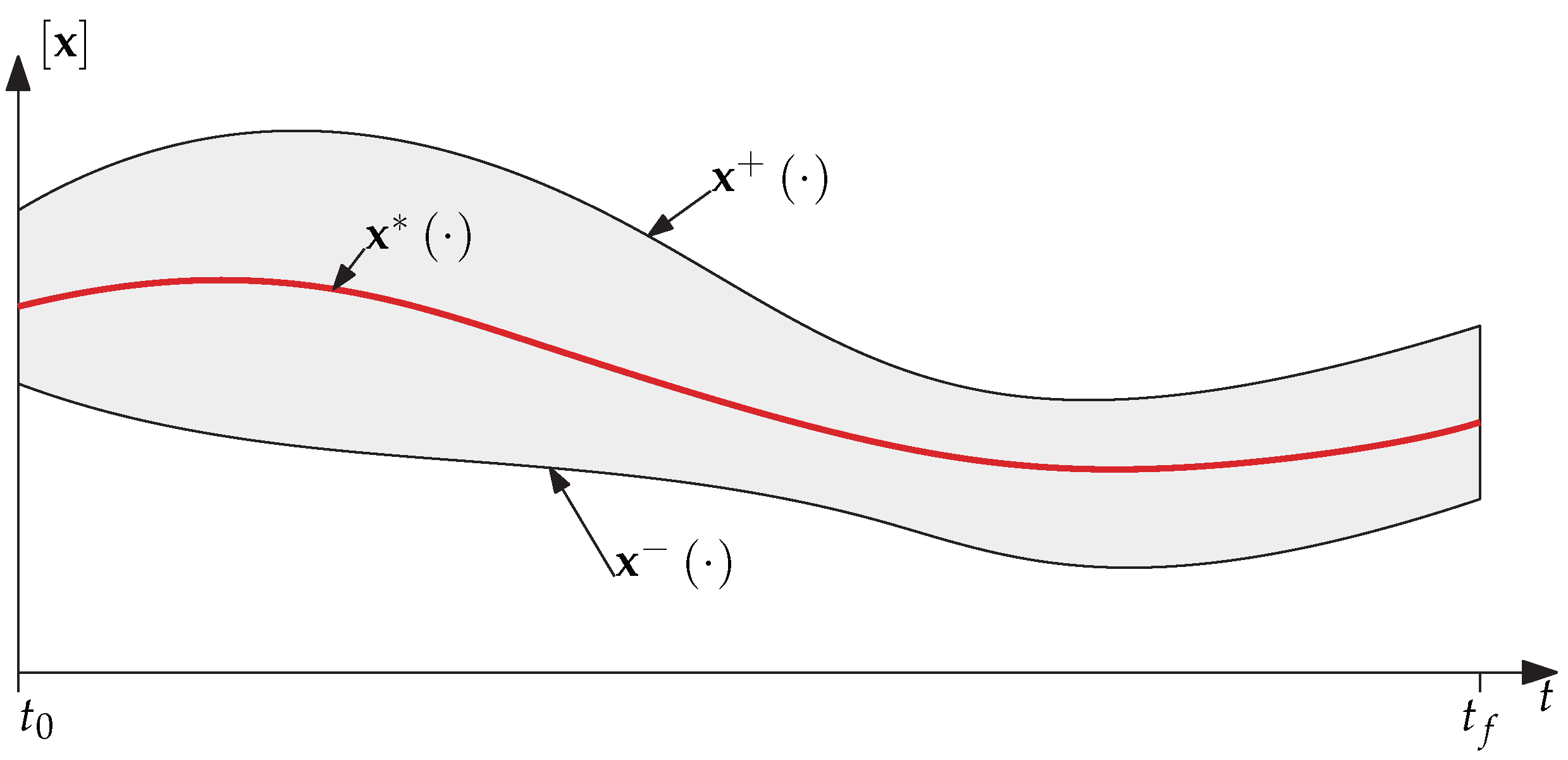
2.3. Tube Arithmetic

Dynamical systems, and consequently robots, describe trajectories in their state space. Therefore, it would be convenient to be able to manipulate “intervals of trajectories” instead of sequences of intervals to represent their state through time. Tube arithmetic was first introduced in [31] and precisely allows for the representation of sets of trajectories of dynamical systems, so-called tubes of trajectories (see Figure 4).

Definition 1

(Tube). A tube $\left[\mathbf{x}\right]\left(·\right):\mathbb{R}\to {\mathbb{IR}}^n$, defined on the time domain $\left[t_0,t_f\right]$, is an interval of trajectories $\left[{\mathbf{x}}^{-}\left(·\right),{\mathbf{x}}^{+}\left(·\right)\right]$ such that $\forall t\in \left[t_0,t_f\right],{\mathbf{x}}^{-}\left(t\right)\le {\mathbf{x}}^{+}\left(t\right)$.

Usual operators can be defined over tubes: let $\left[\mathbf{x}\right]\left(·\right)$ and $\left[\mathbf{y}\right]\left(·\right)$ be two tubes and choose an operator $\diamond \in \left\{+,-,·,/\right\}$. The resulting binary operation between the two tubes is defined as

$$\left[\mathbf{x}\right]\left(·\right)\diamond \left[\mathbf{y}\right]\left(·\right)=\left[\left\{\mathbf{x}\left(·\right)\diamond \mathbf{y}\left(·\right)\in \left(\mathbb{R}\to {\mathbb{R}}^n\right)|\mathbf{x}\left(·\right)\in \left[\mathbf{x}\right]\left(·\right),\mathbf{y}\left(·\right)\in \left[\mathbf{y}\right]\left(·\right)\right\}\right].$$

(6)

Consider a function $\mathbf{f}:{\mathbb{R}}^n\to {\mathbb{R}}^n$. The image of a tube $\left[\mathbf{x}\right]\left(·\right)$ by $\mathbf{f}$ is given by

$$\mathbf{f}\left(\left[\mathbf{x}\right]\left(·\right)\right)=\left[\left\{\mathbf{f}\left(\mathbf{x}\left(·\right)\right)|\mathbf{x}\left(·\right)\in \left[\mathbf{x}\right]\left(·\right)\right\}\right].$$

(7)

This brief introduction to tube arithmetic will be sufficient for the rest of this article. We refer the reader to [32] for more details.

Remark 1.

Note that some trajectories of a tube may not be solutions of an IVP. Mathematically speaking, a trajectory in the sense of tube arithmetic can be seen as a continuous function of time $\mathbf{x}:\mathbb{R}\to {\mathbb{R}}^n$. In the rest of this article, we denote by $\mathbf{x}\left(·\right)$ a trajectory and by $\mathbf{x}\left(t\right)$ a point belonging to the latter, i.e., the evaluation at time t of the function $\mathbf{x}:\mathbb{R}\to {\mathbb{R}}^n$.

2.4. Constraint Programming

Constraint programming is a method that consists in specifying a list of constraints that the elements of a set must verify. The contractor concept is fundamental: it can be seen as an operator that removes elements of the initial set that do not match the constraint.

We refer the reader to [28] for more details about constraint programming applied to interval analysis. What interests us in this article is constraint programming applied to tubes [19,32,33].

Definition 2

(Tube contractor). Consider a constraint $\mathcal{L}$ and a tube $\left[\mathbf{x}\right]\left(·\right)$. A contractor for $\mathcal{L}$ over $\left[\mathbf{x}\right]\left(·\right)$ is an operator $\mathcal{C}:{\mathbb{IR}}^n\to {\mathbb{IR}}^n$ such that

$$\begin{array}{ccc}\hfill \forall t,\mathcal{C}\left(\left[\mathbf{x}\right]\left(·\right)\right)\left(t\right)& \subseteq & \left[\mathbf{x}\right]\left(t\right),\hfill \end{array}$$

(8)

$$\begin{array}{ccc}\hfill \left(\begin{array}{c}\mathcal{L}\left(\mathbf{x}\left(·\right)\right)\\ \mathbf{x}\left(·\right)\in \left[\mathbf{x}\right]\left(·\right)\end{array}\right)& ⟹& \mathbf{x}\left(·\right)\in \mathcal{C}\left(\left[\mathbf{x}\right]\left(·\right)\right).\hfill \end{array}$$

(9)

Equation (8) (monotonicity property) states that the contracted tube is a subset of the original one, and Equation (9) (completeness property) ensures that no trajectory verifying the constraint $\mathcal{L}$ is removed from the original tube.

Now, unlike intervals, tubes inherently embed time information. Two types of contractors can then be defined: static contractors are based on constraints that are time-independent, while temporal contractors impose time constraints, such as differential constraints based on differential equations modeling dynamical systems. The goal of a temporal contractor based on a differential equation is to remove from a tube $\left[\mathbf{x}\right]\left(·\right)$ all the trajectories that are not compatible with the said differential equation.

2.5. Tube Implementation and the Codac Library

Codac [34] is a library for constraint programming over reals, trajectories, and sets. Its development was motivated by mobile robotic problems such as the localization of underwater robots. It proposes various tools to deal with constraints on sets of feasible solutions; several contractors are available and can be used on sets for which the library provides numerical implementations. For instance, various contractors are at hand to compute tubes of trajectories of robots. This allows for the reliable bracketing of a set of trajectories compliant with some sensor measurements and a given differential equation [19,32,35].

The library is available in Python and C++. As an example, one can create a tube $\left[x\right](·)$ over some temporal domain $[t_0,t_f]=[0,10]$, set a restriction on the trajectories at some point: $x\left(t_0\right)\in [-0.1,0.1]$, and define a derivative tube $\left[v\right]\left(t\right)=exp(sin(t\left)\right)+[-0.1,0.1]$ related to a constraint $\dot{x}=v$. The result after contraction, depicted by Figure 5, would be obtained in Python with the following instructions:

tdomain = Interval(0,10)

x = Tube(tdomain, 0.01) # last arg. is a discretization parameter

x.set(Interval(−0.1,0.1), 0.) # x0 \in [−0.1,0.1]

v = Tube(tdomain, 0.01, TFunction("exp(sin(t))+[−0.1,0.1]"))

ctc.deriv.contract(x,v) # a contractor for xdot=v

In Codac, tubes are implemented as a sequence of slices (see Figure 6). The slicing corresponds to the result of a sampling of the tube over time: let $\left[\mathbf{x}\right]\left(·\right)=\left[{\mathbf{x}}^{-}\left(·\right),{\mathbf{x}}^{+}\left(·\right)\right]$ be a tube defined over a time interval $\left[t_0,t_f\right]$, and denote by $\delta >0$ the sampling period. Then, $\left[\mathbf{x}\right]\left(·\right)$ is outer approximated by a sequence of slices denoted by $\left[\mathbf{x}\right]\left(k\right),k\in \mathbb{N}$, such that

$$\left[\mathbf{x}\right]\left(k\right)=\left[k\delta ,\left(k+1\right)\delta \right]\times \left[\underline{{\mathbf{x}}^{-}}\left({\tau }_k\right),\overline{{\mathbf{x}}^{+}}\left({\tau }_k\right)\right],$$

(10)

where ${\tau }_k\in \left[k\delta ,\left(k+1\right)\delta \right]$ and $\underline{{\mathbf{x}}^{-}}\left(t\right)$ and $\overline{{\mathbf{x}}^{+}}\left(t\right)$ are piece-wise constant functions such that

$$\forall t\in \left[t_0,t_f\right],\underline{{\mathbf{x}}^{-}}\left(t\right)\le {\mathbf{x}}^{-}\left(t\right)\le {\mathbf{x}}^{+}\left(t\right)\le \overline{{\mathbf{x}}^{+}}\left(t\right).$$

(11)

A tube (mathematical object $\left[\mathbf{x}\right]\left(·\right)$) implemented in a computer using Codac and evaluated at time t will then return the value of the slice $\left[\mathbf{x}\right]\left(k\right),k\in \mathbb{N}$ where $t\in \left[k\delta ,\left(k+1\right)\delta \right]$. When $t=k\delta$ precisely, the tube is evaluated using the $\left(k-1\right)$th and the kth slices: $\left[\mathbf{x}\right]\left(t\right)\subseteq \left[\mathbf{x}\right]\left(k-1\right)\cap \left[\mathbf{x}\right]\left(k\right)$. $\left[\mathbf{x}\right]\left(k\delta \right)$ is called the input gate of slice k and analogously the output gate of slice $k-1$.

Codac provides a list of static contractors on tubes, such as a contractor ${\mathcal{C}}_{+}(\left[a\right](·),\left[b\right](·),$ $\left[c\right](·))$ for the constraint $\forall t,a\left(t\right)=b\left(t\right)+c\left(t\right)$ with $a(·)\in \left[a\right](·)$, $b(·)\in \left[b\right](·)$, $c(·)\in \left[c\right](·)$. These operators narrow the tubes as much as possible, according to the related constraint and the bounds of the tubes. Other temporal contractors are also available and rely on differential or inter-temporal constraints, such as delays $x\left(t\right)=y(t-\tau )$ or time uncertainties: $y=x\left(t_1\right)$, $t_1\in \left[t_1\right]$. Since this approach does not remove any feasible solution from the sets, the contractors can be easily combined to deal with realistic problems that are usually difficult to solve. For instance, Codac is used to solve Simultaneous Localization And Mapping (SLAM) problems with strong uncertainties and nonlinear equations. See, for instance: http://codac.io/slam (accessed on 29 January 2022).

3. Guaranteed Integration: A Constraint Programming Approach

Now that we introduced the main concepts used in this article, we will present the main contribution of this work: the implementation of a temporal contractor for tubes based on a famous guaranteed integration method proposed by Lohner in [36]. We start by introducing the latter, providing a simple implementation, and then we propose a contractor based on this method to deal with differential constraints. For more information about guaranteed integration, we refer the reader to [29,30].

3.1. Lohner Algorithm

Many guaranteed integration algorithms have been proposed over the last 60 years. Here, we chose to present a method from which most current algorithms originate. Lohner’s algorithm is based on a temporal Taylor decomposition with Lagrange remainder, centered form evaluation of inclusion functions, and non-axis-aligned boxes of ${\mathbb{R}}^n$. For a complete derivation of this algorithm, we refer the reader to [36] and for more details to [37,38].

Consider an IVP, such as the one described by Equation (5), where ${\mathbf{x}}_0\in \left[{\mathbf{x}}_0\right]$, and denote by $\varphi \left(t,\mathbf{x}\right)$ the associated dynamical system. Denote by $\delta$ the integration step size and by $\left[{\mathbf{x}}_k\right]$ the enclosure of the system’s state at time $t_k=k\delta$. To solve this problem, Lohner proceeds as follows (see Figure 7):

• Find a global enclosure $\left[{\tilde{\mathbf{x}}}_k\right]$ for the system’s trajectories over the time interval $\left[t_k,t_{k+1}\right]$;
• Using $\left[{\tilde{\mathbf{x}}}_k\right]$, find an enclosure for the state at time $t_{k+1}$, i.e., $\left[{\mathbf{x}}_{k+1}\right]$.

The first step is performed by a so-called First Order Enclosure algorithm: it is based on the Picard–Lindelöf operator and Banach’s fixed-point theorem (see [27,39,40] for more details). Below, we give a simple implementation of this algorithm and illustrate its working principle in Figure 8.

Algorithm 1 takes three parameters as inputs: the state’s enclosure $\left[{\mathbf{x}}_k\right]$ at time $t_k$, a reduction parameter $\mu$, an inflation parameter $ϵ$, and a maximum number of iterations $i_{max}$. The input/output parameter $\delta$ denotes the integration step size and can be modified. It computes the global enclosure $\left[{\tilde{\mathbf{x}}}_k\right]$, i.e., the box containing all possible trajectories of the system in the time interval $\left[t_k,t_{k+1}\right]$.

Algorithm 2 integrates $\varphi \left(t,\mathbf{x}\right)$ over N integration steps of size $\delta$. It uses the result of Algorithm 1 to compute the state enclosure at each integration step. This algorithm is based on a second-order Taylor decomposition of $\varphi \left(t,\mathbf{x}\right)$ and requires the computation of the Jacobian matrix of $\mathbf{f}$, denoted by ${\mathbf{J}}_{\mathbf{f}}$. It uses the global enclosure to outer-approximate the Lagrange remainder of the decomposition. The state enclosure is represented inside the algorithm by a tilted box ${\mathbf{B}}_{k+1}\left[{\mathbf{r}}_{k+1}\right]$ (${\mathbf{B}}_{k+1}$ being an orthogonal matrix and $\left[{\mathbf{r}}_{k+1}\right]$ a box of ${\mathbb{R}}^n$) centered in ${\widehat{\mathbf{x}}}_{k+1}$, to avoid including too much wrapping effect in the computations.

To sum up:

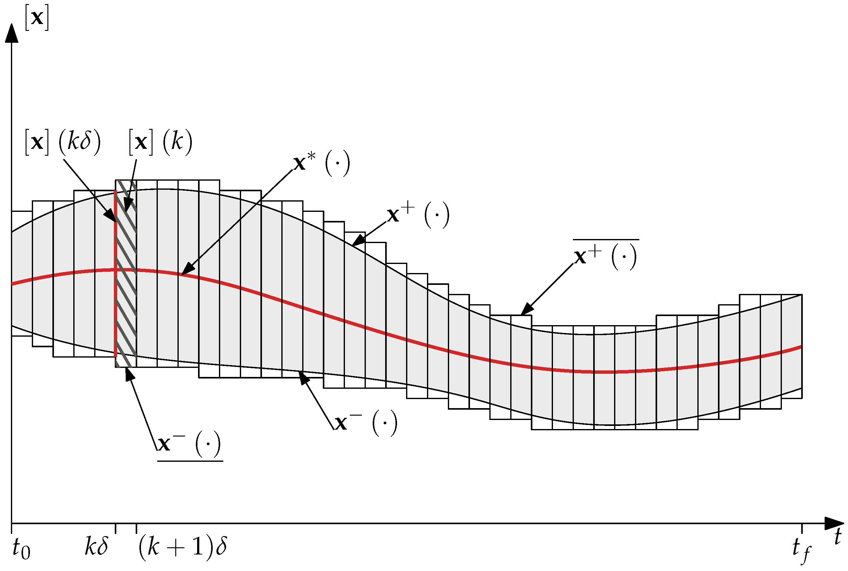
• Given an initial state enclosure $\left[{\mathbf{x}}_0\right]$, Algorithm 2 can compute a sequence of boxes $\left[{\mathbf{x}}_k\right]$ that contains the system’s state at time $t_k=k\delta$;
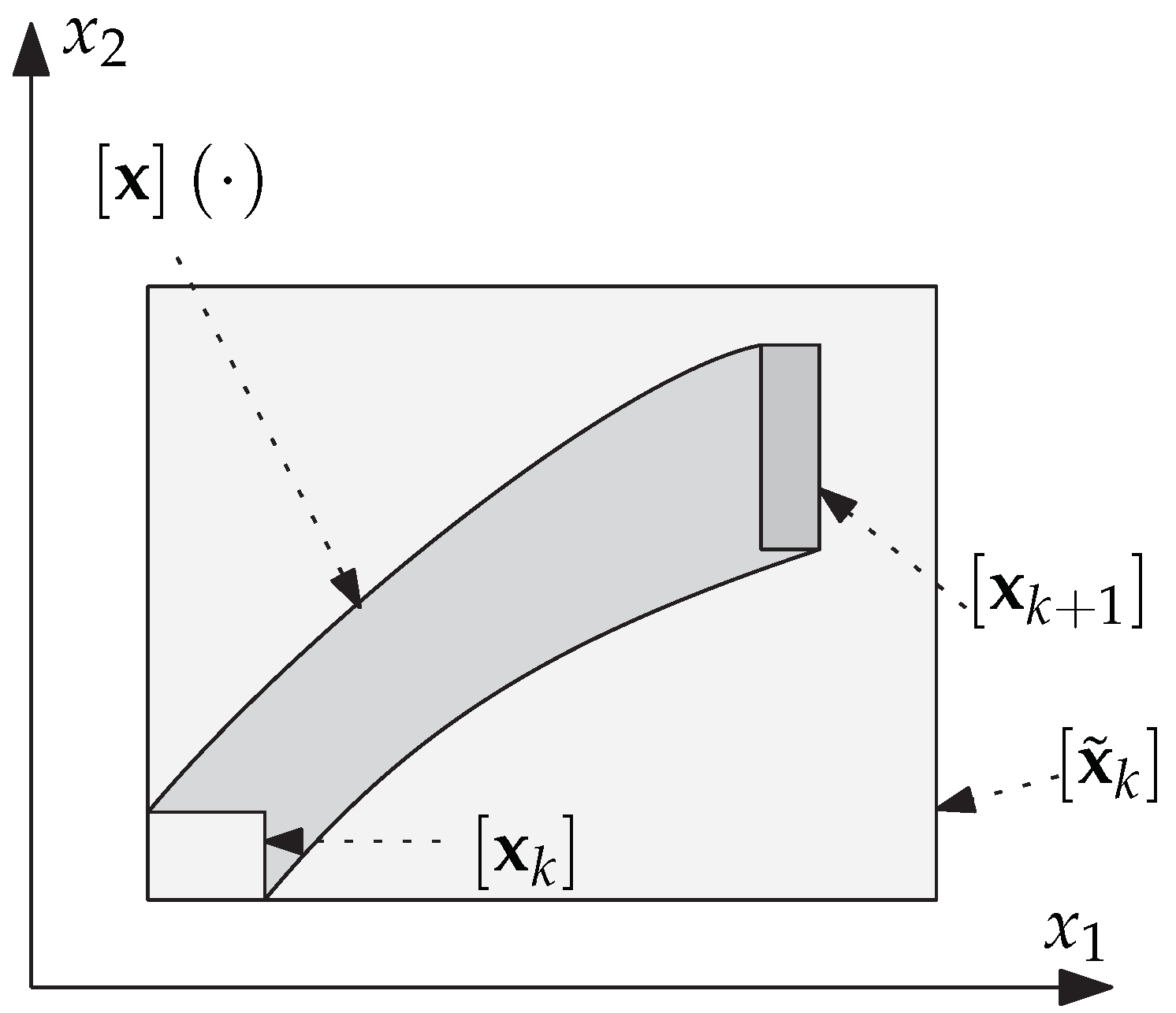
• For all $k\ge 0$, the enclosure $\left[{\mathbf{x}}_k\right]$ is actually represented by a tilted box in Algorithm 2: $\left[{\mathbf{x}}_k\right]={\widehat{\mathbf{x}}}_k+{\mathbf{B}}_k\left[{\mathbf{r}}_k\right]$, where both $\left[{\mathbf{x}}_k\right]$ and $\left[{\mathbf{r}}_k\right]$ represent the system’s state enclosure, respectively, in the canonical basis and in the one defined by the orthogonal matrix ${\mathbf{B}}_k$;
• Algorithm 2 computes at each time step k the global enclosure $\left[{\tilde{\mathbf{x}}}_k\right]$, such that for all $t\in \left[t_k,t_{k+1}\right]$ and for all ${\mathbf{x}}_k\in \left[{\mathbf{x}}_k\right]$, $\varphi \left(t-t_k,{\mathbf{x}}_k\right)\in \left[{\tilde{\mathbf{x}}}_k\right]$.

Algorithm 1GlobalEnclosure (in: $\left[{\mathbf{x}}_k\right]$, $ϵ$, $\mu$, $i_{max}$, out: $\left[{\tilde{\mathbf{x}}}_k\right]$, inout: $\delta$)
$\left[{\tilde{\mathbf{x}}}_k^0\right]\leftarrow \left[{\mathbf{x}}_k\right]$
2: $\left[{\tilde{\mathbf{x}}}_k^1\right]\leftarrow \left[{\mathbf{x}}_k\right]+\left[0,\delta \right]\mathbf{f}\left(\left[{\tilde{\mathbf{x}}}_k^0\right]\right)$
$i\leftarrow 0$
4: while$\left[{\tilde{\mathbf{x}}}_k^1\right]\neg \subseteq \left[{\tilde{\mathbf{x}}}_k^0\right]$do
$i\leftarrow i+1$	Increase the number of iterations
6:    if $i\ge i_{max}$ then
$i\leftarrow 0$	Reset the iteration counter
8:      $\delta \leftarrow \mu ·\delta$	Reduce the time step by a factor$\mu$
	Reset the a priori estimates
10:      $\left[{\tilde{\mathbf{x}}}_k^0\right]\leftarrow \left[{\mathbf{x}}_k\right]$
$\left[{\tilde{\mathbf{x}}}_k^1\right]\leftarrow \left[{\mathbf{x}}_k\right]+\left[0,\delta \right]\mathbf{f}\left(\left[{\tilde{\mathbf{x}}}_k^0\right]\right)$
12:    end if
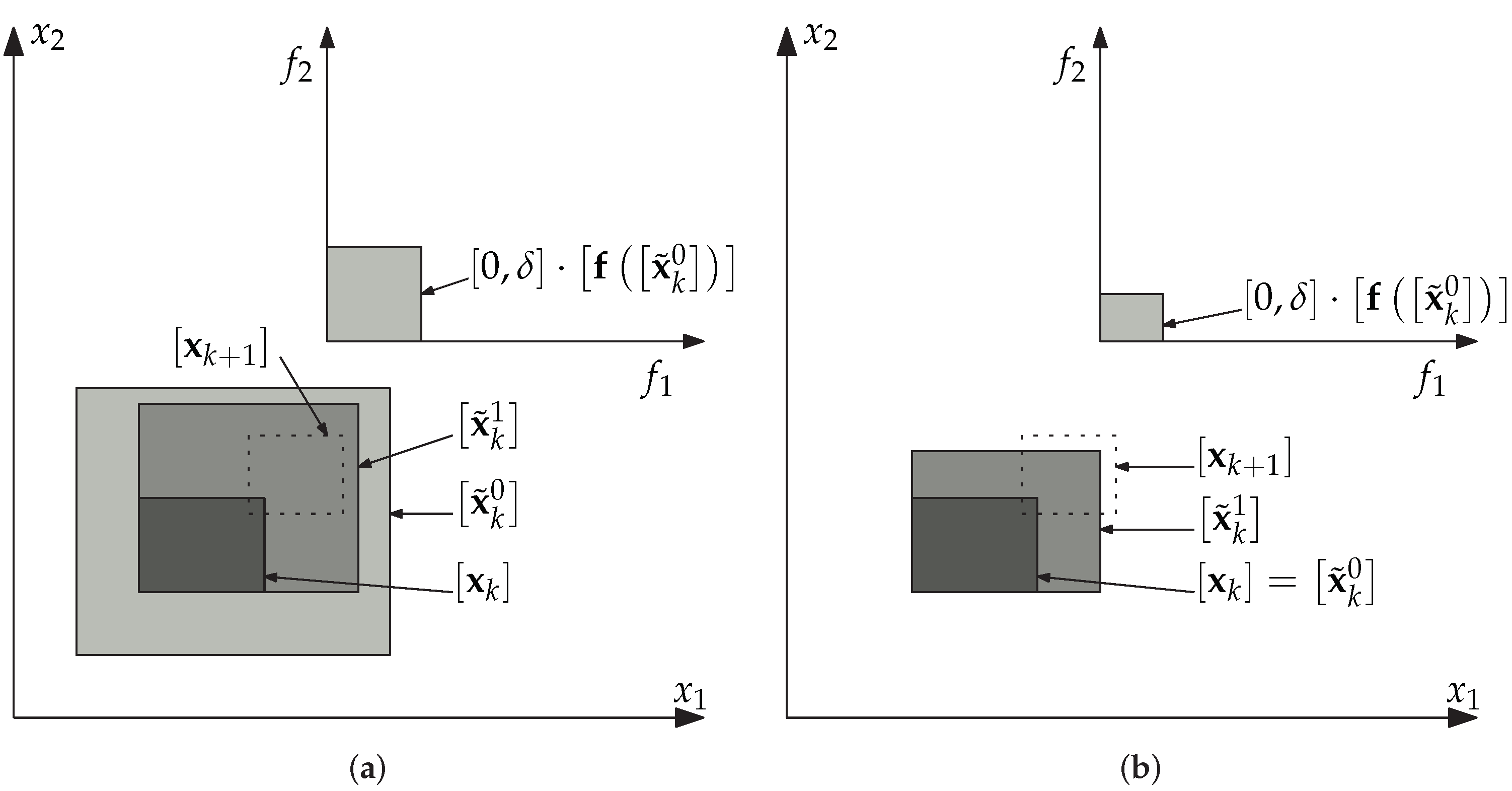
$\left[{\tilde{\mathbf{x}}}_k^0\right]\leftarrow \left(1+ϵ\right)\left[{\tilde{\mathbf{x}}}_k^1\right]-ϵ\left[{\tilde{\mathbf{x}}}_k^1\right]$	Inflate the a priori estimate
14:    $\left[{\tilde{\mathbf{x}}}_k^1\right]\leftarrow \left[{\mathbf{x}}_k\right]+\left[0,\delta \right]\mathbf{f}\left(\left[{\tilde{\mathbf{x}}}_k^0\right]\right)$	Compute the new a priori estimate
end while
16: return$\left[{\tilde{\mathbf{x}}}_k^0\right]$

Algorithm 2SimpleLohner (in: $\left[{\mathbf{x}}_0\right]$, $\delta$, N, out: $\left[{\mathbf{x}}_N\right]$)
${\widehat{\mathbf{x}}}_0\leftarrow \mathrm{mid}\left(\left[{\mathbf{x}}_0\right]\right)$	initialisation
2: $\left[{\mathbf{z}}_0\right]\leftarrow \left[{\mathbf{x}}_0\right]-{\widehat{\mathbf{x}}}_0$
${\mathbf{m}}_0\leftarrow \mathrm{mid}\left(\left[{\mathbf{z}}_0\right]\right)=\mathbf{0}$
4: $\left[{\mathbf{r}}_0\right]\leftarrow \left[{\mathbf{z}}_0\right]-{\mathbf{m}}_0=\left[{\mathbf{z}}_0\right]$
${\mathbf{B}}_0=\mathbf{I}$
6: for$k=0$to$N-1$do
$\left[{\mathbf{A}}_k\right]\leftarrow \mathbf{I}+\delta \left[{\mathbf{J}}_{\mathbf{f}}\right]\left(\left[{\mathbf{x}}_k\right]\right)$
8:    $\left[{\tilde{\mathbf{x}}}_k\right]\leftarrow$GlobalEnclosure$\left(\left[{\mathbf{x}}_k\right]\cdots \right)$ see Algorithm 1 (for the sake of simplicity, we consider that $\delta$ does not change during the evaluation of GlobalEnclosure)
$\left[{\mathbf{z}}_{k+1}\right]\leftarrow {\displaystyle \frac{{\delta }^2}{2}}\left[{\mathbf{J}}_{\mathbf{f}}\right]\left(\left[{\tilde{\mathbf{x}}}_k\right]\right)\left[\mathbf{f}\right]\left(\left[{\tilde{\mathbf{x}}}_k\right]\right)$
10:    ${\mathbf{m}}_{k+1}\leftarrow \mathrm{mid}\left(\left[{\mathbf{z}}_{k+1}\right]\right)$
${\mathbf{B}}_{k+1}\leftarrow \mathrm{Qr}\left(\mathrm{mid}\left(\left[{\mathbf{A}}_k\right]{\mathbf{B}}_k\right)\right)$	orthogonal part of the QR factorisation
12:    $\left[{\mathbf{r}}_{k+1}\right]\leftarrow \left({\mathbf{B}}_{k+1}^{-1}\left[{\mathbf{A}}_k\right]{\mathbf{B}}_k\right)\left[{\mathbf{r}}_k\right]+{\mathbf{B}}_{k+1}^{-1}\left(\left[{\mathbf{z}}_{k+1}\right]-{\mathbf{m}}_{k+1}\right)$
${\widehat{\mathbf{x}}}_{k+1}\leftarrow {\widehat{\mathbf{x}}}_k+\delta \mathbf{f}\left({\widehat{\mathbf{x}}}_k\right)+{\mathbf{m}}_{k+1}$
14:    $\left[{\mathbf{x}}_{k+1}\right]\leftarrow {\widehat{\mathbf{x}}}_{k+1}+{\mathbf{B}}_{k+1}\left[{\mathbf{r}}_{k+1}\right]$
end for
16: return$\left[{\mathbf{x}}_N\right]$

3.2. Lohner Contractor

This section presents our main contribution: merging the guaranteed integration algorithm and contractor programming. We use the contractor programming paradigm to remove trajectories that would be unfeasible according to a given differential constraint (i.e., an autonomous differential equation) from a tube of trajectories. To check whether a trajectory is feasible, we use Lohner’s algorithm and the information contained in the tube’s implementation, as explained below.

Remark 2.

An approach merging contractor programming with a guaranteed integration algorithm is not new, as it can be found in [41,42], for example. However, additionally to thoroughly presenting our work, we provide an open-source implementation of our contractor in the library Codac, as well as examples of applications. The reader can then easily reuse our contractor, coupled with others also provided by Codac, to solve problems in various fields of application.

Consider a tube $\left[\mathbf{x}\right]\left(·\right)$ enclosing the state of a system defined by an autonomous differential equation $\dot{\mathbf{x}}=\mathbf{f}\left(\mathbf{x}\right)$ over a time interval $\left[t_0,t_f\right]$. Assume that the tube is represented by slices of width $\delta$, and let us define the sequence $t_k=k\delta$. Then, one can notice that:

• $\left[\mathbf{x}\right]\left(t_0\right)$ can be seen as the input gate of slice 0 and the system’s initial condition, i.e., forming an IVP;
• $\left[\mathbf{x}\right]\left(t_k\right)$ can be interpreted as the kth slice’s input gate, the $\left(k-1\right)$th slice’s output gate, and the system’s state enclosure at time $t_k$;
• $\left[\mathbf{x}\right]\left(k\right)$ is the kth slice of $\left[\mathbf{x}\right]\left(·\right)$, thus containing all the system trajectories over the time interval $\left[t_k,t_{k+1}\right]$. $\left[\mathbf{x}\right]\left(k\right)$ can therefore be seen as a global enclosure for the system over $\left[t_k,t_{k+1}\right]$.

Let us now explain how we implement our contractor, using Algorithm 2:

• Assume that we initialize the algorithm with the initial box $\left[\mathbf{x}\right]\left(t_0\right)$;
• Then, all the system trajectories during the time interval $\left[t_k,t_{k+1}\right]$ must be contained both in the slice $\left[\mathbf{x}\right]\left(k\right)$ and in the global enclosure $\left[{\tilde{\mathbf{x}}}_k\right]$;
• Consider the kth slice: at time $t_k$, the system’s state is enclosed by $\left[\mathbf{x}\right]\left(t_k\right)$, and at time $t_{k+1}$, it is enclosed both in the slice’s output gate $\left[\mathbf{x}\right]\left(t_{k+1}\right)$ and in the box $\left[{\mathbf{x}}_{k+1}\right]$ computed by Algorithm 2;
• Finally, we have $\left[{\mathbf{x}}_k\right]={\widehat{\mathbf{x}}}_k+{\mathbf{B}}_k\left[{\mathbf{r}}_k\right]$.

Algorithm 3 is the implementation of our Lohner contractor for tubes of trajectories, and it is illustrated by Figure 9. Figure 9a is a scheme representing a 1D tube, the input of the Lohner contractor. Figure 9b–f illustrate the contraction of the initial tube by our algorithm, in forward (increasing time) and backward (decreasing time) modes. This contraction is performed thanks to an arbitrary differential equation. In particular, one should notice that the contraction of a slice is performed using the latter’s input gate. This demonstrates the interest of our contractor. Let us imagine that the initial tube has been obtained using a contractor enforcing state measurement constraints; our contractor can then be used to contract this tube with respect to the system model.

Algorithm 3${\mathcal{C}}_{Lohner}$ (inout: $\left[\mathbf{x}\right]\left(·\right)$)
Initialisation:
2: $\left[{\mathbf{x}}_0\right]\leftarrow \left[\mathbf{x}\right]\left(t_0\right)$
${\widehat{\mathbf{x}}}_0\leftarrow \mathrm{mid}\left(\left[{\mathbf{x}}_0\right]\right)$
4: $\left[{\mathbf{z}}_0\right]\leftarrow \left[{\mathbf{x}}_0\right]-{\widehat{\mathbf{x}}}_0$
${\mathbf{m}}_0\leftarrow \mathrm{mid}\left(\left[{\mathbf{z}}_0\right]\right)=\mathbf{0}$
6: $\left[{\mathbf{r}}_0\right]\leftarrow \left[{\mathbf{z}}_0\right]-{\mathbf{m}}_0=\left[{\mathbf{z}}_0\right]$
${\mathbf{B}}_0=\mathbf{I}$
8: Main loop:
for $k=0$ to$\frac{t_f}{\delta }$ do
10:    Lohner integration:	see Algorithm 2
$\left[{\mathbf{A}}_k\right]\leftarrow \mathbf{I}+\delta \left[{\mathbf{J}}_{\mathbf{f}}\right]\left(\left[{\mathbf{x}}_k\right]\right)$
12:    $\left[{\tilde{\mathbf{x}}}_k\right]\leftarrow$GlobalEnclosure$\left(\left[{\mathbf{x}}_k\right]\cdots \right)$ see Algorithm 1 (for the sake of simplicity, we consider that $\delta$ does not change during the evaluation of GlobalEnclosure)
$\left[{\mathbf{z}}_{k+1}\right]\leftarrow {\displaystyle \frac{{\delta }^2}{2}}\left[{\mathbf{J}}_{\mathbf{f}}\right]\left(\left[{\tilde{\mathbf{x}}}_k\right]\right)\left[\mathbf{f}\right]\left(\left[{\tilde{\mathbf{x}}}_k\right]\right)$
14:    ${\mathbf{m}}_{k+1}\leftarrow \mathrm{mid}\left(\left[{\mathbf{z}}_{k+1}\right]\right)$
${\mathbf{B}}_{k+1}\leftarrow \mathrm{Qr}\left(\mathrm{mid}\left(\left[{\mathbf{A}}_k\right]{\mathbf{B}}_k\right)\right)$	orthogonal part of the QR factorization
16:    $\left[{\mathbf{r}}_{k+1}\right]\leftarrow \left({\mathbf{B}}_{k+1}^{-1}\left[{\mathbf{A}}_k\right]{\mathbf{B}}_k\right)\left[{\mathbf{r}}_k\right]+{\mathbf{B}}_{k+1}^{-1}\left(\left[{\mathbf{z}}_{k+1}\right]-{\mathbf{m}}_{k+1}\right)$
${\widehat{\mathbf{x}}}_{k+1}\leftarrow {\widehat{\mathbf{x}}}_k+\delta \mathbf{f}\left({\widehat{\mathbf{x}}}_k\right)+{\mathbf{m}}_{k+1}$
18:    $\left[{\mathbf{x}}_{k+1}\right]\leftarrow {\widehat{\mathbf{x}}}_{k+1}+{\mathbf{B}}_{k+1}\left[{\mathbf{r}}_{k+1}\right]$
Tube contraction:
20:    $\left[{\mathbf{x}}_{k+1}\right]\leftarrow \left[{\mathbf{x}}_{k+1}\right]\cap \left[\mathbf{x}\right]\left(t_{k+1}\right)$	contracts$\left[{\mathbf{x}}_{k+1}\right]$
${\widehat{\mathbf{x}}}_{k+1}\leftarrow \mathrm{mid}\left(\left[{\mathbf{x}}_{k+1}\right]\right)$	adjusts the center of the tilted box
22:    $\left[{\mathbf{r}}_{k+1}\right]\leftarrow \left[{\mathbf{r}}_{k+1}\right]\cap \left({\mathbf{B}}_{k+1}^{-1}·\left(\left[{\mathbf{x}}_{k+1}\right]-{\widehat{\mathbf{x}}}_{k+1}\right)\right)$	contracts uncertainties in tilted frame
$\left[\mathbf{x}\right]\left(t\right)=\left\{\begin{array}{cc}\left[\mathbf{x}\right]\left(t\right)\cap \left[{\tilde{\mathbf{x}}}_k\right]\hfill & \mathrm{if}t\in \left[t_k,t_{k+1}\right[;\hfill \\ \left[\mathbf{x}\right]\left(t\right)\cap \left[{\mathbf{x}}_{k+1}\right]\hfill & \mathrm{if}t=t_{k+1}.\hfill \end{array}\right.$	contracts the slice and the output gate
24: end for

Proposition 1.

Consider a dynamical system described by $\dot{\mathbf{x}}=\mathbf{f}\left(\mathbf{x}\right)$, and a tube of trajectories $\left[\mathbf{x}\right]\left(·\right)$ defined over $\left[t_0,t_f\right]$. Then the operator ${\mathcal{C}}_{Lohner}$ is a contractor for $\left[\mathbf{x}\right]\left(·\right)$ over $\left[t_0,t_f\right]$.

Proof. 

The monotonicity property (Equation (8)) comes from the 23rd line of Algorithm 3: for all $t\in \left[t_k,t_{k+1}\right]$, we have

$$\begin{array}{ccc}\hfill {\mathcal{C}}_{Lohner}\left(\left[\mathbf{x}\right]\left(·\right)\right)\left(t\right)& =& \left[\mathbf{x}\right]\left(t\right)\cap \left\{\begin{array}{cc}\left[{\tilde{\mathbf{x}}}_k\right]\hfill & \mathrm{if}t\ne t_k;\hfill \\ \left[{\mathbf{x}}_k\right]\hfill & \mathrm{if}t=t_k.\hfill \end{array}\right.\hfill \\ & \subset & \left[\mathbf{x}\right]\left(t\right)\hfill \end{array}$$

The completeness property comes from lines 20 and 23. Indeed, the state at time $t_{k+1}$ is contained both in $\left[{\mathbf{x}}_{k+1}\right]$ (according to Algorithm 2) and in $\left[\mathbf{x}\right]\left(t_{k+1}\right)$ (according to the initial tube). Furthermore, the system’s trajectories over the time interval $\left[t_k,t_{k+1}\right]$ are contained both in $\left[\mathbf{x}\right]\left(k\right)$ and in $\left[{\tilde{\mathbf{x}}}_k\right]$. Therefore, no solution verifying both the differential constraint and the initial tube is removed.    □

Remark 3.

Once the tube has been contracted from its first to last slice (forward mode), the contractor can be used in the reverse direction (backward mode) simply by considering $\dot{\mathbf{x}}=-1·\mathbf{f}\left(\mathbf{x}\right)$ as a dynamical system. ${\mathcal{C}}_{Lohner}$ can be composed with itself or other tube contractors, multiple times if necessary (see [28] for more details about contractor composition).

Remark 4.

The Lohner contractor takes a tube as an input. Its complexity therefore depends both on its time span (i.e., the number of slices) and its dimension. Let us recall that m denotes the number of slices, and n denotes the tube’s dimension. ${\mathcal{C}}_{Lohner}$ has $O\left(m\right)$ time complexity and $O\left(n^3\right)$ dimension complexity. Indeed, the most complex operations in the algorithm are matrix products, inversions, and QR decompositions.

The Lohner contractor has been added to the Codac library, and its documentation can be found online at http://codac.io/lohner (accessed on 29 January 2022). It has been implemented both in Python and in C++ and allows for forward and backward contractions.

4. Applications

This section aims to illustrate our Lohner contractor with various examples. The first one is a one-dimensional differential equation. Although simple, this equation amplifies the wrapping effect when dealt with using a simpler differential contractor, justifying the need for ours. The second example illustrates how our contractor could be used to solve a robotics-related problem.

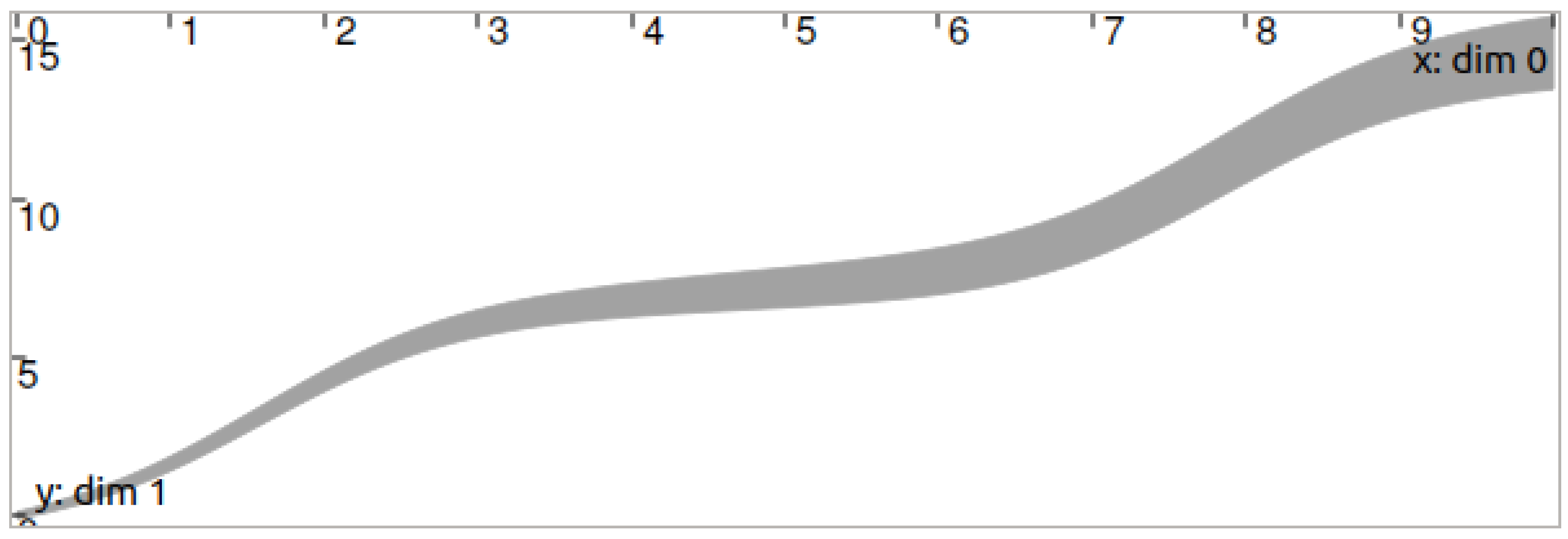
4.1. Simple Illustrating Example

As a first example, let us consider the one-dimensional system given by

$$\dot{x}=-sin\left(x\right).$$

(12)

Let us take $\left[x_0\right]=\left[0.9,1.1\right]$ as an initial state, thanks to which we initialize the tube $\left[x\right]\left(·\right)$ with

$$\left[x\right]\left(t\right)=\left\{\begin{array}{cc}\left[x_0\right]\hfill & \mathrm{if}t=0;\hfill \\ \left[-\infty ,\infty \right]\hfill & \mathrm{otherwise}.\hfill \end{array}\right.$$

Now, we compute ${\mathcal{C}}_{Lohner}\left(\left[x\right]\left(·\right)\right)$, and we obtain Figure 10, where the tube was contracted using slices of duration $\delta =0.1$.

Let us now compare this result with a tube obtained using the Picard contractor ${\mathcal{C}}_{Picard}$ (see Figure 11). The latter is also a differential contractor for tubes, simply based on the Picard–Lindelhöf operator (we refer the reader to [38] (Chapter 4) for an extensive presentation of the latter).

The Picard contractor, which does not take into account the derivatives of the differential equation, cannot appropriately deal with the wrapping effect, and the contraction of the tube diverges. Both in Figure 10 and Figure 11, the blue trajectories correspond to the actual trajectories of a distribution of points contained inside the initial state $\left[x_0\right]$. The goal behind representing these trajectories is to visualize the difference between the tube contracted by the two contractors and an approximation of the system’s trajectory when initialized in $\left[x_0\right]$.

4.2. Underwater Docking Mission Feasibility

Our second example demonstrates a possible usage of the Lohner contractor for a real-life problem: an autonomous underwater robot has to dock inside a docking station $\left[\mathbf{d}\right]$ at a given time T. The robot can localize itself with respect to the latter and measure its velocity. It is controlled by a velocity controller, which drives it along a vector field, attracting the robot to the docking station. To dock successfully, the robot needs to arrive right in front of the station’s entrance, with a certain velocity. Finally, currents are quite strong around the docking station. The goal is to find the area ${\mathcal{D}}^{+}$ inside which it is mathematically proven that the robot will dock afterwards, despite measurement errors and current-induced drift.

4.2.1. Modeling the Robot as a Dynamical System

Modeling the dynamics of an underwater robot can be quite complex, as the involved external forces are strongly nonlinear (see [21] for more details). In this paper, we propose a simplified model for an autonomous ROV (Remotely Operated Vehicle). We assume that the ROV is equipped with an accurately performing attitude controller, which keeps it aligned in the right direction to dock inside the docking station. We also assume that the ROV is holonomic, i.e., it can move in any direction. Finally, we limit ourselves to the XY plane. These design constraints are enforced not because they would complexify the equations but because a six-dimensional (surge, sway, heave, roll, pitch, and yaw) state would be much harder to visualize. Furthermore, while our contractor’s performance has a polynomial complexity with respect to the state’s dimension (because of matrix products), we bisect the initial state to get a better approximation of ${\mathcal{D}}^{+}$ in the form of a paving of the state space, leading to an algorithm with exponential complexity. Note that the latter is not a problem, since approximating ${\mathcal{D}}^{+}$ is a problem that ought to be solved offline; therefore, computational power is available.

We then define the system’s state as $\mathbf{x}=\left(x,y,v_x,v_y\right)$, where the first two elements are the ROV’s position and the two last are the ROV’s velocity. We denote the current’s velocity by $\mathbf{c}=\left(c_x,c_y\right)$. Let us now introduce the equations describing the system dynamics (Equation (13)), the system’s controller (Equation (14)), and the steering vector field (Equation (15)), as follows:

$$\begin{array}{ccc}\hfill \dot{\mathbf{x}}\left(t\right)=\mathbf{h}\left(\mathbf{x}\left(t\right),\mathbf{u}\left(t\right)\right)& =& \left(\begin{array}{c}{v}_x\\ v_y\\ u_x-k_{fx}\left(v_x-c_x\right)\left|v_x-c_x\right|\\ u_y-k_{fy}\left(v_y-c_y\right)\left|v_y-c_y\right|\end{array}\right),\hfill \end{array}$$

(13)

$$\begin{array}{ccc}\hfill \mathbf{u}\left(t\right)=\mathbf{g}\left({\mathbf{v}}_d\left(t\right),\mathbf{x}\left(t\right)\right)& =& \left(\begin{array}{c}{k}_{px}\left(v_{dx}-{\overline{v}}_x\right)+k_{fx}\left({\overline{v}}_x-{\overline{c}}_x\right)\left|{\overline{v}}_x-{\overline{c}}_x\right|\\ k_{py}\left(v_{dy}-{\overline{v}}_y\right)+k_{fy}\left({\overline{v}}_y-{\overline{c}}_y\right)\left|{\overline{v}}_y-{\overline{c}}_y\right|\end{array}\right),\hfill \end{array}$$

(14)

$$\begin{array}{ccc}\hfill {\mathbf{v}}_d\left(t\right)=\mathbf{j}\left(\mathbf{x}\left(t\right)\right)& =& \left(\begin{array}{c}{v}_0\left(1-{tanh}^2\left(\overline{y}\right)\right)\\ -v_{0}tanh\left(\overline{y}\right)\end{array}\right),\hfill \end{array}$$

(15)

where $k_{fx},k_{fy}$ are damping coefficients, $k_{px},k_{py}$ are the proportional controller’s coefficients, $v_0$ is the desired velocity, and $\overline{·}$ denotes a measured variable, i.e., a state variable with added uncertainty.

Equation (13) describes the dynamics of the robot in a plane, $u_x$ and $u_y$ being the accelerations imposed by the robot’s thrusters and the remaining term corresponding to a friction force. Equation (14) describes the proportional controller driving the robot along the vector field ${\overrightarrow{v}}_d$ and pre-compensating the effects of the water currents. Finally, Equation (15) describes the vector field drawn in Figure 12a. These equations can be composed into an autonomous differential equation of the form $\dot{\mathbf{x}}=\mathbf{f}\left(\mathbf{x}\right)$.

4.2.2. Computing ${\mathcal{D}}^{+}$

To compute an approximation of ${\mathcal{D}}^{+}$, we start taking a large initial box $\left[{\mathbf{x}}_0\right]$, where we believe that the robot will be able to dock inside the docking station after T seconds. We initialize a tube $\left[\mathbf{x}\right]\left(·\right)$ with $\left[{\mathbf{x}}_0\right]$, and we contract it using ${\mathcal{C}}_{Lohner}$ over a time interval $\left[0,T\right]$. Then, if $\left[\mathbf{x}\right]\left(T\right)\subset \left[\mathbf{d}\right]$, this means that all the trajectories starting from $\left[{\mathbf{x}}_0\right]$ will end up in $\left[\mathbf{d}\right]$, i.e., the robot will dock inside the docking station at T seconds. If $\left[\mathbf{x}\right]\left(T\right)\cap \left[\mathbf{d}\right]=\varnothing$, the robot will not dock. Otherwise, the initial box $\left[{\mathbf{x}}_0\right]$ is too large to decide. We then bisect it into two smaller boxes and restart the reasoning for each of them. Algorithm 4 sums up this process.

Algorithm 4(in: $\left[{\mathbf{x}}_0\right]$, $\left[\mathbf{d}\right]$, $ϵ$)
$lis{t}_{{\mathcal{D}}^{+}}\leftarrow$ []
2: $lis{t}_{{\mathcal{D}}^{-}}\leftarrow$ []
$lis{t}_{\mathcal{B}}\leftarrow$ []
4: $lis{t}_{tmp}\leftarrow \left[\left[{\mathbf{x}}_0\right]\right]$
while $lis{t}_{tmp}$ is not empty do
6:    $\left[\mathbf{x}\right]\leftarrow lis{t}_{tmp}.\mathtt{pop}\left(\right)$	pop a box from the temporary list
$\left[\mathbf{x}\right]\left(t\right)=\left\{\begin{array}{cc}{\mathbb{R}}^4\hfill & \mathrm{if}t\in \left]0,T\right];\hfill \\ \left[\mathbf{x}\right]\hfill & \mathrm{if}t=0.\hfill \end{array}\right.$	initialize the tube$\left[\mathbf{x}\right]\left(·\right)$with$\left[\mathbf{x}\right]$
8:    $\left[\mathbf{x}\right]\left(·\right)\leftarrow {\mathcal{C}}_{Lohner}\left(\left[\mathbf{x}\right]\left(·\right)\right)$	contract the initial tube with${\mathcal{C}}_{Lohner}$
if $\left[\mathbf{x}\right]\left(T\right)\subset \left[\mathbf{d}\right]$ then
10:      $lis{t}_{{\mathcal{D}}^{+}}.\mathtt{append}\left(\left[\mathbf{x}\right]\right)$
else if $\left[\mathbf{x}\right]\left(T\right)\cap \left[\mathbf{d}\right]=\varnothing$ then
12:      $lis{t}_{{\mathcal{D}}^{-}}.\mathtt{append}\left(\left[\mathbf{x}\right]\right)$
else if $\mathtt{diam}\left(\left[\mathbf{x}\right]\right)>ϵ$ then
14:      $\left[{\mathbf{x}}_1\right],\left[{\mathbf{x}}_2\right]\leftarrow \mathtt{bisect}\left(\left[\mathbf{x}\right]\right)$	bisect$\left[\mathbf{x}\right]$to obtain a thinner trajectory
$lis{t}_{tmp}.\mathtt{append}(\left[{\mathbf{x}}_1\right],\left[{\mathbf{x}}_2\right])$
16:    else
$lis{t}_{\mathcal{B}}.\mathtt{append}\left(\left[\mathbf{x}\right]\right)$
18:     end if
end while

This approach is a classical way of paving a set (see [28] for more details). In our case, we are able to identify two subsets of $\left[{\mathbf{x}}_0\right]$ in the form of two non-overlapping pavings (sets of boxes): the first one corresponds to an inner approximation of ${\mathcal{D}}^{+}$, i.e., the set where the robot must start to successfully dock inside the docking station, while the second one is the set where the robot will not dock inside the docking station, denoted by ${\mathcal{D}}^{-}$. The border between these two sets corresponds to boxes for which nothing can be concluded, either because the boxes are too large or due to system uncertainties. $\mathcal{B}$ denotes the frontier.

4.2.3. Numerical Results

To produce Figure 12b–d, we used the following physical parameters: $v_0=0.3\mathrm{m}/\mathrm{s}$, $k_{fx}=0.5$ kg/m, $k_{fy}=1.0$ kg/m, $c_x=0$ m/s, $c_y=0.5$ m/s, $\overline{\mathbf{c}}=\mathbf{c}+\left(\left[-0.1,0.1\right],\left[-0.1,0.1\right]\right)$ m/s, $\overline{\mathbf{x}}=\mathbf{x}+\left(\left[-0.01,0.01\right],\left[-0.01,0.01\right],\left[-0.01,0.01\right],\left[-0.01,0.01\right]\right)$, $\left[{\mathbf{x}}_0\right]=\left(\left[-1,1\right],\left[-2.5,2.5\right]\right.$, $\left.\left[0,0\right],\left[0,0\right]\right)$, and $\left[\mathbf{d}\right]=\left([2.9,3.5],[-0.05,0.05],[0.1,0.31],[-0.05,0.05]\right)$. The tubes are sliced every $\delta =0.01$ s. These physical parameters were chosen so as to approximately match a realistic scenario. For example, when the docking station entrance is 10 cm wide, the robot needs to dock with a certain velocity, and the current velocity can be measured with $0.2$ m/s uncertainty.

Figure 12b was computed with $k_{px}=k_{py}=1$, Figure 12c with $k_{px}=k_{py}=2$, and Figure 12d with $k_{px}=k_{py}=5.$

Table 1. Parameters and metadata of Figure 12b–d.

	Figure 12b	Figure 12c	Figure 12d
$k_{px}$	1	2	5
$k_{py}$	1	2	5
$\mathcal{B}$ area $\left({\mathrm{m}}^2\right)$	1.47	0.72	0.33
${\mathcal{D}}^{+}$ area $\left({\mathrm{m}}^2\right)$	0	0.88	1.59
Number of boxes	1816	1293	2243

contains the parameters used and the results depicted in Figure 12b–d.

In each figure, the blue boxes are part of ${\mathcal{D}}^{-}$, the yellow ones of $\mathcal{B}$, and the red ones of ${\mathcal{D}}^{+}$. We also represent two tubes to give an idea of the system’s trajectories starting at the two ends of ${\mathcal{D}}^{+}$. The docking station is displayed in green.

4.2.4. Discussion

In Figure 12b, one can notice that no trajectory can surely reach the green box (the docking station). This means that with the given settings (robot’s and controller’s parameters), there is no guarantee that the robot will dock at the given time T. It might either miss the docking time or miss the docking station. In Figure 12c, ${\mathcal{D}}^{+}$ does exist: if the robot is initialized inside the latter, it will dock inside the docking station. An explanation for this better behavior is the fact that the controller’s coefficients were increased, leading to a faster convergence towards the docking station and in turn to the robot arriving on time at the right place. In Figure 12d, we increased the controller’s coefficients even more. However, this leads to a slight overshoot for some trajectories and a higher velocity than in the previous examples. This time, the robot might miss the docking time by being too fast or because of that overshoot. The border $\mathcal{B}$ is also larger than in the previous example due to an amplification of the uncertainties resulting from the increased coefficients.

5. Conclusions and Outlook on Future Work

5.1. Summary

In this article, we proposed a dynamical contractor for tubes of trajectories, which allows removing from a given tube $\left[\mathbf{x}\right]\left(·\right)$ all the trajectories that are not compatible with a differential constraint of the form $\dot{\mathbf{x}}=\mathbf{f}\left(\mathbf{x}\right)$. We presented the algorithm itself and illustrated its working principle using two examples. While the first one was purely academic, the second one gave insight into how our contractor can be used to solve robotics-related problems. Indeed, our goal was to find the area ${\mathcal{D}}^{+}$ from which a robot should leave to successfully dock inside a docking station after a given time T. Our example simulated measurement errors, as well as ocean currents for a more realistic result, and we were able to identify a controller setting that would yield an enhanced result (i.e., a larger area ${\mathcal{D}}^{+}$).

5.2. Future Recommendations

Our contractor is based on Lohner’s algorithm [36]. Therefore, it has the same limitations as the latter: it will work fine with small boxes, and thin tubes of trajectories, but it will quickly diverge when uncertainties become too large, because of the wrapping effect inherent to interval computations. Some improvements of Lohner’s algorithm were proposed more recently [43,44] and some of them were implemented in the CAPD (Computer-Assisted Proofs in Dynamics) library [45]. However, to the extent of our knowledge, none of these methods has been made compatible with a contractor programming approach for tubes of trajectories. While these methods can improve the results, they are limited by the sets’ representation in the computer’s memory. While boxes can easily approximate small sets, this representation might include too much wrapping effect in the computations. There is always a trade-off between the set representation in memory and how accurate a set enclosure can be.

Note that a similar approach, based on the consideration of physical conservation properties, has been presented in [41], used in [42], and implemented using the ValEncIA-IVP verified solver. However, our goal was to propose a similar tool in the Codac library to broaden the use of guaranteed integration algorithms in the mobile robotics world. Our contractor is a first step towards this goal. However, we believe that two new significant contractors for tubes could be implemented in the future:

• The first contractor that could be of use in robotics is the one enforcing a differential constraint of the form $\dot{\mathbf{x}}\left(t\right)=\mathbf{f}\left(\mathbf{x}\left(t\right),\mathbf{u}\left(t\right)\right)$, where $\mathbf{u}\left(t\right)$ is not computed using the robot’s state but another tube of trajectories in the command space, possibly without analytical expression. This would come down to dealing with non-autonomous and time-varying differential equations $\dot{\mathbf{x}}\left(t\right)=\mathbf{f}\left(\mathbf{x}\left(t\right),t\right)$, which can be useful, for example, when the command is simply measured or when the system is operated in an open-loop mode and the mission is to compute the actual robot’s trajectory using this command and the available sensor data;
• A second contractor could extend Poincaré maps to the world of contractor programming. A Poincaré map returns the impact point, where the trajectory of a dynamical system transversely crosses an arbitrary surface (we refer the reader to [24,46,47] for more details). This contractor could help solve the docking problem presented in this article, as the trajectories would not be limited by the time constraint modeled by T anymore: any trajectory “impacting” the entrance of the docking station could be considered valid. The method for stability analysis, extended to Poincaré maps, can also be used to analyze more general dynamic systems such as systems with hybrid dynamics in which the state transitions result from event-triggered control approaches.

Finally, our work could also be combined with the synthesis of a nonlinear command based on state-feedback linearisation, such as that presented in [48,49]. This synthesis indeed requires a guaranteed integration technique to analyze the sensibility of trajectories when some model or controller parameters are not perfectly known.

References

- Trslic, P.; Rossi, M.; Robinson, L.; O’Donnel, C.W.; Weir, A.; Coleman, J.; Riordan, J.; Omerdic, E.; Dooly, G.; Toal, D. Vision based autonomous docking for work class ROVs. Ocean Eng. 2020, 196, 106840. [Google Scholar] [CrossRef]
- Schjølberg, I.; Utne, I.B. Towards autonomy in ROV operations. IFAC-PapersOnLine 2015, 48, 183–188. [Google Scholar] [CrossRef]
- Vallicrosa, G.; Bosch, J.; Palomeras, N.; Ridao, P.; Carreras, M.; Gracias, N. Autonomous homing and docking for AUVs using range-only localization and light beacons. IFAC-Pap. 2016, 49, 54–60. [Google Scholar] [CrossRef]
- Colaço, J.L.; Pagano, B.; Pouzet, M. Scade 6: A formal language for embedded critical software development. In Proceedings of the 2017 International Symposium on Theoretical Aspects of Software Engineering (TASE), Sophia Antipolis, France, 13–15 September 2017; pp. 1–11. [Google Scholar] [CrossRef]
- Asarin, E.; Maler, O.; Pnueli, A. Reachability analysis of dynamical systems having piecewise-constant derivatives. Theor. Comput. Sci. 1995, 138, 35–65. [Google Scholar] [CrossRef] [Green Version]
- Bourke, T.; Pouzet, M. Zélus: A synchronous language with ODEs. In Proceedings of the 16th International Conference on Hybrid Systems: Computation and Control, Philadelphia, PA, USA, 8–11 April 2013; pp. 113–118. [Google Scholar] [CrossRef] [Green Version]
- Taha, W.; Duracz, A.; Zeng, Y.; Atkinson, K.; Bartha, F.A.; Brauner, P.; Duracz, J.; Xu, F.; Cartwright, R.; Konečný, M.; et al. Acumen: An open-source testbed for cyber-physical systems research. In International Internet of Things Summit; Springer: Berlin/Heidelberg, Germany, 2015; pp. 118–130. [Google Scholar] [CrossRef] [Green Version]
- Bourgois, A.; Jaulin, L. Interval centred form for proving stability of non-linear discrete-time systems. In Proceedings of the SNR 2020: 6th International Workshop on Symbolic-Numeric Methods for Reasoning about CPS and IoT, Online, 31 August 2020. [Google Scholar] [CrossRef]
- Bourgois, A.; Jaulin, L. Proving the stability of a limit cycle of a hybrid system. LITES-Leibniz Trans. Embed. Syst. 2020. Submitted. [Google Scholar]
- Alur, R. Formal verification of hybrid systems. In Proceedings of the Ninth ACM International Conference on Embedded Software, Taipei, Taiwan, 9–14 October 2011; pp. 273–278. [Google Scholar] [CrossRef] [Green Version]
- Metropolis, N.; Ulam, S. The Monte Carlo method. J. Am. Stat. Assoc. 1949, 44, 335–341. [Google Scholar] [CrossRef] [PubMed]
- Thrun, S.; Burgard, W.; Fox, D. Probabilistic Robotics; The MIT Press: Cambridge, MA, USA, 2006. [Google Scholar] [CrossRef]
- Asarin, E.; Dang, T.; Girard, A. Hybridization methods for the analysis of nonlinear systems. Acta Inform. 2007, 43, 451–476. [Google Scholar] [CrossRef] [Green Version]
- Girard, A. Reachability of Uncertain Linear Systems Using Zonotopes. In Hybrid Systems: Computation and Control; Springer: Berlin/Heidelberg, Germany, 2005; pp. 291–305. [Google Scholar] [CrossRef] [Green Version]
- Goubault, E.; Mullier, O.; Putot, S.; Kieffer, M. Inner approximated reachability analysis. In Proceedings of the 17th International Conference on Hybrid Systems: Computation and Control, Berlin, Germany, 15–17 April 2014; pp. 163–172. [Google Scholar] [CrossRef] [Green Version]
- Le Mézo, T.; Jaulin, L.; Zerr, B. Bracketing the solutions of an ordinary differential equation with uncertain initial conditions. Appl. Math. Comput. 2018, 318, 70–79. [Google Scholar] [CrossRef] [Green Version]
- Ramdani, N.; Nedialkov, N.S. Computing reachable sets for uncertain nonlinear hybrid systems using interval constraint-propagation techniques. Nonlinear Anal. Hybrid Syst. 2011, 5, 149–162. [Google Scholar] [CrossRef]
- Rauh, A.; Kersten, J.; Aschemann, H. Techniques for Verified Reachability Analysis of Quasi-Linear Continuous-Time Systems. In Proceedings of the 2019 24th International Conference on Methods and Models in Automation and Robotics (MMAR), Miedzyzdroje, Poland, 26–29 August 2019; pp. 18–23. [Google Scholar] [CrossRef]
- Rohou, S.; Jaulin, L.; Mihaylova, L.; Le Bars, F.; Veres, S.M. Guaranteed computation of robot trajectories. Robot. Auton. Syst. 2017, 93, 76–84. [Google Scholar] [CrossRef] [Green Version]
- dit Sandretto, J.A. Confidence-based Contractor, Propagation and Potential Clouds for Differential Equations. Acta Cybern. 2021, 25, 49–68. [Google Scholar] [CrossRef]
- Fossen, T.I. Handbook of Marine Craft Hydrodynamics and Motion Control; John Wiley & Son: Hoboken, NJ, USA, 2011. [Google Scholar] [CrossRef]
- Siciliano, B.; Khatib, O. Springer Handbook of Robotics; Springer: Berlin/Heidelberg, Germany, 2016. [Google Scholar] [CrossRef]
- Giunti, M. Computation, Dynamics, and Cognition; Oxford University Press: Oxford, UK, 1997. [Google Scholar]
- Hirsch, M.W.; Smale, S.; Devaney, R.L. Differential Equations, Dynamical Systems, and an Introduction to Chaos; Academic Press: Cambridge, MA, USA, 2013. [Google Scholar] [CrossRef]
- Corke, P. Robotics, Vision and Control: Fundamental Algorithms in MATLAB® Second, Completely Revised; Springer: Berlin/Heidelberg, Germany, 2017; Volume 118. [Google Scholar] [CrossRef] [Green Version]
- Moore, R.E. Interval Analysis; Prentice-Hall: Englewood Cliffs, NJ, USA, 1966; Volume 4. [Google Scholar]
- Moore, R.E.; Kearfott, R.B.; Cloud, M.J. Introduction to Interval Analysis; SIAM: Philadelphia, PA, USA, 2009. [Google Scholar] [CrossRef]
- Jaulin, L.; Kieffer, M.; Didrit, O.; Walter, E. Applied Interval Analysis, with Examples in Parameter and State Estimation, Robust Control and Robotics; Springer: London, UK, 2001. [Google Scholar] [CrossRef]
- Tucker, W. Validated Numerics: A Short Introduction to Rigorous Computations; Princeton University Press: Princeton, NJ, USA, 2011. [Google Scholar] [CrossRef]
- Mayer, G. Interval Analysis: And Automatic Result Verification; De Gruyter: Berlin, Germany, 2017. [Google Scholar] [CrossRef]
- Kurzhanski, A.B.; Filippova, T.F. On the theory of trajectory tubes—A mathematical formalism for uncertain dynamics, viability and control. In Advances in Nonlinear Dynamics and Control: A Report from Russia; Springer: Berlin/Heidelberg, Germany, 1993; pp. 122–188. [Google Scholar] [CrossRef]
- Rohou, S.; Jaulin, L.; Mihaylova, L.; Le Bars, F.; Veres, S.M. Reliable Robot Localization: A Constraint-Programming Approach over Dynamical Systems; John Wiley & Sons: Hoboken, NJ, USA, 2019. [Google Scholar] [CrossRef]
- Bethencourt, A.; Jaulin, L. Solving non-linear constraint satisfaction problems involving time-dependant functions. Math. Comput. Sci. 2014, 8, 503–523. [Google Scholar] [CrossRef] [Green Version]
- Rohou, S.; Desrochers, B.; Jaulin, L.; Chabert, G.; Damers, J.; Voges, R.; Le Bars, F.; Bourgois, A.; Le Mezo, T.; Bouvier, C.; et al. The Codac (Catalog of Domains and Contractors) Library—Constraint-Programming for Robotics. 2017. Available online: https://codac.io/ (accessed on 29 January 2022).
- Rohou, S.; Jaulin, L.; Mihaylova, L.; Le Bars, F.; Veres, S.M. Reliable non-linear state estimation involving time uncertainties. Automatica 2018, 93, 379–388. [Google Scholar] [CrossRef] [Green Version]
- Lohner, R.J. Enclosing the Solutions of Ordinary Initial and Boundary Value Problems; Wiley-Teubner: Stuttgart, Germany, 1987; pp. 225–286. [Google Scholar]
- Joudrier, H. Guaranteed Deterministic Global Optimization Using Constraint Programming through Algebraic, Functional and Piecewise Differential Constraints. Ph.D. Thesis, Université Grenoble Alpes, Saint-Martin-d’Heres, France, 2018. [Google Scholar]
- Bourgois, A. Safe & Collaborative Autonomous Underwater Docking. Ph.D. Thesis, ENSTA Bretagne, Brest, France, 2021. Available online: https://hal.archives-ouvertes.fr/tel-03151588v1 (accessed on 29 January 2022).
- Moore, R.E. Methods and Applications of Interval Analysis; SIAM: Philadelphia, PA, USA, 1979. [Google Scholar] [CrossRef] [Green Version]
- Nedialkov, N.S.; Jackson, K.R. A new perspective on the wrapping effect in interval methods for initial value problems for ordinary differential equations. In Perspectives on Enclosure Methods; Springer: Berlin/Heidelberg, Germany, 2001; pp. 219–263. [Google Scholar] [CrossRef]
- Freihold, M.; Hofer, E.P. Derivation of Physically Motivated Constraints for Efficient Interval Simulations Applied to the Analysis of Uncertain Dynamical Systems. Int. J. Appl. Math. Comput. Sci. 2009, 19, 485–499. [Google Scholar] [CrossRef] [Green Version]
- Rauh, A.; Krasnochtanova, I.; Aschemann, H. Quantification of overestimation in interval simulations of uncertain systems. In Proceedings of the 2011 16th International Conference on Methods & Models in Automation & Robotics, Miedzyzdroje, Poland, 22–25 August 2011. [Google Scholar] [CrossRef]
- Corliss, G.F.; Rihm, R. Validating an a priori enclosure using high-order Taylor series. Math. Res. 1996, 90, 228–238. [Google Scholar]
- Nedialkov, N.S.; Jackson, K.R.; Pryce, J.D. An effective high-order interval method for validating existence and uniqueness of the solution of an IVP for an ODE. Reliab. Comput. 2001, 7, 449–465. [Google Scholar] [CrossRef]
- Kapela, T.; Mrozek, M.; Wilczak, D.; Zgliczyński, P. CAPD::DynSys: A flexible C++ toolbox for rigorous numerical analysis of dynamical systems. Commun. Nonlinear Sci. Numer. Simul. 2020, 101, 105578. [Google Scholar] [CrossRef]
- Perko, L. Differential Equations and Dynamical Systems; Springer Science & Business Media: Berlin/Heidelberg, Germany, 2013; Volume 7. [Google Scholar] [CrossRef]
- Tucker, W. Computing accurate Poincaré maps. Phys. D Nonlinear Phenom. 2002, 171, 127–137. [Google Scholar] [CrossRef]
- Kletting, M.; Antritter, F. Robustness Comparison of Tracking Controllers Using Verified Integration. In Modeling, Design, and Simulation of Systems with Uncertainties; Springer: Berlin/Heidelberg, Germany, 2011; pp. 95–115. [Google Scholar] [CrossRef]
- Antritter, F.; Kletting, M.; Hofer, E.P. Robust analysis of flatness based control using interval methods. Int. J. Control 2007, 80, 816–823. [Google Scholar] [CrossRef]
Publisher’s Note: MDPI stays neutral with regard to jurisdictional claims in published maps and institutional affiliations. |
© 2022 by the authors. Licensee MDPI, Basel, Switzerland. This article is an open access article distributed under the terms and conditions of the Creative Commons Attribution (CC BY) license (https://creativecommons.org/licenses/by/4.0/).
Share and Cite
Bourgois, A.; Rohou, S.; Jaulin, L.; Rauh, A. Proving Feasibility of a Docking Mission: A Contractor Programming Approach. Mathematics 2022, 10, 1130. https://doi.org/10.3390/math10071130
Bourgois A, Rohou S, Jaulin L, Rauh A. Proving Feasibility of a Docking Mission: A Contractor Programming Approach. Mathematics. 2022; 10(7):1130. https://doi.org/10.3390/math10071130
Chicago/Turabian StyleBourgois, Auguste, Simon Rohou, Luc Jaulin, and Andreas Rauh. 2022. "Proving Feasibility of a Docking Mission: A Contractor Programming Approach" Mathematics 10, no. 7: 1130. https://doi.org/10.3390/math10071130