
The Ricker Competition Model of Two Species: Dynamic Modes and Phase Multistability


1
Institute for Complex Analysis of Regional Problems, Far Eastern Branch, Russian Academy of Sciences, 679016 Birobidzhan, Russia
2
Institute of Automation and Control Processes, Far Eastern Branch, Russian Academy of Sciences, 690041 Vladivostok, Russia
*
Author to whom correspondence should be addressed.
Mathematics 2022, 10(7), 1076; https://doi.org/10.3390/math10071076
Submission received: 24 February 2022
/
Revised: 24 March 2022
/
Accepted: 25 March 2022
/
Published: 27 March 2022
(This article belongs to the Collection Theoretical and Mathematical Ecology)
Abstract
:The model of two species competing for a resource proposed by R. May and A.P. Shapiro has not yet been fully explored. We study its dynamic modes. The model reveals complex dynamics: multistable in-phase and out-of-phase cycles, and their bifurcations occur. The multistable out-of-phase dynamic modes can bifurcate via the Neimark–Sacker scenario. A value variation of interspecific competition coefficients changes the number of in-phase and out-of-phase modes. We have suggested an approach to identify the bifurcation (period-doubling, pitchfork, or saddle-node bifurcations) due to which in-phase and out-of-phase periodic points appear. With strong interspecific competition, the population’s survival depends on its growth rate. However, with a specific initial condition, a species with a lower birth rate can displace its competitor with a higher one. With weak interspecific competition and sufficiently high population growth rates, the species coexist. At the same time, the observed dynamic mode or the oscillation phase can change due to altering of the initial condition values. The influence of external factors can be considered as an initial condition modification, leading to dynamics shift due to the coexistence of several stable attractors.
Keywords:
periodic fixed points; bifurcation; synchronization; multistability; chaos; community development scenario; competing populations; dynamic mode changeMSC:
92D251. Introduction
In nature, interspecific competition occurs between individuals of different species, in which each negatively affects the other in competition for access to limited resources [1,2]. Experts note interspecific competition among rodents [3,4], birds [5,6], plants [7], carnivores [8,9], insects [10,11], phytoplankton [12,13,14] and other species [15,16,17,18,19]. As a rule, there are two types of competition suggested by A. Nicholson [20] that differ in mechanism and effects. The first type is contest (interference) competition [21,22] that presents direct interaction between species over a limited resource by reducing access of one population to that resource. Here, individuals harm one another by fighting, producing toxins, and so on. The second type is scramble (exploitation) competition [22], which is indirect interaction and emerges because of resource constraints when individuals of different species use the same resource but do not interact. Sometimes forms of competition are classified using features of interspecies interaction and social behavior. For example, there are consumptive, preemptive, overgrowth, chemical, territorial, and encounter forms of competition [16]. Note that these competition forms can be considered as modifications of contest and scramble competition.
Mathematical models of competition play a central role in theoretical ecology. To date, quite a few mathematical models have been proposed to describe the development of competing populations; we will give some of them [2,23,24,25,26,27,28,29,30,31,32,33,34,35,36,37,38,39,40,41,42,43], including discrete-time models [23,25,26,30,31,32,34,35,37]. Despite the large number of studies dealing with the modeling of competing population dynamics, there is not much crossover because of the variety of considered biological aspects that determine the ecosystem’s behavior. One of the pioneer papers devoted to interspecific competition [15] provides many examples of competing species and considers approaches for its mathematical modeling. Another noteworthy study [29] considers how the form of specific single-species population models relates to different types of competition. The Ricker model was shown by [29,34] to correspond to scramble competition.
The Ricker model reveals dynamics from order to chaos [44,45,46,47,48,49]. Based on this, it is interesting to note what kind of dynamic modes occur with two coupled Ricker maps. It is not uncommon to consider a system of two populations coupled by migrations, the dynamics of each of which is described by the Ricker model [50,51,52,53,54,55,56,57,58]. At the same time, the dynamic modes of a community of competing Ricker populations have not yet been fully explored. For two species, the Ricker model with interspecific and intraspecific competition has the following form [45,46,47,48,59,60]:
where x and y are the population sizes of competing species; n is the reproductive season number; A and B are the growth rates of species x and y, respectively. α and γ are self-limiting coefficients; β and δ are parameters characterizing the intensity of competitive relationships between species x and y. Note that models such as system (1) are useful to describe and analyze the dynamics of species with coinciding food fields, examples of which are not only fish communities but also phytoplankton ones. The reason for applying such models to phytoplankton dynamics analysis is the day–night rhythm. Indeed, many processes occurring in the phytoplankton community are consistent with circadian rhythm, that is, cyclic fluctuations in the intensity of various biological processes due to the alternation of day and night. In addition, the Ricker model quite well describes the change in the biomass/abundance of phytoplankton that occurs due to cell division.
Despite its long history, model (1) has not been fully investigated. Recently papers have studied either it [34,61,62,63] or its modifications that are often associated with population structure [17,31,35,37,39,40,64,65,66,67]. For example, ref. [66] considers the Leslie–Gower model with Ricker-type nonlinearity, which corresponds to competing populations with overlapping generations and reveals multiple mixed-type attractors. One paper [65] studies a three-component juvenile/adult Ricker competition model that can produce multiple attractors and coexistence/exclusion scenarios; the current community structure determines which one of them will attract. The work [64] considers the dynamic behavior of a four-component competition model for two species, each of which has a stage structure. The authors of the paper [40] consider the evolutionary Ricker competition model, assuming that A, B, and β, δ are functions of a phenotypic trait that are subject to Darwinian dynamics. Another interesting study is [39], where a stochastic version of model (1) is used to investigate the dynamics of two Tribolium species.
Model (1) was independently proposed by R. May and A.P. Shapiro several decades ago. A.P. Shapiro has considered the dynamics of two fish populations that compete for a common resource [59]. The dynamics equations corresponding to such a community are:
where xn and yn are the fish population sizes of competing species in the nth year; A and B characterize the fish fecundity on the spawning ground, the fry survival rate, as well as the fraction of the population going to spawn. Coefficients α′ and β′ describe the competitiveness of species and mortality of individuals due to lack of food. is the competition intensity that is determined as follows:
where r, R are the average annual food per individual of the first and the second populations, respectively, Q is the total amount of food resources. A.P. Shapiro has studied model (2) using analysis of recursive sequences [56]. With (ln A)/α′ > (ln B)/β′, the first species is shown to eliminate the second species; that is, yn tends to zero. The sequence xn, being limited, can be divergent; it can fluctuate with a period of 2 or 4, or be irregular. The papers [49,60,68] study model (1) and focus on the stability area of its nontrivial solution in the coordinate plane of the fixed point. In particular, under constant environmental conditions, two competitors are shown to coexist if intraspecific competition is higher than interspecific [60]. If interspecific competition is greater, then one of the species is eliminated [60]. Based on the eigenvalues analysis of system (1) Jacobian, work [63] has found the stability conditions for fixed points, which partially coincides with the results of previous studies [48,60,68]. Furthermore, paper [62] demonstrates the possibility of the existence of an in-phase 2-periodic point. An antiphase two-periodic orbit is shown by simulation to emerge in the irregular dynamics region.
R. May has considered the following equations [46,47]:
where the parameters of population growth rates are included in the exponent and are interpreted as the carrying capacity [17,46,47,61]. R. May has analytically found the conditions for the coexistence of both biological species and has numerically shown the occurrence of periodic and chaotic oscillations [46]. Model (3) is the so-called discrete counterpart of the well-known Lotka–Volterra ordinary differential equation model of two-species competition [46,61]. Note that system (3) describing cooperation with A′ = B′, β = γ = –s, α = δ = A′, K1 = K2 = 1 was investigated in paper [26]. A special case of model (3) with A′ = B′, β = γ, α = δ = A′, K1 = K2 = 1 is studied in [69] that analyzes bifurcations of fixed and periodic points. H. Smith has researched the asymptotic behavior of planar order-preserving difference equations with particular attention to those arising from models of two-species competition [70].
The paper of R. Luis et al. [34] studies the stability of the exclusion fixed points and the coexistence fixed point, and the properties of the stable and unstable manifolds of the fixed points of model (3) [34]. In addition, period-doubling bifurcation, transcritical bifurcation, bubbles, subcritical bifurcation and no Neimark–Sacker bifurcation are shown to occur. Further, the theoretical results of work [34] were expanded in the study [64]. Under certain analytic and geometric assumptions, local stability of the coexistence (positive) fixed point of the planar Ricker competition model is shown to imply global stability with respect to the interior of the positive quadrant. Note that model (3) study via Jury condition and the center manifold theorem are presented in [37], where special attention is paid to the fixed points of the Ricker competition model of three species.
In general, the key point of the studies considering models (1)–(3) is stability analysis of fixed points and bifurcation analysis [34,37,63,71,72]. This paper studies the dynamics modes of the two species competition model with the Ricker nonlinearity. A detailed parametric analysis of this model, which allows us to conclude the population parameters’ influence on the stability and dynamics of the system in terms of biology, has not yet been carried out. To the best of our knowledge, no study has addressed problems of multistability and phase multistability regarding this model. We set out to fill these apparent gaps.
2. Model (1) Study for Local Stability
This section briefly presents the study model (1) for local stability. Most of the results obtained are easily correlated with [34] that considers model (3). Here, we also present a parametric analysis of model (1), which allows us to draw conclusions about the influence of population coefficients on the stability and dynamics of the system from the point of view of biology.
Substitution of the variables αx→x, δy→y and coefficients ρ = β/δ, φ = γ/α transforms model (1) to the simplified form with four parameters:
The coefficients ρ and φ can be considered as coupling coefficients. Their equality to zero reduces model (4) to a system of two non-interacting populations, i.e., there is no competition for resources.
Model (4) has four fixed points.
- A trivial fixed point that corresponds to the extinction of both populations:
- 2.
- Two semitrivial solutions that correspond to the extinction of one of two species:
- 3.
- A nontrivial fixed point corresponding to the sustainable existence of both species in the community
Depending on the number of fixed points for the system (4), we can identify the following intervals for the values of parameters ρ and φ:
- (Model (4) has four fixed points);
- (The system degenerates and has a non-simple nontrivial solution [73]);
- (The nontrivial fixed point is negative, i.e., species coexistence is not possible). It corresponds to a situation where interspecific competition between species is greater than their self-limitation, i.e., (αδ–βγ < 0). In [34,48,62,68], stable coexistence of two competing populations is shown to be impossible with .
The stability of solutions (6)–(8) is defined by their eigenvalues, which in turn are solutions of the characteristic equation
The standard method of finding the stability domain of the fixed point is based on the following theorem. The solutions of the characteristic equation λ2 + pλ + q = 0 belong to the circle |λ| < 1 if and only if
|p| − 1 < q < 1
Note that inequality (10) is an analog of three Jury conditions based on the Jacobi matrix invariants for two-component systems [74]. Inequalities (10) define in the plane (p, q) a “triangle of stability” [48]. Its boundaries are given by the lines:
q = –1–p, on this line, one of the eigenvalues λ is equal to 1;
q = p–1, on this line, one of the eigenvalues λ is equal to −1;
q = 1, on this line, eigenvalues are complex numbers λ1λ2 = 1, and on the segment (−2 < p < 2), limiting the “stability triangle”; they are also conjugated as follows: λ1,2 = exp(±iφ).
2.1. The Stability Area of Trivial Solution (5)
The zero fixed point exists for any values of the parameters ρ and φ. The boundaries of its stability area are given by the lines of transcritical bifurcations (λ = 1): A = 1 and B = 1. Therefore, the solution (5) stability domain is a unit square in the parameter plane (A, B). In other words, if the growth rates of competing populations are less than 1, then they eventually become extinct.
2.2. The Stability Areas of Semitrivial Solutions
Semitrivial solutions (6) and (7) correspond to the existence of one of the populations without its competitor, which describes the principle of competitive exclusion formulated by Gause based on his laboratory experiment results with ciliates Paramecium caudatum, P. aurelia, P. Bursaria [75]. The principle, stating that complete competitors cannot co-exist if they have the same ecological niche, is one of the key ideas of theoretical ecology. Thus, if two species coexist, then there must be some ecological difference between them, which means that each of them occupies its niche. A weak competitor, interacting with a stronger one, loses its niche. Thus, we observe no competition if the species have different requirements for the environment or different social and territorial behavior, that is, different ecological niches. In other words, species must have at least slightly different niches to coexist.
The solution (6) stability area (, ) is formed by the following bifurcation lines in the parameter plane (A, B):
(1) λ = 1, B = 1 and A = Bρ; (2) λ = –1, B = e2; (3) q = 1, A = Bρ/(1 − ln B).
For fixed point (5) (, ), the stability domain boundaries are as follows:
(1) λ = 1, A = 1 and B = Aφ; (2) λ = –1, A = e2; (3) q = 1, B = Aφ/(1 − ln A).
Thus, in the plane of parameters describing the population growth rates, the form of the stability regions of semitrivial solutions depends only on the values of the coefficients characterizing the competitive relationships between populations. In the parameter plane (A, B) the bifurcation boundaries of solutions (6) and (7) corresponding to λ = 1 and λ = –1 intersect at the points (e2ρ, e2) and (e2, e2φ), respectively. Figure 1 shows the stability areas of semitrivial solutions. The semitrivial fixed points lose their stability due to period-doubling bifurcation or transcritical bifurcation. The Neimark–Sacker bifurcation lines do not bound the stability domains of semitrivial fixed points.
As can be seen, the higher the values of parameters ρ and φ, the wider the stability areas (Figure 1). Note that semitrivial solutions (6) and (7) with their stability domains exist for any values of the parameters ρ and φ. Higher values of the parameters ρ and φ significantly expand the stability regions of solutions (6) and (7), respectively (Figure 1a,b). Based on ρ = β/δ and φ = γ/α, the growth of ρ and φ values may be caused by higher values of the parameters β and γ, characterizing competitive influence on the species x and y, respectively, or lower values of the parameters δ and α describing the self-regulation. Therefore, the lower the self-limitation in population y relative to its competitive impact on species x, the wider the range of demographic parameter values under which species y displaces x. The converse is also true; a growth of φ values increases the survival chances of species x. If ρ = φ, then the stability domains of both semitrivial fixed points are equal in area and symmetric with respect to the quadrant bisector (Figure 1b). For φρ < 1, the stability areas of semitrivial fixed points do not intersect (Figure 1a,b); for φρ = 1, they have the common boundary A = Bρ (Figure 1c); for φρ > 1, their stability regions overlap. Figure 2 shows the overlapping of stability areas of solutions (6) and (7) with φρ > 1 when φ = 2.5 and ρ > 0.4.
In parametric area 1 of Figure 2, there is a unique stable solution (6) corresponding to the displacement of the species x by its competitor y. In region 2, on the contrary, species x displaces species y; fixed point (7) is stable. Parametric domain 3 reveals the bistability of both semitrivial solutions, i.e., initial condition values determine which of the competitors will be replaced. Zone 4 corresponds to multistability: fixed point (6) coexists with dynamic modes arising due to solution (7) stability loss via period-doubling bifurcation. As in area 3, here the initial condition values determine which of the coexisting dynamic modes will be attractive. In region 5, fixed point (7) coexists together with unstable solution (6). As can be seen, an increase in the parameters ρ and φ values expands parameters’ value domains with bistability and multistability. When passing through the bifurcation parameter value φ = 1 (ρ = 1) at ρ > 1 (φ > 1), multistability occurs in the region A > e2 (B > e2). If φρ = 1, then bistability as the coexistence of stable solutions (6) and (7) becomes impossible. The structure of the attraction basins of coexisting dynamic modes in the areas with Figure 3, Figure 4 and Figure 5 is depicted in Figure 3.
As can be seen, the space of the initial conditions is separated by a curvilinear boundary. The initial conditions lying above the curve lead to a particular dynamic mode, and those below give another one. Note that the increase in parameter A expands the region of initial condition values with the extinction of species y; and vice versa, the parameter B growth results in a wider domain of initial conditions under which species y suppresses x. Therefore, in two populations competing for resources, the survival probability of a competitor depends on its growth rate, i.e., the higher the population growth rate, the higher the probability of displacing its competitor. However, even in the case when the growth rate of one competing population is higher than another one, we can find an initial condition at which a population with a lower birth rate displaces a population with a larger one. Note that higher parameter ρ values expand the initial conditions’ area under which species y displaces its resource competitor.
Depending on the model parameter values, the following development scenarios for a community consisting of two competing populations can be distinguished (Table 1).
2.3. The Stability Area of Nontrivial Solution with φρ < 1
Note that in nature, the complete displacement of one species by another is extremely rare. Moreover, as a rule, the ecological niches of different species overlap, which reduces interspecific competition for a resource or limiting factor. A striking example of the coexistence of competing populations growing in the same ecological niche is planktonic communities that develop in a rather limited space and consume the same resources, such as solar energy and mineral compounds [76,77]. With φρ < 1, when competition between species is weaker than their self-limitation, the nontrivial solution of model (4) exists and remains stable under certain conditions. As already noted, at φρ < 1, model (4) has 4 fixed points. The existence and stability conditions for trivial fixed point (5) and semitrivial solutions (6) and (7) are the same as those presented above.
The lines of codimension-one bifurcation bounding the stability area of fixed point (6) are represented as follows.
Transcritical bifurcation, λ = 1:
Conditions (11) coincide with the semitrivial solutions’ boundaries that intersect at the point (1; 1). The transition through the curves and is accompanied by a transcritical bifurcation when semitrivial and nontrivial fixed points exchange stability. In this case, the stability area of nontrivial solution (8) is located between two stability domains of semitrivial solutions.
Period-doubling bifurcation, λ = –1:
In the parameter (A, B) plane, solution (8) bifurcation boundaries λ = 1 and λ = –1 always intersect in two points with coordinates (A = e2ρ, B = e2) and (A = e2, B = e2φ) that are also the intersection points of the lines λ = 1 and λ = –1 for semitrivial fixed points of system (4). Therefore, codimension 2 bifurcations arise at these points. The stability area of nontrivial solution (8) has no Neimark-Sacker bifurcation boundary, which coincides with the findings of R. Luis et al. [34]. Then, system (4) reveals no transition from stationary dynamics to quasi-periodic oscillations.
Figure 4 shows the stability regions of solutions (5)–(8), given by the above bifurcation boundaries with φρ < 1. At ρ = φ, the stability domain is symmetric with respect to the quadrant bisector. The stability loss can occur only through a cascade of period-doubling bifurcations, which coincides with the results obtained in [34,48,62,68]. On the whole, higher values of parameters φ and ρ are seen to narrow the stability region of nontrivial fixed points and to expand those of semitrivial solutions.
3. Model (4) Dynamics Modes
Dynamic mode maps allow us to study model (4) stability domains of fixed points and emerging bifurcations due to changing values of parameters. Maps are generated as follows: 10,000 iterations of map (4) are calculated at each point (corresponding to a pixel) in the plane of parameters and the last 500 iterations are used to determine the cycle period of system (4), then this point is painted in a specific color according to the found period. Using the dynamic mode maps is the well-known approach in the study of dynamic systems, e.g., [78].
Let us consider changes in the community dynamics of two competing populations using dynamic mode maps (Figure 5). The dynamic mode map cannot be used as a tool to separate quasiperiodic modes from chaotic ones. In the maps, the dynamics type is determined based on the scenario of the stability loss by a fixed point. Transition to chaos mode is established through a cascade of period-doubling bifurcations. The transition to quasiperiodic dynamics is achieved through Neimark–Sacker bifurcation when we observe a shift from a cycle to irregular dynamics. Both modes are denoted by the same color on the dynamic mode maps. However, these two dynamic modes are mixed up in the quasiperiodic area by changing the parameter values. From a biological view, quasiperiodic and chaotic modes can be referred to as irregular dynamics. In summary, these modes can be distinguished using Lyapunov’s exponents [79,80]. This numerical method is quite sufficient for proving the existence of quasi-periodicity and chaoticity in the dynamics of dynamical systems [79,80].
The picture of dynamic behavior presented in Figure 5 corresponds to the analytical study. Namely, with φρ < 1, the system has four fixed points separated by transcritical bifurcation lines, the transition through which results in stability exchange between neighboring solutions [34]. The stability loss of semitrivial and nontrivial fixed points occurs according to the period-doubling scenario when a cascade of period-doubling bifurcations complicates the dynamics from the emerging 2-cycle to chaos. At the same time, with increasing the populations’ growth rates, a transition from stationary dynamics to two-year oscillations and vice versa is seen to be possible (Figure 5), which corresponds to the so-called bubbles scenario. R. Luis et al. [34] have shown the emergence of bubbles in 1D bifurcation diagrams (bifurcation tree) of model (4).
Lower values of φρ expand the stability area of the nontrivial solution. However, at small values of φρ, in the irregular dynamics region, there is a stable 2-cycle domain that wedges into the area of the 2-cycle domain, arising due to the stability loss of nontrivial fixed points via the period-doubling bifurcation. This new 2-cycle is antiphase oscillations of the population numbers of competing species (variables x and y) and N.P. Gromova [62] has shown the possibility of its occurrence using a simulation. The appearance of the aforementioned 2-cycle changes the expected dynamic behavior and leads to multistability. The dynamic mode maps show that this 2-cycle loses its stability according to both the period-doubling and the Neimark–Sacker scenarios with close values of A and B. With the Neimark–Sacker scenario, the 2-cycle bifurcates and provides two closed invariant curves. Note that the occurrence of an antiphase 2-cycle in model (4) has not yet been studied.
The key point here is that different 2-cycles can simultaneously exist in a community with low interspecific competition. At or , the in-phase 2-cycle arises as a result of period-doubling bifurcation of the non-trivial fixed point, and the system demonstrates completely synchronous dynamics of both species. The second 2-cycle is antiphase oscillations in the population abundances of competing species. Finally, an out-of-phase four-periodic orbit can simultaneously emerge with those 2-cycles. In some cases, this 4-cycle occurs earlier than the antiphase two-periodic orbit (Figure 5b) and coexists with the in-phase 4-cycle being the result of period-doubling bifurcation of the in-phase 2-cycle. In fact, in Figure 5b, the intersection of the multistability domain and the 4-cycle region corresponds to the existing area of the out-of-phase 4-cycle and cycles born due to its bifurcation. The existence of a multistability domain can be indicated by breaking of the dynamic modes and non-smooth changes in values of the Lyapunov exponents or synchronization errors between phase variables. We have used all these indicators to build the multistability areas on the dynamic mode maps in Figure 5. Even varying the model parameter values, these indicators do not change smoothly at the multistability domain boundary, while their changes are quite smooth in other parts of the dynamic mode maps, excluding the bifurcation points. Moreover, the boundaries of multistability domains in Figure 5 are not exact, especially in the irregular dynamics area, and their shape depends on the values of initial conditions x0 and y0. Let us consider features and emergence mechanisms of multistable dynamic modes from the shaded areas in Figure 5.
4. Periodic Fixed Points of Model (4): Phase Multistability
Let us rewrite system (4) in matrix form:
Any periodic points with period N or N-cycle of system (4) can be found as a fixed point of the following map:
where the image of Xn under the mapping F iterated N times. The operator is cumbersome because of the transcendence of the right-hand side of system (4). Therefore, the periodic points can only be found numerically solving the following system of equations:
Founding solutions can be presented as two graphs called nullclines that correspond to zeros of the first equation and the second one for system (13), respectively. The intersection of these nullclines is system (15) roots, i.e., the periodic point of systems (13) and (4). We draw conclusions about the nature of the stability of these fixed points based on analysis of the behavior of the model trajectories with initial conditions from the vicinity of these points.
4.1. Symmetric Case with and , When Both Species Have the Same Growth Rates and Competition Parameters
Figure 6 shows system (14) nullclines with different N. At specific parameter values, we chose the value of N so as to see the periodic points. The stable periodic points are denoted as , where T is its period, and the subscript is the phase shift of variable xn relative to yn. is determined by the formula: . When the difference is zero, the oscillations of variables x and y are in phase. For example, Figure 6a shows in-phase 2-cycle with . For the 4-cycle, its trajectories with is depicted in Figure 7a, where one can see the in-phase dynamics of variables x and y. With , variable x oscillations will almost coincide with those of y, if y trajectory is shifted by two iterations (Figure 7c). The trajectories in Figure 7a–d correspond to periodic points in Figure 6 which are marked by circles in the phase plane. Unstable points are designated as , and their location is shown by white circles.
The change in the curves’ shape corresponding to the graphical solution of system (15) with their intersection points allows us to describe the bifurcations leading to the appearance of cycles as well as complex dynamic modes (chaos) in system (4). After the first period-doubling bifurcation of nontrivial fixed point, an eigenvalue of system (4) passes through –1, and the other one lies in the unit circle, which gives the emergence of a stable 2-cycle. In this case with , the graphical solution of system (15) shows the following intersection points being system (4) fixed points: (trivial solution (5)), (semi-trivial solutions (6) and (7)), (non-trivial solution (8)), two periodic points corresponding to the in-phase 2-cycle, and periodic points corresponding to 2-cycles emerging due to the stability loss of semi-trivial solutions (6) and (7) (Figure 6). For parameter values in Figure 6, the periodic points are always unstable (saddles), and any perturbation leads to nontrivial solutions in the asymptotic case. The arising in-phase 2-cycle () is represented by two types of 2-cycles that differ from each other in the initial phase, which corresponds to phase multistability. Both cycles have their areas of attraction shown in black and white in Figure 6a. Cycles with a period have a maximum of T types of such dynamics with their attraction basins. More strictly, any two cycles or two system (4) solutions, being sequences with elements and ,, differ in phase if there exists a natural number k (phase shift) which does not exceed the oscillation period T (), such that conditions and are true at .
With a further change in the values of parameters A and B, the second eigenvalue of system (4) passes through –1, and an unstable out-of-phase 2-cycle occurs in the vicinity of the fixed point (Figure 6a). This transition corresponds to a subcritical period-doubling bifurcation of the unstable nontrivial point, which results in the appearance of two symmetrically located saddle points . Note that they are not located symmetrically with or (Figure 6d–f), but the mechanism of their occurrence does not change significantly. Before the out-of-phase 2-cycle in system (4) becomes stable, a series of bifurcations occurs, which leads to the appearance of other periodic points and dynamics complications; let’s look at them in more detail.
Contrary to expectations, the period-doubling bifurcation of the in-phase 2-cycle does not immediately lead to an in-phase 4-cycle appearance, as happens for example in coupled logistic maps or the Ricker stock-recruitment model coupled by migration [81,82]. First, a supercritical period-doubling bifurcation of point 20 occurs when the first eigenvalue of system (14) with passes through –1, and the second one lies in the unit circle. The new four stable points 42 corresponding to the out-of-phase 4-cycle are located at some distance from x = y. After that, as for fixed point (8), the periodic point 20 bifurcates into -cycle (4 saddle points) since the second eigenvalue passes through –1 (Figure 6b). These bifurcations give out-of-phase 4-cycles that differ in the initial phase, but do not change the dynamics and the attraction basins fundamentally. Figure 6b shows the results of these two bifurcations.
Further growth of the parameter values leads to supercritical pitchfork bifurcation of saddle points , which then become stable. As a result, in addition to the out-of-phase 4-cycle, in-phase 4-cycle appears in system (4) since point 40 becomes stable. Here the synchronous mode ‘captures’ a part of the attraction basin of out-of-phase 4-cycle along the quadrant bisector, as well as the areas located in a checkerboard pattern. These attraction basins are shown in black in Figure 6c. Initial conditions from the black areas can give four different 40-cycles with different initial phases, but they are not shown in Figure 6c, so as not to overload it. For more information, Figure 7a–d shows some model (4) trajectories of regular dynamics with different phase shifts and amplitude of oscillations.
Afterwards, the described types of dynamics are complicated due to the “pure” sequence of period-doubling bifurcations of in-phase modes and the Neimark–Sacker bifurcation (the birth of a torus) of the out-of-phase 4-cycle. Here we observe scenarios that are in good agreement with those described, for example, in [55,57,81,83,84]. With the Neimark–Sacker bifurcation of the out-of-phase 4-cycle, four closed invariant curves denoted as Q4 appear around points 42; and they coexist with the in-phase cycles emerging due to the cascade of period-doubling bifurcations of point 40 (Figure 8a).
These two dynamics modes bizarrely divide the basins of attraction. Point 42 loses its stability, and the invariant curve Q4 takes its attraction basins. The attraction basins of the in-phase chaotic attractor are those of point 40 (Figure 8b).
In the area of parameter values with the discrete Shilnikov-shape attractor, the “long-awaited” supercritical period-doubling bifurcation of saddle point occurs, which results in the appearance of two saddles around each element of -cycle; and becomes stable. There are no other stable periodic fixed points. As a result, the periodic point 21 coexists with the in-phase chaotic attractor C0 and the Shilnikov-shape attractor C4 having two-dimensional basins of attraction (Figure 8b). Further two components of C4 merge with each other and their stable manifolds are tangent to each other along line y = x at A = B ≈ 15.36. Therefore, the four-component attractor C4 becomes a two-component attractor coexisting with the out-of-phase 2-cycle (). At the same time, the basin of attraction of in-phase chaotic attractor C0 collapses to segments lying on the one-dimensional manifold . In this case, in-phase dynamics is stable only with small perturbations along the bisector, but it is transversally unstable under perturbations in the perpendicular direction to the bisector [85].
With a further increase in parameter value, all components of the attractor C4 merge at A = B ≈ 17.06, and a hyperchaotic attractor filling a large part of the phase space occurs. However, it quickly breaks down, and system (4) reveals only the out-of-phase 2-cycle (periodic point 21) in a certain range of parameters. The attraction basins of each phase of this 2-cycle are quite fragmented, especially in the attraction basin of the breaking chaotic attractor. With starting points from these areas, for example, about the bisector plane, the transitional dynamics to the out-of-phase 2-cycle can be quite long and complicated.
Model (4), as well as the Ricker model, reveals a large periodicity window, where synchronous or partially synchronous oscillations again appear. Here are the out-of-phase 2-cycle and stable in-phase 3-cycle with two-dimensional basins of attraction. Next, we observe a kind of resonance, which leads to an out-of-phase 6-cycle (64) appearance in the vicinity of the out-of-phase 2-cycle (21) elements. In the phase space, the out-of-phase 6-cycle (64) takes a part of the 2-cycle basin of attraction; they, along with dynamic modes emerging due to their bifurcations, coexist. In addition, with changes to the values of parameters A and B, the in-phase 3-cycle quickly bifurcates, which gives a new 6-cycle that is partially synchronous (Figure 8c). The 6-cycle elements lie quite close to the line , and the phase shift of variable xn relative to yn is 3 (63 in Figure 8c). As a result, there are three different dynamic modes.
These three dynamics modes bifurcate via the Neimark–Sacker scenario, which leads to the emergence of a closed invariant curve around each element of the periodic point. We initially observe it for the out-of-phase 2-cycle and 64-cycle, and only then the partially synchronous 6-cycle (63) bifurcates. Therefore, at a sufficiently wide area of parameter values, system (4) demonstrates two different types of quasi-periodic dynamics that are simultaneously possible and are periodic as synchronous or partially synchronous.
The stability loss of periodic point 63 leads to the fact that emerging closed invariant curves tangent each other along the stable manifold of saddle point , which gives two connected homoclinic orbits around the right () and left ()points of cycle . As a result, a three-component discrete Lorentz-shape attractor C3 arises; one of its components is shown in the third column of Figure 8d.
In general, the presence of three components indicates a strict order with traversal of every third element of a sequence for mapping (4) or (14) at . Every third value of the variable xn is depicted in the second graph of Figure 7h. The trajectory is seen to turn many times around the right point 63. When the trajectory is close to saddle , it is attracted to the left point vicinity, where the trajectory also continues to turn for an indefinite time. In this case, there are only two closed invariant curves Q2 corresponding to the out-of-phase dynamic modes, and periodic point 64 does not exist.
Next, the chaotic attractor C3 breaks up with , and system (4) reveals only two closed invariant curves Q2. They merge at , which gives a hyperchaotic attractor that densely fills the phase plane. Here, the dynamics of phase variables become non-synchronous.
4.2. Non-Symmetric Case with or , When Both Species Have Different Growth Rates or Competition Parameters
Some features of the dynamic modes at can be seen using the maps of dynamic modes shown in Figure 5a–c. Their analysis allows us to conclude that the complete capture of the oscillation period occurs with a large difference in the growth rates of A and B at high values of the competition parameters. As a result, both species fluctuate with a period of oscillations of the population with the maximum growth rate. For example, without competitive interaction , the first species has no oscillations with A = 5, and the second one demonstrates 2-year fluctuations with B = 10. Due to the interaction of the species at , , the first population dynamics completely follows the second one with the capture of the period and phase, i.e., their dynamics are fully synchronous. Moreover, the stronger the competitive interaction, or with a higher value, the wider the areas with oscillation period capture. Growth of the value also leads to the fact that the stability areas of synchronous cycles are larger than those of two uncoupled Ricker models with , which can be seen in Figure 5a–c. Lower interspecific competition results in a partial loss of synchronization in the multistability domains.
Note that with or , in the multistability domains the emergence scenarios of in-phase and out-of-phase modes are slightly different from those in the symmetric case. At , Figure 6d–f shows a stable out-of-phase 2-cycle (21) is a result of saddle-node bifurcation (SN) instead of supercritical period-doubling bifurcation of cycle emerging with and . The periodic points are not symmetrical with respect to each other, as well as to line (Figure 6f). With or , the periodic point is away from the saddle-node points and not strictly between them, as in the case with and . Scenarios of stability loss of this periodic point are also different. For example, if and the difference is small, then periodic point 21 loses its stability according to the Neimark–Sacker scenario. If the difference is large enough, then we observe the period-doubling scenario (Figure 5c). If interspecific competition coefficients differ significantly, then the multistability domain with these two scenarios shifts depending on the values of parameters ρ and φ (Figure 5e,f).
Let us study the change in multistable dynamics modes due to a change in values of the competition coefficients ρ and φ at , which corresponds to two species with the same growth rates. The coefficients ρ and φ can be considered as parameters of a nonlinear relationship between species. If , then the first population strongly affects and weakly depends on the second one, and vice versa with . At , the species’ influence on each other is the same. To carry out numerical experiments, we take the following values of parameters φ = 0.03, , . With values from these ranges, we can observe all dynamic modes from the multistability domain which is described above. To study system (4) dynamics modes, we use dynamic mode maps, maps of Lyapunov exponents, and the synchronization index as follows [57,83]:
where xn and yn are values of system (2) phase variables after transients. We use the last 500 steps from the sequence representing 10,000 model (4) iterations calculated to build the dynamic mode maps. If the value σ = 0 then dynamic modes are fully synchronous; if σ→1 then non-synchronous modes are observed. We use the last values of xn and yn (n = 10,000) as the starting point to calculate the following 10,000 system (4) iterations in order to find the Lyapunov exponents.
Figure 9 shows two dynamic mode maps with the out-of-phase cycles’ stability domains that differ in location and area. Here, depending on the parameter ρ value, the selected starting point is located in the attraction basins of different dynamics modes. As a result, there are breaking on the dynamic mode maps, the Lyapunov exponent maps, and the synchronization index ones. In Figure 9, the highlighted boundaries of the stability domains of different cycles are not very accurate, especially in the irregular dynamics area. The use of the proposed indicators does not allow the unambiguous separation of the region with chaotic synchronization of dynamics from the domain, where this mode coexists with cycles or chaotic attractors as the discrete Shilnikov-shape or Lorentz-shape attractors. The maps in Figure 9 like those in Figure 5 show only one dynamics mode and do not show coexisting ones. Note that at , the in-phase dynamics modes of system (4) correspond to those of the Ricker model. As a result, on dynamic mode maps in Figure 9, their stability areas are horizontal stripes corresponding to the first, second, third, etc. period-doubling bifurcations in the Ricker model. At the same time, the out-of-phase mode domains cover some parts of these stripes, which leads to multistability.
To find multistable periodic modes, we solve system (12) with using nullclines. Any change in the number of nullcline intersection points indicates qualitative changes in system (4). In particular, it indicates subcritical and supercritical period-doubling bifurcations or saddle-node one for fixed and periodic points. The intersection points can be calculated by scanning the first nullcline defined by the first equation of system (15), and then we find the second equation zeros on it. After that, the fixed point coordinates are analyzed using the Newton–Raphson method, which allows us to exclude repeats, trivial and semi-trivial fixed points. The accuracy and complexity of this method depend on the nullcline length, that is the number of points in the numerical implementation, its shape, and the number of its branches. If the nullcline curve has many inflections, especially in the fixed point vicinities, then this algorithm can lose one of the closely located points. As a rule, this happens during bifurcations, after which the fixed points move away from each other and are easily identified.
With varying values of the parameters A = B and ρ, Figure 9c shows system (4) “bifurcation” lines on which the number of system (16) fixed points estimated by the proposed approach changes. Lines of the period-doubling bifurcations of in-phase dynamics modes that coincide with those of the Ricker model are shown by the dashed lines or designated as PD(), where is a periodic point that doubles its period. As can be seen from the bifurcation diagram in Figure 9c, at high values of ρ, only in-phase dynamics modes occur, and an increase in the growth rate leads to the cascade of period-doubling bifurcations.
At lower values of ρ, the most interesting dynamic behavior is observed. With an increase in the parameter A = B value, crossing the line PR leads to the occurrence of parametric resonance, as a result of which the 2-cycles of each phase variable build up each other’s oscillations, which gives an out-of-phase 4-cycle (42) due to the period-doubling bifurcation of the 2-cycle. This occurs before the “simple” period-doubling of 2-cycle (20) that brings about the appearance of stable in-phase 4-cycle (40). With crossing PR and then PD as the dashed line, only a subcritical period-doubling bifurcation occurs and an unstable cycle appears. It becomes stable crossing the solid line PD+(20), when the period doubles again. Figure 6b,c shows these bifurcations. It can be assumed that the occurrence of out-of-phase cycles precedes in-phase cycles’ appearance. Thus, between PD(20) and PR lines, there are other stable dynamics modes to the left of line SN and no in-phase ones.
Figure 9c shows two branches, PR− and PR+, which start at the right intersection point of PD(20) and PR lines. Periodic points of PR− correspond to the appearance of an unstable out-of-phase 4-cycle () that becomes stable when passing through the line PR+. In the area above the line PR+, the in-phase dynamic modes (20, 40, 80, etc.) coexist with the out-of-phase ones (42, 82, etc.). A decrease in the parameter ρ values leads to a transition through the boundary PD− at which an unstable out-of-phase 2-cycle () appears due to the occurrence of a subcritical period-doubling bifurcation of the nontrivial fixed point. Further, when the competitive impact of species x and y on each other becomes comparable, a saddle-node bifurcation occurs passing through the line SN, which gives the emergence of a stable periodic point 21 with lower values of A = B. The curve SN has two branches starting at the point ρ = φ, where codimension-two pitchfork bifurcation occurs. The following stable cycles of system (4) are simultaneously possible between the lines SN and = 0: in-phase 20, 40, 80- periodic points, etc., out-of-phase 21, 41-periodic points, etc. (Figure 9a), as well as 42, 82 ones, etc. If the value of ρ is close to the value of φ, then Neimark–Sacker bifurcation occurs (Figure 9a,b), and two invariant curves appear around elements of point 21. Between the lines PD(20) and PR, to the left of SN, there are only 21 and 42 cycles.
The following domains in the parameter plane can be identified based on existing and coexisting dynamic modes (Figure 9c).
In Domain I, stable non-trivial fixed point 10 and its bifurcations lead to the appearance of in-phase cycles 20, 40, etc.
Domain II corresponds to the existence of stable in-phase 40, 80, etc. cycles and unstable out-of-phase four-periodic point .
Domain III, stable in-phase cycles 40, 80, etc. coexist with out-of-phase ones 42, 82, etc.
In Domain IV, there are stable in-phase cycles 40, 80, etc., stable out-of-phase periodic points 42, 82, etc., and an unstable out-of-phase cycle. Domain IVʹ corresponds to stable 20 -cycle and unstable cycle.
Domain V, there is out-of-phase 42 cycle. Domain Vʹ corresponds to the coexistence of 42 with ; domain V″ stands for existence 42 and stable out-of-phase cycle 21. There is an unstable cycle above PD(20) but below PD+(20) in domains V, Vʹ, and V″.
Domain VI corresponds to the existence of the in-phase 20, 40, etc. cycles, the out-of-phase 42, 82, etc. periodic points, and the out-of-phase 21 cycle that bifurcates via period-doubling or Neimark–Sacker scenario. Domain VIʹ shows the existence of the in-phase 20 and the out-phase 21 cycles.
We believe that identifying unstable cycles is important as they affect the transients and the attraction basins of stable dynamic modes. Moreover, the appearance of unstable dynamic modes is shown to not infrequently precede the occurrence of stable fixed points.
Upon closer examination, the domain is not homogeneous for the number of periodic points. In the right Figure 9c, the solid and dashed lines bound subareas with an equal number of system (16) fixed points; namely periodic points of system (4) iterated 4 times, their number varies from 3 to 49. Some of these lines coincide with bifurcation boundaries corresponding to period-doubling or saddle-node bifurcation. Note that the period-doubling bifurcation of the out-of-phase 2-cycle corresponds to the solid part of two branches of line PD(21) with the passing of which cycle 41 occurs. The upper part of the PD(21) line separates the domain Q with two closed invariant curves emerging around the cycle 21 elements from the area with out-of-phase high period cycles and chaos. The remaining subareas differ in the number of additional periodic saddle points that occur due to the large number of inflections and branches of system (14) nullclines. In Figure 9c, the figures indicate the total number of intersection points of nullclines, excluding semi-trivial points. One can see, higher values of parameter A = B and lower ones of ρ increase this number.
Thus, with A≠B and/or ρ ≠ φ, system (2) reveals several coexisting dynamic modes that differ in the period and the phase of oscillations, as well as phase shift of variable xn relative to yn. The scenario of appearance of these dynamic modes significantly depends on the intensity of competitive interaction of both species in the community.
5. Discussion and Conclusions
This paper has studied in detail the emerging dynamic modes in the two-species community model with interspecific and intraspecific competition. This model proposed by R. May and A.P. Shapiro is shown to reveal diverse and complex dynamics, as well as multistability. Using numerical experiments, we have demonstrated that the out-of-phase 2-cycle, the possibility of occurrence of which was shown in [62], bifurcates both according to the Neimark–Sacker scenario and the period-doubling one. This out-of-phase 2-periodic point and the dynamic modes resulting from its stability loss coexist with other dynamic modes emerging due to stability loss of the nontrivial fixed point. There are several attractors, and, as a result, the initial conditions determine which of them will be attracted. In this context, the influence of external factors can be considered as a modification of the initial conditions, leading to a switch between different types of dynamics due to the coexistence of several stable attractors and the transition to a new dynamic mode [86,87,88]. A change in dynamics can occur not only with the coexistence of several attractors for the same parameter values, but also with phase multistability when the model trajectory shifts between the attraction basins of a dynamic mode with different phases due to perturbations of phase variables. Moreover, the longer the period of observed oscillations, the more phases of such a cycle with their attraction basins exist. It can significantly complicate the community dynamics in a non-stationary environment.
The paper presents a detailed analysis of the emerging multistable in-phase and out-of-phase cycles with their bifurcations due to changing population parameter values in the Ricker competition model. The variation of coefficients characterizing interspecific competition is shown to change the ratio of the number of in-phase and out-of-phase dynamic modes. To identify bifurcations resulting in the birth of new in-phase and out-of-phase periodic points, we have proposed an approach allowing us to find all periodic points of the model for specific parameter values. This approach counts the number of periodic points at each point of the parametric space, which allows us to determine the type of bifurcation that has occurred, namely, the period-doubling bifurcation, the pitchfork, or the saddle-node one. In the non-symmetric case with A≠B and ρ≠φ, several dynamic modes are shown to occur; they coexist and differ in the period, the oscillations phase, and the phase shift of variable xn relative to yn. The appearance scenario of these dynamic modes significantly depends on the intensity of competitive interaction of both species in the community. In other words, the value variation in parameters characterizing the competitive interaction of species can result in a change in the community development scenario.
Based on the study, we can conclude that small fluctuations in the current numbers of competing populations can change the observed community dynamics. Unpredictability in multispecies competition is discussed in [27], which considers a competition model widely applied in phytoplankton ecology. The paper [27] shows that the system may have several alternative outcomes, the dynamics leading to these alternative outcomes may exhibit transient chaos, and that the basins of attraction of these alternative outcomes may have an intermingled fractal geometry. As a consequence of this fractal geometry, it is impossible to predict the winners of the multispecies competition in advance [27]. Indeed, the results obtained in this paper show that even for a two-species community with strong interspecific competition and seasonal reproduction, it is difficult to predict which of them will become extinct due to emerging bistability. In two populations competing for resources, the population survival depends on its birth rate; the higher the population birth rate, the higher the probability of elimination of its competitor. However, even if the growth rate of the population is higher than that of the other one in the competing community, it is possible to find an initial condition at which the species with a lower birth rate displaces its competitor with a larger one. With weak interspecific competition for sufficiently high population growth rates, it is also difficult to predict the community development scenario despite the species’ coexistence. Depending on the initial condition values, the system reveals different dynamic modes, a change in the observed dynamics mode or the oscillation phase is possible. As a result, the problem of predicting the ecosystem dynamics is complex due to the presence of several attractors and disturbing factors that shift the trajectory from one attraction basin to another one. From this point of view, considering the existence possibility of several attractors for populations and ecosystems seems to be very promising to bring us closer to understanding the functioning of ecological systems.
Author Contributions
M.K. (Investigation: Lead; Software: Lead; Writing—original draft: Equal). G.N. (Investigation: Supporting; Writing—original draft: Equal). E.F. Corresponding member of RAS (Conceptualization: Lead; Supervision: Lead; Writing—original draft: Equal). All authors have read and agreed to the published version of the manuscript.
Funding
The work of E.F. and M.K. was performed within the scope of the state tasks of the Institute for Complex Analysis of Regional Problems FEB RAS. The work of G.N. was financially supported by the Russian Science Foundation, project no. 22-21-00243, https://rscf.ru/project/22-21-00243/ (accessed on 23 Feburary 2022).
Data Availability Statement
Not applicable.
Conflicts of Interest
The authors declare no conflict of interest.
References
- Crombie, A.C. Interspecific competition. J. Anim. Ecol. 1947, 16, 44–73. [Google Scholar] [CrossRef]
- Gilad, O. Competition and Competition Models. Encyclopedia of Ecology; Jørgensen, S.E., Fath, B.D., Eds.; Academic Press: Cambridge, MA, USA, 2008; pp. 707–712. [Google Scholar] [CrossRef]
- Grant, P.R. Interspecific competition among rodents. Annu. Rev. Ecol. Syst. 1972, 3, 79–106. [Google Scholar] [CrossRef]
- Eccard, J.A.; Ylönen, H. Interspecific competition in small rodents: From populations to individuals. Evol. Ecol. 2003, 17, 423–440. [Google Scholar] [CrossRef]
- Dhondt, A.A. Interspecific Competition in Birds, Vol. 2; Oxford University Press: New York, NY, USA, 2012; p. 296. [Google Scholar] [CrossRef]
- Mainwaring, M.C.; Hartley, I.R. Blue Tits. Encyclopedia of Animal Behavior, 2nd ed.; Choe, J.C., Ed.; Academic Press: Cambridge, MA, USA, 2019; pp. 11–22. [Google Scholar] [CrossRef]
- Goldberg, D.E.; Barton, A.M. Patterns and consequences of interspecific competition in natural communities: A review of field experiments with plants. Am. Nat. 1992, 139, 771–801. [Google Scholar] [CrossRef]
- Hunter, J.; Caro, T. Interspecific competition and predation in American carnivore families. Ethol. Ecol. Evol. 2008, 20, 295–324. [Google Scholar] [CrossRef]
- Caro, T.M.; Stoner, C.J. The potential for interspecific competition among African carnivores. Biol. Conserv. 2003, 110, 67–75. [Google Scholar] [CrossRef]
- Ayala, F.J.; Gilpin, M.E.; Ehrenfeld, J.G. Competition between species: Theoretical models and experimental tests. Theor. Popul. Biol. 1973, 4, 331–356. [Google Scholar] [CrossRef] [Green Version]
- Funakoshi, S. Intraspecific and interspecific competition for larval nests of the caddisflies Stenopsyche marmorata and Stenopsyche sauteri. Entomol. Sci. 2005, 8, 339–345. [Google Scholar] [CrossRef]
- Sommer, U. The role of competition for resources in phytoplankton succession. In Plankton Ecology; Sommer, U., Ed.; Springer: Berlin/Heidelberg, Germany, 1989; pp. 57–106. [Google Scholar] [CrossRef]
- Litchman, E. Resource Competition and the Ecological Success of Phytoplankton. Evol. Prim. Prod. Sea 2007, 351–375. [Google Scholar] [CrossRef]
- Zhao, J.; Ramin, M.; Cheng, V.; Arhonditsis, G.B. Competition patterns among phytoplankton functional groups: How useful are the complex mathematical models? Acta Oecol. 2008, 33, 324–344. [Google Scholar] [CrossRef]
- Miller, R.S. Pattern and process in competition. Adv. Ecol. Res. 1967, 4, 1–74. [Google Scholar] [CrossRef]
- Schoener, T.W. Field experiments on interspecific competition. Am. Nat. 1983, 122, 240–285. [Google Scholar] [CrossRef]
- Saenz, R.; Stein, J.; Yakubu, A.; Jones, L.; Tisch, N. Intraspecific Competition in the Population of Danaus plexippus (L.); Cornell University: Ithaca, NY, USA, 2002. [Google Scholar]
- Schreier, B.M.; Harcourt, A.H.; Coppeto, S.A.; Somi, M.F. Interspecific competition and niche separation in primates: A global analysis. Biotropica 2009, 41, 283–291. [Google Scholar] [CrossRef]
- Salinas-Ramos, V.B.; Ancillotto, L.; Bosso, L.; Sánchez-Cordero, V.; Russo, D. Interspecific competition in bats: State of knowledge and research challenges. Mammal Rev. 2020, 50, 68–81. [Google Scholar] [CrossRef]
- Nicholson, A.J. An outline of the dynamics of animal populations. Aust. J. Zool. 1954, 2, 9–65. [Google Scholar] [CrossRef]
- Varley, G.C.; Gradwell, G.R.; Hassell, M.P. Insect Population Ecology: An Analytical Approach; University of California Press: Berkeley, CA, USA; Los Angeles, CA, USA, 1974. [Google Scholar]
- Hassell, M.P. Density-dependence in single-species populations. J. Anim. Ecol. 1975, 44, 283–295. [Google Scholar] [CrossRef]
- Jones, F.G.W.; Perry, J.N. Modelling populations of cyst-nematodes (Nematoda: Heteroderidae). J. Appl. Ecol. 1978, 15, 349–371. [Google Scholar] [CrossRef]
- Waltman, P. Competition Models in POPULATION Biology; Society for Industrial and Applied Mathematics: Philadelphia, PA, USA, 1983. [Google Scholar]
- Hofbauer, J.; Hutson, V.; Jansen, W. Coexistence for systems governed by difference equations of Lotka-Volterra type. J. Math. Biol. 1987, 25, 553–570. [Google Scholar] [CrossRef]
- Krawcewicz, W.; Rogers, T.D. Perfect harmony: The discrete dynamics of cooperation. J. Math. Biol. 1990, 28, 383–410. [Google Scholar] [CrossRef]
- Huisman, J.; Weissing, F.J. Fundamental unpredictability in multispecies competition. Am. Nat. 2001, 157, 488–494. [Google Scholar] [CrossRef]
- Nishimura, K.; Kishida, O. Coupling of two competitive systems via density dependent migration. Ecol. Res. 2001, 16, 359–368. [Google Scholar] [CrossRef]
- Brännström, Å.; Sumpter, D.J.T. The role of competition and clustering in population dynamics. Proc. R. Soc. B Biol. Sci. 2005, 272, 2065–2072. [Google Scholar] [CrossRef] [PubMed] [Green Version]
- Cushing, J.M.; LeVarge, S. Some discrete competition models and the principle of competitive exclusion. Differ. Equ. Discret. Dyn. Syst. 2005, 10, 283–301. [Google Scholar] [CrossRef] [Green Version]
- Moll, J.D.; Brown, J.S. Competition and coexistence with multiple life-history stages. Am. Nat. 2008, 171, 839–843. [Google Scholar] [CrossRef]
- Łomnicki, A. Scramble and contest competition, unequal resource allocation, and resource monopolization as determinants of population dynamics. Evol. Ecol. Res. 2009, 11, 371–380. [Google Scholar]
- Ackleh, A.S.; Chiquet, R.A. Competitive exclusion in a discrete juvenile–adult model with continuous and seasonal reproduction. J. Differ. Equ. Appl. 2011, 17, 955–975. [Google Scholar] [CrossRef]
- Luis, R.; Elaydi, S.; Oliveira, H. Stability of a Ricker-type competition model and the competitive exclusion principle. J. Biol. Dyn. 2011, 5, 636–660. [Google Scholar] [CrossRef]
- Kang, Y.; Smith, H. Global dynamics of a discrete two-species Lottery-Ricker competition model. J. Biol. Dyn. 2012, 6, 358–376. [Google Scholar] [CrossRef] [Green Version]
- Nedorezov, L.V. The Lotka–Volterra model of competition between two species and Gause’s experiments: Is there any correspondence? Biophysics 2015, 60, 862–863. [Google Scholar] [CrossRef]
- Luís, R.; Rodrigues, E. Local stability in 3D discrete dynamical systems: Application to a Ricker competition model. Discret. Dyn. Nat. Soc. 2017, 2017, 6186354. [Google Scholar] [CrossRef] [Green Version]
- Razzhevaikin, V.N. The multicomponent Gause principle in models of biological communities. Biol. Bull. Rev. 2018, 8, 421–430. [Google Scholar] [CrossRef]
- Dallas, T.; Melbourne, B.; Hastings, A. Community context and dispersal stochasticity drive variation in spatial spread. J. Anim. Ecol. 2020, 89, 2657–2664. [Google Scholar] [CrossRef] [PubMed]
- Mokni, K.; Elaydi, S.; Ch-Chaoui, M.; Eladdadi, A. Discrete evolutionary population models: A new approach. J. Biol. Dyn. 2020, 14, 454–478. [Google Scholar] [CrossRef] [PubMed]
- Huang, Q.; Salceanu, P.L.; Wang, H. Dispersal-driven coexistence in a multiple-patch competition model for zebra and quagga mussels. J. Differ. Equ. Appl. 2022, 28, 183–197. [Google Scholar] [CrossRef]
- Li, G.; Yao, Y. Two-species competition model with chemotaxis: Well-posedness, stability and dynamics. Nonlinearity 2022, 35, 135. [Google Scholar] [CrossRef]
- Mathew, S.M.; Dilip, D.S. Dynamics of interspecific k species competition model. J. Interdiscip. Math. 2022. [Google Scholar] [CrossRef]
- Ricker, W.E. Stock and recruitment. J. Fish. Board Can. 1954, 5, 559–623. [Google Scholar] [CrossRef]
- Shapiro, A.P. On the Question of Cycles in Return Sequences. In Management and Information: Vol. 3; Far Eastern Scientific Center of the Academy of Sciences of the USSR: Vladivostok, Russia, 1972; pp. 96–118. (In Russian) [Google Scholar]
- May, R.M. Biological populations with non-overlapping generations: Stable points, stable cycles, and chaos. Science 1974, 186, 645–647. [Google Scholar] [CrossRef] [Green Version]
- May, R.M. Biological population obeying difference equations: Stable points, stable cycles, and chaos. J. Theor. Biol. 1975, 51, 511–524. [Google Scholar] [CrossRef]
- Shapiro, A.P.; Luppov, S.P. Recurrent Equations in the Theory of Population Biology; Nauka: Moscow, Russia, 1983; 134p. (In Russian) [Google Scholar]
- Frisman, E.Y.; Zhdanova, O.L.; Kulakov, M.P.; Neverova, G.P.; Revutskaya, O.L. Mathematical Modeling of Population Dynamics Based on Recurrent Equations: Results and Prospects. Part I. Biol. Bull. 2021, 48, 1–15. [Google Scholar] [CrossRef]
- Oppo, G.-L.; Kapral, R. Discrete models for the formation and evolution of spatial structure in dissipative systems. Phys. Rev. A 1986, 33, 4219. [Google Scholar] [CrossRef] [PubMed]
- Kuznetsov, A.P.; Kuznetsov, S.P. Critical dynamics of lattices of coupled mappings at the threshold of chaos. Izv. Vyssh. Uchebn. Zaved. Radiofiz. 1991, 34, 1079–1115. [Google Scholar]
- Gyllenberg, M.; Hanski, I. Single-species metapopulation dynamics: A structured model. Theor. Popul. Biol. 1992, 42, 35–61. [Google Scholar] [CrossRef]
- Gyllenberg, M.; Söderbacka, G.; Ericson, S. Does migration stabilize local population dynamics? Analysis of a discrete matapopulation model. Math. Biosci. 1993, 118, 25–49. [Google Scholar] [CrossRef]
- Hanski, I.; Gyllenberg, M. Two general metapopulation models and the core-satellite species hypothesis. Am. Nat. 1993, 142, 17–41. [Google Scholar] [CrossRef]
- Bezruchko, B.P.; Prokhorov, M.D.; Seleznev, Y.P. Oscillation types, multistability, and basins of attractors in symmetrically coupled period-doubling systems. Chaos Solitons Fractals 2003, 15, 695–711. [Google Scholar] [CrossRef]
- Astakhov, V.V.; Shabunin, A.V.; Stal’makhov, P.A. Bifurcation mechanisms of destruction of antiphase synchronization of chaos in coupled systems with discrete time. Izv. Vyssh. Uchebn. Zaved. Prikl. Nelineinaya Din. 2006, 14, 100–111. (In Russian) [Google Scholar]
- Kulakov, M.P.; Frisman, E.Y. Synchronization of 2-cycles in a system of symmetrically connected populations in which the stock-recruitment is described by the Ricker function. Izv. Vyssh. Uchebn. Zaved. Prikl. Nelineinaya Din. 2010, 18, 25–41. (In Russian) [Google Scholar]
- Frisman, E.Y.; Zhdanova, O.L.; Kulakov, M.P.; Neverova, G.P.; Revutskaya, O.L. Mathematical Modeling of Population Dynamics Based on Recurrent Equations: Results and Prospects. Part II. Biol. Bull. 2021, 48, 239–250. [Google Scholar] [CrossRef]
- Shapiro, A.P. Some mathematical models of food competition between two fish populations and the Gause law. Probl. Cybern. 1972, 25, 161–166. (In Russian) [Google Scholar]
- Shapiro, A.P. Discrete model of competition between two populations. DAN USSR 1974, 218, 699–701. (In Russian) [Google Scholar]
- Liu, P.; Elaydi, S.N. Discrete competitive and cooperative models of Lotka–Volterra type. J. Comput. Anal. Appl. 2001, 3, 53–73. [Google Scholar] [CrossRef]
- Gromova, N.P. Equilibrium and oscillatory limiting regimes in models of two competing populations with discrete time. Math. Res. Popul. Ecol. 1988, 9, 107–116. (In Russian) [Google Scholar]
- Cabral Balreira, E.; Elaydi, S.; Luis, R. Local stability implies global stability for the planar Ricker competition model. Discret. Contin. Dyn. Syst.-B 2014, 19, 323–351. [Google Scholar] [CrossRef]
- Hassell, M.P.; Comins, H.N. Discrete time models for two-species competition. Theor. Popul. Biol. 1976, 9, 202–221. [Google Scholar] [CrossRef]
- Cushing, J.M.; Levarge, S.; Chitnis, N.; Henson, S.M. Some discrete competition models and the competitive exclusion principle. J. Differ. Equ. Appl. 2004, 10, 1139–1151. [Google Scholar] [CrossRef] [Green Version]
- Cushing, J.M.; Henson, S.M.; Blackburn, C.C. Multiple mixed-type attractors in a competition model. J. Biol. Dyn. 2007, 1, 347–362. [Google Scholar] [CrossRef]
- Ackleh, A.S.; Salceanu, P.L. Competitive exclusion and coexistence in an n-species Ricker model. J. Biol. Dyn. 2015, 9, 321–331. [Google Scholar] [CrossRef] [Green Version]
- Skaletskaya, E.I.; Frisman, E.Y.; Shapiro, A.P. Discrete Models of Population Dynamics and Fishery Optimization; Nauka: Moscow, Russia, 1979; 165p. [Google Scholar]
- Jiang, H.; Rogers, T.D. The discrete dynamics of symmetric competition in the plane. J. Math. Biol. 1987, 25, 573–596. [Google Scholar] [CrossRef]
- Smith, H.L. Planar competitive and cooperative difference equations. J. Differ. Equ. Appl. 1998, 3, 335–357. [Google Scholar] [CrossRef]
- Franke, J.E.; Yakubu, A.A. Exclusionary population dynamics in size-structured, discrete competitive systems. J. Differ. Equ. Appl. 1999, 5, 235–249. [Google Scholar] [CrossRef]
- Clark, D.; Kulenović, M.R.S.; Selgrade, J.F. Global asymptotic behavior of a two-dimensional difference equation modelling competition. Nonlinear Anal. Theory Methods Appl. 2003, 52, 1765–1776. [Google Scholar] [CrossRef]
- Arrowsmith, D.K.; Place, C.M. Ordinary Differential Equations: A Qualitative Approach with Applications; Chapman and Hall: London, UK, 1982; 252p. [Google Scholar]
- Elaydi, S. Discrete Chaos: With Applications in Science and Engineering, 2nd ed.; Chapman and Hall/CRC: New York, NY, USA, 2007; 440p. [Google Scholar] [CrossRef]
- Gause, G.F. Experimental demonstration of Volterra’s periodic oscillations in the numbers of animals. J. Exp. Biol. 1935, 12, 44–48. [Google Scholar] [CrossRef]
- Hutchinson, G.E. The paradox of the plankton. Am. Nat. 1961, 18695, 137–145. [Google Scholar] [CrossRef] [Green Version]
- Roy, S.; Chattopadhyay, J. Towards a resolution of ‘the paradox of the plankton’: A brief overview of the proposed mechanisms. Ecol. Complex. 2007, 4, 26–33. [Google Scholar] [CrossRef]
- Lynch, S. Dynamical Systems with Applications using Python; Springer International Publishing: Cham, Switzerland, 2018. [Google Scholar]
- Kuznetsov, Y.A. Elements of Applied Bifurcation Theory, 3rd ed.; Applied Mathematical Sciences; Springer: Berlin/Heidelberg, Germany, 2004; Volume 112. [Google Scholar]
- Kuznetsov, A.P.; Savin, A.V.; Sedova, Y.V.; Tyuryukin, L.V. Bifurcations of Maps; Publishing Center “Science”: Saratov, Russia, 2012. (In Russian) [Google Scholar]
- Lloyd, A.L. The coupled logistic map: A simple model for the effects of spatial heterogeneity on population dynamics. J. Theor. Biol. 1995, 173, 217–230. [Google Scholar] [CrossRef] [Green Version]
- Udwadia, F.E.; Raju, N. Dynamics of coupled nonlinear maps and its application to ecological modeling. Appl. Math. Comput. 1997, 82, 137–179. [Google Scholar] [CrossRef]
- Kulakov, M.P.; Aksenovich, T.I.; Frisman, E.Y. Approaches to the description of disturbances in the dynamics of dynamically related populations: Analysis of disturbance cycles. Reg. Probl. 2013, 16, 5–14. (In Russian) [Google Scholar]
- Kuryzhov, E.; Karatetskaia, E.; Mints, D. Lorenz- and Shilnikov-Shape Attractors in the Model of Two Coupled Parabola Maps. Rus. J. Nonlin. Dyn 2021, 17, 165–174. [Google Scholar] [CrossRef]
- Maistrenko, Y.L.; Maistrenko, V.L.; Popovich, A.; Mosekilde, E. Transverse instability and riddled basins in a system of two coupled logistic maps. Phys. Rev. E 1998, 57, 2713. [Google Scholar] [CrossRef] [Green Version]
- Medvinsky, A.B.; Adamovich, B.V.; Rusakov, A.V.; Tikhonov, D.A.; Nurieva, N.I.; Tereshko, V.M. Population dynamics: Mathematical modeling and reality. Biophysics 2019, 64, 956–977. [Google Scholar] [CrossRef]
- Neverova, G.P.; Kulakov, M.P.; Frisman, E.Y. Changes in population dynamics regimes as result of both multistability and climatic fluctuation. Nonlinear Dyn. 2019, 97, 107–122. [Google Scholar] [CrossRef]
- Neverova, G.P.; Zhdanova, O.L.; Ghosh, B.; Frisman, E.Y. Dynamics of a discrete-time stage-structured predator–prey system with Holling type II response function. Nonlinear Dyn. 2019, 98, 427–446. [Google Scholar] [CrossRef]
Figure 1.
Stability domains of semi-trivial fixed points (6) and (7) with different values of ρ and φ.
Figure 1.
Stability domains of semi-trivial fixed points (6) and (7) with different values of ρ and φ.

Figure 2.
Areas of existence and coexistence of fixed points (5)–(7) for different values of ρ and φ with ρφ > 1.
Figure 2.
Areas of existence and coexistence of fixed points (5)–(7) for different values of ρ and φ with ρφ > 1.

Figure 3.
Attraction basins of bi-stable dynamics modes of model (4).

Figure 4.
Stability domains of fixed points (5)–(8) for different values of ρ and φ with φρ < 1.

Figure 5.
Dynamic mode maps of model (4) for different values of parameters φ and ρ: (a) ρ = φ = 0.5; (b) ρ = φ = 0.1; (c) ρ = φ = 0.03; (d) ρ = 0.01, φ = 0.2; (e) ρ = 0.01, φ = 0.1; (f) ρ = 0.01, φ = 0.05. Figures correspond to the period of observed cycles. Q stands for quasiperiodic dynamics, C is chaotic dynamics and 0 corresponds to the community extinction. The subscript and superscript 0 correspond to the extinction of species x and y, respectively. Several coexisting modes are possible in the shaded area.

Figure 6.
(1, 3 rows) System (14) nullclines show the mechanism of periodic point emergence for system (4); (2, 4 rows) Attraction basins of stable points are the black circles above. (a–c) Symmetric case with A = B and φ = 0.1; (d–f) Asymmetric case at A≠B and φ =0.03 demonstrates the emergence of an out-of-phase 2-cycle through a saddle-node bifurcation (SN). Stable/unstable fixed points are designated as / and are marked by black/white circles. T is period, subscript τ is the phase shift of variable xn relative to yn. Attraction basins of different colors, marked in the same way, correspond to oscillations with the different initial phases.

Figure 7.
Examples of regular (a–d) and irregular (e–h) dynamics of system (4). 20 and 40 is in-phase oscillations xn and yn with period 2 and 4, 21 and 42 is out-of-phase oscillations. Q and C are quasiperiodic and chaotic out-phase dynamics.
Figure 7.
Examples of regular (a–d) and irregular (e–h) dynamics of system (4). 20 and 40 is in-phase oscillations xn and yn with period 2 and 4, 21 and 42 is out-of-phase oscillations. Q and C are quasiperiodic and chaotic out-phase dynamics.

Figure 8.
The first column is attraction basins of stable dynamics modes. The second one (except for (d)) is system (14) nullclines. The third one presents coexisting attractors with their enlarged fragments. (a,c) are the closed invariant curves. The discrete Shilnikov-shape attractor is (b) and the Lorentz-shape one, (d). Stable fixed points are designated as and are marked by black circles. Unstable points are designated as and shown by white circles or crosses. T is the period and subscript τ is the phase shift of variable xn relative to yn. Attraction basins of different colors, marked in the same way, correspond to oscillations with the different initial phases.

Figure 9.
(a,b) Dynamic mode maps (left), maps of sums of Lyapunov exponents (center) and synchronization index maps (right) for asymptotic dynamic modes of system (4) at φ = 0.03 and starting point (a) x0 = 1.7, y0 = 5 and (b) x0 = 0.8, y0 = 4.3 with changing A = B and ρ. The line highlights the approximate boundary between dynamics modes with different values of the synchronization index. Figures correspond to the period of observed cycles. Q stands for quasiperiodic dynamics. C is chaotic dynamics. Subscript is the phase shift of variable xn relative to yn. (c) Bifurcation diagram of system (4), where domains I–IV differ in multistable dynamics modes. Figures correspond to the number of system (16) fixed points (right). A numerator is fixed points’ amount between PD(20) and PD+(20) lines, the denominator corresponds to those between PR and PD(20) lines. Period-doubling bifurcations are shown by the dashed lines or designated as PD(), where is a periodic point that doubles its period.


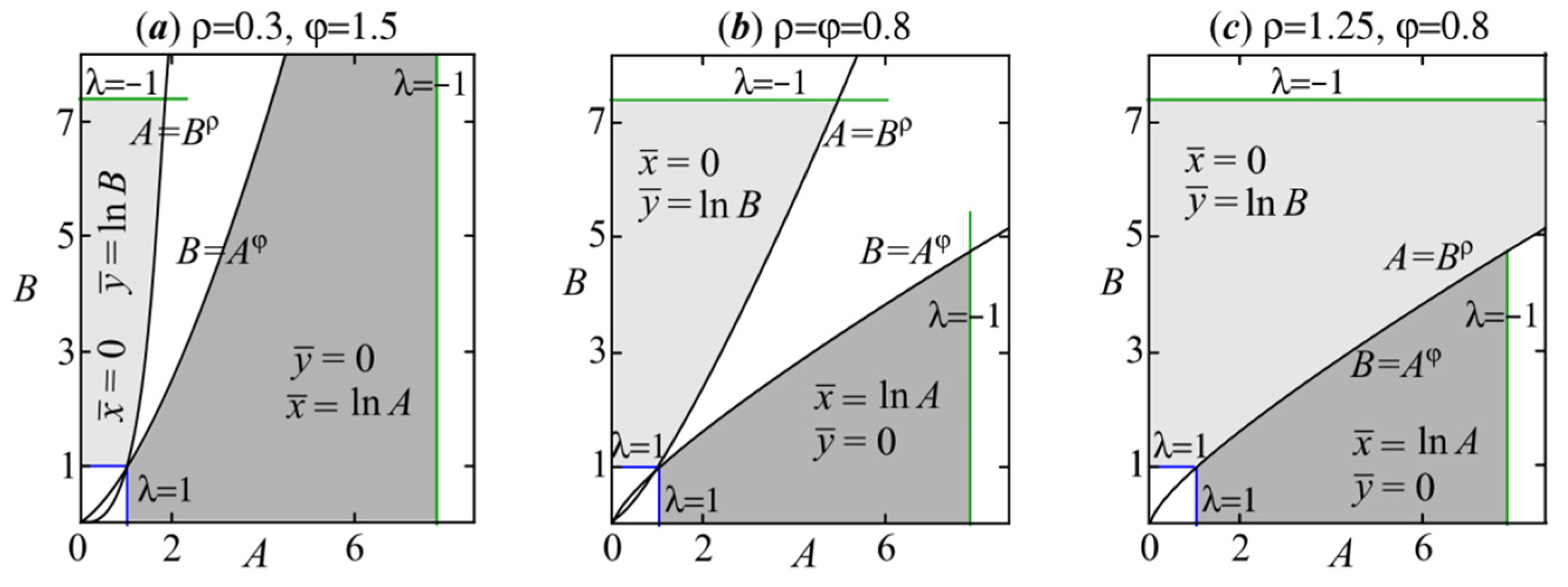
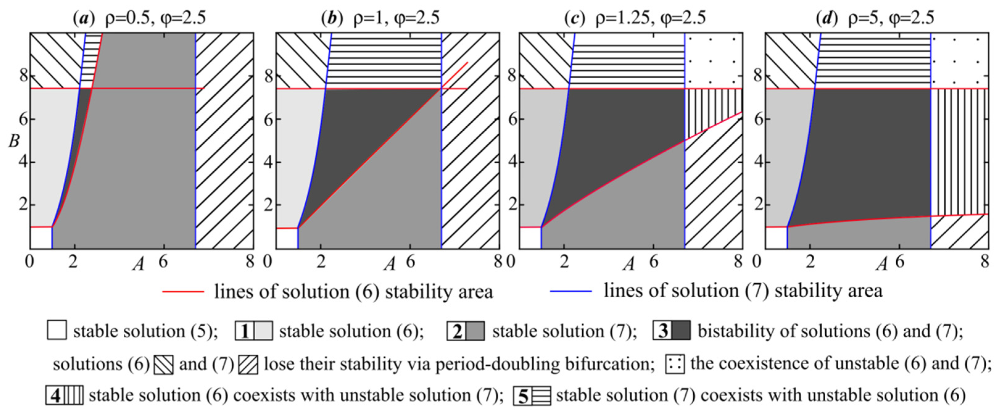
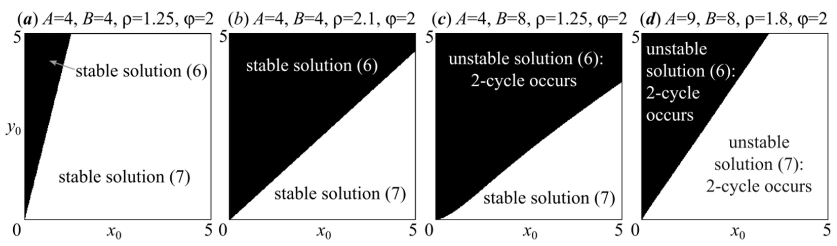
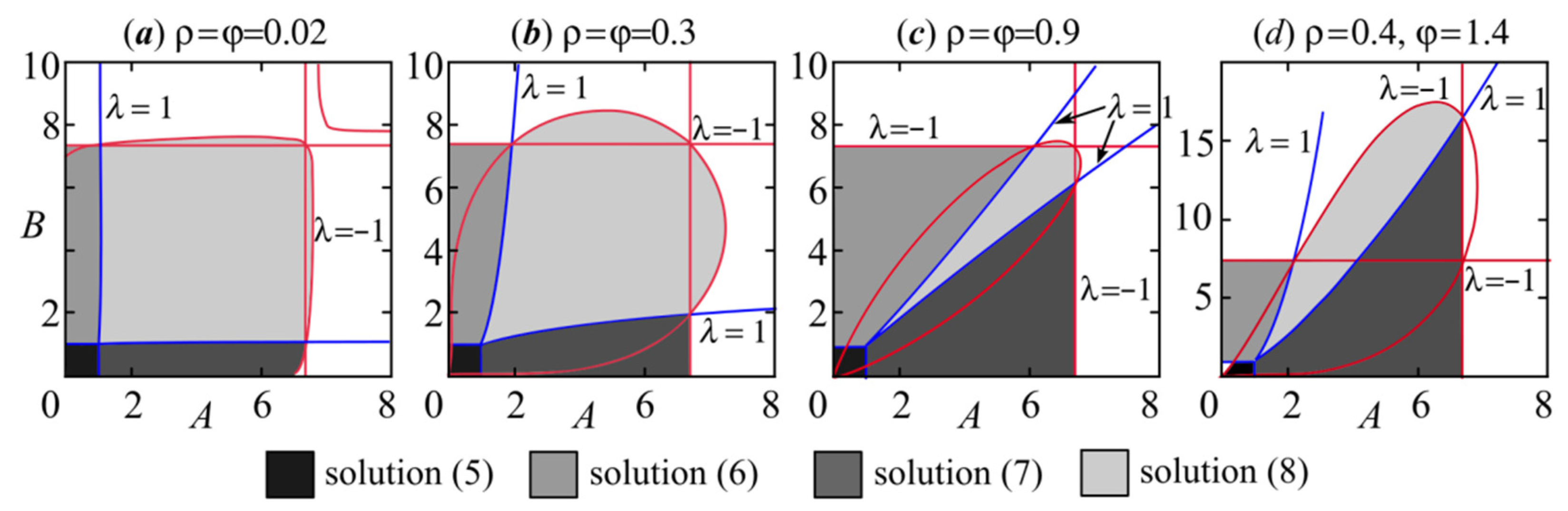
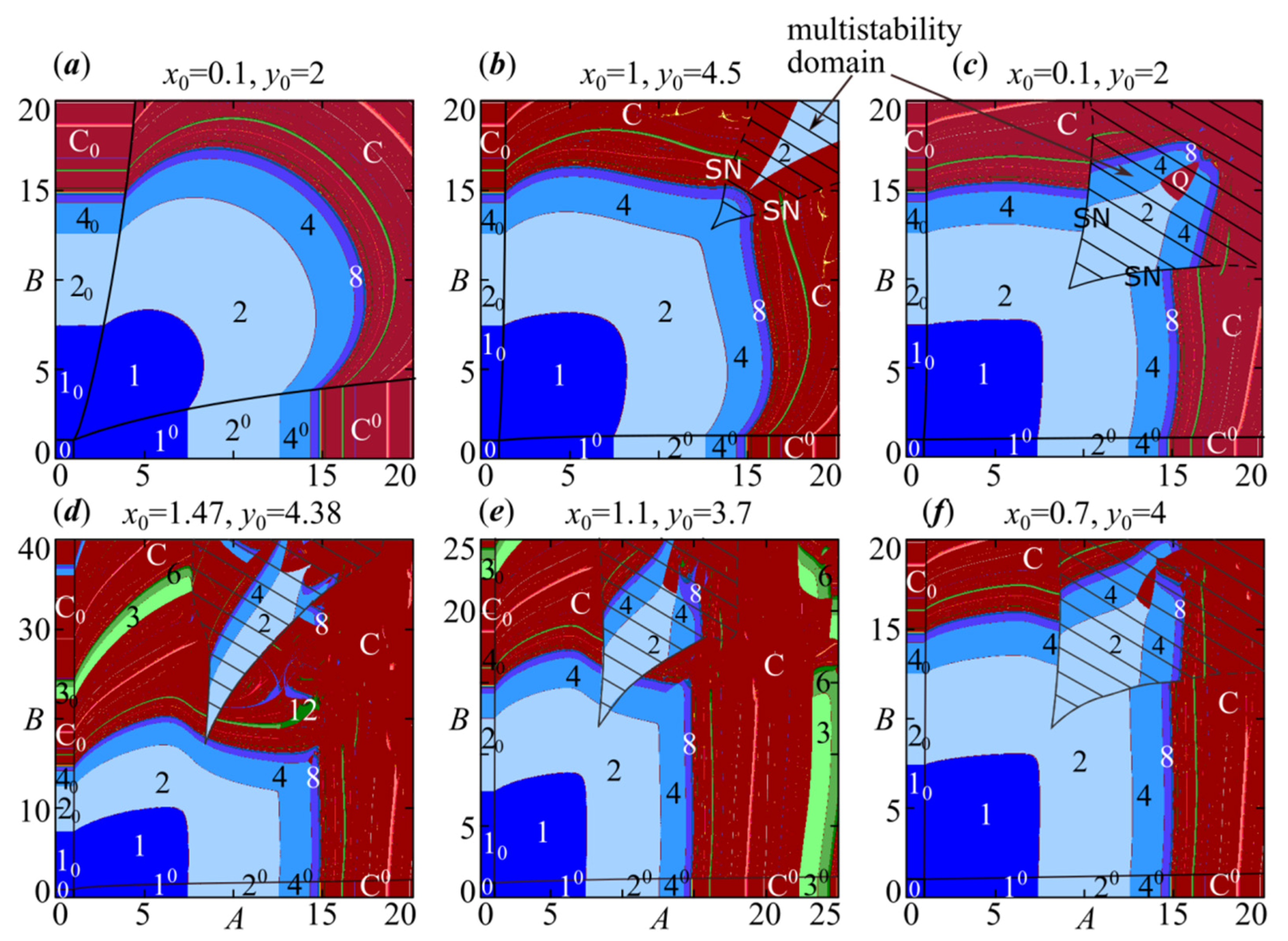
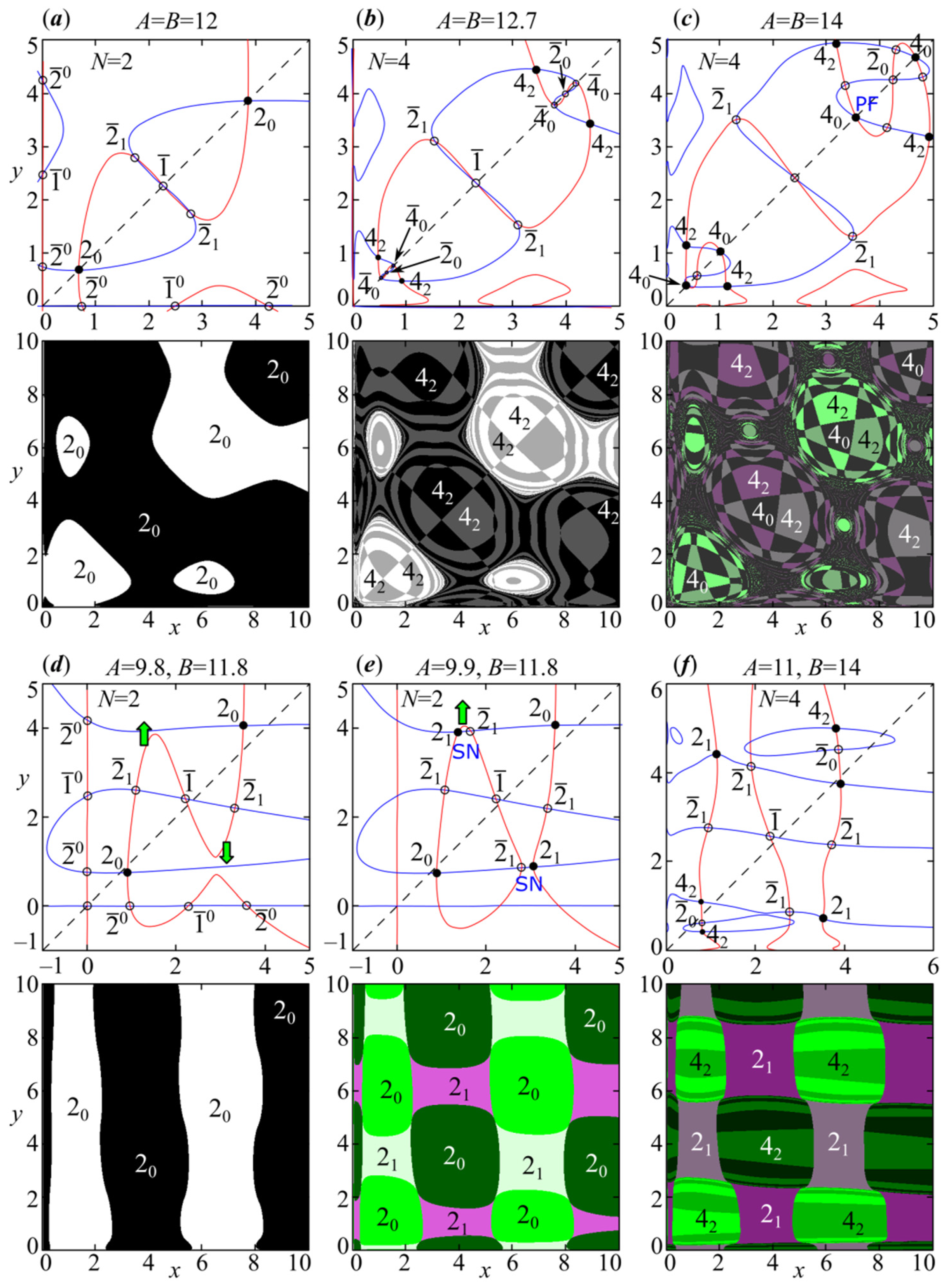
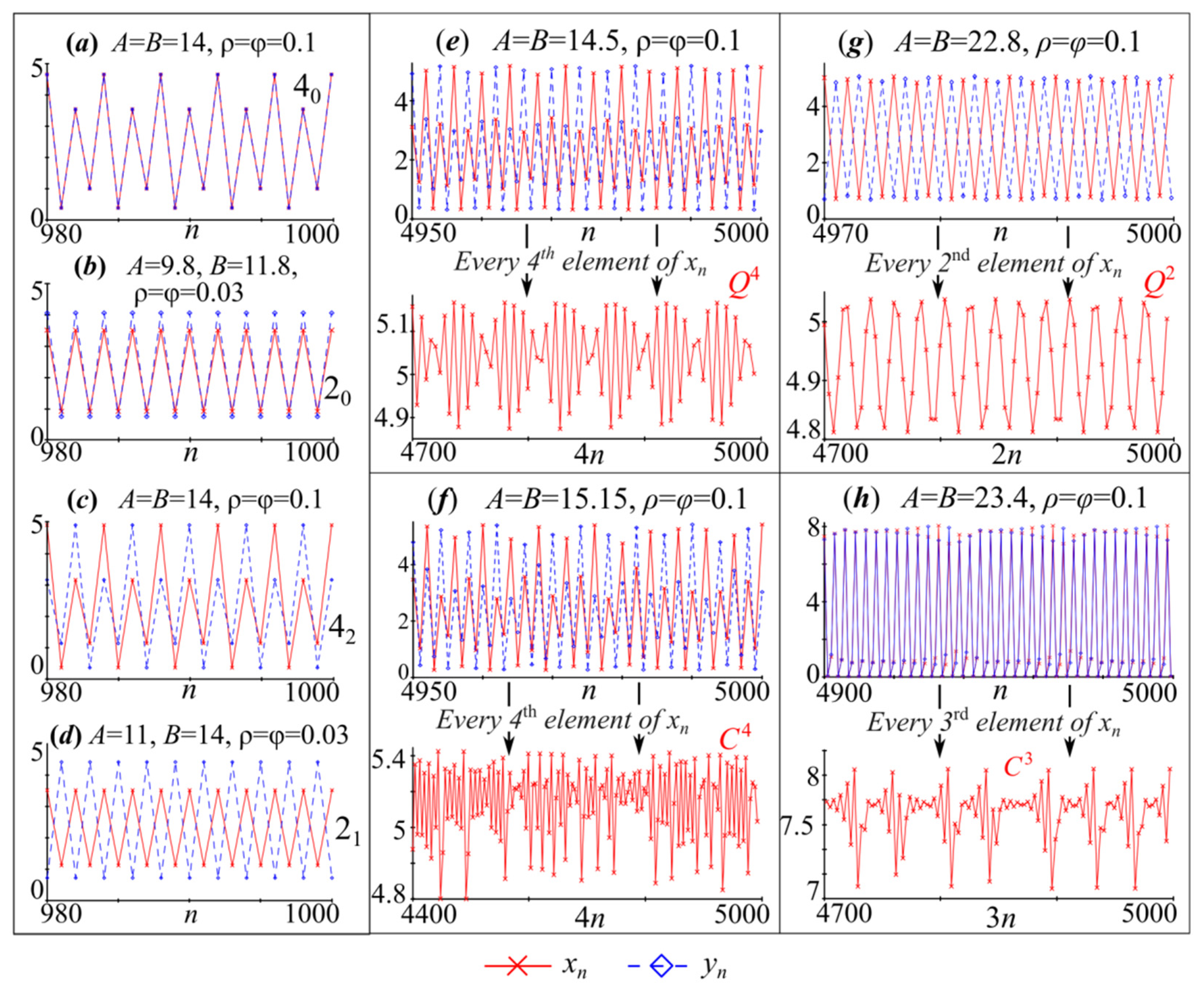
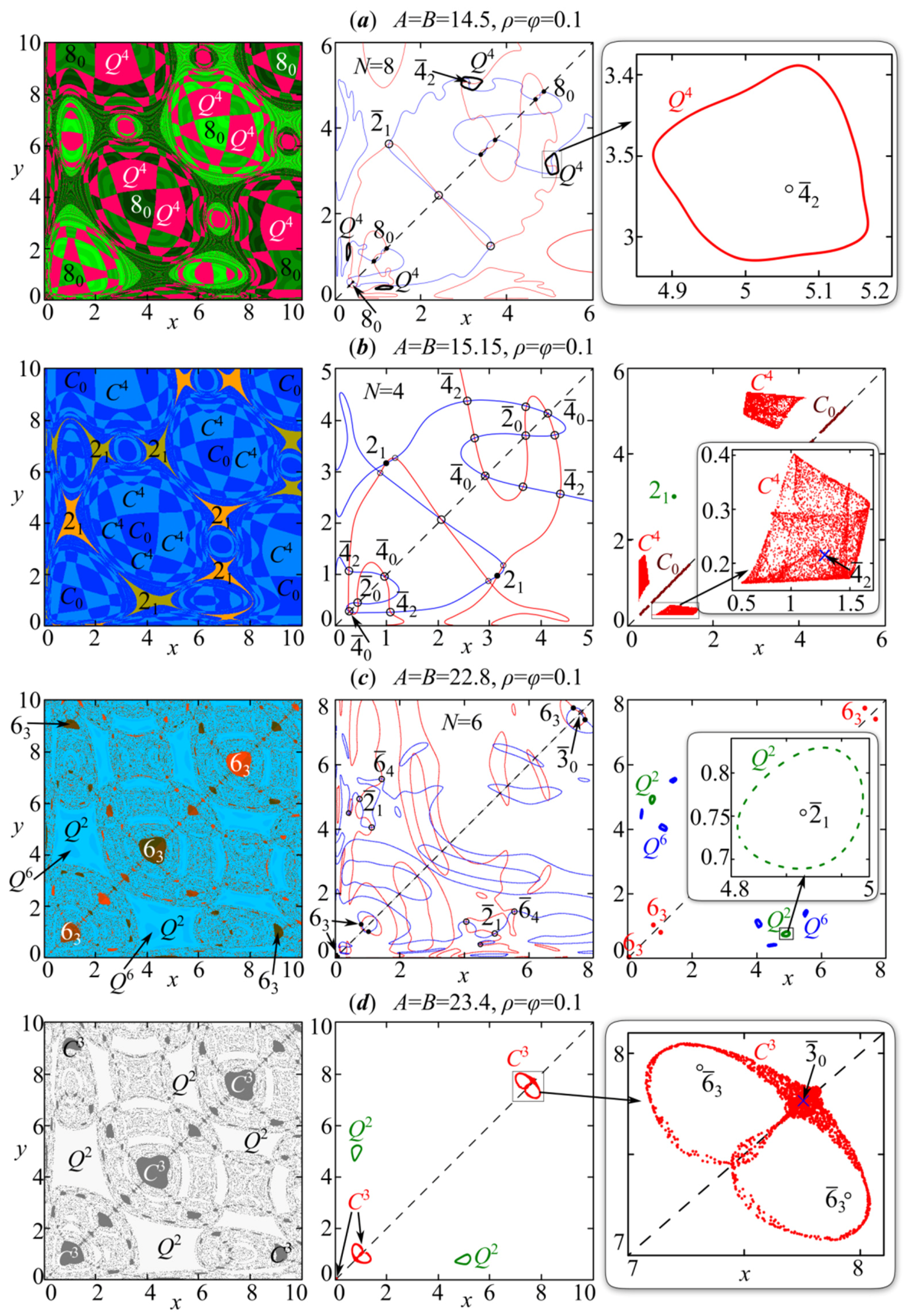
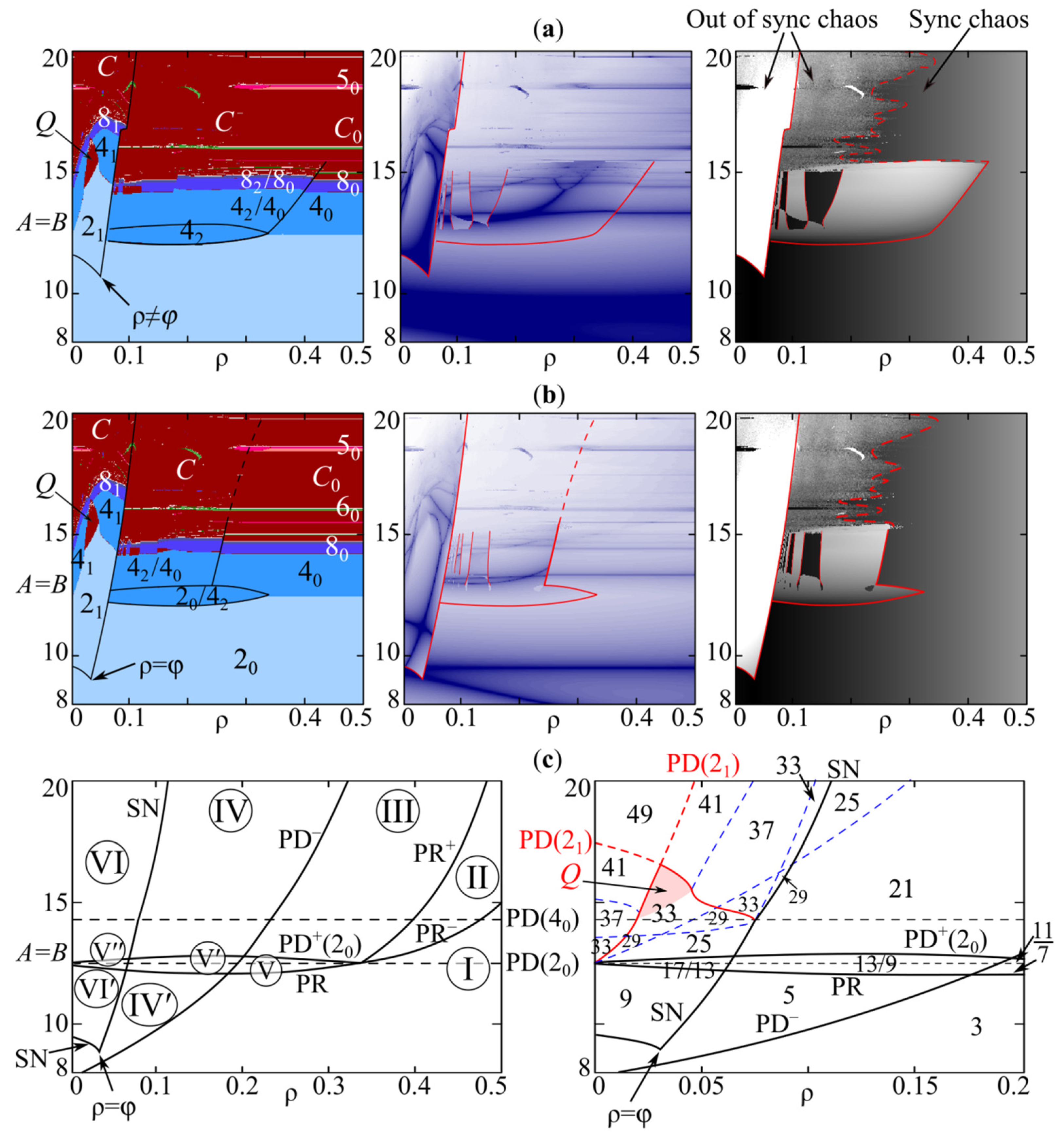
Table 1.
Development scenarios of competing populations depending on the parameter values.
| Intervals for the Parameter Values | Development Scenario | |
|---|---|---|
| species y displaces species x | ||
| species x displaces species y | ||
| species x and y coexist | ||
| species y displaces species x | ||
| species x displaces species y | ||
| the displacement of a species by another one depends on the values of initial conditions | ||
Publisher’s Note: MDPI stays neutral with regard to jurisdictional claims in published maps and institutional affiliations. |
© 2022 by the authors. Licensee MDPI, Basel, Switzerland. This article is an open access article distributed under the terms and conditions of the Creative Commons Attribution (CC BY) license (https://creativecommons.org/licenses/by/4.0/).
Share and Cite
MDPI and ACS Style
Kulakov, M.; Neverova, G.; Frisman, E. The Ricker Competition Model of Two Species: Dynamic Modes and Phase Multistability. Mathematics 2022, 10, 1076. https://doi.org/10.3390/math10071076
AMA Style
Kulakov M, Neverova G, Frisman E. The Ricker Competition Model of Two Species: Dynamic Modes and Phase Multistability. Mathematics. 2022; 10(7):1076. https://doi.org/10.3390/math10071076
Chicago/Turabian StyleKulakov, Matvey, Galina Neverova, and Efim Frisman. 2022. "The Ricker Competition Model of Two Species: Dynamic Modes and Phase Multistability" Mathematics 10, no. 7: 1076. https://doi.org/10.3390/math10071076
Note that from the first issue of 2016, this journal uses article numbers instead of page numbers. See further details here.