
Adaptive Fuzzy Neural Network Harmonic Control with a Super-Twisting Sliding Mode Approach


1
College of IoT Engineering, Hohai University, Changzhou 213022, China
2
College of Mechanical and Electrical Engineering, Hohai University, Changzhou 213022, China
3
Jiangsu Key Lab. of Power Transmission and Distribution Equipment Technology, Hohai University, Changzhou 213022, China
*
Author to whom correspondence should be addressed.
Mathematics 2022, 10(7), 1063; https://doi.org/10.3390/math10071063
Submission received: 5 February 2022
/
Revised: 23 March 2022
/
Accepted: 23 March 2022
/
Published: 25 March 2022
(This article belongs to the Special Issue Advances in Intelligent Control)
Abstract
:This paper designed an adaptive super-twisting sliding mode control (STSMC) scheme based on an output feedback fuzzy neural network (OFFNN) for an active power filter (APF), aiming at tracking compensation current quickly and precisely, and solving the harmonic current problem in the electrical grid. With the use of OFFNN approximator, the proposed controller has the characteristic of full regulation and high approximation accuracy, where the parameters of OFFNN can be adjusted to the optimal values adaptively, thereby increasing the versatility of the control method. Moreover, due to an added signal feedback loop, the controller can obtain more information to track the state variable faster and more correctly. Simulations studies are given to demonstrate the performance of the proposed controller in the harmonic suppression, and verify its better steady-state and dynamic performance.
1. Introduction
With the rapid development and application of distributed power generation, power electronic loads, AC and DC equipment, and electronic transformers, the electronic features in modern power grid are remarkable [1,2]. In the traditional power grid, the small number of harmonic sources and high concentration results in a harmonic level that can be controlled through the point-to-point management of users [3]. Now, however, the high-density access of a large number of electronic equipment makes the harmonic pollution of the grid difficult to handle, where the user-side point-to-point management model cannot meet the demand. Therefore, it is necessary to explore new methods to solve the harmonic problem of power electronic distribution network. Active power filters (APF) are widely used in improving power quality, where the compensation current control is a key technology [4,5,6,7,8].
Since APF is widely used in power systems, in recent years, many scholars have improved the efficiency of APF by applying advanced control methods [9,10,11]. As an unconventional, approximately continuous system with discontinuous properties, the exact physical model of APF system can be derived from the extensions and applications of Filippov theory in [12]. Nersesov and Haddad designed hybrid finite-time stabilizing controllers for impulsive dynamical systems, revealing the controllability and robustness against full modeling uncertainty [13]. Abdeslam et al. introduced a neural network method for extracting additional voltage components based on Adalines to recover a balanced voltage system in [14]. Wang et al. designed a one-cycle controlled DC side APF on the basis of analyzing its circuit topology and basic principle in [15]. Hua et al. shows the connection between the APF system and the Lyapunov method in [16]. Lam et al. proposed an adaptive thyristor-controlled LC-Hybrid APF to reduce switching loss in [17]. Wang et al. designed a model predictive control scheme combined with finite switching state characteristics in [18]. Lock et al. proposed a DSP-based one-cycle control strategy for a shunt active power filter in [19]. D’Abbico et al. used first-order ordinary differential equations as the approximate expression of the specific system, showing the excellent generality of ordinary differential equations in system modeling [20]. In the control of nonlinear systems, sliding mode control (SMC) has not only strong robust performance, but also high control accuracy. In order to efficiently control the position of the permanent magnet linear synchronous motor mover, an adaptive fuzzy fractional SMC strategy is proposed in [21]. An adaptive time-delay control scheme for mechanical system was proposed in [22]. Hou et al. developed a feedback sliding mode control architecture in the presence of modelling system uncertainties [23]. Singh et al. proposed a recursive backstepping sliding mode control which has a good effect on the control of parameter disturbance [24]. The practical tracking control design of robot manipulators with continuous fractional-order nonsingular terminal sliding mode based on time-delay estimation was studied in [25], which requires no detailed information about the robot dynamics.
However, chattering is a serious problem in sliding mode control. As a high-level SMC algorithm, a super-twisting SMC (STSMC) algorithm can effectively reduce the chattering problem and make the control input smoother. The precise analytical expression for the finite arriving time of the super-twisting algorithm without disturbances was derived, and a new estimation algorithm for the upper bound of the arrival time with disturbances was proposed in [26]. A super-twisting sliding mode control for a wind energy conversion optimization problem was studied in [27]. A super-twisting method to build an output feedback stabilization strategy was developed for a perturbed double-integrator system in [28]. A direct super-twisting control power control method was investigated to control a brushless doubly fed induction generator in [29].
A neural network method is an effective way to deal with the model uncertainty in APF. An adaptive nonlinear disturbance observer with a wavelet neural network was studied in [30]. The neural network method is widely used in the control of various dynamic systems combined with sliding mode control. A hybrid control method based on RBF neural network and super-twisting sliding mode control was proposed for a micro gyroscope in [31], where a neural network is used to improve the stability and performance of the system. Hayakawa et al. proposed a hybrid adaptive control framework based on a neural network for nonlinear uncertain dynamical systems, which guarantees partial asymptotic stability basing on the Lyapunov stability theory [32]. El-Sousy proposed an adaptive dynamic sliding mode control system with an output feedback radial basis function (RBF) network for an indirect field oriented control induction motor drive in [33].
Due to the poor dynamic characteristics of the traditional one-way neural network, the output feedback neural network (FNN) composed of the feedback loop which can obtain more dynamic information came into being. For example, traditional RBF network requires high quality of parameters, which relies on trial and experience of the designer. However, owing to the superior learning ability, FNNs have the adaptive ability of adjusting parameters with higher efficiency, which can be supported by a novel recurrent neural network controller in [34]. Moreover, for ordinary neural networks with a single hidden layer, it is difficult to estimate some fairly complex functions with high accuracy. To solve the problem, traditional way is to lengthen the sensing area or raise the number of neurons, but they will lead to long training time or high memory consumption. Therefore, in order to obtain fast learning speed and high learning accuracy, a deep neural network with multi-layer is necessary. Advanced intelligent control schemes with multi-layer neural network have been developed for dynamic systems [35,36,37,38].
Motivated by the above-mentioned works, this paper proposes an adaptive super-twisting sliding mode (STSMC) control method for active power filter based on an output feedback fuzzy neural network (OFFNN). The advantages of the proposed methodology with respect to previously published results are explained in the following procedures. The adaptive super-twisting sliding mode controller has not been applied to the harmonic suppression of active power filter before. It can deal with high-frequency dynamics and reduce the chattering. An output feedback fuzzy neural network with two hidden layer and internal and external feedbacks can fit more complex functions, and improve training accuracy through fast convergence.
(1) As a high-order sliding mode controller, the adaptive super-twisting sliding mode control is used to reduce the chattering. It guarantees strong robustness while possessing better smoothness, so the high-frequency dynamics problem can be dealt with. It requires less information and reduces the requirements of modeling accuracy, thereby simplifying the complexity of the algorithm.
(2) An output feedback fuzzy neural network is used to estimate uncertainty, including both unknown system characteristics and external disturbance. It has the characteristics of two hidden layer and internal and external feedbacks, therefore it is suitable to be used for the approximation. In order to make up for the gap between local optimization characteristics of traditional fuzzy neural network and wide range of changes of APF signals, internal and external feedbacks are used to increase the information of the neural network, thereby giving the neural network a wider range of learning and making the network more powerful to learn complex things.
(3) The OFFNN can set the initial values of the parameters such as center vectors and the base widths arbitrarily, which can be adaptively adjusted to the optimal values, according to the adaptive algorithm. It makes the neural network less reliant on human experience, thereby raising the universality of the control method.
(4) Since the control methods used in this paper use generalized models, the control method is of great universality, and can deal with more kinds of uncertainties and disturbance compared with traditional resonant controllers, which needs the model to be as exact as possible. Moreover, the entire control strategy can ensure the stability of the system while improving the total harmonic distortion performance.
The rest of this paper is organized as follows. In Section 2, the proposed OFFNN is introduced, along with detail about its structure and working principle. In Section 3, a dynamic mathematical model of APF is established. Section 4 introduces the whole structure, designing process, and stability analysis of proposed STSMC-OFFNN method. The simulation experiment is described in Section 5. Section 6 draws the paper to a conclusion.
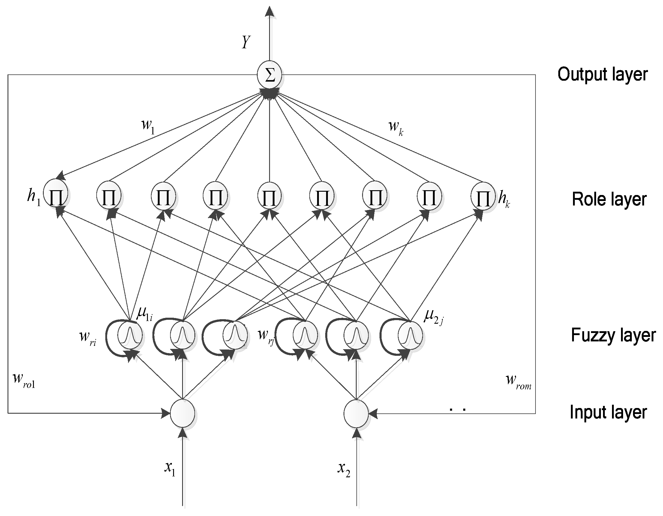
2. Output Feedback Fuzzy Neural Network Structure
The OFFNN has both an internal feedback network and an external feedback network, collecting internal state information and external output information at the same time. The main advantage of the OFFNN is that the initial values of its center vector and base width can be set arbitrarily, and the optimal value can be achieved through online adjustment efficiently.
The structure of the OFFNN is a four-layer neural network with two layers of feedback, as shown in Figure 1. The function of each layer is introduced as:
(1) Input layer: its main function is to accept the network input and the network output in the previous loop, then pass it to the next layer. The input layer and the output layers are connected by the weights of the outer feedback fuzzy neural network , and the output signal of the input layer is . is expressed as:
(2) Fuzzy layer: its main function is to calculate the membership function, where the Gaussian function is selected. This layer can adaptively adjust the membership through the feedback information of the network output, so as to reduce the influence of initial value. This layer’s feedback fuzzy neural network weights are calculated with the Gaussian function, using the weights’ values of the previous round and the input signal transmitted from the input layer. Suppose the output of this layer is ... (), there are:
where are the internal feedback gains, is the center vector, and is the base width.
(3) Rule layer: this layer mainly multiplies the weights of membership with the input and sends it to the output layer. The output of the rule layer is:
where .
(4) Output layer: the main function is to integrate the output of the rule layer and obtain the final network output. The output layer neuron is connected with the rule layer through the weight , and the signal node of the output layer is marked as , meaning the sum of all input signals, as follows:
where , .
In addition, the output layer neuron feeds it back to the input layer and the fuzzy layer. It connects with the input layer neuron through the weight of outer layer feedback.
3. Modeling of Active Power Filter
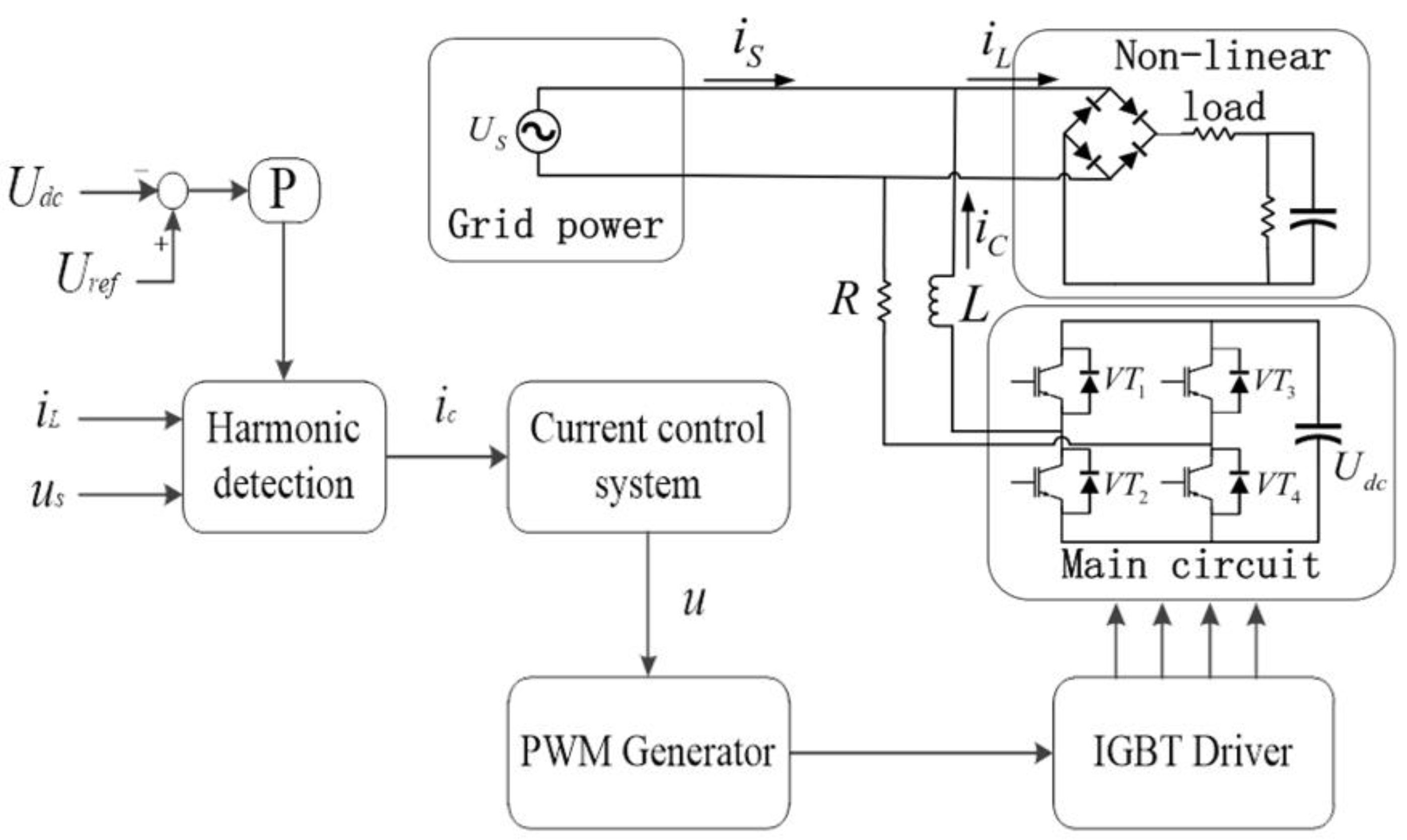
A typical single-phase APF mainly includes three parts: grid voltage, non-linear load, and main circuit. In this paper, the main circuit of the APF is regarded as an inverter circuit which can be controlled by PWM trigger pulses. IGBTs are selected as switching devices. To achieve stable voltage, a DC-side capacitor is used as the source. A single-phase uncontrollable rectifier bridge with capacitive load is used as a nonlinear load. The main structure is as shown in Figure 2.
Setting the grid power and main circuit as a voltage loop, according to Kirchhoff’s voltage theory, it is obtained as:
where us is a grid voltage, ic is a compensation current, udc is a DC side capacitor voltage, and L and R are the inductance and resistance of the active filter main circuit, respectively. Q is the switch function. Then, we define the switch function Q as follows:
In the DC-side voltage, the sheer proportional control method can achieve the voltage stability requirements easily, so the main subject is the state equation of the compensation current, derived as:
Generally, for the needs of higher-order controller design, in power electronics modeling, the active power filter system model is usually considered as a second-order model. Therefore, taking the derivative of Equation (8) produces:
Considering the expression of Q, it is concluded that the is 0 most of the time. When it comes to the switching point, although the has an extreme large absolute value, its duration is too short to influence the system due to the filter characteristic of L in Figure 2, so the is often ignored. Then, Equation (9) can be rewritten as follows:
where q represents ic, f(x) represents , B represents , and which is treated as a continuous function. When outputted to the IGBT, the continuous u should be transformed into PWM wave in PWM generator. This method slightly reduces performance and results in inevitable chattering, but allows for greater versatility and integration into existing physical systems.
Remark 1.
udc is far from rated value before charging, so ic in this period needs to compensate iL and to raise udc. With the finish of charging, the error greatly reduces, so the duty to raise udc reduces its weight, and ic focuses on the compensation of iL.
Since the proposed control method focuses on harmonic compensation in a steady state, udc is set as a constant. The influence brought by error can be integrated in as in Equation (10), so it will not have great effect on the system. For the same reason, integral surface used on udc to keep it perfectly stable is also unnecessary.
In practical applications, considering the system uncertainty and external disturbance, the state equation of the compensation current is rewritten as:
where represents the lumped uncertainty.
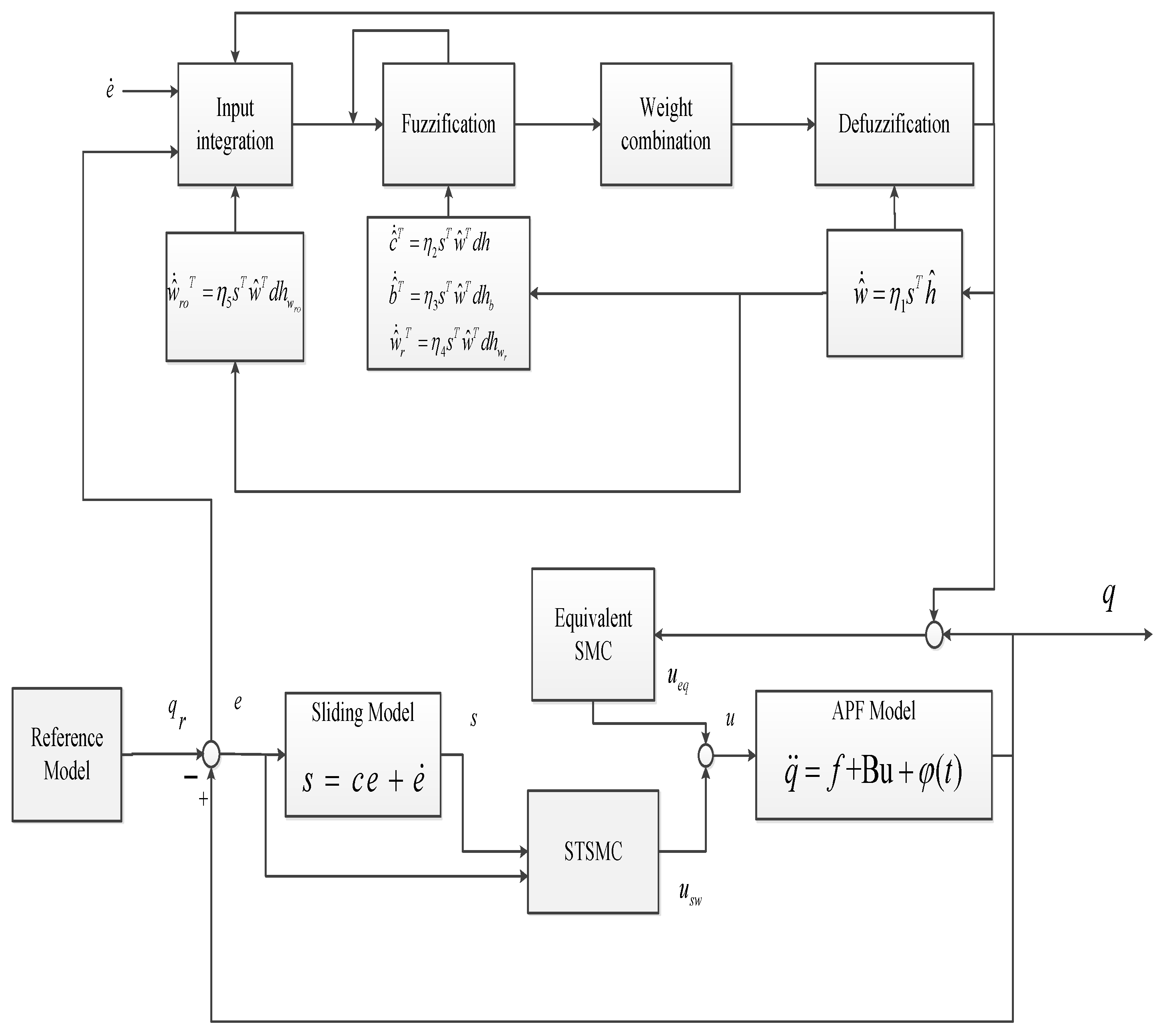
4. STSMC-OFFNN Controller and Stability Analysis
The OFFNN provides a solution to the uncertainties of actual system. It calculates a nearly approximate model of the system through adaptive approximation, so that the design of the controller does not need to rely on the exact model of the actual system. Furthermore, the parameters such as center vector, base width value, network weight, and feedback gain of the inner and outer loops of OFFNN can be fully adjusted according to the adaptive laws. In this way, the approximation accuracy of the neural network can be improved, and the dependence of the neural network on parameters can be reduced, improving the availability of controller output.
The sliding surface is designed as:
where is the coefficient of the sliding mode surface, are tracking error and the derivative of the tracking error, respectively, and can be expressed as:
and
Then, the derivative of sliding mode surface is expressed as:
Substituting Equation (11) into Equation (15) yields:
Ignoring the model uncertainty and external disturbance, setting , the equivalent control law is obtained as:
Based on the STSMC algorithm, the switch control law is designed as:
where , and , where and are the upper bound of the system uncertainties and external disturbance and its derivative, respectively.
Then, the controller is designed as:
The OFFNN is used to approximate the unknown model part of the system, and the approximation function of the is expressed as , so the control law Equation (19) is revised as:
where is used to ensure the consistency of the form with the neural networks.
Use * as the symbol for the optimal value. Assuming there are best weight , base width , center vector , inner feedback gain , and outer feedback gain , use to estimate . Taking the errors caused by different data structures into consideration, there is:
where , and is mapping errors.
Define the superscript ~ as the symbol of error between ideal value and actual value. Define the error of each parameter in the approximation model as:
Therefore, the error between the unknown model and the approximation model can be expressed as:
Define the total approximation error as:
Thus, Equation (23) can be derived as:
In order to realize the online adaptive adjustment of the parameters of OFFNN approximator, the Taylor expansion is performed on , obtaining the following expression:
where is high-order terms. The coefficient matrices are denoted as
Substituting Equation (26) into Equation (25) yields:
Define the sum of approximation errors as: . Assume that it and its detective are bounded, and satisfy the condition , where is a positive constant.
To achieve good tracking effect of , adaptive laws are designed as:
where η1, η2, η3, η4, η5 are positive constants.
The control structure diagram of the system is shown in Figure 3.
The Lyapunov function candidate is selected as follows:
Define:
Then, the derivative of Equation (32) can be obtained as:
Substituting Equations (16) and (20) into Equation (32) yields:
Substituting Equation (28) into Equation (33) yields:
Substituting Equation (29) into Equation (34) yields:
Since , Equation (35) can be simplified as:
Therefore, if inequality below can be proved:
Thus:
Since V(0) is bounded and V(t) is also bounded because and , it is obtained that is bounded. With the condition that is bounded and Barbalat’s lemma, s(t) will asymptotically converge to zero. Thus, the designed controller can guarantee the asymptotic stability of the closed-loop control system.
5. Simulation Study
In order to prove the feasibility and effectiveness of the above-mentioned adaptive super-twist sliding mode control based on OFFNN, a simulation experiment is carried on the MATLAB/SIMULINK. The system’s main parameters are selected as in Table 1. To show the adaptive ability of OFFNN, the initial values of b, c, w, and wr, are all set as 1, wro is set as 0. The values η1, η2, η3, η4, and η5 are set as 5 × 10⁸, 1 × 10⁸, 1 × 10⁸, 1 × 10⁸, and 1 × 10⁹. The values k1, k2 are set as 2 and 3.
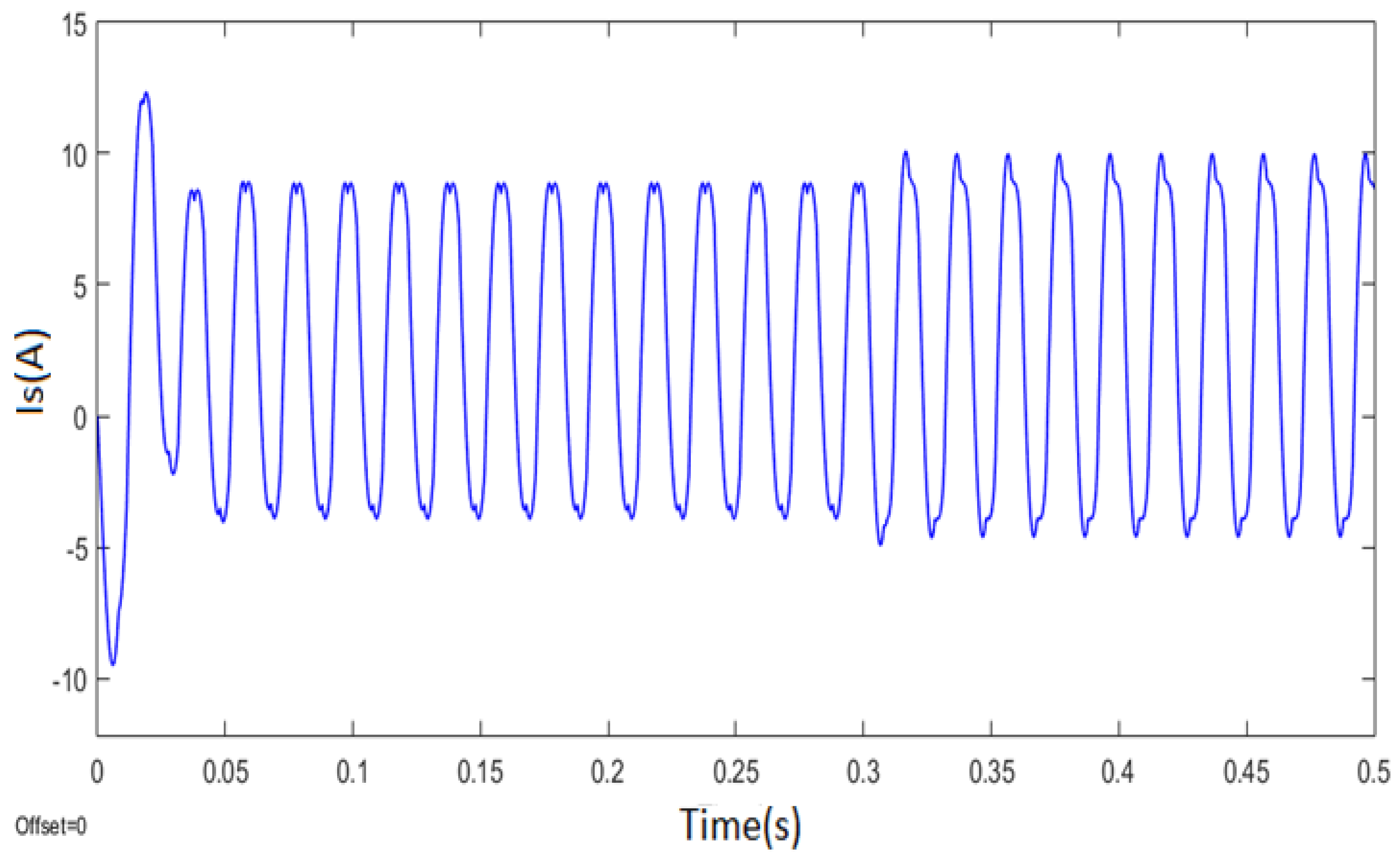
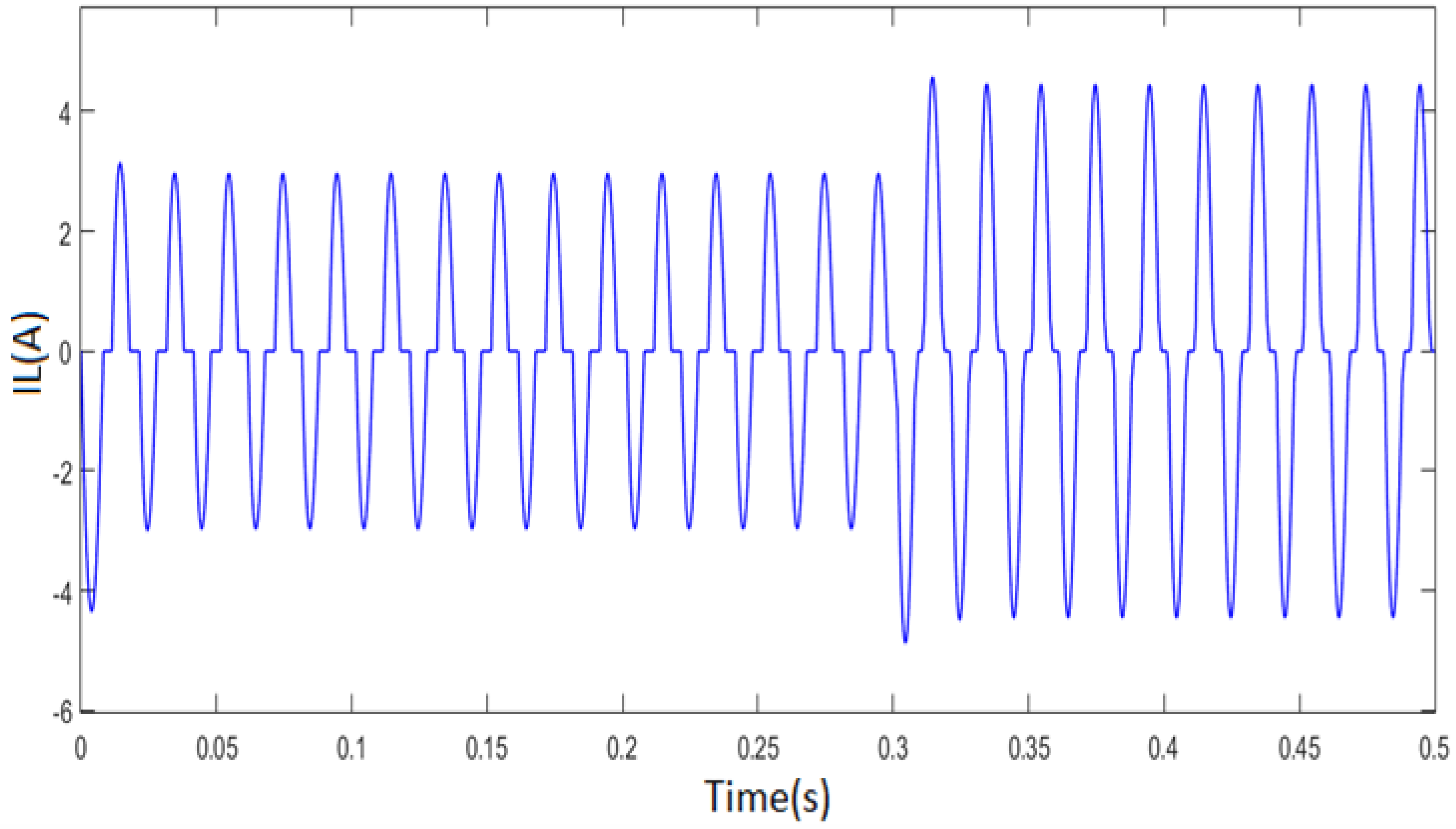
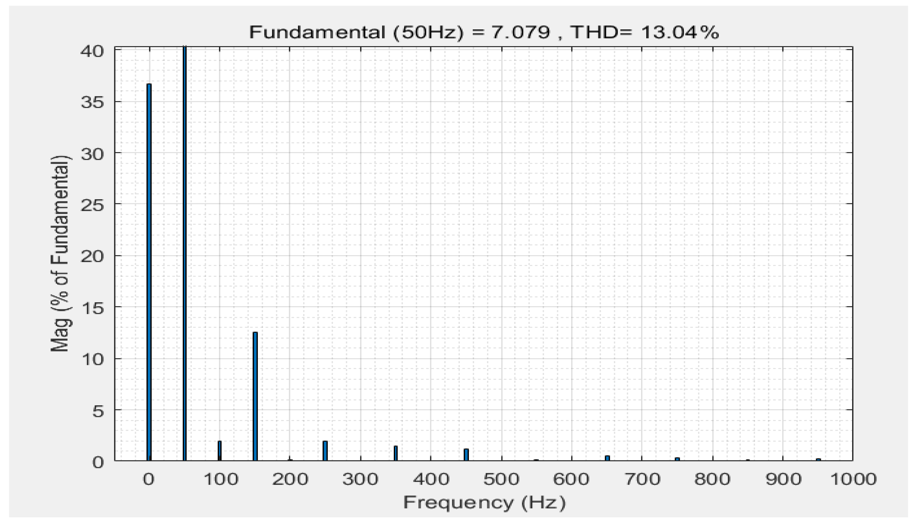
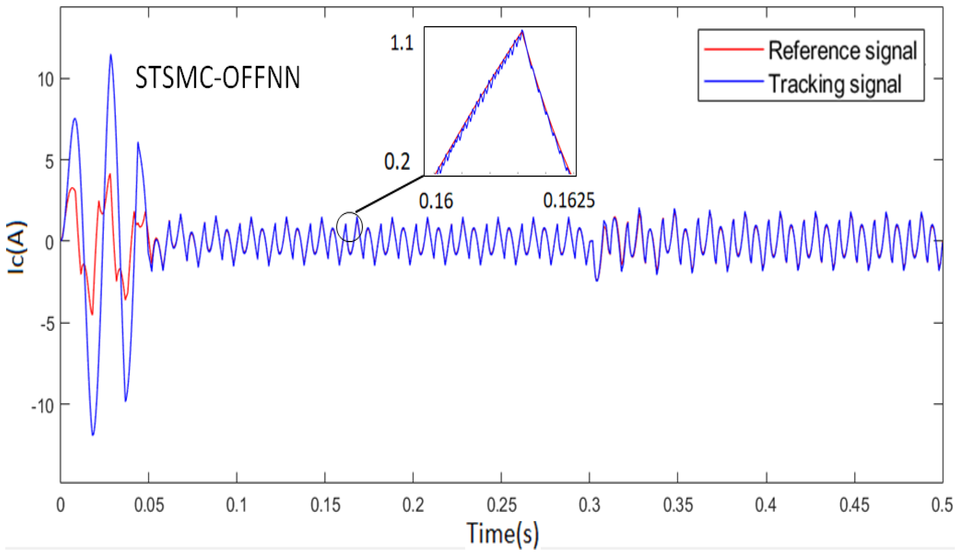
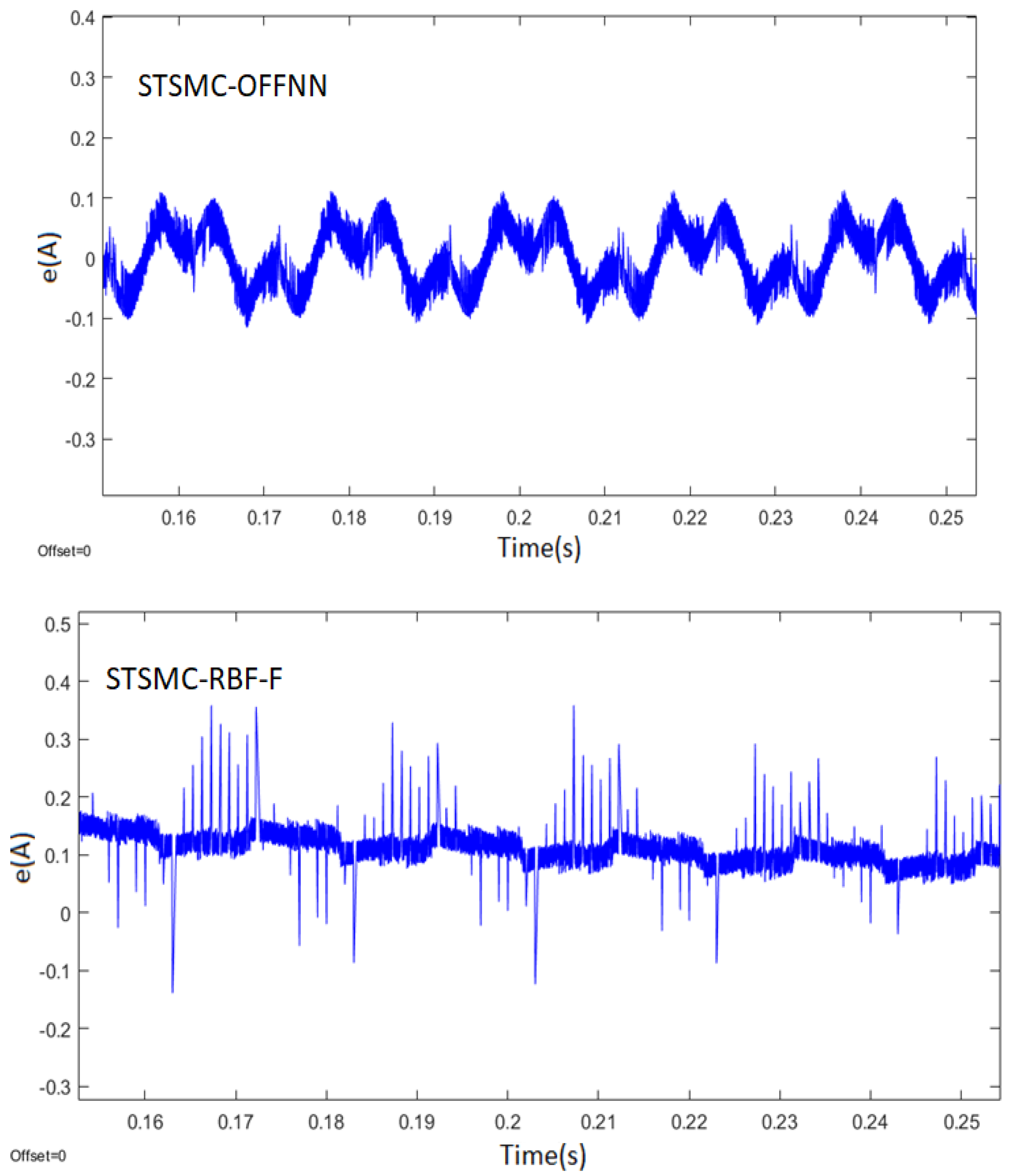
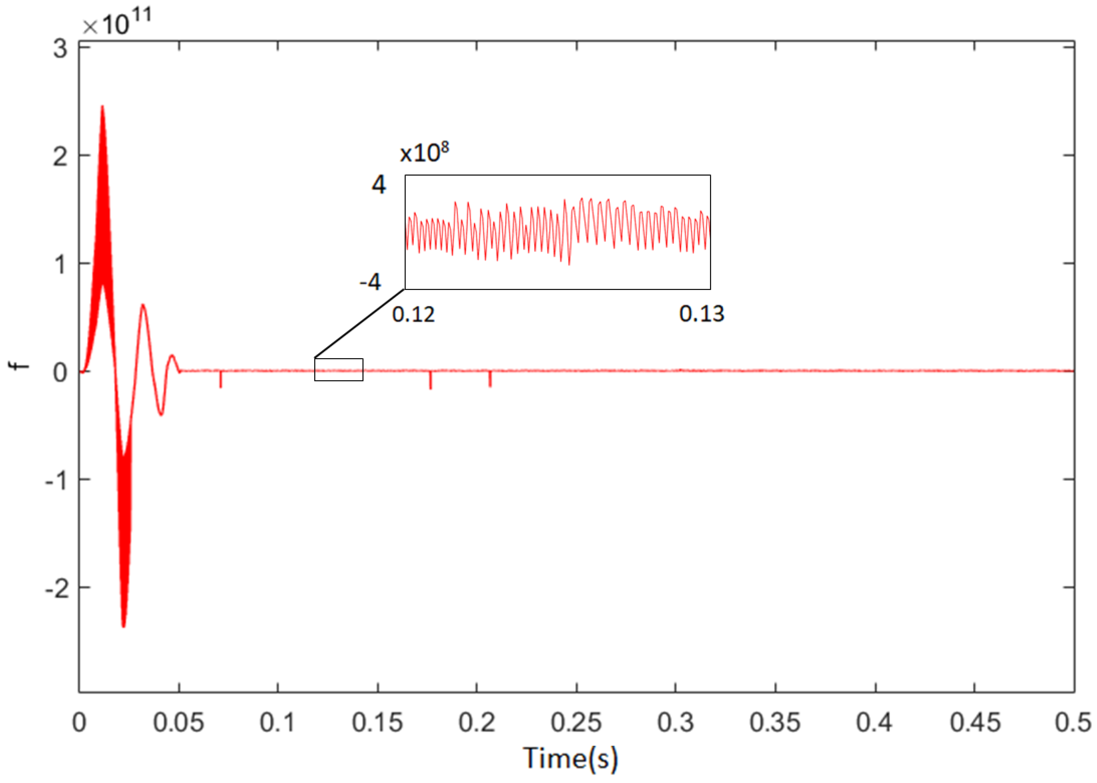
Figure 4 and Figure 5 give the simulation results without any controller. The load is turned on in 0.3 s. It can be seen that, due to the distortion of load current, the power supply current has some distortion at both peaks, preventing it from performing as a perfect sine wave. In APF, total harmonic distortion (THD) is often used to evaluate the performance of the system. Its THD is shown in Figure 6, which is up to 13.04% further from the satisfactory value. Figure 7 and Figure 8 are the performance of the proposed STSMC-OFFNN and its comparison with two other control systems, including STSMC and STSMC-RBF-F. In STSMC-RBF-F, the last F stands for the additional filter, since RBF itself is hard to deal with when implemented in such a fast-changing object. From Figure 7, it is clear that STSMC does not have the ability to complete the control requirement, showing the necessity of incorporating additional parts to the control method. It can be seen in Figure 8 that the STSMC-OFFNN is superior to the comparison method in terms of system performance to STSMC-RBF-F, proving that the compensation current can track the command current well, as well as verifying the excellent stability and robustness of STSMC-OFFNN. Moreover, the fact that the output is smoother, namely the chattering is smaller, indicates the internal soft changes of the system. The THD data in Table 2 indicate that STSMC-OFFNN has a good effect in eliminating harmonics and can effectively purify harmonic pollution.
Remark 2.
In Figure 7, the reference signal of the STSMC method differs from others because the reference signal is affected by system status. Thus, with the inadequate control of STSMC method, the reference signal is influenced.
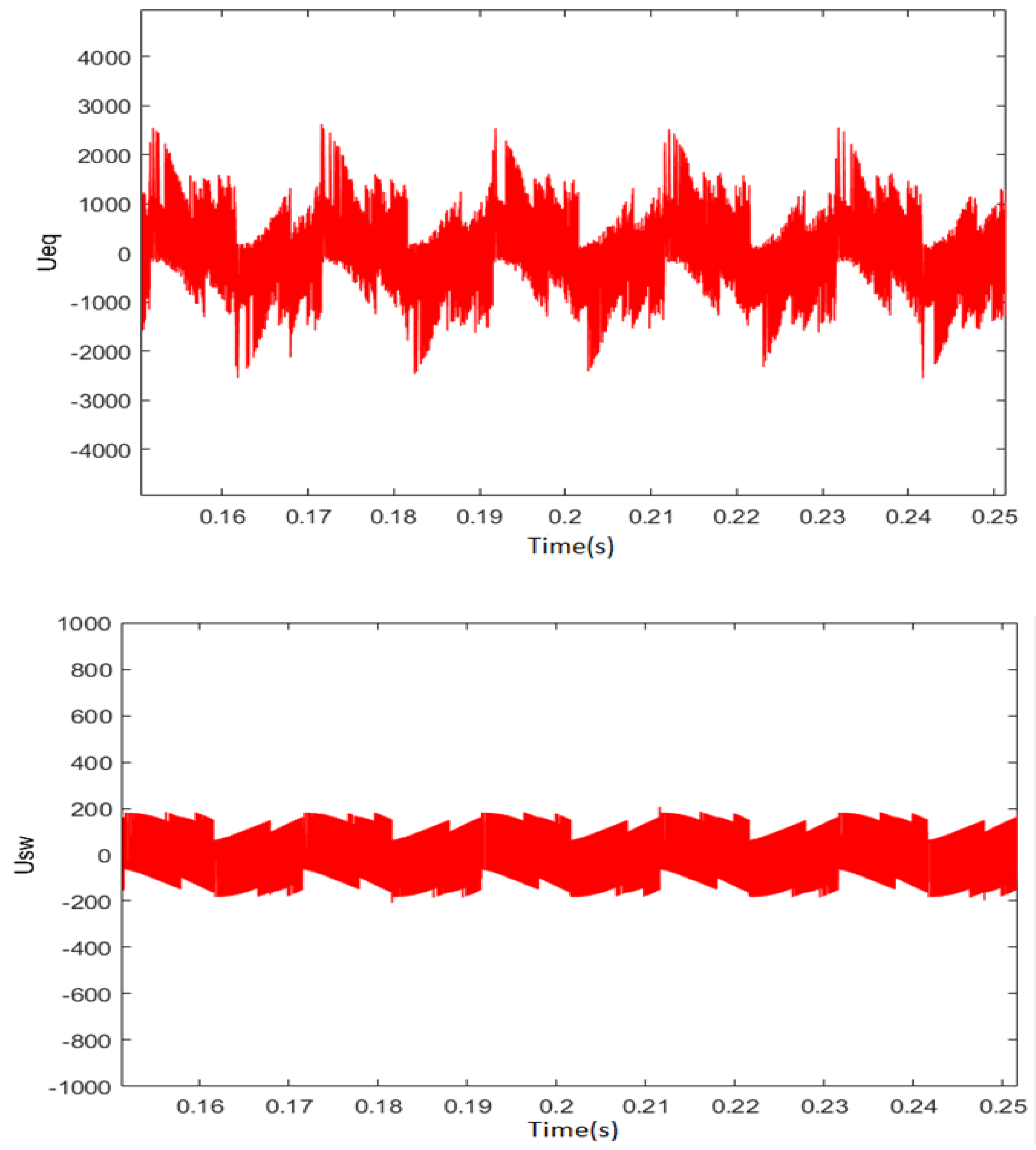
Figure 9 is the comparison of ueq and usw, showing that ueq has higher magnitude of output, and also demonstrating that OFFNN dominates the control process and STSMC has an accessorial compensation in the control method. Due to the structural characteristics of APF Systems, the chattering problem is hard to completely resolve, but compared with the traditional switching control law, STSMC has the effect of reducing jitter amplitude.
Figure 10 is the adaptive curve of the OFFNN, showing that the output of the OFFNN does not require manual adjustment, and can quickly self-converge through an adaptive method, so that the system can obtain the optimal neural network performance to reach the optimal output. This shows that this neural network has good stability and self-regulation ability. The high initial value results from a high study rate of OFFNN. Considering its proportion in the whole process, the influence is limited.
Table 3 shows the further performance comparisons of the STSMC-OFFNN and STSMC-RBF-F. It can be seen that the variation of the load has little effect on the performance of the system, and the proposed STSMC-OFFNN method can achieve a better control effect than the traditional method in all cases shown. It is also shown that capacitive load will not have bad influence on the performance. All of these prove the superiority of the proposed method.
6. Conclusions
In this paper, an adaptive super-twisted sliding mode control method based on a novel fuzzy neural network is proposed to solve the problem of harmonic pollution in APF systems. An output feedback fuzzy neural network is designed to increase the accuracy and performance of the neural network. Its characteristic of two hidden layer helps to maintain good balance on approximation speed and accuracy. Furthermore, feedbacks are used to broaden the learning scope of neural networks, therefore better handling of wide-amplitude, fast-changing signals. Compared with traditional proportional-integral or proportional-resonant methods, the proposed control method has the advantage of low model and parameter dependencies owing to its adaptive learning ability. Thanks to this, when dealing with complex and changeable systems or systems with immeasurable parameters, the proposed method has stable and reliable control performance. Compared with the traditional neural network method, the improved structure of OFFNN is superior for its higher approximating speed and accuracy and its better compatibility with IGBTs. Simulation experiments verified that the proposed STSMC-OFFNN method can achieve satisfactory harmonic compensation performance in harmonic compensation, regardless of the system uncertainties and load variations. The comparison with traditional LCL and LLCL methods shows that the proposed general method has control performance comparable to that of the specialized method.
Author Contributions
Conceptualization, J.F.; methodology, Q.P., X.L.; writing—original draft preparation, Q.P.; writing—review and editing, J.F. All authors have read and agreed to the published version of the manuscript.
Funding
This work is partially supported by the National Science Foundation of China under Grant No. 61873085.
Conflicts of Interest
The authors declare no conflict of interest.
References
- Chauhan, S.K.; Shah, M.C.; Tiwari, R.R.; Tekwani, P.N. Analysis, design and digital implementation of a shunt active power filter with different schemes of reference current generation. IET Power Electron. 2014, 7, 627–639. [Google Scholar] [CrossRef]
- Panigrahi, R.; Subudhi, B.; Panda, P.C. Model predictive-based shunt active power filter with a new reference current estimation strategy. IET Power Electron. 2015, 8, 221–233. [Google Scholar] [CrossRef]
- Gomez Jorge, S.; Busada, C.A.; Solsona, J. Reduced order generalised integrator-based current controller applied to shunt active power filters. IET Power Electron. 2014, 7, 1083–1091. [Google Scholar] [CrossRef]
- Cao, D.; Fei, J. Adaptive Fractional Fuzzy Sliding Mode Control for Three-Phase Active Power Filter. IEEE Access 2016, 4, 6645–6651. [Google Scholar] [CrossRef]
- Biricik, S.; Redif, S.; Özerdem, O.C.; Khadem, S.K.; Basu, M. Real-time control of shunt active power filter under distorted grid voltage and unbalanced load condition using self-tuning filter. IET Power Electron. 2014, 7, 1895–1905. [Google Scholar] [CrossRef] [Green Version]
- Lei, D.; Wang, T.; Cao, D.; Fei, J. Adaptive Dynamic Surface Control of MEMS Gyroscope Sensor Using Fuzzy Compensator. IEEE Access 2016, 4, 4148–4154. [Google Scholar] [CrossRef]
- Yi, H.; Zhuo, F.; Zhang, Y.; Li, Y.; Zhan, W.; Chen, W.; Liu, J. A Source-Current-Detected Shunt Active Power Filter Control Scheme Based on Vector Resonant Controller. IEEE Trans. Ind. Appl. 2014, 50, 1953–1965. [Google Scholar] [CrossRef]
- Lascu, C.; Asiminoaei, L.; Boldea, I.; Blaabjerg, F. High Performance Current Controller for Selective Harmonic Compensation in Active Power Filters. IEEE Trans. Power Electron. 2007, 22, 1826–1835. [Google Scholar] [CrossRef]
- Hou, S.; Fei, J. A Self-Organizing Global Sliding Mode Control and Its Application to Active Power Filter. IEEE Trans. Power Electron. 2020, 35, 7640–7652. [Google Scholar] [CrossRef]
- Fei, J.; Wang, H.; Fang, Y. Novel Neural Network Fractional-order Sliding Mode Control with Application to Active Power Filter. IEEE Trans. Syst. Man Cybern. Syst. 2021, 1–11. [Google Scholar] [CrossRef]
- Fei, J.; Liu, L. Real-Time Nonlinear Model Predictive Control of Active Power Filter Using Self-Feedback Recurrent Fuzzy Neural Network Estimator. IEEE Trans. Ind. Electron. 2021, 69, 8366–8376. [Google Scholar] [CrossRef]
- Difonzo, F.V. Isochronous Attainable Manifolds for Piecewise Smooth Dynamical Systems. Qual. Theory Dyn. Syst. 2022, 21, 6. [Google Scholar] [CrossRef]
- Nersesov, S.G.; Haddad, W.M. Finite-time stabilization of nonlinear impulsive dynamical systems. Nonlinear Anal. Hybrid Syst. 2008, 2, 832–845. [Google Scholar] [CrossRef]
- Abdeslam, D.O.; Wira, P.; Merckle, J.; Flieller, D.; Chapuis, Y. A Unified Artificial Neural Network Architecture for Active Power Filters. IEEE Trans. Ind. Electron. 2007, 54, 61–76. [Google Scholar] [CrossRef]
- Wang, R.; Hu, B.; Sun, S.; Man, F.; Yu, Z.; Chen, Q. Linear Active Disturbance Rejection Control for DC Side Voltage of Single-Phase Active Power Filters. IEEE Access 2019, 7, 73095–73105. [Google Scholar] [CrossRef]
- Hua, C.-C.; Li, C.-H.; Lee, C.-S. Control analysis of an active power filter using Lyapunov candidate. IET Power Electron. 2009, 2, 325–334. [Google Scholar] [CrossRef]
- Lam, C.; Wang, L.; Ho, S.; Wong, M. Adaptive Thyristor-Controlled LC-Hybrid Active Power Filter for Reactive Power and Current Harmonics Compensation With Switching Loss Reduction. IEEE Trans. Power Electron. 2017, 32, 7577–7590. [Google Scholar] [CrossRef]
- Wang, Z.; Huang, X.; Shen, H. Control of an uncertain fractional order economic system via adaptive sliding mode. Neurocomputing 2012, 83, 83–88. [Google Scholar] [CrossRef]
- Lock, A.S.; da Silva, E.R.C.; Elbuluk, M.E.; Fernandes, D.A. An APF-OCC Strategy for Common-Mode Current Rejection. IEEE Trans. Ind. Appl. 2016, 52, 4935–4945. [Google Scholar] [CrossRef]
- D’Abbicco, M.; Del Buono, N.; Gena, P.; Berardi, M.; Calamita, G.; Lopez, L. A model for the hepatic glucose metabolism based on Hill and step functions. J. Comput. Appl. Math. 2012, 292, 746–759. [Google Scholar] [CrossRef]
- Chen, S.; Chiang, H.; Liu, T.; Chang, C. Precision Motion Control of Permanent Magnet Linear Synchronous Motors Using Adaptive Fuzzy Fractional-Order Sliding-Mode Control. IEEE/ASME Trans. Mechatron. 2019, 24, 741–752. [Google Scholar] [CrossRef]
- Wang, Y.; Yan, F.; Chen, J.; Ju, F.; Chen, B. A New Adaptive Time-Delay Control Scheme for Cable-Driven Manipulators. IEEE Trans. Ind. Inform. 2019, 15, 3469–3481. [Google Scholar] [CrossRef]
- Hou, S.P.; Meskin, N.; Wassim, M. Haddad Output feedback sliding mode control for a linear multi-compartment lung mechanics system. Int. J. Control 2014, 87, 2044–2055. [Google Scholar] [CrossRef]
- Singh, P.P.; Singh, K.M.; Roy, B.K. Chaos control in biological system using recursive backstepping sliding mode control. Eur. Phys. J. Spec. Top. 2018, 227, 731–746. [Google Scholar] [CrossRef]
- Wang, Y.; Gu, L.; Xu, Y.; Cao, X. Practical Tracking Control of Robot Manipulators With Continuous Fractional-Order Nonsingular Terminal Sliding Mode. IEEE Trans. Ind. Electron. 2016, 63, 6194–6204. [Google Scholar] [CrossRef]
- Seeber, R.; Horn, M.; Fridman, L. A Novel Method to Estimate the Reaching Time of the Super-Twisting Algorithm. IEEE Trans. Autom. Control 2018, 63, 4301–4308. [Google Scholar] [CrossRef] [Green Version]
- Evangelista, C.; Puleston, P.; Valenciaga, F.; Fridman, L.M. Lyapunov-Designed Super-Twisting Sliding Mode Control for Wind Energy Conversion Optimization. IEEE Trans. Ind. Electron. 2013, 60, 538–545. [Google Scholar] [CrossRef]
- Chalanga, A.; Kamal, S.; Fridman, L.M.; Bandyopadhyay, B.; Moreno, J.A. Implementation of Super-Twisting Control: Super-Twisting and Higher Order Sliding-Mode Observer-Based Approaches. IEEE Trans. Ind. Electron. 2016, 63, 3677–3685. [Google Scholar] [CrossRef]
- Sadeghi, R.; Madani, S.M.; Ataei, M.; Kashkooli, M.R.A.; Ademi, S. Super-Twisting Sliding Mode Direct Power Control of a Brushless Doubly Fed Induction Generator. IEEE Trans. Ind. Electron. 2018, 65, 9147–9156. [Google Scholar] [CrossRef]
- El-Sousy, F.; Abuhasel, K. Adaptive Nonlinear Disturbance Observer Using a Double-Loop Self-Organizing Recurrent Wavelet Neural Network for a Two-Axis Motion Control System. IEEE Trans. Ind. Appl. 2018, 54, 764–786. [Google Scholar] [CrossRef]
- Fei, J.; Feng, Z. Fractional-order Finite-time Super-Twisting Sliding Mode Control of Micro Gyroscope Based on Double Loop Fuzzy Neural Network. IEEE Trans. Syst. Man Cybern. Syst. 2020, 51, 7692–7706. [Google Scholar] [CrossRef]
- Hayakawa, T.; Haddad, W.M.; Volyanskyy, K.Y. Neural network hybrid adaptive control for nonlinear uncertain impulsive dynamical systems. Nonlinear Anal. Hybrid Syst. 2008, 2, 862–874. [Google Scholar] [CrossRef]
- El-Sousy, F. Adaptive Dynamic Sliding-Mode Control System Using Recurrent RBFN for High-Performance Induction Motor Servo Drive. IEEE Trans. Ind. Inform. 2013, 9, 1922–1936. [Google Scholar] [CrossRef]
- Fei, J.; Chu, Y. Double Hidden Layer Recurrent Neural Adaptive Global Sliding Mode Control of Active Power Filter. IEEE Trans. Power Electron. 2020, 35, 3069–3084. [Google Scholar] [CrossRef]
- Fei, J.; Chen, Y. Fuzzy Double Hidden Layer Recurrent Neural Terminal Sliding Mode Control of Single-Phase Active Power Filter. IEEE Trans. Fuzzy Syst. 2021, 29, 3067–3081. [Google Scholar] [CrossRef]
- Wang, Z.; Fei, J. Fractional-Order Terminal Sliding Mode Control Using Self-Evolving Recurrent Chebyshev Fuzzy Neural Network for MEMS Gyroscope. IEEE Trans. Fuzzy Syst. 2021. [Google Scholar] [CrossRef]
- Fei, J.; Wang, Z.; Liang, X.; Feng, Z.; Xue, Y. Adaptive Fractional Sliding Mode Control of Micro gyroscope System Using Double Loop Recurrent Fuzzy Neural Network Structure. IEEE Trans. Fuzzy Syst. 2021. [Google Scholar] [CrossRef]
- Fei, J.; Chen, Y.; Liu, H.; Fang, Y. Fuzzy Multiple Hidden Layer Recurrent Neural Control of Nonlinear System Using Terminal Sliding Mode Controller. IEEE Trans. Cybern. 2021. [Google Scholar] [CrossRef]
Figure 1.
Structure of OFFNN.

Figure 2.
Structure of single-phase active power filter.

Figure 3.
Block diagram of STSMC-OFFNN controller.

Figure 4.
Load current.

Figure 5.
Power supply current.

Figure 6.
Spectrum analysis of power supply current.

Figure 7.
Comparison of tracking curve.


Figure 8.
Comparison of tracking error.

Figure 9.
Comparison of ueq and usw.

Figure 10.
OFFNN adaptation curve.


Table 1.
Simulation parameters of APF.
| Name | Parameter Value |
|---|---|
| Single-phase voltage RMS | 24 V/50 Hz |
| Steady-state load | R1 = 5 Ω, R2 = 15 Ω, C = 10−3 F |
| Dynamic load | R1 = 15 Ω, R2 = 15 Ω, C = 10−3 F |
| Main circuit parameters | L = 10−3 H, R = 1 Ω, Vref = 50 V |
| Sample time | 10−5 s |
| Switching frequency | 10 kHz |
Table 2.
Comparison of THD in simulation.
| Performance | THD | |
|---|---|---|
| Control Method | ||
| STSMC-OFFNN | 2.83% | |
| STSMC | 14.05% | |
| STSMC-RBF-F | 3.87% | |
Table 3.
Performance comparisons of STSMC-OFFNN and STSMC-RBF-F.
| STSMC-OFFNN | STSMC-RBF-F | |||||
|---|---|---|---|---|---|---|
| A1 | A2 | A3 | A1 | A2 | A3 | |
| steady state | 2.84% | 2.85% | 2.84% | 3.87% | 3.85% | 3.85% |
| add dynamic load | 2.44% | 2.66% | 2.64% | 3.57% | 3.34% | 3.67% |
| remove dynamic load | 2.95% | 2.89% | 2.90% | 3.95% | 3.87% | 3.70% |
| with capacitive load | 1.57% | 1.57% | 1.58% | 2.20% | 2.21% | 2.21% |
where: A1: Steady-state load: R1 = 5 Ω, R2 = 15 Ω, C = 10−3 F, Dynamic load: R1 = 15 Ω, R2 = 15 Ω, C = 10−3 F. A2: Steady-state load: R1 = 5 Ω, R2 = 15 Ω, C = 10−3 F, Dynamic load: R1 = 20 Ω, R2 = 30 Ω, C = 10−3 F. A3: Steady-state load: R1 = 5 Ω, R2 = 15 Ω, C = 10−3 F, Dynamic load: R1 = 35 Ω, R2 = 45 Ω, C = 10−3 F. with capacitive load: Steady-state load: R1 = 5 Ω, R2 = 15 Ω, C = 1 F.
Publisher’s Note: MDPI stays neutral with regard to jurisdictional claims in published maps and institutional affiliations. |
© 2022 by the authors. Licensee MDPI, Basel, Switzerland. This article is an open access article distributed under the terms and conditions of the Creative Commons Attribution (CC BY) license (https://creativecommons.org/licenses/by/4.0/).
Share and Cite
MDPI and ACS Style
Pan, Q.; Li, X.; Fei, J. Adaptive Fuzzy Neural Network Harmonic Control with a Super-Twisting Sliding Mode Approach. Mathematics 2022, 10, 1063. https://doi.org/10.3390/math10071063
AMA Style
Pan Q, Li X, Fei J. Adaptive Fuzzy Neural Network Harmonic Control with a Super-Twisting Sliding Mode Approach. Mathematics. 2022; 10(7):1063. https://doi.org/10.3390/math10071063
Chicago/Turabian StylePan, Qi, Xiangguo Li, and Juntao Fei. 2022. "Adaptive Fuzzy Neural Network Harmonic Control with a Super-Twisting Sliding Mode Approach" Mathematics 10, no. 7: 1063. https://doi.org/10.3390/math10071063
Note that from the first issue of 2016, this journal uses article numbers instead of page numbers. See further details here.